Measurement of the Electron Magnetic Moment
Abstract
The electron magnetic moment, , is determined 2.2 times more accurately than the value that stood for 14 years. The most precisely determined property of an elementary particle tests the most precise prediction of the Standard Model (SM) to part in . The test would improve an order of magnitude if the uncertainty from discrepant measurements of the fine structure constant is eliminated since the SM prediction is a function of . The new measurement and SM theory together predict with an uncertainty ten times smaller than the current disagreement between measured values.
pacs:
13.40.Em, 14.60.Cd, 12.20-mThe quest to find physics beyond the Standard Model of Particle Physics (BSM) is well motivated because the SM is incomplete. No known violation mechanism [1] is large enough to keep the matter and antimatter produced in the Big Bang [2] from annihilating as the universe cooled, dark matter [3, 4] has not been identified, and neither dark energy [5, 6] nor inflation [7, 8, 9, 10] has a SM explanation. The most precise SM prediction is the electron magnetic moment in Bohr magnetons, , with for electron charge and mass , and the reduced Planck constant . It affords great BSM sensitivity [11, 12, 13, 14, 15, 16, 17, 18, 19] in that BSM particles and electron substructure could shift the measured value from what is now predicted (analogous to how quark substructure shifts the proton moment). The SM sectors involved in the prediction include the Dirac prediction [20], quantum electrodynamics (QED) [21, 22, 23, 24, 25, 26, 27, 28] with muon and tauon contributions [29], and also hadronic [30, 31, 32] and weak interaction contributions [33, 34, 35, 36]. The SM prediction is a function of the measured fine structure constant, , displayed later in Eq. 7.
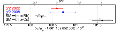
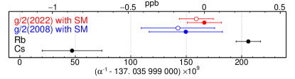
A new measurement, carried out blind of any measurement or prediction, determines to parts in (Fig. 1). Measured in a new apparatus in a lab at a different university, the new value is 2.2 times more precise than, and consistent with, the one that stood for 14 years [37]. In the most precise confrontation of theory and measurement, the SM prediction agrees to 1 part in . Our determination and the SM calculation are precise enough for a test that is 10 times more precise, once the discrepancy in measured values [40, 41] is resolved.
A one-electron quantum cyclotron is used. This is essentially a single electron suspended in a magnetic field and cooled to its lowest quantum states [42]. The magnetic moment operator for a spin-1/2 electron,
| (1) |
is proportional to its spin , normalized to its spin eigenvalue . The energy levels are
| (2) |
where . The cyclotron frequency is and . The spin frequency is and . In terms of these frequencies, and the anomaly frequency ,
| (3) |
An important feature of an electron measurement (not available with muons [43], for example) is that its cyclotron frequency can be measured in situ. The electron thus serves as its own magnetometer insofar as cancels out of the frequency ratios. Choosing to measure rather than (called making a measurement) significantly reduces the effect of frequency measurement uncertainties. However, it does not evade or reduce at all the largest measurement correction and its uncertainty, as we shall see.
A stable magnetic field is still critical at our precision because and are not measured simultaneously. Field drift of 2 ppb/day [44] (4 times below that in [37]) makes possible round-the-clock measurements, improved statistical precision, and better investigations of uncertainties. The apparatus in Fig. 2a achieves this by supporting a 50 mK trap on a 4.2 K self-shielding solenoid [45] using a mixing chamber flexibly hanging from the rest of a dilution refrigerator [46].
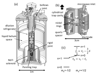
An electron in the field is trapped by adding an electrostatic quadrupole potential , with [47]. Cylindrical Penning trap electrodes [48, 49] (Fig. 2b) with appropriately chosen relative dimensions and potentials produce such a potential for a centered electron, which then oscillates nearly harmonically along at the axial frequency MHz. For T, the trap-modified cyclotron and anomaly frequencies are GHz and MHz [47]. A circular magnetron motion at kHz is cooled by axial sideband cooling [50, 47] and its effect is negligible during the measurement. Figure 2c shows the lowest cyclotron and spin energy levels and the frequency spacings, including a relativistic mass shift, , given by [47, 51].
The lowest cyclotron states for each spin are effectively stable because the spin is so nearly uncoupled from its environment [47]. Without a trap, the cyclotron state has a lifetime s. With a trap that is also a low-loss microwave cavity, this rate for the spontaneous emission of synchrotron radiation is inhibited by a factor of 50 to 70. Cyclotron excitations can then be detected before decay, when is chosen so is far from resonance with cavity radiation modes [52]. The cyclotron damping contributes 0.03 Hz to the cyclotron and anomaly linewidths (to be discussed), a negligible 0.2 ppt and a very important 0.2 ppb, respectively. Blackbody photons that excite to are eliminated by cooling the trap cavity below 100 mK [42].
The Brown-Gabrielse invariance theorem [53],
| (4) |
provides the and needed in Eq. (3) to determine . It is critical that Eq. (4) is invariant under unavoidable misalignments of B and the axis of , and under elliptic distortions of . The hierarchy allows an expansion of Eq. (4) that suffices for our precision to be inserted in Eq. (3), so
| (5) |
with and (defined in Fig. 2c) to be deduced with from measured line shapes. The added cavity-shift arises because the cyclotron frequency couples to radiation modes of the trap cavity, shifting both and [54, 55]. This measurement correction and its uncertainty are not reduced or evaded by a measurement. They must be determined and corrected at the full precision of .
To measure the needed in Eq. (5), the current induced in the electrodes by the axial oscillation is sent through a resonant circuit that is the input of a cryogenic HEMT amplifier. The 1-minute Fourier transform of the amplifier output in Fig. 3c illustrates the Johnson noise and electron signal canceling to make a dip that reveals [56]. Energy loss in the circuit damps the axial motion with a time constant ms. The amplifier heats the electron axial motion to K.
Small shifts in provide quantum nondemolition detection (QND) of one-quantum spin and cyclotron jumps, without the detection changing the cyclotron or spin state. Saturated nickel rings (Fig. 2b) produce a magnetic bottle gradient, with . This couples spin and cyclotron energies to , which then shifts by Hz. (The and are 5 and 3 times smaller than used previously [37].) To rapidly detect jumps after the cyclotron and anomaly drives are turned off, the amplified signal is immediately fed back to the electron. This self-excited oscillator (SEO) [57] resonantly and rapidly drives itself to a large amplitude even if shifts with amplitude, whereupon the gain is adjusted to maintain the amplitude. A Fourier transform of the large signal reveals the small that signals cyclotron and spin jumps.
Quantum jump spectroscopy produces anomaly and cyclotron resonances (Fig. 3a-b) from which to extract and to use in Eq. (5). Cyclotron and anomaly quantum jump trials are alternated. The magnetic field drift of 0.2 ppb/hr in the new apparatus is slow enough to correct using a quadratic fit to the lowest cyclotron drive frequencies that produce excitations. Each cyclotron and anomaly quantum jump trial starts with resonant anomaly and cyclotron drives that prepare the electron in the spin-up ground state, , followed by 1 s of axial magnetron sideband cooling [50, 47].
Cyclotron jumps to are driven by a 5 s microwave drive injected between trap electrodes (Fig. 2b), with an off-resonance anomaly drive also applied. Jumps occur in less than 20% of the trials to avoid saturation effects. Cavity-inhibited spontaneous emission [52] makes the excitation persist long enough so that self-excitation feedback [57] can be turned on in the next 1 s to detect the 1.3 Hz shift that signals a cyclotron quantum jump.
Anomaly quantum jumps are driven by an oscillatory potential applied to trap electrodes for 30 s to drive an off-resonance axial oscillation of the electron through the radial magnetic gradient . A cyclotron drive remains applied but is off resonance. The electron sees the oscillating magnetic field perpendicular to as needed to flip its spin, with a radial gradient that allows a simultaneous cyclotron transition [47]. A spontaneous decay to the spin-down ground state, , would be detected during the 60 s (more than 10 cyclotron decay times) after the drives are turned off. A maximum jump rate of 40% suggests a slight power broadening, but is still determined far more precisely than .
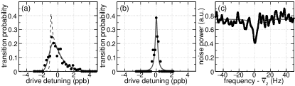
Well-understood, asymmetric cyclotron and symmetric anomaly line shapes are predicted [58] for thermal axial motion at temperature within a magnetic gradient . To this, the effect of cyclotron decay has been added [59]. The average oscillation amplitude squared is , where is the Boltzmann constant. The average field for the electron is shifted by and broadened by the same amount. The cyclotron bandwidth corresponds to a time ms needed to establish . This is much faster than the ms scale on which the axial amplitude fluctuates, so the predicted cyclotron line shape (dashed in Fig. 3a) approximates an exponential Boltzmann shape, centered at frequency . The anomaly transition time s is much slower than the axial amplitude fluctuations, whereupon the predicted thermal anomaly line is essentially symmetric about and is negligibly narrow. The observed anomaly linewidth of 0.06 Hz (0.35 ppb) in Fig. 3b is from other sources. Half is from the cyclotron decay lifetime and half is from applying the anomaly drive for only 30 s.
The anomaly line shape is consistent with what is predicted but the cyclotron line shape is not. Presumably this is due to unwanted magnetic field fluctuations that are averaged differently in the anomaly and cyclotron line shapes. Such fluctuations, with a 200 Hz bandwidth, were observed with a superconducting solenoid being jostled by its environment [60]. The anomaly line shape would average away such fluctuations to yield the narrow line observed (e.g. Fig. 3b). The cyclotron line shape would not, giving a possible explanation for the observed 0.5–0.8 ppb broadening (e.g. Fig. 3a).
Both and are extracted from such line shapes. Cyclotron line shapes are fit to the predicted line shape (dashed in Fig. 3a), convoluted with a Gaussian function to accommodate the broadening. Such a fit, illustrated by the solid curve in Fig. 3a, typically gives a 2 ppb cyclotron linewidth, a Gaussian broadening width of about 0.5 ppb, K, and with an uncertainty of about ppb. For anomaly line shapes (e.g. Fig. 3b), nearly symmetric and fractionally narrower by about a factor of 4, the uncertainty in is thus not very significant for the final uncertainty. Fitting with or without Gaussian broadening makes little difference (e.g. solid curve in Fig. 3b).
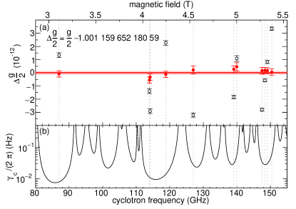
The cavity-shift in Eq. (5), the only correction to what is directly measured, arises because the cyclotron oscillator couples to radiation modes of the trap cavity and shifts [55, 54]. It is the downside of the cavity-inhibited spontaneous emission that desirably narrows resonance lines, and makes it possible to observe a cyclotron excitation before it decays. The cylindrical trap was invented [48] to allow cavity modes and shifts to be understood and calculated. Nonetheless, the mode frequencies and values must still be measured because of energy losses in induced surface currents, imperfect cavity machining, slits that make cavity sections into separately-biased trap electrodes, and dimension changes as the cavity cools below 100 mK from 300 K. Three consistent methods are used: (1) parametrically-pumped electrons [61, 62, 59], (2) measuring how long one electron stays in its first excited cyclotron state [37, 59], and (3) a new method of observing the decay time of an electron exited to .
A renormalized calculation [55, 54] with added cyclotron damping [37, 59] avoids the infinite cavity shifts that result from summing all mode contributions. This calculation assumes the mode frequencies of a perfect cylinder, one for TE modes, and another for TM modes. We calculate with dimensions chosen to best match observed frequencies and a single value for all modes. After shifts from the 72 observed modes using the ideal frequencies and the one value are subtracted out, contributions for these modes using measured frequencies and values are added back in. The leading contribution to cavity shift uncertainties comes from modifications of the field that an electron sees from imperfections and misalignments of the trap cavity. Figure 4a shows the consistency of determinations at 11 different magnetic fields, after each receives a different cavity shift.
A weighted average of the 11 determinations gives
| (6) |
with 1 uncertainty in the last two digits in parentheses. Figure 1 shows the good agreement of this 2022 determination at Northwestern with our 2008 determination at Harvard [37] and an uncertainty that is improved by a factor of 2.2. Because uncertainty correlations from similar measurement methods are difficult to determine, we do not recommend averaging our two determinations. Table 1 lists uncertainty contributions to the final result. The statistical uncertainty is from the fits that extract and . The two dominant uncertainties have been discussed – cyclotron broadening and cavity shifts (treated as correlated for nearby fields). The nuclear paramagnetism uncertainty is based upon the measured temperature fluctuations of the silver trap electrodes. The anomaly power shift uncertainty comes from the measured frequency dependence on drive strength.
| Source | Uncertainty |
|---|---|
| statistical | 0.29 |
| cyclotron broadening | 0.94 |
| cavity correction | 0.90 |
| nuclear paramagnetism | 0.12 |
| anomaly power shift | 0.10 |
| magnetic field drift | 0.09 |
| total | 1.3 |
Several SM sectors together predict
| (7) | |||||
The Dirac prediction [20] is first on the right. QED provides the asymptotic series in powers of , along with the muon and tauon contributions [38]. The constants [21], [22, 23], [24, 25] and [26] are calculated exactly, but require measured lepton mass ratios as input [29]. The measurements are so precise that a numerically calculated tenth order [28, 27] is required and tested. A second evaluation of [39] differs slightly for reasons not yet understood and the open points in Figs. 1 and 5 use this alternative. Hadronic and weak interaction contributions are [30, 31, 32] and [33, 34, 35, 36]. The exact and the numerical are remarkable advances that reduce the calculation uncertainty well below the uncertainties reported for the measured and .
The most precise measurements [40, 41], needed for the SM prediction of in Eq. (7), disagree by 5.5 , about ten times our measurement uncertainty (Fig. 1). Until the discrepancy is resolved, the best that can be said is that the predicted and measured agree to about , half of the discrepancy. A generic chiral symmetry model [63] then suggests that the electron radius is less than m, and that the mass of possible electron constituents must exceed GeV/. If would equal our determination uncertainty, then m and TeV/.
A 2.2 times reduced would bring us to the level of the intriguing standard deviation discrepancy between the measured and predicted muon magnetic moment [43, 64]. The muon’s BSM sensitivity, expected to be 40,000 times higher (the ratio of muon and electron masses), is largely offset by our 3150 times smaller uncertainty.
The fine structure constant is the fundamental measure of the strength of the electromagnetic interaction in the low energy limit. For the SI system of units, is a measure of the vacuum permittivity , given that and , and the speed of light are now defined [65]. Our and the SM give
| (8) | |||||
with theoretical and experimental uncertainties in the first and second brackets. Figure 5 compares to the measurements (black) that disagree with each other by 5.5 . Our value differs by 2.1 standard deviations from the Paris Rb determination of [41] and by 3.9 standard deviations from the Berkeley Cs determination [40]. The in [39] would change only “66” to “59” in Eq. (8).
For the future, a measurement is underway to realize the new precision with a positron, to improve the test of the fundamental symmetry invariance of the SM by a factor of 40 [66]. Much larger improvements in the precision of now seem feasible given the demonstration of more stable apparatus, improved statistics, and better understood uncertainties. Detectors being tested, more harmonic and lower loss trap cavities, and detector backaction circumvention methods [67, 68] should enable much more precise measurements to come.
In conclusion, an electron magnetic moment measurement is carried out blind to previous measurements and predictions. A PhD thesis [69] and a longer publication in preparation give fuller accounts. In new apparatus at a different university, the measured is consistent with our 2008 measurement, with a factor of 2.2 improved precision. The most precise prediction of the SM agrees with the most precise determination of a property of an elementary particle to about part in . When discrepant measurements are resolved, the new measurement uncertainty of parts in is available for a more precise test for BSM physics
Acknowledgements.
Early contributions were made by S. E. Fayer. NSF 2110565 provided the support, with X. Fan supported by the Masason Foundation. Detector development is supported by the Templeton Foundation, and low-loss trap cavity development is supported by the DOE SQMS Center.References
- [1] A. D. Sakharov, Soviet Journal of Experimental and Theoretical Physics Letters 5, 24 (1967).
- [2] G. Gamow, Phys. Rev. 70, 572 (1946).
- [3] F. Zwicky, Helvetica Physica Acta 6, 110 (1933).
- [4] V. C. Rubin, J. Ford, W. K., and N. Thonnard, Astrophys. J. 238, 471 (1980).
- [5] S. Perlmutter et al., The Astrophysical Journal 517, 565 (1999).
- [6] A. G. Riess et al., The Astronomical Journal 116, 1009 (1998).
- [7] A. Linde, Physics Letters B 108, 389 (1982).
- [8] A. Starobinsky, Physics Letters B 91, 99 (1980).
- [9] A. Starobinsky, Physics Letters B 117, 175 (1982).
- [10] A. H. Guth, Phys. Rev. D 23, 347 (1981).
- [11] P. Brax, A.-C. Davis, B. Elder, and L. K. Wong, Phys. Rev. D 97, 084050 (2018).
- [12] E. J. Chun, J. Kim, and T. Mondal, Journal of High Energy Physics 2019, 68 (2019).
- [13] G. F. Giudice, P. Paradisi, and M. Passera, Journal of High Energy Physics 2012, 113 (2012).
- [14] A. Aboubrahim, T. Ibrahim, and P. Nath, Phys. Rev. D 89, 093016 (2014).
- [15] M. Endo, K. Hamaguchi, and G. Mishima, Phys. Rev. D 86, 095029 (2012).
- [16] H. Davoudiasl and W. J. Marciano, Phys. Rev. D 98, 075011 (2018).
- [17] M. Bauer, M. Neubert, S. Renner, M. Schnubel, and A. Thamm, Phys. Rev. Lett. 124, 211803 (2020).
- [18] J. Liu, C. E. M. Wagner, and X.-P. Wang, Journal of High Energy Physics 2019, 8 (2019).
- [19] M. Endo and W. Yin, Journal of High Energy Physics 2019, 122 (2019).
- [20] P. A. M. Dirac, Proceedings of the Royal Society of London Series A 118, 351 (1928).
- [21] J. Schwinger, Phys. Rev. 73, 416 (1948).
- [22] A. Petermann, Helv. Phys. Acta 30, 407 (1957).
- [23] C. M. Sommerfield, Ann. Phys. (N.Y.) 5, 26 (1958).
- [24] T. Kinoshita, Phys. Rev. Lett. 75, 4728 (1995).
- [25] S. Laporta and E. Remiddi, Phys. Lett. B 379, 283 (1996).
- [26] S. Laporta, Physics Letters B 772, 232 (2017).
- [27] T. Aoyama, T. Kinoshita, and M. Nio, Phys. Rev. D 97, 036001 (2018).
- [28] T. Aoyama, M. Hayakawa, T. Kinoshita, and M. Nio, Phys. Rev. Lett. 109, 111807 (2012).
- [29] A. Kurz, T. Liu, P. Marquard, and M. Steinhauser, Nuclear Physics B 879, 1 (2014).
- [30] D. Nomura and T. Teubner, Nucl. Phys. B 867, 236 (2013).
- [31] A. Kurz, T. Liu, P. Marquard, and M. Steinhauser, Physics Letters B 734, 144 (2014).
- [32] Jegerlehner, Fred, EPJ Web Conf. 218, 01003 (2019).
- [33] K. Fujikawa, B. W. Lee, and A. I. Sanda, Phys. Rev. D 6, 2923 (1972).
- [34] A. Czarnecki, B. Krause, and W. J. Marciano, Phys. Rev. Lett. 76, 3267 (1996).
- [35] M. Knecht, M. Perrottet, E. de Rafael, and S. Peris, Journal of High Energy Physics 11, 003 (2002).
- [36] A. Czarnecki, W. J. Marciano, and A. Vainshtein, Phys. Rev. D 67, 073006 (2003).
- [37] D. Hanneke, S. Fogwell, and G. Gabrielse, Phys. Rev. Lett. 100, 120801 (2008).
- [38] T. Aoyama, T. Kinoshita, and M. Nio, Atoms 7, 28 (2019).
- [39] S. Volkov, Phys. Rev. D 100, 096004 (2019).
- [40] R. H. Parker, C. Yu, W. Zhong, B. Estey, and H. Müller, Science 360, 191 (2018).
- [41] L. Morel, Z. Yao, P. Cladé, and S. Guellati-Khélifa, Nature 588, 61 (2020).
- [42] S. Peil and G. Gabrielse, Phys. Rev. Lett. 83, 1287 (1999).
- [43] B. Abi et al., Phys. Rev. Lett. 126, 141801 (2021).
- [44] X. Fan, S. E. Fayer, and G. Gabrielse, Review of Scientific Instruments 90, 083107 (2019).
- [45] G. Gabrielse and J. Tan, J. Appl. Phys. 63, 5143 (1988).
- [46] G. Gabrielse, S. Fayer, T. Myers, and X. Fan, Atoms 7, 45 (2019).
- [47] L. S. Brown and G. Gabrielse, Rev. Mod. Phys. 58, 233 (1986).
- [48] G. Gabrielse and F. C. MacKintosh, Intl. J. of Mass Spec. and Ion Proc. 57, 1 (1984).
- [49] J. Tan and G. Gabrielse, Appl. Phys. Lett. 55, 2144 (1989).
- [50] R. S. Van Dyck, Jr., P. B. Schwinberg, and H. G. Dehmelt, in New Frontiers in High Energy Physics, edited by B. Kursunoglu, A. Perlmutter, and L.Scott (Plenum, New York, 1978), p. 159.
- [51] G. Gabrielse, H. Dehmelt, and W. Kells, Phys. Rev. Lett. 54, 537 (1985).
- [52] G. Gabrielse and H. Dehmelt, Phys. Rev. Lett. 55, 67 (1985).
- [53] L. S. Brown and G. Gabrielse, Phys. Rev. A 25, 2423 (1982).
- [54] L. S. Brown, G. Gabrielse, K. Helmerson, and J. Tan, Phys. Rev. Lett. 55, 44 (1985).
- [55] L. S. Brown, G. Gabrielse, K. Helmerson, and J. Tan, Phys. Rev. A 32, 3204 (1985).
- [56] D. J. Wineland and H. G. Dehmelt, J. Appl. Phys. 46, 919 (1975).
- [57] B. D’Urso, R. Van Handel, B. Odom, D. Hanneke, and G. Gabrielse, Phys. Rev. Lett. 94, 113002 (2005).
- [58] L. S. Brown, Ann. Phys. (N.Y.) 159, 62 (1985).
- [59] D. Hanneke, S. Fogwell Hoogerheide, and G. Gabrielse, Phys. Rev. A 83, 052122 (2011).
- [60] J. W. Britton, J. G. Bohnet, B. C. Sawyer, H. Uys, M. J. Biercuk, and J. J. Bollinger, Phys. Rev. A 93, 062511 (2016).
- [61] J. Tan and G. Gabrielse, Phys. Rev. A 48, 3105 (1993).
- [62] J. Tan and G. Gabrielse, Phys. Rev. Lett. 67, 3090 (1991).
- [63] S. J. Brodsky and S. D. Drell, Phys. Rev. D 22, 2236 (1980).
- [64] T. Aoyama et al., Physics Reports 887, 1 (2020).
- [65] M. Stock, R. Davis, E. de Mirandés, and M. J. T. Milton, Metrologia 56, 022001 (2019).
- [66] S. Fogwell Hoogerheide, J. C. Dorr, E. Novitski, and G. Gabrielse, Review of Scientific Instruments 86, 053301 (2015).
- [67] X. Fan and G. Gabrielse, Phys. Rev. Lett. 126, 070402 (2021).
- [68] X. Fan and G. Gabrielse, Phys. Rev. A 103, 022824 (2021).
- [69] X. Fan, Ph.D. thesis, Harvard University, 2022, (thesis advisor: G. Gabrielse).