Measurement of the photosphere oblateness of Cassiopeiae via Stellar Intensity Interferometry with the VERITAS Observatory
Abstract
We use the stellar intensity interferometry system implemented with the Very Energetic Radiation Imaging Telescope Array System (VERITAS) at Fred Lawrence Whipple Observatory (FLWO) as a light collector to obtain measurements of the rapid rotator star Cassiopeiae, at a wavelength of . Using data from baselines sampling different position angles, we extract the size, oblateness, and projected orientation of the photosphere. Fitting the data with a uniform ellipse model yields a minor-axis angular diameter of mas, a major-to-minor-radius ratio of , and a position angle of for the axis of rotation. A rapidly-rotating stellar atmosphere model that includes limb and gravity darkening describes the data well with a fitted angular diameter of mas corresponding to an equatorial radius of 10.9, a rotational velocity with a lower limit at that of breakup velocity, and a position angle of degrees. These parameters are consistent with H line spectroscopy and infrared-wavelength Michelson interferometric measurements of the star’s decretion disk. This is the first measurement of an oblate photosphere using intensity interferometry.
show]josieg.rose.86@gmail.com
1 Introduction
Spectroscopic measurements of the H line of the subgiant Cassiopeiae ( Cas) indicate that it is a Be-type star rotating at nearly its breakup velocity about an axis inclined by to our line of sight. Thus, it is expected to have a pronounced equatorial bulge. The history of Michelson interferometric measurements of Cas spans many decades (see §3 of Stee, Ph. et al., 2012, for a brief overview). These measurements reveal an extended decretion disk that suggests a position angle of the rotational axis, measured east of celestial north (Sigut et al., 2020). However, these measurements, performed at infrared wavelengths, are unable to measure the photosphere itself.
Stellar intensity interferometry (SII) at optical wavelengths has the potential to measure the photosphere itself at sub-milliarcsecond scale. Originally developed in the 1950’s and used through the early 1970’s (Hanbury Brown & Twiss, 1954; Hanbury Brown, 1974), SII has very recently seen a renaissance with the availability of large light collectors in imaging atmospheric Cherenkov telescope (IACT) arrays, high-speed electronics and modern computing at several observatories (Abeysekara et al., 2020; Abe et al., 2024; Zmija et al., 2023; Acharyya et al., 2024). By correlating the intensity of light at separated telescopes, rather than the wave amplitude (as done with Michelson interferometry), SII is robust against effects of optical imperfections, including atmospheric turbulence, and works well at optical wavelengths, providing sub-milliarcsecond resolutions with 100 m baselines. Relative to Michelson interferometry, this comes at a cost of reduced signal-to-noise for the same observing duration.
In this paper, we present the first SII measurement sensitive to the shape, as well as the size, of a star. The work is organized as follows. Section 2 gives a brief description of the VERITAS stellar intensity interferometer (VSII) and the datasets discussed here. Section 3 presents the data analysis and extracted squared visibilities. Section 4 uses simple geometric models of the star to extract size, shape, and orientation information from the measurements. The dependence of the squared visibility on and is fitted with uniform disk and uniform ellipse models. Section 5 discusses a complete stellar model of a rapid rotator with limb and gravitational darkening. Comparison of our data with this model provides tight constraints on the size, rotational speed, and orientation of the star. In Section 6, we summarize and provide an outlook for future work.
2 Instrument and Dataset
VERITAS is composed of four 12-m diameter IACTs, usually used for very high-energy () gamma-ray astronomy (Holder et al., 2006). During bright-moon periods, the system is used for SII measurements. The four telescopes are individually referred to as T1, T2, T3, and T4, and are unequally spaced with separations ranging between about 80 and 170 meters, and interferometric projected baselines ranging between about 35 and 170 meters. We have presented further details of the VSII stellar intensity interferometer in previous publications (Abeysekara et al., 2020; Acharyya et al., 2024). The optical light from the observed star is detected by a single Hamamatsu super-bialkali R10560 photomultiplier tube (PMT) located at the telescope focal plane, and continuously digitized at a 250 MHz rate with 8 bit resolution. We use a narrow-band filter () with a bandpass of 10 nm to focus on the photosphere of the star. An upgrade associated with the present study is the use of a CPU-based server that simultaneously correlates all six telescope pairs with a frequency-domain algorithm. This correlator produces correlations identical to the FPGA-based correlator using a time-based algorithm that was used in our previous measurements (Scott, 2023). For some observations in the present paper, a 10-MHz clock improved the start-time synchronization.
| UTC Date | Telescope Pairs Used | Observation Time | Target - Moon Angle |
|---|---|---|---|
| (yyyy-mm-dd) | (,) | (hours) | (degrees) |
| 2023-01-08 | (1,3), (2,3), (2,4), (3,4) | 4.5 | 79 |
| 2023-02-02 | (1,2), (1,3), (2,3), (2,4), (3,4) | 3.25 | 62 |
| 2023-12-25 | (2,4) | 2.0 | 51 |
| 2023-12-26 | (1,2), (1,3), (2,3), (2,4), (3,4) | 7.28 | 56 |
| 2023-12-27 | (1,2), (1,3), (2,3), (2,4), (3,4) | 6.0 | 63 |
| 2024-02-19 | (1,2), (1,3), (1,4), (2,3), (2,4), (3,4) | 2.5 | 59 |
| 2024-02-20 | (1,2), (1,3), (2,3), (2,4) | 2.0 | 66 |
| 2024-02-21 | (1,3), 2,3) | 1.0 | 74 |
| 2024-02-22 | (1,3), (2,3), (2,4), (3,4) | 1.75 | 82 |
| 2024-05-18 | (1,2), (2,3), (3,4) | 1.0 | MBH |
| 2024-05-19 | (1,2), (2,3), (3,4) | 1.0 | MBH |
| 2024-12-13 | (1,2), (1,3), (2,3), (2,4), (3,4) | 2.0 | 46 |
| 2024-12-15 | (1,2), (1,3), (2,3), (3,4) | 1.0 | 55 |
| 2024-12-17 | (1,3), (2,3), (2,4), (3,4) | 1.0 | 70 |
Note. — MBH denotes moon below horizon.
Dates and durations of VSII observations of Cas are listed, together with the Moon angle and the telescope pairs used. The four VERITAS telescopes are identified by numbers from one to four. The Moon angle is the angle between the Moon and the observed star. It correlates with the night sky background level affecting the data. Only a subset of telescope pairs from each observation were used in the analysis because some telescopes were not working, they had too large of a baseline, or the data was too noisy.
Table 1 lists the Cas observations for which data were collected, over 6 bright moon periods between January 2023 and December 2024. Intensity interferometry is generally robust against ambient light for bright stars; VSII operations are reliable for target-to-moon angles from to (Kieda et al., 2021). Target-to-moon angles are listed in table 1.
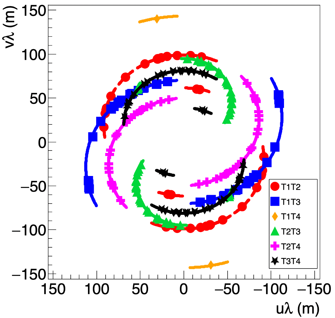
Over 160 pair-hours of data were used, after quality cuts discussed below. The baseline coverage in the star image Fourier reciprocal () plane is shown in figure 1. The relative telescope separation lies in the plane, the celestial east-north plane, following general interferometric convention. (See § 4 of Thompson et al. (2001) and Dravins et al. (2013) for a further description of the plane.)
3 Data Analysis
3.1 Overview
The size and shape of the photosphere are determined by measuring the dependence of the intensity correlation on the length and orientation of the projected baseline (i.e. separation between the telescopes perpendicular to the direction of the starlight) and then fitting this data to a model. In this section, we discuss the steps taken to measure the intensity correlation between pairs of telescopes; they are similar to those we have presented previously (Abeysekara et al., 2020; Acharyya et al., 2024).
The relative-time intensity correlation is measured as a function of time during a run as described in section 3.2. After removing effects of night-sky background light (section 3.3) radio interference, and tracking corrections (section 3.4), the magnitude of the correlation is quantified by a Gaussian fit to the intensity correlation projected over a run, as discussed in section 3.5. Finally, in section 3.6 we identify some runs for which the noise is too large to find a correlation peak.
3.2 The correlogram
The current from the photomultiplier tube in each telescope is digitized and recorded at 250 MHz, i.e. in 4-ns samples. A correlogram is formed by convoluting the digitized waveforms from two telescopes and and normalizing by the product of the average values of the currents:
| (1) |
where indicates an average over time and is the relative time (“time lag”) between samples. The superscript (∗) denotes the correlation before correcting for effects of stray light, as discussed in section 3.3. The constant is set equal to the optical path delay between the telescopes at the beginning of the observation run. The normalized correlation is constructed every 2 seconds of time-in-run . We refer to these two-second intervals as “frames” below.
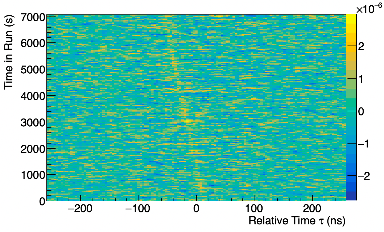
A correlogram for a 2-hour observation run with telescopes T2 and T4 is shown in figure 2. A clear correlation signal is visible close to at the beginning of the run, due to proper adjustment of (which we shall drop from further discussion for simplicity) in the correlator. The position of the correlation in relative time changes over the course of the run, as the star moves across the sky, which changes the optical path delay between the fixed telescope-pair positions.
3.3 Correction for residual light from other sources
During observation runs, the current in the phototubes is dominated by the light from the star. Some of the light incident on the phototubes does not come from the star of interest, but rather from the night sky background. This uncorrelated contribution leads to a reduction in the raw measured correlation signal (Rou et al., 2013). Neglecting this contribution would generate a run-by-run variation in the proportionality constant between the measured integral of the Gaussian fit of the correlation peaks and the actual squared visibility.
We correct for this effect as we have done previously (Abeysekara et al., 2020; Acharyya et al., 2024). Immediately before and after every observation run, the telescopes are pointed north of the star and the average currents are recorded. Depending on viewing conditions, stellar position, and moon angle and phase for a given observation run, the off-star current is of the on-star current.
The corrected correlogram is related to the raw correlogram (equation 1) as
| (2) |
where represents time-averaged stray-light current at time-in-run . We assume that during the observations on the star itself, the ambient contribution varies linearly with time between what we measure before and after the on-star run. Neglecting the stray light contamination would lead to a inaccuracy on the angular diameter estimate.
3.4 Removal of artifacts from tracking corrections and radio-frequency contamination
Some of the frames of the correlogram must be discarded before further processing, due to two effects.
The first comes from telescope tracking corrections. Occasionally (typically once an hour), the image of the star moves slightly off of the face of the photomultiplier tube. When this happens, the operator slightly adjusts the tracking parameters. During this procedure, the telescope briefly stops tracking altogether, and the current drops sharply, as starlight is no longer being registered. An example is seen in figure 3.
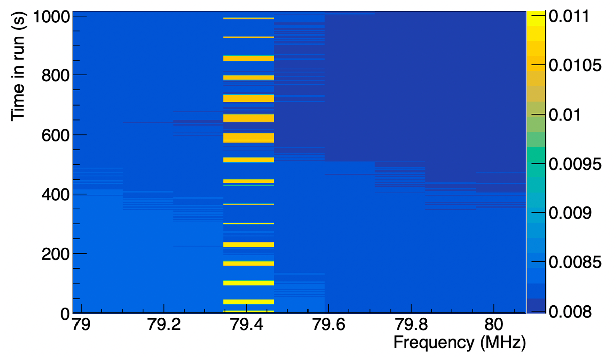
The second problem arises from an on-site radio repeater at FLWO, which transmits a 50 W signal at about 171 MHz in short ( sec), sporadic (roughly every 10-30 seconds) bursts. This results in a strong aliased sinusoidal correlation– more than 50 times larger than the physical correlation of interest– in all telescope pairs (Scott, 2023). In addition to producing the correlogram, the correlator server calculates the frequency power spectrum of each telescope for each frame, and the 79.4 MHz spikes are easily identified, as demonstrated in figure 4. Roughly one third of the frames are contaminated by this signal and are removed from the correlogram. Starting in late December, 2024, we received permission to disable the repeater during VSII running, resulting in cleaner data and effectively about 40% greater data collection efficiency.
Finally, for many runs and telescopes, there are much smaller frequency spikes at 93.7, 99.6, and 107.5 MHz present in every frame. The presence and strength of these signals depends on telescope orientation and vary from night to night. They are likely due to local radio stations. When observed, the resulting sinusoidal correlations are subtracted from the correlogram, frame-by-frame, as discussed in Acharyya et al. (2024).
3.5 Obtaining squared visibilities and their uncertainties
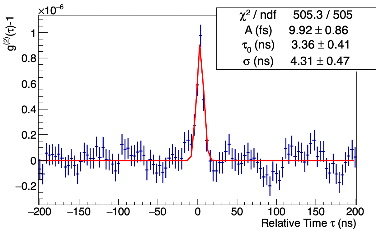
Once the bad frames are removed and radio-station signals subtracted, a one-dimensional correlation function as a function of relative time is produced by shifting each frame by the appropriate optical path delay () and averaging over frames, according to
| (3) |
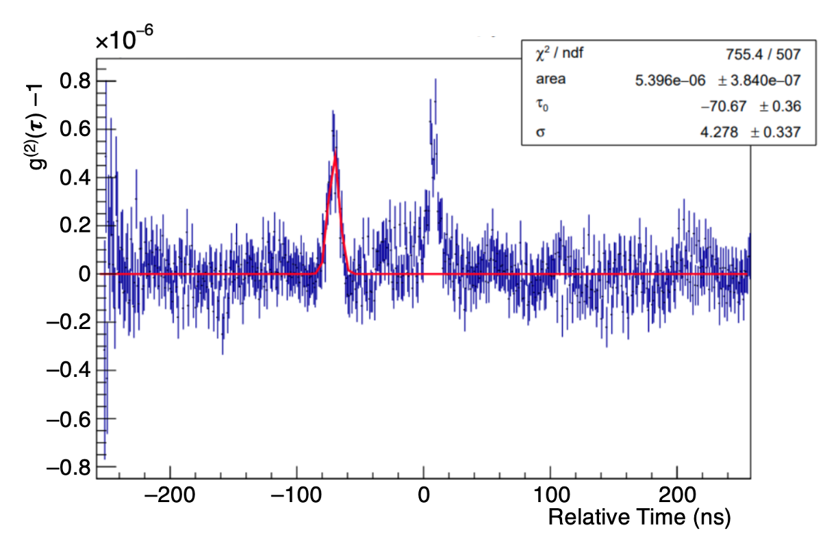
An example is shown in figure 5. A clear signal is observed close to relative time . Due to uncertainties on the clock cycle and exact start time, the peak position may vary on order 10 ns, from one run to another (Acharyya et al., 2024).
A Gaussian fit is performed on within a window ns. An actual correlation signal is expected to have a width around , due to the finite sampling and response time of the photomultiplier tube and preamp. If the peak-finder fails to find a peak in the window, or if its Gaussian width is less than 2 ns or greater than 6 ns, then the data is discarded. Variation of the window between ns and ns has a negligibly small effect on the measurements. The peak width cut was varied between 1.5 and 7 ns, and the effect of these variations is included in the systematic uncertainty estimate below. The integral of the Gaussian, measured in units of time and denoted in Figure 5, is proportional to the squared visibility (Acharyya et al., 2024). The proportionality constant, determined by the bandwidth of the optical filter, electronic response, and telescope optics, is expected (Matthews, 2020) to be on order ns. We treat this normalization constant as a parameter in our fits below.
The statistical uncertainty of this integral could be derived from the fit parameters, but this ignores the residual correlations present in the background. To arrive at a better estimate of the uncertainty that accounts for the residual background, we randomly add false peaks, with the same area as the fitted peak, on top of the background far from the signal region ( ns). We then perform the same Gaussian fitting and selection procedure on these false peaks as we do for the true peak. The standard deviation of the distribution of false-peak Gaussian integrals is taken as the uncertainty of the fitted peak near . The uncertainty extracted in this way is typically about 40% larger than what would be obtained if we ignored the residual correlated background. This procedure is illustrated in more detail in Appendix A.
We have reanalyzed the data of our previous measurement (Acharyya et al., 2024) of the slow rotator UMa, using our improved method of uncertainty estimations and removing tracking corrections. The resulting angular diameter for a uniform-disk fit changes by only 1% (well within stated uncertainties), but the /ndf is reduced from 2.30 to 1.04.
3.6 Exclusion of sub-threshold peaks
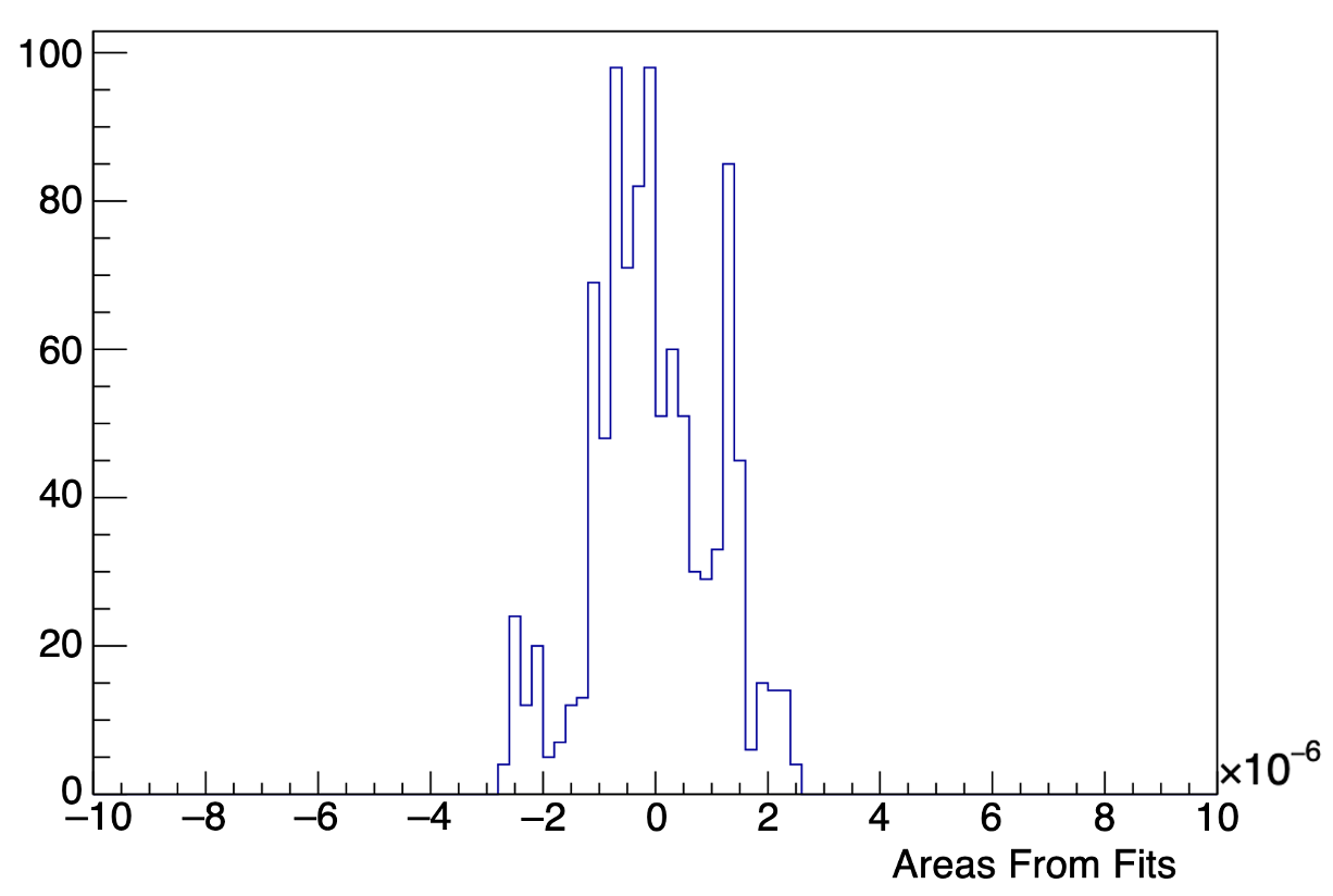
In the presence of statistical and residual correlated noise, any peak-finding algorithm finds spurious peaks when the actual signal is too small. To identify the threshold at which this occurs, we used the peak-finder in random regions on the background far from the actual peak region ( ns), again applying the same Gaussian fitting and selection criteria as for the actual signal peaks.
The resulting distribution of Gaussian integrals is shown in figure 6. As we have discussed previously (Acharyya et al., 2024), this results in a bimodal distribution with a strong dip at zero. We take twice the standard deviation of this distribution as a threshold, which includes 95% of the fits (Rose, 2025). Fitted peaks with integrals less than this threshold are indistinguishable from noise and are discarded when extracting the size and shape of the star, as discussed in sections 4 and 5.
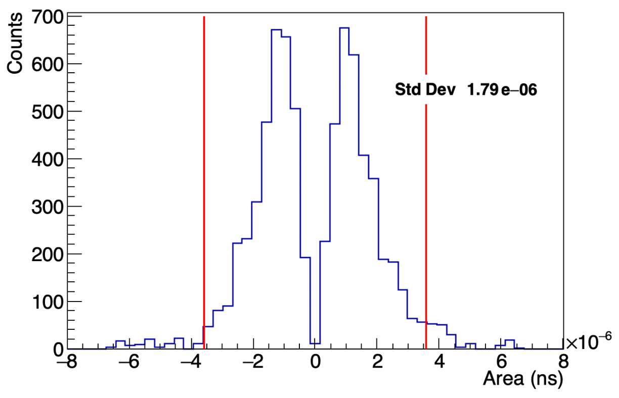
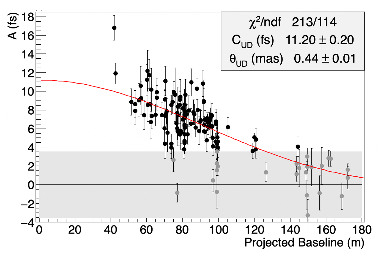
Figure 7 shows our measured visibilities as a function of the projected baseline. The gray points represent those that pass the peak selections discussed in section 3.5 but which fall below the noise threshold, shown as a gray band in the figure. These come from runs in which the noise is too large, or the signal too small, to distinguish actual signal peaks from the noise. These gray points are not used in further analysis. We have varied the threshold between 3.0 and 4.1 fs to obtain a systematic uncertainty on fit parameters discussed in section 4.
4 Extracting the size and shape of the photosphere
In this section, we fit the visibilities with simple models, to extract an effective size, shape, and orientation of the star. It is common to model a star as a uniformly illuminated disk of angular radius . In this case, the squared visibility for a projected baseline is
| (4) |
where nm and is the first-order Bessel function. is the proportionality constant between actual squared visibilities and peak integrals measured from correlation functions, which we treat as a fit parameter. The red curve in figure 7 is the best fit of equation 4 to the data. The effective uniform disk angular radius is mas, consistent with the result reported by the MAGIC collaboration (Abe et al., 2024) of . Our systematic uncertainties were calculated by varying the peak quality cuts and threshold and not removing tracking corrections or accounting for the background light contributions. As discussed below, this star is not expected to be circular, so some tension between the values of measured by different observatories may be expected.
A rapid rotator like Cas is expected have an equatorial bulge and anisotropic gravitational darkening, which would lead to an oblate source with spatial extension perpendicular to the axis of rotation. Therefore, fitting the data with a uniform circular disk may not be appropriate, as the length scale may depend on the orientation of the baseline. An intuitive way to explore this possibility is to measure the uniform disk effective angular size as a function of angle of the projected baseline in the plane, . The angle with the smallest effective angular diameter would correspond to the position angle of the star rotation axis.
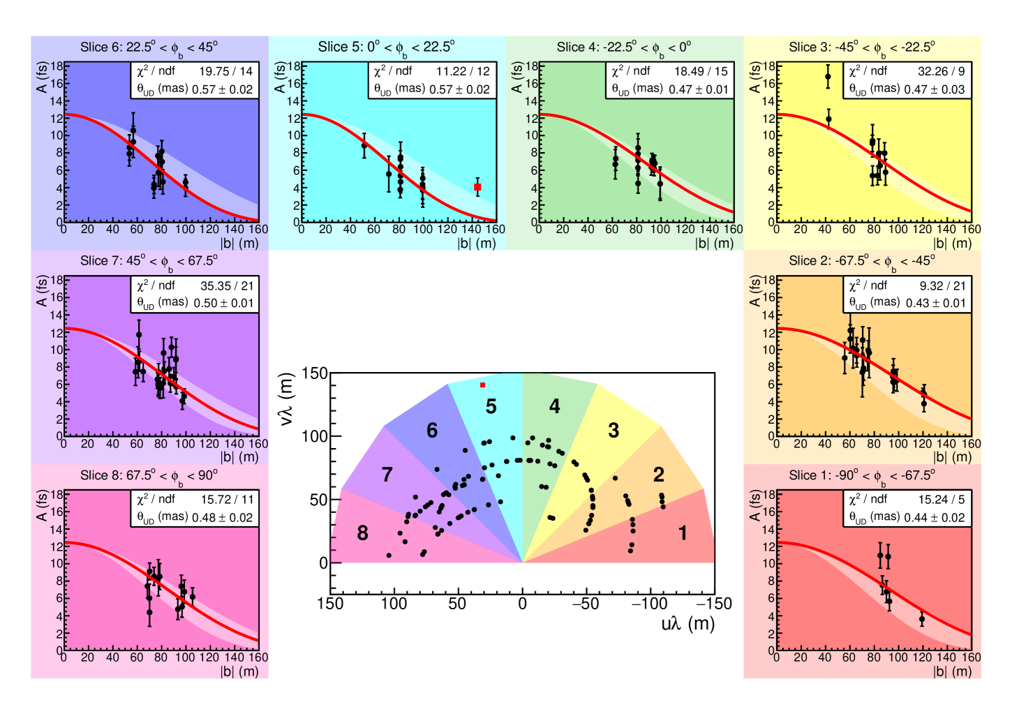
In figure 8, the visibility measurements are sorted according to ranges in . In the center panel, the baseline for each measurement is shown in the plane, and -wide slices are defined and shown as differently colored regions. Measurements that fall within each slice are shown in the surrounding panels and fitted with the uniform disk model of equation 4 to extract an effective one-dimensional angular diameter for a small range in . While the visibility measurement from T1T4 with baseline of 145 m passes our threshold cut (see figures 7 and 10), we suspect it may be a fluctuation, like those discussed in section 3.6. Therefore, we report fit parameters obtained both including and excluding this point, and it is drawn as a red square in Figures 8, 10, and 11.
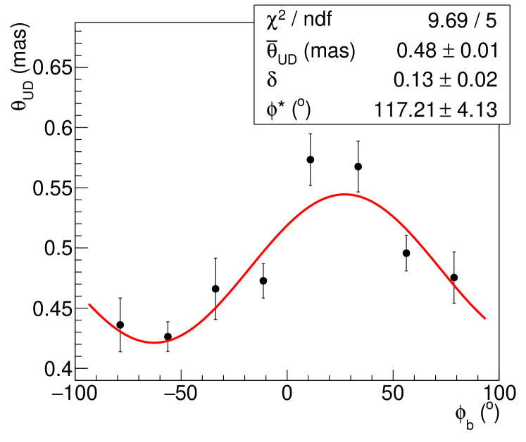
Figure 9 shows the effective angular diameter versus the average position angle of the slice. The data are well fit with the function
| (5) |
The average effective diameter is mas. The minimum diameter, the minor axis, is at , which we associate with the position angle of the stellar rotation axis and is consistent with previous measurements of the accretion disk of this star (Sigut et al., 2020). The extracted magnitude of the modulation, corresponds111If an oscillation is uniformly integrated over bins of width , the resulting histogram will exhibit oscillations of magnitude . In our case, this is small effect: the finite-binning-corrected oscillation magnitude is . to a maximum-to-minimum ratio of .
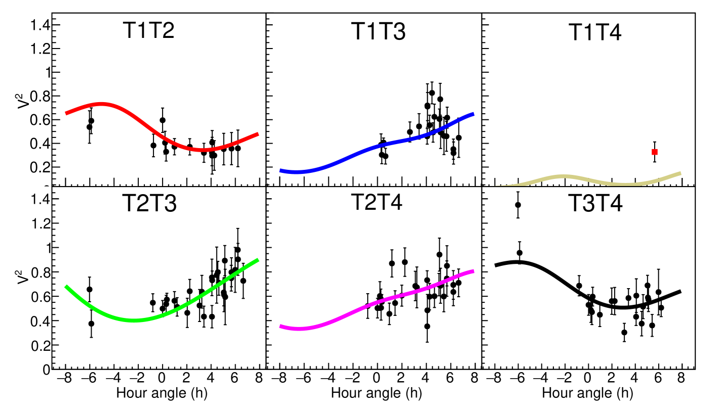
While figures 8 and 9 provide an intuitive way to estimate the anisotropy and orientation of the rapid rotator, it is more accurate to perform a simultaneous fit of all visibilities as a function of and . The hour angle, , for a given source and observatory, uniquely defines the coordinates for each telescope pair, so we fit the data as a function of hour angle (Dravins et al., 2013). The data is fitted with a uniformly illuminated ellipse model (Tycner et al., 2006)
| (6) |
where
| (7) |
Here, is the ratio of the major to minor axes (), is angular diameter of the minor axis, and is the position angle of the minor axis of the ellipse.222Note that Tycner et al. (2006) describes the model for . For a rapid rotator, then, is the position angle of the axis of rotation.
The proportionality between the actual squared visibility and the peak integrals is , which we treat as a fit parameter. Figure 10 shows the peak integrals (divided by ) for each telescope pair, as a function of local hour angle.
This more complete model describes the data better than the uniform disk model discussed above; see table 2. The angular size of the minor axis is mas, and the axis ratio is . Fitting an elliptical source with a uniform circular model (equation 4) would result in a uniform disk radius () somewhere between 0.43 mas and 0.55 mas, depending on the orientation of the baseline. Therefore, the value of extracted from any given measurement will depend on the orientation of the baselines used during observation. This complicates comparisons between, say VSII and MAGIC (Abe et al., 2024), when using a circular source model on a rapid rotator.
It also means that from equation 5 and from equation 4 represent slightly different quantities. While figures 8 and 9 are an intuitive way to display the non-circular nature of the star, the characteristics of the elliptical appearance of the star are most accurately extracted by a fit to an elliptical image model.
The extracted position angle of the rapid rotator star axis is estimated to be , consistent with measurements of the decretion disk at longer wavelengths (Sigut et al., 2020), indicating that the decretion disc is generally aligned along the equatorial bulge of the photosphere itself.
| T1T4 point | Model | (º) | (mas) | (fs) | ||
|---|---|---|---|---|---|---|
| Uniform Disk | - | 0.44 0.01 0.03 | (1) | 11.2 0.2 0.5 | 213/114 | |
| Excluded | uv slices | 117 4 6 | 0.42 0.02 0.02 | 1.30 0.05 0.03 | 12.4* | 9.69/5 |
| Uniform Ellipse | 116 5 7 | 0.43 0.02 0.02 | 1.28 0.04 0.02 | 12.4 0.5 0.5 | 170/112 | |
| Uniform Disk | - | 0.43 0.01 0.02 | (1) | 11.0 0.2 0.5 | 215/115 | |
| Included | uv slices | 118 4 6 | 0.41 0.01 0.02 | 1.27 0.05 0.04 | 12.2* | 7.39/5 |
| Uniform Ellipse | 117 5 8 | 0.42 0.02 0.02 | 1.27 0.05 0.03 | 12.2 0.5 0.5 | 178/113 |
Note. — note that for the uv slices analysis is based on sinusoidal fit to round model fits of the 8 “pizza slice” sections.
* for the uv slice model is fixed to from the Uniform Ellipse model fit.
Errorbars are reported as .
5 Constraining a stellar model of a rapid rotator
We have computed synthetic squared visibilities, high-resolution spectra and spectral energy distributions for the photosphere of Cas using PHOENIX (Hauschildt & Baron, 1999, version 20.01.02B), a code for nova, supernova, stellar and planetary model atmospheres. We use a Roche–von Zeipel model for a rapidly rotating star (Aufdenberg et al., 2006; Sackrider & Aufdenberg, 2023), modeled as an infinitely concentrated central mass under uniform angular rotation.
Each axially symmetric model is parameterized by a trigonometric parallax, , equatorial angular diameter, , polar effective temperature, , polar gravity, , fraction of the critical (breakup) angular rotation rate, , and the von Zeipel gravity darkening parameter, . As seen from Earth, the model is further parameterized by the inclination , and the position angle, , of the visible stellar rotation axis.
The intensity of each point on the surface of the model star, as viewed from Earth, is interpolated from a grid of 106 PHOENIX stellar atmosphere radiation fields: specific intensities at 78 direction cosines between surface normal and the direction of an observer and 106 () pairs (with step sizes of 500 K in and 0.1 in ) between the hot, high gravity pole and the cooler, lower gravity equator. A model rotating very close to the critical limit ( = 0.9999) has a surface temperature difference of 12000 K and a gravity difference of .
For our model of Cas we fixed mas (van Leeuwen, 2007, mas), as constrained by Lailey & Sigut (2024) (see also Sigut et al. (2020) and Tycner et al. (2006)), and , as empirically determined for rapid rotating stars imaged with CHARA/MIRC (Che et al., 2011).
We computed 7750 models for Cas with 31 values from 0.40 mas to 0.70 mas, 25 values from 90∘ to 138∘ and 10 values from 0.9000 to 0.9999. With six baselines and 118 hour angles, this corresponds to a table of 5,487,000 synthetic visibility values.
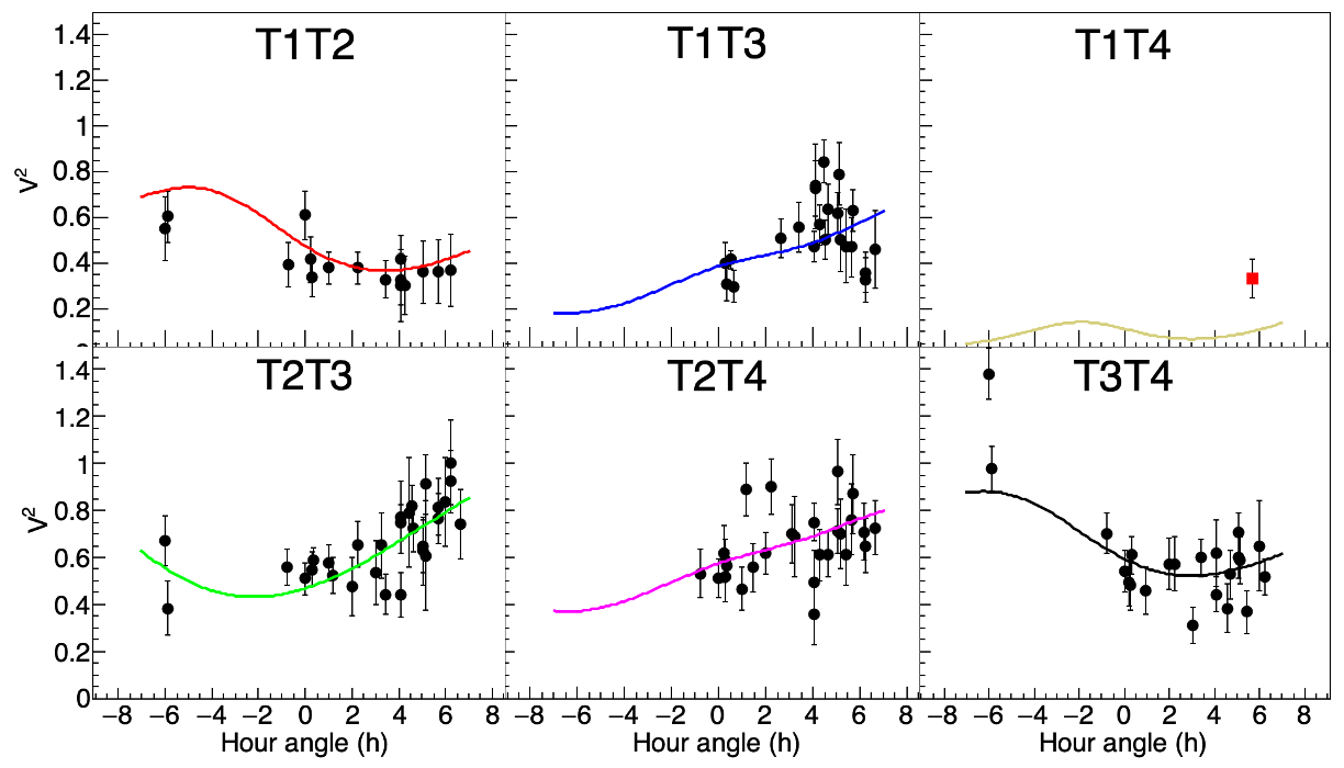
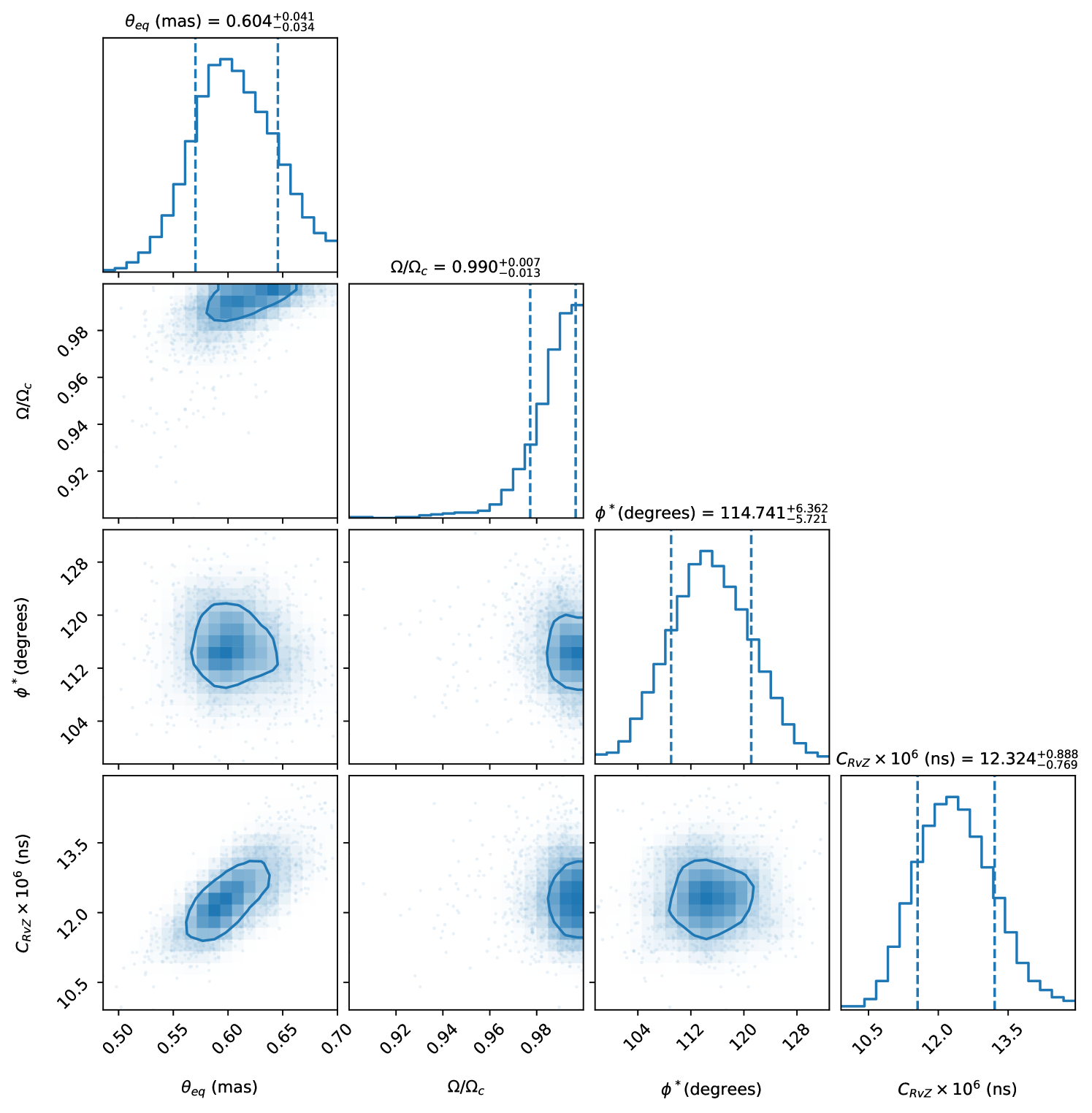
Figure 11 shows the VERITAS data (the same as in Figure 10) with a Roche-von Zeipel stellar model. Figure 12 shows the distributions of the best-fit parameters. The fit to the data confronts the upper physical bound of unity, therefore we can only define a lower limit on the rotation rate at 97.7%
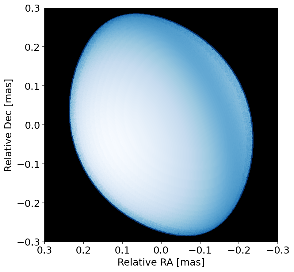
Figure 13 is a rendering of the calculated light intensity distribution corresponding to the Roche-von Zeipel model that fits the data best.
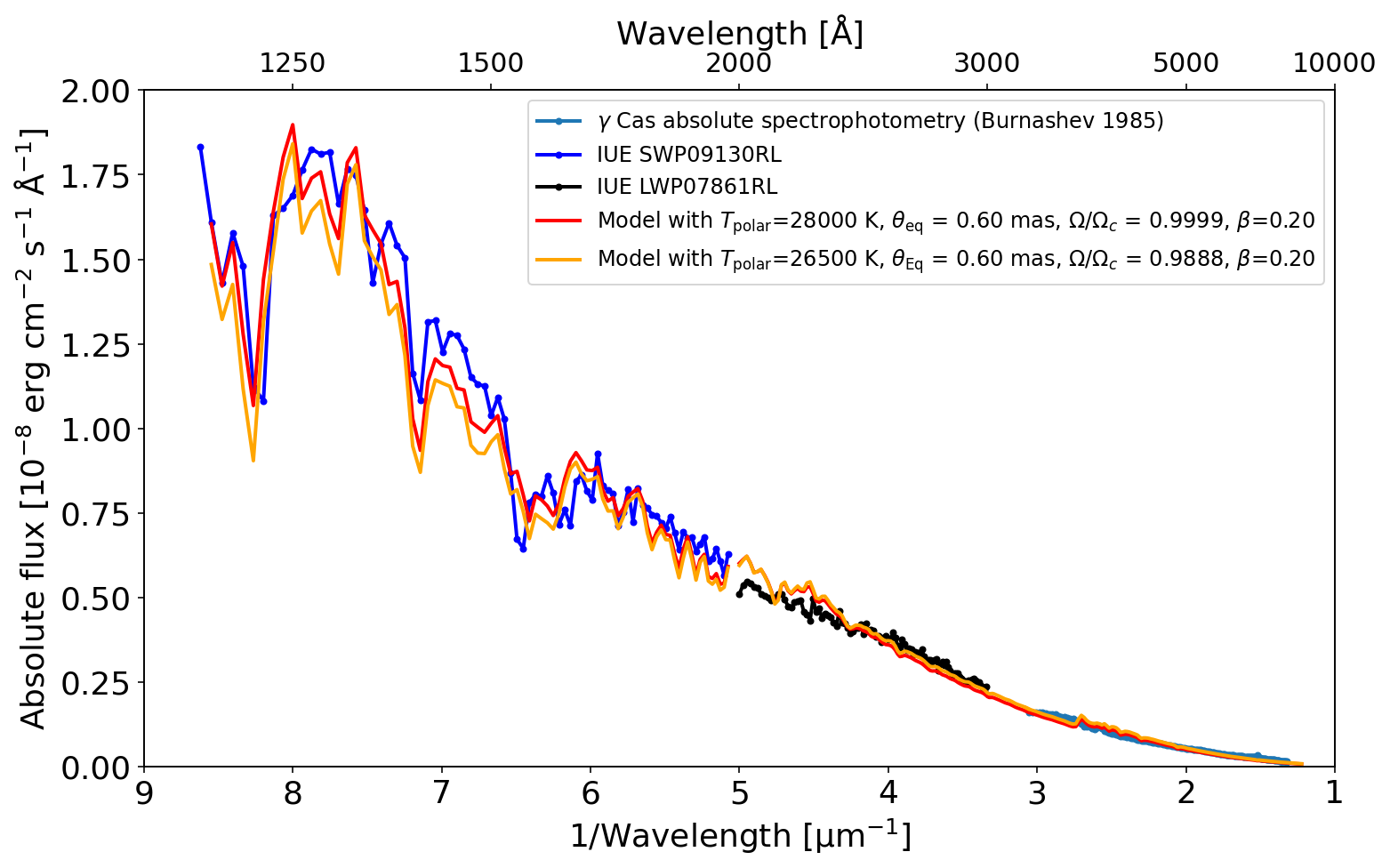
For the best-fitting median values, = 0.60 mas and = 0.99, = 26500 K provides a reasonable match to available absolute archival spectrophotometry in the UV optical range (see Figure 14). A = 3.82 yields a mass of 15.1 M⊙, at the top of the range 13-15 M⊙ adopted by Smith (2019). Table 3 shows the best fit and the derived parameters.
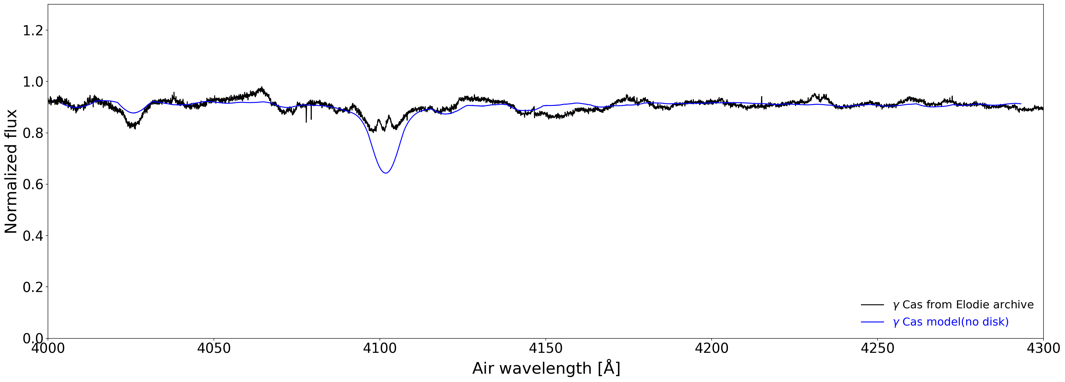
Our adopted polar gravity and inclination yield a projected rotation velocity of . Chauville et al. (2001) found values 420-425 by comparing models to the He I 4471 line. Figure 15 shows a comparison between the best-fit model to the squared visibility data and a high-resolution spectrum in the VSII band around 416 nm. Although the H line is filled with emission from the disk, the model roughly matches the wings of the line profile. The other recognizable absorption line is He I 4026, which is stronger than the model with roughly the same width.
| Parameter | Value | Reference |
|---|---|---|
| With a fixed inclination of the rotation axis, and gravity darkening = 0.2 | ||
| Equatorial angular diameter, (mas) | 0.605 | This paper |
| Fraction of critical rotation rate, | 0.990 | This paper |
| Parallax, (mas) | 5.940.12 | van Leeuwen (2007) |
| Equatorial radius, () | 10.9 | derived, |
| Polar Radius, () | 7.9 | derived, |
| With a fixed = 3.82, , gravity darkening = 0.2 | ||
| Mass, () | 152 | |
| Equatorial velocity, (km s-1), | 45020 | |
| Projected equatorial velocity, () | 389 20 | derived from and , see Figure 15 |
| Polar effective temperature, (K) | 26500 -28000 | spectrophotometry, see Figure 14 |
| Pole-equator difference, (K) | 9200 -12000 | derived, |
Note. — The parameters and depend on , while the equatorial velocity, , depends on
6 Summary and Outlook
We have used the VERITAS telescope array to perform intensity interferometry measurements on the rapid rotator Cassiopeiae, combining data from more than 160 pair-hours of observation. While the size and elongation of the decretion disk of this star have been well measured at infrared wavelengths, measurements of the photosphere at visible wavelengths have previously only been sensitive to its size. The six telescope pairs of the VSII observatory provide good coverage of the Fourier plane. By varying the orientation as well as the magnitude of the baseline between telescopes, we were able to measure the size, the equatorial bulge, and the orientation of the axis of rotation of the photosphere. This is the first time that intensity interferometry has been used to measure the oblateness of a star.
A uniform ellipse fit of our data indicates that the angular size of the minor axis of the photosphere is mas, with a major-to-minor axis ratio of . The position angle of the minor axis, which corresponds to the rotator axis, is , in agreement with earlier measurements of the accretion disk.
We have also compared our data to a Roche-von Zeipel model of a rapid rotator, which includes effects of limb and gravitational darkening as well as temperature gradients. The temperature profile was adjusted to match published spectrophotometry measurements. Our data is well fit within this model with an equatorial diameter of mas, position angle of degrees, and a lower limit on the angular velocity very near the critical value, . The equatorial radius is 10.9 and the mass of the star in the model is .
Previous stellar intensity interferometry measurements have been limited to extracting the overall size of the photosphere and resolving the extended decretion disk in its H light (Matthews et al., 2023). In order to take advantage of our coverage in the plane and gain sensitivity to the stellar shape, we found it important to remove artifacts from external radio interference and manual tracking corrections. Our remaining systematic uncertainties are dominated by uncertainties in the clock start synchronization, the peak-finding algorithm, and by residual correlated noise in the background. The overall systematic error is on the order of the statistical error, suggesting that only adding hours at previously unobserved hour angles would increase the precision of our measurement.
Having established the capability of stellar intensity interferometry to measure not only the size, but also the shape and orientation of a photosphere, we are continuing analysis of other rapid rotators, to expand the scope of data in the stellar catalog of bright stars. This will provide valuable input and constraints to stellar models that must match both the spectral and the geometrical consequences of extreme rotation.
Acknowledgments
This research is supported by grants from the U.S. Department of Energy Office of Science, the U.S. National Science Foundation and the Smithsonian Institution, by NSERC in Canada, and by the Helmholtz Association in Germany. We acknowledge the excellent work of the technical support staff at the Fred Lawrence Whipple Observatory and the collaborating institutions in the construction and operation of the VERITAS and VSII instruments. The authors gratefully acknowledge support under NSF grants #AST 1806262, #PHY 2117641, and #PHY 2111531 for the construction and operation of the VSII instrumentation. We acknowledge the support of the Ohio Supercomputer Center and of an Ohio State University College of Arts and Sciences Exploration Grant. We acknowledge the financial support of the French National Research Agency (project I2C, ANR-20-CE31-0003). This work made use of the High Performance Cluster “Vega” at Embry-Riddle Aeronautical University. This research has made use of the VizieR catalogue access tool, CDS, Strasbourg, France (DOI : 10.26093/cds/vizier). The original description of the VizieR service was published in 2000, A&AS 143, 23. Part of this research is based on INES data from the IUE satellite.
Appendix A Calculating uncertainties on peak areas with correlated background contribution
This appendix illustrates in more detail the calculation of an uncertainty on the area of the Gaussian peak, which we discuss in section 3.5. Figure 16 shows an example of a fit to a simulated peak located at about -70 ns in relative time, with the same area as the original correlation peak located at 0 ns in relative time. The simulated peak is inserted into the background noise away from the peak, fitted with the same procedure as the original peak, and subjected to the same quality cuts. This is repeated about 5000 times for each correlation function. The differences between the areas found from these fits and the true area of the simulated peak are added to a distribution like the one shown in figure 17. The uncertainty on the peak area is the RMS of this distribution, which describes how much the background noise can distort the area.
Appendix B Unnormalized visibilities above threshold
| UTC Date (yyyy-mm-dd hh:mm) | Pair | Area (fs) | Baseline (m) | u (m) | v (m) | Hour angle (h) |
|---|---|---|---|---|---|---|
| 2023-12-25 01:57 | T2T4 | 7.2 1.0 | 95.5 | -82.5 | 47.6 | 0.28 |
| 2023-12-25 03:04 | T2T4 | 6.8 1.3 | 90.0 | -86.2 | 25.0 | 1.44 |
| 2023-12-26 01:34 | T1T2 | 7.4 1.3 | 96.2 | -90.4 | -32.4 | 0.00 |
| 2023-12-26 01:34 | T1T2 | 4.6 0.9 | 98.5 | -83.5 | -51.9 | 0.98 |
| 2023-12-26 01:34 | T1T3 | 5.1 0.5 | 120.0 | -108.9 | 48.2 | 0.50 |
| 2023-12-26 01:34 | T2T3 | 6.2 0.8 | 94.3 | -15.5 | 92.9 | 0.00 |
| 2023-12-26 01:34 | T2T3 | 7.0 0.9 | 92.5 | -28.4 | 88.0 | 0.98 |
| 2023-12-26 01:34 | T2T4 | 6.3 1.0 | 96.5 | -80.5 | 52.8 | 0.00 |
| 2023-12-26 01:34 | T2T4 | 5.7 1.1 | 92.5 | -85.7 | 34.3 | 0.97 |
| 2023-12-26 01:34 | T3T4 | 6.6 1.1 | 76.5 | -65.0 | -40.1 | 0.01 |
| 2023-12-26 01:34 | T3T4 | 5.6 1.2 | 78.8 | -57.5 | -53.7 | 0.97 |
| 2023-12-26 03:37 | T2T3 | 5.8 1.5 | 89.2 | -40.1 | 79.6 | 2.04 |
| 2023-12-26 03:37 | T2T3 | 6.5 1.6 | 84.7 | -48.5 | 69.3 | 3.05 |
| 2023-12-26 03:37 | T2T4 | 7.5 1.1 | 86.6 | -85.3 | 14.3 | 1.99 |
| 2023-12-26 03:37 | T2T4 | 8.5 1.5 | 78.4 | -78.0 | -6.6 | 3.10 |
| 2023-12-26 03:37 | T3T4 | 7.0 1.3 | 80.2 | -45.7 | -65.8 | 1.99 |
| 2023-12-26 03:37 | T3T4 | 3.8 0.9 | 80.9 | -29.7 | -75.1 | 3.06 |
| 2023-12-26 05:38 | T1T2 | 4.0 1.4 | 99.4 | -30.3 | -94.4 | 4.07 |
| 2023-12-26 05:38 | T1T2 | 4.4 1.7 | 99.2 | -7.5 | -98.6 | 5.04 |
| 2023-12-26 05:38 | T1T3 | 5.7 0.8 | 92.0 | -83.9 | -37.1 | 4.07 |
|---|---|---|---|---|---|---|
| 2023-12-26 05:38 | T2T3 | 5.4 1.1 | 78.6 | -53.6 | 57.3 | 4.07 |
| 2023-12-26 05:38 | T2T3 | 7.9 1.4 | 71.2 | -54.9 | 45.2 | 5.04 |
| 2023-12-26 05:38 | T2T4 | 9.1 1.0 | 70.1 | -66.2 | -22.6 | 4.07 |
| 2023-12-26 05:38 | T2T4 | 8.7 1.1 | 61.7 | -50.2 | -35.5 | 5.03 |
| 2023-12-26 05:38 | T3T4 | 5.4 0.9 | 81.1 | -12.6 | -80.0 | 4.07 |
| 2023-12-26 05:38 | T3T4 | 8.6 1.0 | 81.1 | 4.9 | -80.8 | 5.04 |
| 2023-12-26 07:39 | T1T2 | 4.5 1.9 | 99.3 | 20.3 | -96.7 | 6.21 |
| 2023-12-26 07:39 | T1T3 | 4.4 1.1 | 73.8 | -31.3 | -65.8 | 6.21 |
| 2023-12-26 07:39 | T2T3 | 12.2 2.2 | 60.3 | -51.7 | 31.0 | 6.20 |
| 2023-12-26 07:39 | T2T4 | 8.6 1.5 | 53.6 | -26.6 | -45.7 | 6.21 |
| 2023-12-26 07:39 | T3T4 | 6.3 0.9 | 81.0 | 25.1 | -76.6 | 6.21 |
| 2023-12-27 01:43 | T1T2 | 5.0 1.2 | 96.8 | -89.4 | -36.5 | 0.20 |
| 2023-12-27 01:43 | T1T3 | 3.6 0.8 | 119.2 | -109.8 | 44.2 | 0.66 |
| 2023-12-27 01:43 | T2T3 | 6.4 0.9 | 91.9 | -31.0 | 86.5 | 1.20 |
| 2023-12-27 01:43 | T2T4 | 7.5 1.5 | 95.8 | -82.0 | 49.1 | 0.20 |
| 2023-12-27 01:43 | T2T4 | 10.8 1.4 | 91.4 | -86.1 | 30.1 | 1.18 |
| 2023-12-27 01:43 | T3T4 | 6.0 1.2 | 77.1 | -63.8 | -43.1 | 0.21 |
| 2023-12-27 03:44 | T1T2 | 4.6 0.9 | 99.7 | -66.7 | -73.7 | 2.24 |
| 2023-12-27 03:44 | T1T3 | 6.2 1.1 | 105.4 | -104.3 | -5.8 | 2.65 |
| 2023-12-27 03:44 | T2T3 | 8.0 1.2 | 88.5 | -42.0 | 77.7 | 2.24 |
| 2023-12-27 03:44 | T2T3 | 7.9 1.7 | 83.7 | -49.7 | 67.2 | 3.24 |
| 2023-12-27 03:44 | T2T4 | 11.0 1.5 | 84.9 | -84.2 | 9.4 | 2.24 |
| 2023-12-27 03:44 | T2T4 | 8.4 2.1 | 77.3 | -76.6 | -8.8 | 3.22 |
| 2023-12-27 03:44 | T3T4 | 7.0 1.4 | 80.4 | -42.2 | -68.3 | 2.24 |
| 2023-12-27 05:47 | T1T2 | 3.7 1.6 | 99.3 | -25.8 | -95.6 | 4.26 |
| 2023-12-27 05:47 | T1T3 | 6.9 1.0 | 90.0 | -79.9 | -40.7 | 4.27 |
| 2023-12-27 05:47 | T1T3 | 9.6 1.7 | 81.6 | -60.2 | -54.8 | 5.14 |
| 2023-12-27 05:47 | T2T3 | 11.1 1.5 | 70.5 | -54.9 | 44.1 | 5.13 |
|---|---|---|---|---|---|---|
| 2023-12-27 05:47 | T2T4 | 7.4 1.3 | 68.4 | -63.2 | -25.5 | 4.27 |
| 2023-12-27 05:47 | T2T4 | 8.5 1.8 | 60.7 | -47.9 | -37.0 | 5.16 |
| 2023-12-27 05:47 | T3T4 | 7.1 1.2 | 81.1 | 6.3 | -80.8 | 5.12 |
| 2023-01-08 05:23 | T1T3 | 7.8 1.3 | 86.1 | -71.5 | -47.5 | 4.66 |
| 2023-01-08 05:23 | T1T3 | 7.7 1.1 | 76.9 | -45.4 | -61.6 | 5.70 |
| 2023-01-08 05:23 | T2T3 | 8.8 1.3 | 74.4 | -54.8 | 50.3 | 4.64 |
| 2023-01-08 05:23 | T2T3 | 9.3 1.3 | 65.7 | -53.9 | 37.5 | 5.66 |
| 2023-01-08 05:23 | T2T4 | 7.5 1.2 | 64.9 | -56.7 | -31.0 | 4.67 |
| 2023-01-08 05:23 | T2T4 | 9.3 1.8 | 56.7 | -37.7 | -42.0 | 5.68 |
| 2023-01-08 05:23 | T3T4 | 6.4 1.2 | 81.1 | -1.9 | -81.0 | 4.66 |
| 2023-02-02 03:10 | T1T2 | 5.1 1.3 | 99.4 | -29.8 | -94.6 | 4.09 |
| 2023-02-02 03:10 | T1T3 | 8.8 1.5 | 91.7 | -83.4 | -37.6 | 4.10 |
| 2023-02-02 03:10 | T1T3 | 7.5 1.1 | 82.2 | -61.7 | -53.8 | 5.07 |
| 2023-02-02 03:10 | T2T3 | 9.1 0.9 | 78.4 | -53.7 | 57.1 | 4.09 |
| 2023-02-02 03:10 | T2T3 | 7.6 1.7 | 71.0 | -54.9 | 44.9 | 5.07 |
| 2023-02-02 03:10 | T2T4 | 6.0 1.6 | 70.0 | -65.9 | -22.9 | 4.08 |
| 2023-02-02 03:10 | T2T4 | 11.7 1.7 | 61.4 | -49.4 | -36.0 | 5.07 |
| 2023-02-02 03:10 | T3T4 | 7.5 1.7 | 81.1 | -12.3 | -80.0 | 4.08 |
| 2023-02-02 03:10 | T3T4 | 7.3 1.1 | 81.1 | 5.5 | -80.8 | 5.08 |
| 2023-02-02 05:12 | T1T3 | 4.0 1.2 | 73.6 | -31.0 | -66.0 | 6.22 |
| 2023-02-02 05:12 | T2T3 | 11.2 1.6 | 60.2 | -51.7 | 30.8 | 6.22 |
| 2023-02-02 05:12 | T2T4 | 7.9 1.4 | 53.5 | -26.5 | -45.8 | 6.21 |
| 2024-02-19 02:31 | T1T3 | 6.1 1.0 | 87.2 | -73.9 | -45.7 | 4.55 |
| 2024-02-19 02:31 | T2T3 | 9.9 1.1 | 75.1 | -54.7 | 51.3 | 4.55 |
| 2024-02-19 02:31 | T3T4 | 4.7 1.3 | 81.1 | -4.1 | -80.9 | 4.54 |
| 2024-02-19 03:38 | T1T2 | 4.4 1.7 | 99.2 | 7.9 | -98.6 | 5.68 |
| 2024-02-19 03:38 | T1T3 | 5.7 1.6 | 77.4 | -46.9 | -61.0 | 5.65 |
| 2024-02-19 03:38 | T1T4 | 4.1 1.1 | 144.4 | -31.1 | -140.4 | 5.65 |
|---|---|---|---|---|---|---|
| 2024-02-19 03:38 | T2T3 | 9.9 1.5 | 65.5 | -53.8 | 37.3 | 5.68 |
| 2024-02-19 03:38 | T2T4 | 10.6 2.1 | 56.7 | -37.5 | -42.1 | 5.68 |
| 2024-02-20 02:07 | T1T2 | 3.7 1.9 | 99.4 | -29.9 | -94.6 | 4.09 |
| 2024-02-20 02:07 | T1T3 | 9.0 2.3 | 91.8 | -83.6 | -37.5 | 4.09 |
| 2024-02-20 02:07 | T2T3 | 9.4 1.9 | 78.6 | -53.7 | 57.4 | 4.07 |
| 2024-02-20 02:07 | T2T4 | 4.4 1.6 | 70.1 | -66.1 | -22.7 | 4.07 |
| 2024-02-20 03:14 | T1T3 | 6.1 1.7 | 81.3 | -59.4 | -55.3 | 5.17 |
| 2024-02-20 03:14 | T2T3 | 7.4 2.8 | 70.2 | -54.9 | 43.7 | 5.16 |
| 2024-02-21 02:22 | T1T3 | 10.3 1.1 | 88.1 | -75.8 | -44.2 | 4.46 |
| 2024-02-21 02:22 | T2T3 | 9.6 2.9 | 75.8 | -54.6 | 52.5 | 4.46 |
| 2024-02-22 03:26 | T1T3 | 5.8 2.0 | 78.9 | -52.4 | -58.9 | 5.44 |
| 2024-02-22 03:26 | T2T4 | 7.4 1.6 | 58.5 | -42.7 | -39.9 | 5.43 |
| 2024-02-22 03:26 | T3T4 | 4.5 1.1 | 81.1 | 11.9 | -80.2 | 5.44 |
| 2024-02-22 03:59 | T2T3 | 10.2 2.3 | 62.7 | -52.9 | 33.5 | 5.98 |
| 2024-02-22 03:59 | T3T4 | 7.9 2.3 | 81.0 | 21.4 | -78.1 | 5.98 |
| 2024-02-22 04:32 | T1T3 | 5.6 2.1 | 71.5 | -18.8 | -68.7 | 6.65 |
| 2024-02-22 04:32 | T2T3 | 9.0 1.8 | 55.7 | -49.4 | 25.7 | 6.65 |
| 2024-02-22 04:32 | T2T4 | 8.8 1.4 | 51.4 | -17.2 | -48.2 | 6.64 |
| 2024-05-18 10:00 | T1T2 | 6.7 1.7 | 62.4 | -14.9 | 60.2 | -6.02 |
| 2024-05-18 10:00 | T2T3 | 8.2 1.3 | 80.1 | 52.8 | 60.1 | -6.02 |
| 2024-05-18 10:00 | T3T4 | 16.8 1.3 | 42.0 | -21.4 | 35.8 | -6.02 |
| 2024-05-19 10:07 | T1T2 | 7.3 1.4 | 62.8 | -18.4 | 59.6 | -5.87 |
| 2024-05-19 10:07 | T2T3 | 4.7 1.4 | 81.0 | 52.2 | 61.9 | -5.87 |
| 2024-05-19 10:07 | T3T4 | 11.9 1.1 | 42.6 | -23.7 | 35.1 | -5.88 |
| 2024-12-13 01:34 | T1T2 | 4.8 1.2 | 93.3 | -91.6 | -16.6 | -0.75 |
| 2024-12-13 01:34 | T2T3 | 6.8 0.9 | 94.9 | -4.1 | 94.7 | -0.80 |
| 2024-12-13 01:34 | T2T4 | 6.5 1.3 | 98.6 | -72.3 | 66.8 | -0.80 |
| 2024-12-13 01:34 | T3T4 | 8.5 1.0 | 73.7 | -68.1 | -27.8 | -0.80 |
| 2024-12-13 02:40 | T1T2 | 4.1 1.0 | 97.0 | -88.9 | -38.3 | 0.29 |
|---|---|---|---|---|---|---|
| 2024-12-13 02:40 | T1T3 | 4.8 1.1 | 121.1 | -108.4 | 53.4 | 0.29 |
| 2024-12-13 02:40 | T2T3 | 6.7 0.9 | 93.8 | -19.5 | 91.7 | 0.30 |
| 2024-12-13 02:40 | T2T4 | 6.3 1.3 | 95.4 | -82.6 | 47.4 | 0.29 |
| 2024-12-13 02:40 | T3T4 | 5.8 1.3 | 77.3 | -63.2 | -44.4 | 0.29 |
| 2024-12-15 05:43 | T1T2 | 4.0 1.0 | 99.6 | -44.7 | -88.7 | 3.41 |
| 2024-12-15 05:43 | T1T3 | 6.8 1.3 | 98.6 | -95.6 | -23.4 | 3.40 |
| 2024-12-15 05:43 | T2T3 | 5.4 1.1 | 82.7 | -50.8 | 65.2 | 3.41 |
| 2024-12-15 05:43 | T3T4 | 7.3 1.0 | 81.0 | -23.8 | -77.2 | 3.41 |
| 2024-12-17 02:28 | T1T3 | 3.8 0.9 | 120.8 | -108.8 | 51.9 | 0.35 |
| 2024-12-17 02:28 | T2T3 | 7.1 0.6 | 93.7 | -20.3 | 91.4 | 0.36 |
| 2024-12-17 02:28 | T2T4 | 6.9 0.7 | 95.2 | -83.0 | 46.2 | 0.36 |
| 2024-12-17 02:28 | T3T4 | 7.4 1.0 | 77.5 | -62.7 | -45.2 | 0.36 |
References
- Abe et al. (2024) Abe, S., Abhir, J., Acciari, V. A., et al. 2024, Monthly Notices of the Royal Astronomical Society, 529, 4387, doi: 10.1093/mnras/stae697
- Abeysekara et al. (2020) Abeysekara, A. U., Benbow, W., Brill, A., et al. 2020, Nature Astronomy, 4, 1164–1169, doi: 10.1038/s41550-020-1143-y
- Acharyya et al. (2024) Acharyya, A., et al. 2024, Astrophys. J., 966, 28, doi: 10.3847/1538-4357/ad2b68
- Astropy Collaboration et al. (2018) Astropy Collaboration, Price-Whelan, A. M., Sipőcz, B. M., et al. 2018, AJ, 156, 123, doi: 10.3847/1538-3881/aabc4f
- Aufdenberg et al. (2006) Aufdenberg, J. P., Mérand, A., Coudé du Foresto, V., et al. 2006, ApJ, 645, 664, doi: 10.1086/504149
- Brun & Rademakers (1997) Brun, R., & Rademakers, F. 1997, Nucl. Instrum. Meth. A, 389, 81, doi: 10.1016/S0168-9002(97)00048-X
- Chauville et al. (2001) Chauville, J., Zorec, J., Ballereau, D., et al. 2001, A&A, 378, 861, doi: 10.1051/0004-6361:20011202
- Che et al. (2011) Che, X., Monnier, J. D., Zhao, M., et al. 2011, ApJ, 732, 68, doi: 10.1088/0004-637X/732/2/68
- Dravins et al. (2013) Dravins, D., LeBohec, S., Jensen, H., & Nuñez, P. D. 2013, Astroparticle Physics, 43, 331, doi: https://doi.org/10.1016/j.astropartphys.2012.04.017
- Earl et al. (2022) Earl, N., Tollerud, E., Jones, C., et al. 2022, astropy/specutils: V1.7.0, v1.7.0, Zenodo, doi: 10.5281/zenodo.6207491
- Foreman-Mackey (2016) Foreman-Mackey, D. 2016, The Journal of Open Source Software, 1, 24, doi: 10.21105/joss.00024
- González-Riestra et al. (2000) González-Riestra, R., Cassatella, A., Solano, E., Altamore, A., & Wamsteker, W. 2000, A&AS, 141, 343, doi: 10.1051/aas:2000317
- Hanbury Brown (1974) Hanbury Brown, R. 1974, The intensity interferometer. Its applications to astronomy (London: Taylor & Francis Ltd.)
- Hanbury Brown & Twiss (1954) Hanbury Brown, R., & Twiss, R. 1954, The London, Edinburgh, and Dublin Philosophical Magazine and Journal of Science, 45, 663, doi: 10.1080/14786440708520475
- Hauschildt & Baron (1999) Hauschildt, P. H., & Baron, E. 1999, Journal of Computational and Applied Mathematics, 109, 41, doi: 10.48550/arXiv.astro-ph/9808182
- Holder et al. (2006) Holder, J., Atkins, R., Badran, H., et al. 2006, Astroparticle Physics, 25, 391, doi: https://doi.org/10.1016/j.astropartphys.2006.04.002
- James & Roos (1975) James, F., & Roos, M. 1975, Comput. Phys. Commun., 10, 343, doi: 10.1016/0010-4655(75)90039-9
- Kieda et al. (2021) Kieda, D., et al. 2021, PoS, ICRC2021, 803, doi: 10.22323/1.395.0803
- Lailey & Sigut (2024) Lailey, B. D., & Sigut, T. A. A. 2024, MNRAS, 527, 2585, doi: 10.1093/mnras/stad3321
- Matthews (2020) Matthews, N. 2020, PhD thesis, University of Utah
- Matthews et al. (2023) Matthews, N., Rivet, J.-P., Vernet, D., et al. 2023, AJ, 165, 117, doi: 10.3847/1538-3881/acb142
- Moultaka et al. (2004) Moultaka, J., Ilovaisky, S. A., Prugniel, P., & Soubiran, C. 2004, PASP, 116, 693, doi: 10.1086/422177
- Rose (2025) Rose, J. 2025, Bachelor’s honors thesis, The Ohio State University. https://kb.osu.edu/handle/1811/105962
- Rou et al. (2013) Rou, J., Nuñez, P. D., Kieda, D., & LeBohec, S. 2013, Monthly Notices of the Royal Astronomical Society, 430, 3187, doi: 10.1093/mnras/stt123
- Sackrider & Aufdenberg (2023) Sackrider, J. L., & Aufdenberg, J. P. 2023, Research Notes of the American Astronomical Society, 7, 216, doi: 10.3847/2515-5172/ad023b
- Scott (2023) Scott, M. 2023, Bachelor’s honors thesis, The Ohio State University. http://hdl.handle.net/1811/102963
- Sigut et al. (2020) Sigut, T. A. A., Mahjour, A. K., & Tycner, C. 2020, ApJ, 894, 18, doi: 10.3847/1538-4357/ab8386
- Smith (2019) Smith, M. A. 2019, PASP, 131, 044201, doi: 10.1088/1538-3873/aaf70b
- Stee, Ph. et al. (2012) Stee, Ph., Delaa, O., Monnier, J. D., et al. 2012, A&A, 545, A59, doi: 10.1051/0004-6361/201219234
- Thompson et al. (2001) Thompson, A. R., Moran, J. M., & Swenson Jr., G. W. 2001, Interferometry and Synthesis in Radio Astronomy (WILEY‐VCH Verlag GmbH & Co. KGaA)
- Torrado & Lewis (2021) Torrado, J., & Lewis, A. 2021, J. Cosmology Astropart. Phys, 2021, 057, doi: 10.1088/1475-7516/2021/05/057
- Tycner et al. (2006) Tycner, C., Gilbreath, G. C., Zavala, R. T., et al. 2006, Astron. J., 131, 2710, doi: 10.1086/502679
- van Leeuwen (2007) van Leeuwen, F. 2007, A&A, 474, 653, doi: 10.1051/0004-6361:20078357
- Virtanen et al. (2020) Virtanen, P., Gommers, R., Oliphant, T. E., et al. 2020, Nature Methods, 17, 261, doi: 10.1038/s41592-019-0686-2
- Zmija et al. (2023) Zmija, A., Vogel, N., Wohlleben, F., et al. 2023, Monthly Notices of the Royal Astronomical Society, 527, 12243, doi: 10.1093/mnras/stad3676