Measurements of the Intensity and Polarization of the Anomalous Microwave Emission in the Perseus molecular complex with QUIJOTE
Abstract
Anomalous microwave emission (AME) has been observed in numerous sky regions, using different experiments in the frequency range GHz. One of the most scrutinized regions is G159.6-18.5, located within the Perseus molecular complex. In this paper we present further observations of this region (194 hours in total over deg2), both in intensity and in polarization. They span four independent frequency channels between 10 and 20 GHz, and were gathered with QUIJOTE, a new CMB experiment with the goal of measuring the polarization of the CMB and Galactic foregrounds. When combined with other publicly-available intensity data, we achieve the most precise spectrum of the AME measured to date in an individual region, with 13 independent data points between 10 and 50 GHz being dominated by this emission. The four QUIJOTE data points provide the first independent confirmation of the downturn of the AME spectrum at low frequencies, initially unveiled by the COSMOSOMAS experiment in this region. We accomplish an accurate fit of these data using models based on electric dipole emission from spinning dust grains, and also fit some of the parameters on which these models depend.
We also present polarization maps with an angular resolution of and a sensitivity of K/beam. From these maps, which are consistent with zero polarization, we obtain upper limits of and ( C.L.) respectively at 12 and 18 GHz, a frequency range where no AME polarization observations have been reported to date. These constraints are compatible with theoretical predictions of the polarization fraction from electric dipole emission originating from spinning dust grains. At the same time, they rule out several models based on magnetic dipole emission from dust grains ordered in a single magnetic domain, which typically predict higher polarization levels. Future QUIJOTE data in this region may allow more stringent constraints on the polarization level of the AME.
keywords:
cosmology: cosmic microwave background - radiation mechanisms: general - ISM: individual objects: G159.6-18.5 - diffuse radiation - radio continuum: ISM.1 Introduction
Now that the observations of the temperature anisotropies of the Cosmic Microwave Background (CMB) have reached levels of sensitivity and angular resolution that have allowed the determination of the main cosmological parameters with accuracies close to (Bennett et al., 2013; Planck Collaboration et al., 2014c), attention has shifted to the study of the polarization of these anisotropies. CMB polarization also encodes a wealth of cosmological information. In particular, it is of paramount importance to study the B-mode anisotropy, which can only be created by vector or tensor perturbations, such as those due to primordial gravitational waves (Kamionkowski et al., 1997; Zaldarriaga & Seljak, 1997). As all inflationary scenarios are predicted to give rise to gravitational waves, this B-mode signal is a definite test for inflation. Following previous upper limits placed by experiments like QUIET (QUIET Collaboration et al., 2012) or BICEP (BICEP1 Collaboration et al., 2014), the first detection of this signal was claimed in data from the BICEP2 experiment at 150 GHz, with a level of the tensor-to-scalar ratio (BICEP2 Collaboration et al., 2014). However, soon after these results were published, some papers (Flauger et al., 2014; Mortonson & Seljak, 2014) appeared pointing out that the BICEP2 team could have underestimated the contribution from polarized thermal dust emission, leading to a wrong interpretation of their signal. This has been recently supported by data from the Planck satellite, which have shown that the level of polarized dust emission in the region of the sky covered by BICEP2 could form a significant component of the measured signal (Planck Collaboration et al., 2014b), thus causing a likely reduction in the level of cosmological signal that can be inferred from the BICEP2 results.
It is therefore clear that, any unambiguous B-mode detection requires a full assessment of the level of foreground contamination and ideally confirmation by independent experiments operating at different frequencies. QUIJOTE is one of these experiments, which operates in the frequency range 10-40 GHz, and is subject to different systematics and foregrounds. QUIJOTE data will also be useful for measuring the polarization of low-frequency foregrounds, which are known to dominate the underlying primordial B-mode polarization over a wide frequency range, and therefore need to be characterized and removed from the observed maps. Synchrotron emission from relativistic electrons is the most important contaminant at low frequencies in polarization. In intensity, free-free emission and the so-called anomalous microwave emission (AME) also show up in this frequency range. While the former is known to be practically unpolarized (Rybicki & Lightman, 1979), very little is known about the polarization level of the AME. Since its discovery in the 90s (Kogut et al., 1996a, b; Leitch et al., 1997), many observations in large-sky areas (de Oliveira-Costa et al., 1998, 1999; Davies et al., 2006) and in individual Galactic (Finkbeiner et al., 2002; Watson et al., 2005; Casassus et al., 2006; Dickinson et al., 2009; AMI Consortium et al., 2009; Tibbs et al., 2010; Génova-Santos et al., 2011; Vidal et al., 2011; Planck Collaboration et al., 2011, 2014a) and extragalactic (Murphy et al., 2010) clouds have contributed to the understanding of the physical properties of this emission. A great deal of effort has also been dedicated to theoretical modelling of AME. Electric dipole radiation from very small and rapidly rotating dust grains in the interstellar medium (Draine & Lazarian, 1998; Ali-Haïmoud et al., 2009; Hoang et al., 2010; Ysard & Verstraete, 2010; Silsbee et al., 2011), the so-called spinning dust emission, is the scenario that best fits the observations. An alternative mechanism based on magnetic dipole emission has also been proposed (Draine & Lazarian, 1999), with a spectrum peaking at higher frequencies.
The characterization of AME polarization properties is important not only to get further insight into its physical mechanism, but to assess how it could affect experiments pursuing the primordial B-mode signal in the frequency range 10 to 50 GHz. There are some theoretical studies of the AME polarization in the literature. After the first predictions by Lazarian & Draine (2000) of spinning dust polarization, more recently Hoang et al. (2013) presented a model based on observations of the UV polarization bump, according to which the maximum polarization fraction would be , at a frequency of 5 GHz. In regard to the magnetic dipole emission model, while Draine & Lazarian (1999) predicted high polarization fractions (up to 40 %) in the case of dust grains with atomic magnetic moments oriented in a single domain, Draine & Hensley (2013) recently presented a more realistic model, with randomly-oriented magnetic inclusions, which results in lower polarization degrees (% in the range GHz). However, not much is known, from the observational standpoint, about the polarization properties of the AME. Using WMAP 5-year data Macellari et al. (2011) set an upper limit (this and other upper limits that will be referred to in this section are at the 95% confidence level) on the polarization fraction of the diffuse AME. Some other constraints refer to individual clouds. Battistelli et al. (2006) observed the Perseus molecular complex with the COSMOSOMAS experiment and derived at 11 GHz. Casassus et al. (2008) reported an upper limit of at 31 GHz on the Ophiuchi molecular cloud using the Cosmic Background Imager, whereas Mason et al. (2009) found a maximum of with the Green Bank Telescope at 9 GHz. More recently, López-Caraballo et al. (2011) obtained an upper limit of at 23 GHz on the Perseus molecular complex using WMAP 7-year data. Shortly after this paper Dickinson et al. (2011), using the same data, obtained in the same region, and in Ophiuchi. A detailed review of all these observations, plus some updated constraints in some regions, have been presented in Rubiño-Martín et al. (2012b).
In this paper we present the first results obtained with the QUIJOTE experiment, that are based on observations of G159.6-18.5 in the Perseus molecular complex, one of the most studied AME regions in the sky (Watson et al., 2005; Tibbs et al., 2010, 2013; Planck Collaboration et al., 2011, 2014a). QUIJOTE observations cover the frequency range GHz, where only the COSMOSOMAS experiment had provided observations of the AME before. The goal of this paper is twofold: to confirm the downturn of the AME spectrum at frequencies below 23 GHz through similar spectral sampling but completely independent results to those provided by COSMOSOMAS, and to set constraints on the polarization level of the AME in the so far unexplored spectral region between 12 and 20 GHz. Section 2 is dedicated to the description of the observations and the basics of the data reduction. Our main results are presented in section 3, while the conclusions of this work are discussed in section 4.
2 Data and methodology
2.1 QUIJOTE data
The new data presented in this article were acquired with the QUIJOTE experiment. QUIJOTE is a collaborative project that consists of two telescopes and three polarimeter instruments covering respectively the frequencies 10-20, 30 and 40 GHz, and located at the Teide Observatory (2400 m a.s.l.) in Tenerife (Spain). The main science driver of this experiment is to perform observations of the CMB polarization to constrain the B-mode signal down to , and to characterize the polarization of low-frequency foregrounds, mainly synchrotron emission and the AME, so that this signal can be removed from the primordial maps to a level that will permit reaching the previous level of . The two QUIJOTE telescopes are based on an offset crossed-Dragone design, with projected apertures of m and m for the primary and secondary mirrors, and provide highly symmetric beams (ellipticity ) with very low sidelobes ( dB) and polarization leakage ( dB). The first instrument to be fielded on the QUIJOTE first telescope is a multi-frequency instrument (MFI) with 4 horns covering the frequency range GHz, and with angular resolutions close to one degree. These detectors are fitted with MMIC low-noise amplifiers (noise temperature better than 10 K), and use stepped polar modulators to measure the polarization of the incoming radiation, providing instantaneous sensitivities of K in four individual frequencies with nominal figures: 11, 13, 17 and 19 GHz. The median integrated PWV above the observatory is mm, giving a zenith atmosphere temperature of K at 11 GHz and K at 19 GHz. The MFI saw first light on November 2012 and since then it is performing routine observations of different Galactic and cosmological regions. The second instrument consists of 31 polarimeters at 30 GHz (TGI, thirty-gigahertz instrument), and is based on the same design of the MFI except that the polarization modulation is achieved electronically through phase switches. This instrument will be commissioned during 2015. Finally, the third instrument is planned to have 31 polarimeters at 40 GHz (FGI, forty-gigahertz instrument). Using the TGI and the FGI, which will provide instantaneous sensitivities of K s1/2, we plan to survey an area of deg2 down to a projected sensitivity of K/beam. A more detailed description of the technical and scientific aspects of this project can be found in Rubiño-Martín et al. (2012a) or in Rebolo et al. (in preparation).
2.1.1 Observations
The observations covering the Perseus molecular complex were carried out between December 2012 and April 2013 using the MFI, in four frequency bands centred at , , and GHz. The beam FWHMs are , for the two lower frequencies, and , for the two high frequency bands. The observations consisted of raster scans at constant elevation in order to minimize the effect of atmospheric variations. Each scan had an amplitude in azimuth direction of 12 degrees centred around the coordinates RA = 3h52m, Dec. = 34∘. This position was chosen to be equidistant between the AME cloud G159.6-18.5 and the California HII region (NGC1499), which is also observed in the scans and is used as a null test for zero polarization. In each raster scan, of total integration time of 30-35 minutes, the telescope moves back and forth in azimuth at a velocity of 1 deg/s. A total of 336 raster scans were performed, in four positions of the polar modulators (, , and ) in order to minimize systematics. In total 194.4 hours of data were accumulated, 23% of which were removed due to being affected by bad weather or instrumental effects, resulting in a final effective observing time of 148.9 hours. As the MFI horns are separated typically by 5 degrees on the sky, the sky coverage of each one is different. The total sky area covered by the four horns was respectively 176, 184, 277 and 261 deg2.
2.1.2 Amplitude calibration
We determine the gain calibration factors (giving the conversion from voltage measured in the detectors to temperature on the sky) using intensity measurements on Cas A, which is ideal as it is bright and has a very low degree of polarization. We do daily 25-min raster scans of degrees around this source from which we derive the gain calibration factors for each channel. The output signal of each channel is a combination of the three Stokes parameters , and . According to WMAP the polarized intensity of Cas A at 22.8 GHz is Jy (polarization fraction ) (Weiland et al., 2011), which is low enough not to be detected in a single raster scan. We can therefore safely assume , and use the flux to calibrate. To achieve this we use the modelled spectrum of Weiland et al. (2011), which is obtained by fitting a combination of WMAP 7-year data and other ancillary data to a logarithmic quadratic function. This function is then integrated over the measured spectral transmission of each frequency band to obtain the reference Cas A fluxes associated with each channel.
Finally, as the previous model is referred to epoch 2000, in order to account for the secular decrease of the Cas A flux (typically 0.5%/year), we use the Hafez et al. (2008) model, which was derived using VSA observations, in order to refer the final fluxes to the time of the observations. In order to circumvent possible uncertainties associated with this secular variation, a more suitable calibration source would be Jupiter. However, owing to its small angular size, this source is severely diluted in the QUIJOTE beams and a large number of observations would be required for it to be used as primary calibrator. We point out that, in any case, the gain calibration will only affect the modelling of the SED in G159.6-18.5. The gain calibration factors will cancel out when dividing the polarized intensity by the total intensity, and therefore the inferred polarization fractions, which are one of the main goals of this paper, are insensitive to the absolute flux calibration.
2.1.3 Polarization calibration
One of the main steps of the data processing is the calibration of the polarization angle , which is defined as the reference position angle of each polar modulator. To accomplish this we use Tau A (also known as the Crab Nebula) as a calibrator, which is the brightest polarized source in the sky in the microwave range. We perform daily 25-min raster scans of degrees around this source, from which we derive a polarized flux that is a function of the intrinsic and , of the position of the modulator relative to and of the parallactic angle . WMAP 7-year results (Weiland et al., 2011) show that the and ratios for Tau A do not significantly vary (less than 2%, which is consistent with the error of the measurement) between 23 and 94 GHz. We therefore assume that these factors will remain equally unchanged down to 10 GHz, and use as reference the WMAP measurements at 22.8 GHz, the closest frequency. As we also know , we can therefore fit for .
Using 191 raster scans on Tau A throughout a year we have checked that the recovered polarization angle, , is stable over time. We then combine all these observations to derive a unique value for each horn. The accuracy on the determination of this angle is respectively and for the two horns that will be used in the polarization analyses that will be presented in this paper. In QUIET, an experiment which has similarities with QUIJOTE, a precision of is achieved by using a combination of Tau A observations with a sparse-wire-grid calibrator (QUIET Collaboration et al., 2012). We point out however that the accurate determination of this angle is important only to derive precise and fluxes. An incorrect angle will result in a mixing of flux between and , but the polarized intensity will remain unchanged. As in this analysis we will get constraints on the polarization fraction, the accurate calibration of the polarization angle is unimportant.
2.1.4 Map making
The four output channels of each frequency band contain a combination of three Stokes parameters , , . The sum of these channels, after calibration of their individual gains, give , while the subtraction of pairs of channels gives the following combination of and :
| (1) |
where is the position angle of the polar modulator, whose reference position is calibrated following the procedure explained in section 2.1.3, and is the parallactic angle. Out of the four channels, two are correlated and therefore are affected by the same noise, while the two other are not. To reconstruct the polarization signal we then only use the two correlated channels, in order to minimize the contribution. The typical knee frequencies of our receivers are Hz depending on the channel. However, for the measurement of polarization, the subtraction results in much lower values of Hz. In order to further reduce the noise in the final maps, we apply a filter on the time-ordered-data (TOD) by subtracting the median of the data in intervals of 20 s, after binning the data at 50 ms.
Under the assumption that the filtered TODs are dominated by white noise, we consider the noise covariance matrix to be diagonal, a hypothesis that considerably simplifies the map-making. As the response of our instrument to polarization is a combination of and , in order to recover these Stokes parameters in each pixel we have to combine all the samples lying in that pixel corresponding to different angles . To do so we use two independent strategies. The first one consists on producing 100 maps, each one corresponding to angles within a given bin, and then using the 100 values of each pixel to find the best-fit solution for and from equation 1. The second strategy builds on an analytical minimization. The different parameters, which are combinations of sines and cosines of the angles, are grouped in each pixel, and at the end of the process the and values are computed using the analytical formulas that result from this minimization. In both cases the data samples are weighted according to their noise, which is calculated from the standard deviation calculated during the binning of the TODs.
To produce the final maps we use a HEALPix pixelization (Górski et al., 2005) with (pixel size arcmin), which is sufficient given the beam FWHM. While we have checked that the maps resulting from the two strategies are almost identical, in the subsequent analyses we use those resulting from the second method.
2.2 Ancillary data
All the polarization data that will be used in this article comes from the QUIJOTE experiment. However, in order to obtain the full spectral energy distribution (SED) of G159.6-18.5, from which the residual AME fluxes will be inferred, we use ancillary data from other experiments. In the low-frequency range we use the Haslam et al. (1982) map111We use the map supplied by Platania et al. (2003). at 0.408 GHz, the Berkhuijsen (1972) map222We projected the map downloaded from http://www.mpifr-bonn.mpg.de/survey.html into HEALPix pixelization. at 0.820 GHz and the Reich & Reich (1986) map at 1.4 GHz.
At , , and GHz, similar frequencies to QUIJOTE, we use data from the COSMOSOMAS experiment (Watson et al., 2005). In order to minimize the noise, the data from this experiment was filtered by the suppression of the first seven harmonics in the FFT of the circular scans, which results in a flux loss on large angular scales. For this reason, the comparison with other experiments that preserve all the angular scales is not straightforward. It is necessary to account for the flux lost, as it was done in Planck Collaboration et al. (2011). The fluxes presented in that paper are already corrected, so we directly take those fluxes.
We also use data from the 9-year release of the WMAP satellite333Downloaded from the LAMBDA database, http://lambda.gsfc.nasa.gov/. (Bennett et al., 2013)
to provide flux estimates at frequencies 23, 33, 41, 61 and 94 GHz. Recent data from the first release of the Planck mission444Downloaded from the
Planck Legacy Archive, http://www.sciops.esa.int/index.php?project=planck&page=
Planck_Legacy_Archive. (Planck Collaboration et al., 2014c) cover the
frequencies 28, 44, 70, 100, 143, 217, 353, 545 and 857 GHz. We also download the released Type 1 CO maps (Planck Collaboration et al., 2014e), which are used to correct the
100, 217 and 353 GHz frequency maps from the contamination introduced by the CO rotational transition lines (1-0), (2-1) and (3-2),
respectively. Finally, in the far-infrared spectral range we use Zodi-Subtracted Mission Average (ZSMA) COBE-DIRBE maps (Hauser et al., 1998)
at 240 m (1249 GHz), 140 m (2141 GHz) and 100 m (2998 GHz).
2.3 Methodology for flux estimation
Intensity and polarization fluxes will be calculated by applying an aperture photometry integration on the maps. This is a well known and widely used technique in this context (López-Caraballo et al., 2011; Dickinson et al., 2011; Génova-Santos et al., 2011), consisting of integrating temperatures of all pixels within a given aperture, and subtracting a background level calculated in an external ring. Instead of the mean, following Planck Collaboration et al. (2011), we chose to use the median of all the pixels in the external ring as the estimate of the background level. The median is a better proxy for the real level in cases of strongly variable backgrounds with many outlier pixels. The flux is then given by
| (2) |
where is the number of pixels in the aperture, and and represent respectively the pixel thermodynamic temperatures in the aperture and in the background annulus. The median is calculated over the pixels in this annulus. The function gives the conversion factor from temperature to flux,
| (3) |
where and are the Planck and Boltzmann constants, the speed of light, K (Mather et al., 1999) the CMB temperature and the solid angle subtended by each pixel.
The determination of the error associated with the previous estimate is crucial for the results of this paper. In a hypothetical case of perfect white uncorrelated noise, it could easily be estimated through:
| (4) |
where represents the error of each pixel.
However, in QUIJOTE the instrument noise is correlated due to the presence of residuals, and also the galactic background fluctuations introduce, mainly in intensity, an important contribution to the error which is correlated on the order of the beam size. Ideally we should then use the covariance matrices of the instrument and background noises. The former can be extracted through a characterization of the noise spectrum, however the latter is difficult to determine. Instead, in the previous equation we can introduce in the denominator the number of independent pixels in the aperture and in the ring, which we will denote respectively as and . The pixel variance will be calculated from the pixel-to-pixel standard deviation of all the pixel temperatures in the background, . Obviously, the standard deviation of the pixels in the aperture would be biased by the presence of the source. On the contrary, the standard deviation of the pixels in the ring gives a reasonable estimate of the contributions of the background and of the instrumental noise to the true error. Therefore, the final equation that we will use to estimate errors in this paper reads as:
| (5) |
In the case of the error being completely dominated by the background, then we could use for and the number of beams in the aperture and in the background, and . However, while being particularly strong in intensity, the background fluctuations from the Galactic emission are not so important in polarization. For this reason, in this case the relative contribution from the residuals to the uncertainty is significant. To quantify this, we selected 20 random positions around our source, G159.6-18.5, and performed flux integration on those positions using the same aperture and ring sizes. The standard deviation of those fluxes gives a reasonable estimation of the true noise of our flux estimate. From this analysis we determined that for intensity , while for polarization . This is what we will use in our estimation of the flux errors.
In cases of low signal-to-noise fluxes, or when placing upper limits on the polarized flux , as it will be our case, it is necessary to de-bias the fluxes derived from the aperture photometry integration. This requirement comes from the fact that the posterior distribution of the polarized intensity does not follow a normal (Gaussian) distribution. Furthermore is a quantity that must always be positive, and this introduces a bias into any estimate. For any true we would expect to measure on average a polarization . In order to get the de-biased fluxes, , from the measured ones, , we choose the Bayesian approach described in Vaillancourt (2006) and in Rubiño-Martín et al. (2012b), consisting of integrating the analytical posterior probability density function over the parameter space of the true polarization. The same posterior can not be used for the polarization fraction, , as it follows a different distribution. As, to our knowledge, there is not in the literature any analytical solution for the posterior distribution of , we numerically evaluate this function by applying Monte-Carlo simulations. This approach has already been carried out in López-Caraballo et al. (2011) and in Dickinson et al. (2011).
| (GHz) | (K/pixel) | (K/pixel) | (K/pixel) | (K s1/2) | ||||||||||
|---|---|---|---|---|---|---|---|---|---|---|---|---|---|---|
| Map | Sum | Diff. | Map | Sum | Diff. | Map | Sum | Diff. | Map | |||||
| 1478 | ||||||||||||||
| 1179 | ||||||||||||||
| 1158 | ||||||||||||||
| 1461 | ||||||||||||||
| 1283 | ||||||||||||||
| 1192 | ||||||||||||||
| 1009 | ||||||||||||||
| 1413 | ||||||||||||||
3 Results and discussion
3.1 Maps and consistency tests
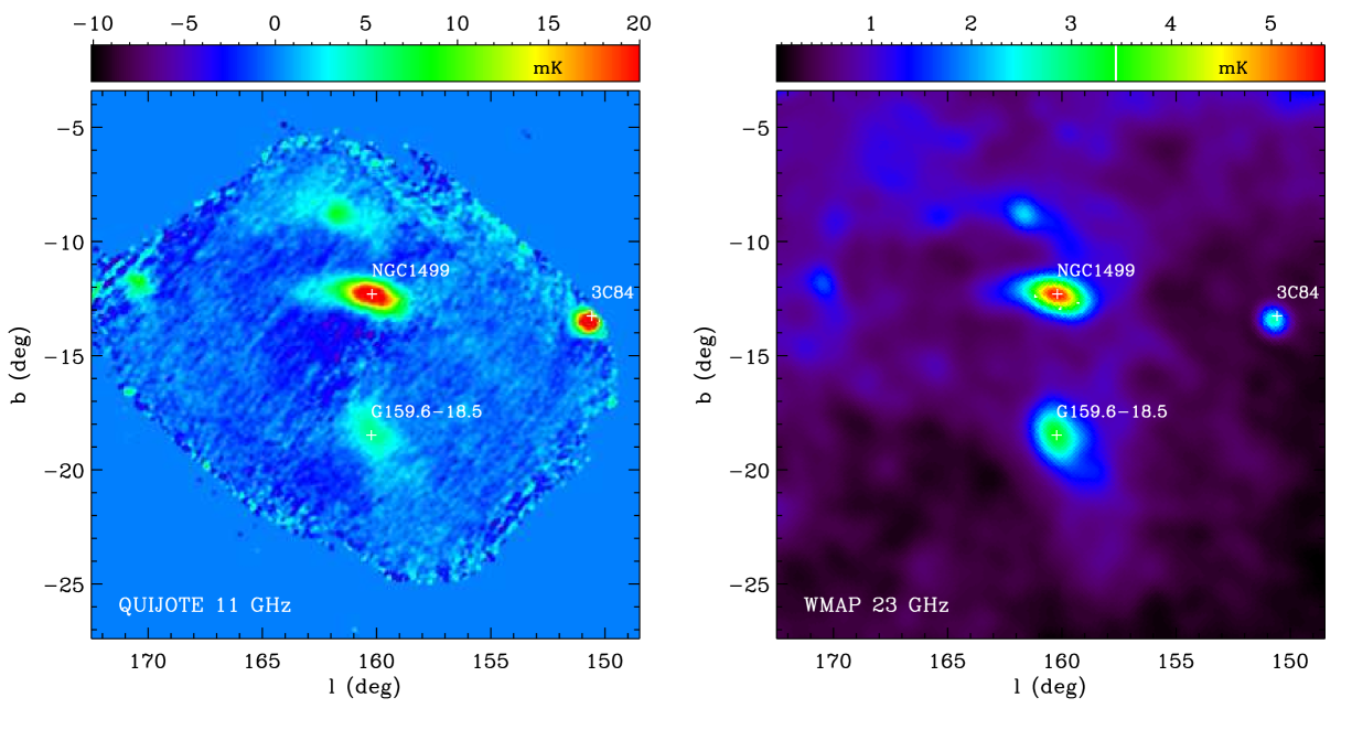
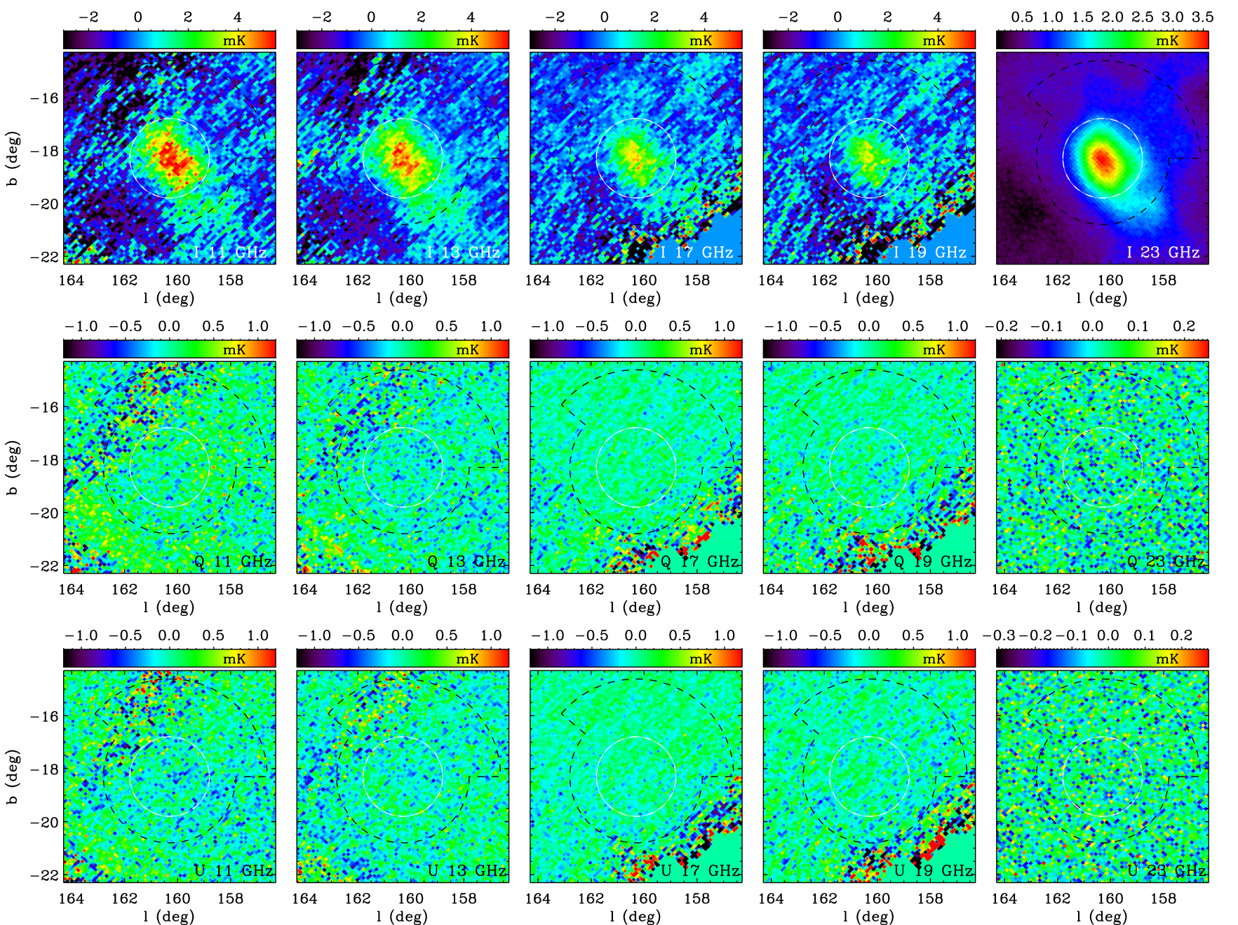
In Fig. 1 we show the intensity map at 11 GHz resulting from combining 149 h of observations, where emissions from G159.6-18.5, the California nebula (NGC1499) and the 3C84 quasar are clearly visible. More detailed , and maps at our four frequencies around the position of G159.6-18.5 are shown in Fig. 2. The and maps on this source are consistent with zero polarization, and therefore upper limits on the polarized intensity will be extracted in section 3.3. Some stripping is clearly visible in the maps, which is produced by the presence of regions with a higher noise due to a lower integration time per pixel and, to a lesser extent, to residuals. The inhomogenities in the coverage (integration time per pixel) maps are caused by the separation of the horns in the focal plane, which leads the sky coverage to be different when we observe the field before or after crossing the local meridian. In the and maps at 11 and 13 GHz of Fig. 2, the two orthogonal stripes with clearly higher noise correspond to regions with integration of s/pixel (pixel size 6.9 arcmin). By comparison, in the central region inside the circle where we perform the aperture photometry, the integration time is s/pixel, resulting in a lower pixel-to-pixel dispersion of the data.
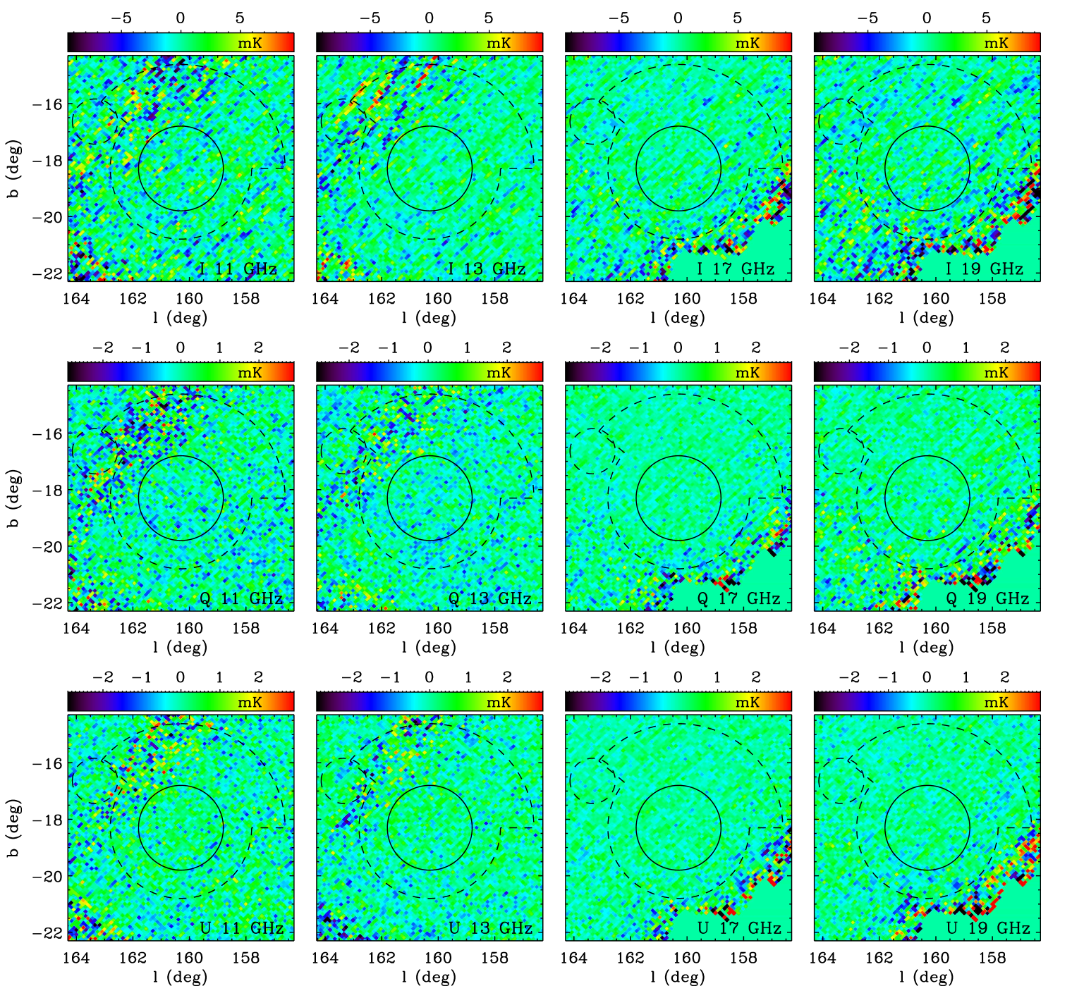
An important consistency test, that may reveal the presence of systematics and other spurious effects, is obtained through jackknife maps. We have uniformly split our full dataset in two halves in such a way that the maps of number of hits associated to these two halves are as similar as possible. The differences of the two halves divided by two, for the intensity and polarization maps at our four frequencies, are shown in Fig. 3. As expected, the intensity emission coming from G159.6-18.5 is consistently cancelled out in these maps. While a similar striping pattern to the maps in Fig. 2 is seen, these maps are dominated by instrumental noise. This is confirmed by the noise values shown in Table 1, where we compare the pixel-to-pixel RMS calculated in two different regions: the external ring that we will use for background subtraction when calculating the intensity and polarization fluxes, and a region of very low sky emission enclosed by the dashed circle represented in Fig. 3. The RMS values in and are similar in the original maps and in the sum and difference of the two halves. They are typically K/pixel (pixel size: 6.9 arcmin) or K/beam (beam size: degree). In the case of the maps, the RMS in the background ring are higher in the sum than in the difference because of the emission of the source. In the circle with low sky signal the values in the sum and in the difference maps are very similar.
The last column of Table 1 show the average RMS levels in the and maps normalized by the integration time per pixel. As the number of hits per pixel is very inhomogeneous, to calculate these numbers we have made a realization of Gaussian noise in which we assign to each pixel a noise proportional to , where is the integration time per pixel, and then calculate the pixel-to-pixel RMS. The amplitudes of the white-noise in the spectra of the time-ordered-data range between 898 K s1/2 (at 16.7 GHz) and 1228 K s1/2 (at 11.2 GHz)555Note that in this article we are using data from only two out of the four horns of QUIJOTE. Then, the global sensitivities of the experiment are a factor better, i.e. K s1/2, the number quoted in Section 2.1. residuals make the noises calculated on the maps only slightly higher, typically by a factor , confirming our previous statement that these maps are dominated by white (Gaussian) noise.
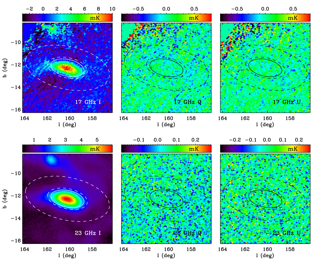
Another important consistency test for the presence of systematics, and in particular for the to polarization leakage, is to confirm that our polarization maps are consistent with noise in the position of unpolarized sources. This verification is provided by the nearby California HII region, which is also covered by our observations. As any standard HII region, it is dominated by free-free emission at the QUIJOTE frequencies, which is known to be practically unpolarized. In Fig. 4 we show intensity and polarization maps towards the California region, showing that the and maps are consistent with zero polarization.
3.2 Intensity SED
| Frequency | Flux | Flux density | Telescope/ |
|---|---|---|---|
| (GHz) | density (Jy) | residual (Jy) | survey |
| Haslam | |||
| Dwingeloo | |||
| Reich | |||
| COSMO. | |||
| QUIJOTE | |||
| COSMO. | |||
| QUIJOTE | |||
| COSMO. | |||
| COSMO. | |||
| QUIJOTE | |||
| QUIJOTE | |||
| WMAP | |||
| Planck | |||
| WMAP | |||
| WMAP | |||
| Planck | |||
| WMAP | |||
| Planck | |||
| WMAP | |||
| Planck | |||
| Planck | |||
| Planck | |||
| Planck | |||
| Planck | |||
| Planck | |||
| DIRBE | |||
| DIRBE | |||
| DIRBE |
As was indicated in section 2.2, we take the COSMOSOMAS fluxes for G159.6-18.5 from Planck Collaboration et al. (2011), which have already been corrected for the flux loss caused by the filtering of COSMOSOMAS data. While here we will use aperture photometry to derive our fluxes, in Planck Collaboration et al. (2014a) they were obtained by fitting the amplitude of an elliptical Gaussian with a fixed size of (FWHM). In a first-order approximation, the fluxes obtained through Gaussian fitting will be equivalent to those obtained from aperture photometry using a given aperture size. Therefore, in order to get a reliable intensity SED we choose a size for the aperture that gives the most similar fluxes to those presented in Planck Collaboration et al. (2011) for the Haslam et al. (1982), Berkhuijsen (1972), Reich & Reich (1986), WMAP , Planck and DIRBE maps (it must be noted that the WMAP and Planck maps used in this work correspond to a different release to that used in Planck Collaboration et al. (2011), but this will have a negligible effect). After trying different values, we found that a radius of gives the best agreement, with a very low reduced chi-squared of . The median of the background is computed in an external ring between and , which has the same area as the aperture. The derived fluxes in the QUIJOTE maps and in the other ancillary maps are listed in Table 2.
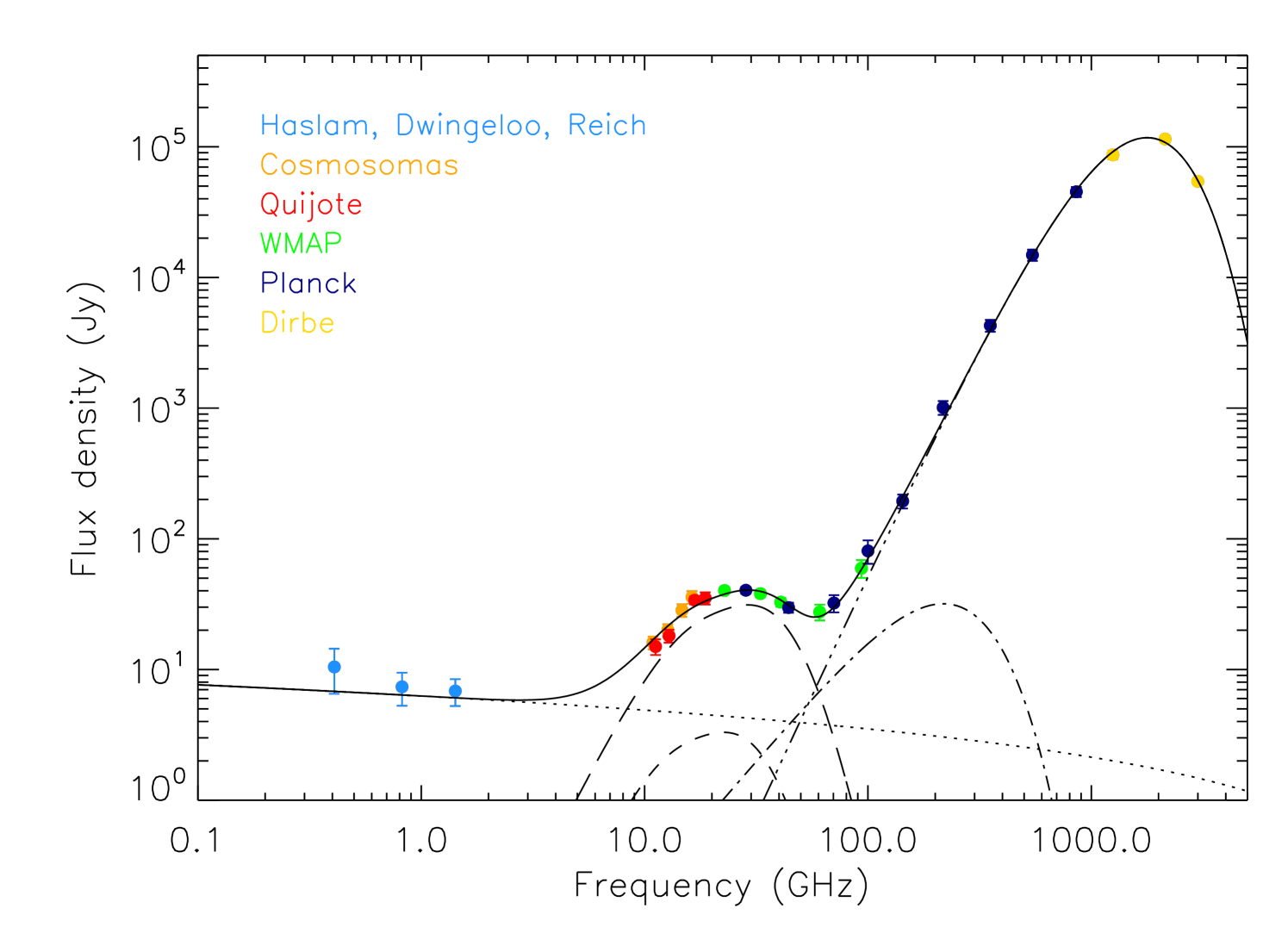
The final SED is depicted in Fig. 5, where the presence of AME clearly shows up at intermediate frequencies as an excess of emission over the other components. The intensities derived from these QUIJOTE observations trace, for the first time after the original measurements of the COSMOSOMAS experiment (Watson et al., 2005), the downturn of the spectrum at frequencies below GHz, as it is predicted by spinning dust models. In total, 13 data points are dominated by AME: the four QUIJOTE points, the four COSMOSOMAS points, the WMAP , and GHz frequencies and the Planck and GHz frequencies. We perform a joint multi-component fit to all the data, consisting of free-free emission, which dominates in the low-frequency tail, spinning dust, which dominates the intermediate frequencies, a CMB component, and thermal dust, which dominates the high-frequency end. As it was done in Planck Collaboration et al. (2011), to avoid possible CO residuals we exclude from the fit the 100 GHz and the 217 GHz values. We fix the spectrum of the free-free using the standard formulae shown in Planck Collaboration et al. (2011), with a value for the electron temperature typical of the solar neighbourhood, K, and fit for its amplitude, which is parameterized through the emission measure ().
Following Planck Collaboration et al. (2011), we consider a high-density molecular phase and a low-density atomic phase which produce spinning dust emission, and fit their respective amplitudes, which are given by the hydrogen column densities and . The CMB amplitude is denoted by , and would correspond to the average of the primordial CMB fluctuations in the aperture. Finally, the thermal dust is modelled as a single-component modified blackbody curve, , which depends on three parameters: the optical depth at m (), the emissivity spectral index () and the dust temperature (). Therefore, we jointly fit 7 parameters to all the data points: , , , , , and .
To define the spinning dust spectra of the molecular and atomic phases we use the spdust.2 code666http://www.tapir.caltech.edu/yacine/spdust/spdust.html (Ali-Haïmoud et al., 2009; Silsbee et al., 2011). Initially we use the same values as in Planck Collaboration et al. (2011) for the different parameters on which the spinning dust emissivity depends. This involves a modification of the code, as by default it uses nm and nm for the centroids of the two lognormal functions defining the dust grains size distributions, while the carbon abundance per hydrogen nucleus, , is selected from any of the values in table 1 of Weingartner & Draine (2001). Following Planck Collaboration et al. (2011), we use instead nm and nm, respectively for the molecular and atomic phases, and ppm. Using these two models, we get a good fit to our full dataset, with , where the spinning dust component is clearly dominated by the molecular phase, as was found by Planck Collaboration et al. (2011).
To analyze the possibility of the existence of slightly different spinning dust models that could provide a better fit to the data, we take the AME residual fluxes from the previous fit, and produce a grid of models varying some of the parameters of the molecular phase component. In particular, we vary: i) the hydrogen number density between 10 and 500 cm-3 with a step of 5 cm-3; ii) the kinetic gas temperature between 5 and 200 K in steps of 5 K; iii) the intensity of the radiation field relative to the average interstellar radiation field, for which we consider only the values and 2; iv) and the hydrogen ionization fraction, for which we consider the values , , and ppm. The best fit is obtained for and ppm, the same values used in Planck Collaboration et al. (2011). As the fit is very degenerate, to define the most-likely values for and we set Gaussian priors on four different parameters. First, we put soft priors on and centred on the same values used in Planck Collaboration et al. (2011), cm-3 and K, and with standard deviations cm-3 and K. An additional prior on can be derived from the canonical relation H cm (Finkbeiner et al., 2004). Using and from our best-fit model of the thermal dust component, we extrapolate the optical depth to m, and find H cm-2. We use this value to define the centre of the Gaussian prior, and H cm-2. Finally, the ratio between the hydrogen column density and the hydrogen volume density, , gives an estimate of the length along the line of sight of the spinning-dust-emitting region. We assume that this length might be of the order of the transverse angular size of the source. The source subtends an angle of around , which at the distance of the Perseus complex, 260 pc (Cernicharo et al., 1985), corresponds to 9.08 pc. We therefore set a fourth prior on this quantity defined by pc and pc.
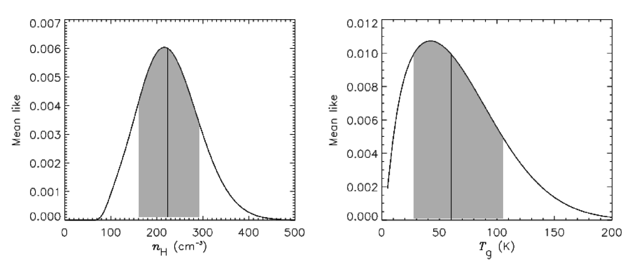
In Fig. 6 we show the marginalized likelihoods over and . We define the best-values for these parameters from the 50% integrals of the probability distribution, and the confidence intervals from the region encompassing the 68% of the area around those values. We get and K. As it was said before, the values of the intensity of the radiation field and of the hydrogen ionization fraction that maximize the likelihood are and ppm, respectively. We fix the other parameters of the molecular phase, and all the parameters corresponding to the atomic phase, to the same values that were used in Planck Collaboration et al. (2011). All these values are shown in Table 3. In this table, represents the ionized carbon fractional abundance, the molecular hydrogen fractional abundance, and the average dipole moment per atom. The meaning of the other parameters have been explained before in the text. We then obtain the corresponding spinning dust spectra for the molecular and atomic phases using these parameters as inputs for spdust.2. Fixing these spectra, we perform a joint fit of the five aforementioned components, obtaining the best-fit values for the 7 parameters defining these models, which are also shown in Table 3. We get , the same value as before, so we do not manage to improve the quality of the global fit after improving the spinning dust models. This highlights the difficulty of constraining the parameters on which the spinning dust emission depends due to the the strong degeneracies between them.
| (cm-6pc) | ||
|---|---|---|
| Molecular | Atomic | |
| (cm-3) | 30 | |
| 1 | 2 | |
| (K) | 100 | |
| (ppm) | 112 | 410 |
| (ppm) | 1 | 100 |
| 1 | 0.1 | |
| (nm) | ||
| (nm) | ||
| (ppm) | 68 | 68 |
| (D) | 9.34 | 9.34 |
| (1021 cm-2) | ||
| (K) | ||
| 1.73 0.11 | ||
| (K) | 18.2 0.6 | |
| ()10-4 | ||
| 0.99 | ||
The total hydrogen column density is H cm-2. This is a
bit higher than the expected value of H cm-2, which has been derived from the aforementioned
canonical relation, and extrapolating to using the fitted spectrum for the
thermal dust emission. The inferred lengths of the two spinning dust phases along the line of sight, , are
respectively pc and pc (a 68.3% C.L. upper bound is used here, as the
error bar is higher than the estimate). These values are of the order, or compatible, with the transverse
size of the region, pc. Our fitted values for and are consistent within 1-sigma with those derived in Planck Collaboration et al. (2011).
On the other hand, we get lower values for , and , but this is because these depend on the solid angle
subtended by the region. This value is a factor higher in our case, because we are using aperture photometry instead of
Gaussian fitting. When this factor is taken into account, then our values are brought into a better agreement with those of
Planck Collaboration et al. (2011). Finally, we find a positive value for , whereas in Planck Collaboration et al. (2011) it was negative. However, we have
checked that our value agrees with the average level of the CMB anisotropies within the aperture, which has been found to be
K in the Planck-DR1 CMB map resulting from the SMICA component separation method777Downloaded from the
Planck Legacy Archive, http://www.sciops.esa.int/index.php?project=planck&page=
Planck_Legacy_Archive. (Planck Collaboration et al., 2014d).
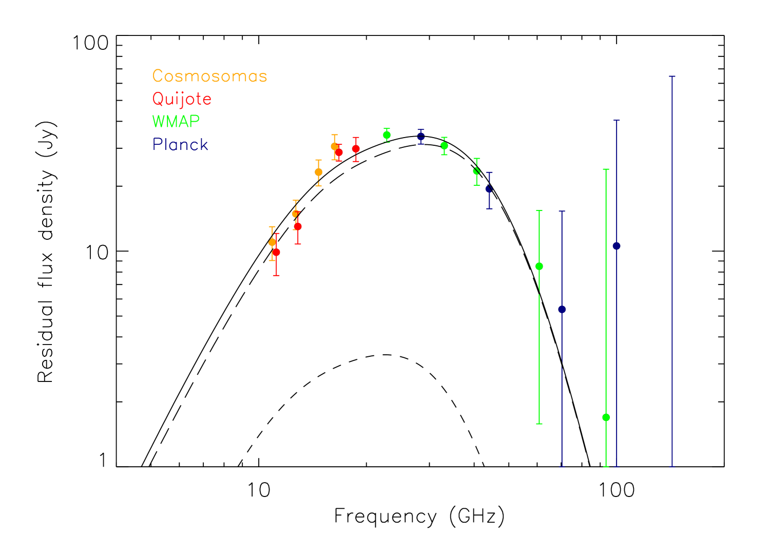
In Fig. 7 we show the residual spinning dust spectrum, obtained after subtracting the best-fit free-free, CMB and thermal dust components.
3.3 Polarization constraints
As no clear emission is seen in the and maps of Fig. 2, we derive upper limits on the polarization fraction of G159.6-18.5, following the procedure explained in section 2.3. In section 3.2 we defined the sizes of the aperture and of the background annulus so that we reproduced the fluxes in Planck Collaboration et al. (2011), which were obtained through Gaussian fitting. In order to minimize the error associated with the background subtraction, here we extend the size of the background annulus, and use a circular aperture with radius , and a background ring between and , with an extension towards the north-west as is shown in the maps of Fig. 2. At each frequency we calculate the RMS levels in this background annulus, to define the quantities that are introduced in equation 5 to calculate the errors on the Stokes parameters and . These errors, together with the fluxes resulting from the aperture photometry integration, are quoted in Table 4. Note that here the intensity fluxes in the QUIJOTE frequencies are slightly different to those presented in Table 2 owing to the different apertures. In order to get the AME residual fluxes shown in Table 4, using the new fluxes, we repeat the same fit that was performed in section 3.2, considering the same spinning dust spectra for the molecular and atomic phases.
It is important to point out that, as it became clear when we discussed the results of the jackknife tests in section 3.1, the uncertainties on the fluxes are here biased high because some extended emission of the source leaks into the background annulus. This does not have significant implications in our analysis as the uncertainty in the polarization fraction is driven by the errors in and .
The and fluxes shown in Table 4 are consistent with zero, and therefore we obtain de-biased (in section 2.3 we explained how this de-biasing is applied) upper limits at the 95% confidence level on the polarized intensity, . We also show in Table 4 upper limits at the 95% confidence level on the polarization fraction, taking as reference both the total intensity () and the residual AME intensity (). The values below the horizontal line in this table correspond to constraints obtained in maps that have been built by combining the two frequency bands of each horn. The most stringent upper limit we get on the polarization fraction is , and is obtained after combining the maps at 16.7 and 18.7 GHz. Due to the decrease of the intensity flux at lower frequencies, the constraints at 11.2 and 12.9 GHz are less stringent.
Note that, under the reliable assumption that the free-free emission is unpolarized (Rybicki & Lightman, 1979), any possible detection of polarization below GHz, where the thermal dust is clearly sub-dominant, should in principle be ascribed to AME. One caveat to this hypothesis is the possible presence of a Faraday Screen (FS) hosting a strong and regular magnetic field, which could induce a rotation of the background polarized emission. This idea was proposed by Reich & Reich (2009) to explain the high degree of polarization they detected towards G159.6-18.5 in observations from the Effelsberg telescope at 2.7 GHz. They suggest that this same mechanism could indeed be the responsible for the tentative polarized emission seen by Battistelli et al. (2006) at 11 GHz. Using as face value the rotation measure obtained by Reich & Reich (2009), RM rad m-2, López-Caraballo et al. (2011) estimated a polarization fraction of %, well below the upper limit at this frequency. Using this RM we estimate polarization fractions from the FS of and , respectively at 11 and 19 GHz. These values are well below our upper limits, while the value at 11 GHz is compatible with the measurement of Battistelli et al. (2006).
| (GHz) | (Jy) | (Jy) | (Jy) | (Jy) | (Jy) | (%) | (%) |
| 11.2 | 14.0 3.3 | 9.4 3.4 | -0.05 0.59 | -0.39 0.47 | |||
| 12.9 | 17.5 3.5 | 12.5 3.5 | 0.45 0.68 | -0.23 0.56 | |||
| 16.7 | 31.2 3.0 | 28.2 3.0 | 0.24 0.47 | -0.83 0.52 | |||
| 18.7 | 31.5 4.6 | 29.4 4.7 | -0.11 0.75 | 0.18 0.70 | |||
| 12.0 | 15.5 3.4 | 10.2 3.4 | 0.14 0.38 | -0.36 0.37 | |||
| 17.7 | 31.8 3.7 | 26.7 3.7 | 0.06 0.42 | -0.26 0.40 |
In section 3.1 we mentioned that one important consistency test for our data processing is the verification that it shows no polarization at the position of un-polarized sources like the California HII region. In Table 5 we show the corresponding , and fluxes, and derived upper limits on and , which have been obtained using the apertures shown in Fig. 4. The limits on the polarization fraction stand at the level of to (95% C.L.), depending on the frequency band. This constrains the possible existence of a leakage from intensity to polarization to values below this level. In fact, as it was mentioned in section 2.1, we expect the leakage to be below 0.3% ( dB). This number has been verified using observations of Cas A, where we recover a leakage pattern with a quadrupolar shape in the and maps, with a level of around (further details will be presented in separate technical papers).
| (GHz) | (Jy) | (Jy) | (Jy) | (Jy) | (%) |
|---|---|---|---|---|---|
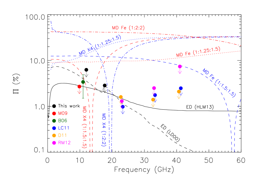
We plot our constraints, and previous results in the literature at different frequencies, in Fig. 8. It can be seen here that our observations fill the gap between previous results at frequencies below 11 GHz and above 20 GHz. The point at 9.65 GHz is an upper limit coming from GBT observations on LDN1622 (Mason et al., 2009). The value at 11 GHz represents the aforementioned tentative detection towards G159.6-18.5 at the level () of AME polarization from the COSMOSOMAS experiment (Battistelli et al., 2006), which is still consistent with our upper bound at GHz. The points at GHz come from WMAP 7-year data on the Perseus (López-Caraballo et al., 2011) and Ophiuchi (Dickinson et al. 2011, they also present results on Perseus) molecular clouds and on the HII region [LPH96] 201.663+1.643 (Rubiño-Martín et al. 2012b, they also show less-stringent constraints from the Pleiades reflection nebula and from the dark nebula LDN1622). Currently, the most stringent constraint is that obtained by López-Caraballo et al. (2011): at 23 GHz. This limit benefits from the fact that it is obtained at a frequency close to the peak ( GHz) of the AME in G159.6-18.5. The constraints on the polarization fraction from QUIJOTE come from a spectral region where the intensity flux density drops. However, according to the model of Hoang et al. (2013), the polarization fraction of the spinning dust emission peaks at GHz, and therefore observations at lower frequencies are more appropriate to constrain this model. All measurements, including ours, are consistent with this model, except maybe the previous limit from López-Caraballo et al. (2011) and that from Mason et al. (2009), which are slightly below.
Our upper limits on are not only affected by the decrease of AME flux at our frequencies, but also by the sparse sky coverage of our observations. We decided to survey an area large enough to cover the California HII region and also to get the source simultaneously in the four horns. Currently we are undertaking observations on a smaller area, centred in two individual horns, with the goal to increase by a factor the integration time per unit area. This would improve our map sensitivity by a factor , which would help push our current upper limits down to at GHz, and after combining the and GHz frequency bands, which is well below the polarization degree predicted by the Hoang et al. (2013) model at these frequencies. Furthermore, future observations at 30 GHz with the upcoming TGI experiment, which is expected to be 13 times more sensitive than the current MFI, will push these upper limits down by a significant amount.
However, it is important to note that the curve of the polarization degree obtained by Hoang et al. (2013) represents an upper limit. They inferred the alignment efficiency of interstellar dust grains from observations of the UV polarization excess towards two stars to predict the polarization degree of the spinning dust emission. In so doing they assumed that the UV polarization bump is produced exclusively by polycyclic aromatic hydrocarbon (PAHs) molecules, those which are thought to be responsible for spinning dust emission. However, if the graphite grains were also aligned, contributing to the UV polarization bump, then the alignment efficiency of PAHs could actually be lower and so would be the inferred degree of spinning dust polarization.
The previous model from Lazarian & Draine (2000) for spinning dust polarization is also plotted in Fig. 8, for the case of a cold neutral medium (CNM), together with different models from Draine & Lazarian (1999) predicting the degree of polarization of the magnetic dipole emission for different grain shapes and compositions. In particular, we show the cases of grains made of metallic Fe, and of the hypothetical material X4 defined in Draine & Lazarian (1999). Concerning the grain geometries, different axial ratios :: are shown, as indicated in the figure. All these models predict polarization fractions typically above , much higher than that of the spinning dust emission, and are ruled out by our and previous observations. However, it must be noted that these models consider the dust grains to have a perfect ordering of the atomic magnetic moments in a single domain. A more realistic case considering randomly-oriented single-domain magnetic inclusions has been recently studied by Draine & Hensley (2013), resulting in much lower polarization degrees, of the order of in the range GHz, or below.
4 Conclusions
We have presented the first results obtained with the QUIJOTE experiment, a new polarimeter aimed at measuring the B-mode anisotropy from inflation and also at characterizing the polarized foregrounds at low frequencies. These results are based on observations of the Perseus molecular complex, one of the regions where the AME has extensively been studied. Our observations cover G159.6-18.5, the region where AME is produced, and the California HII region. Our intensity data on G159.6-18.5 traces the decrease of the flux of this source at frequencies below GHz, confirming the prediction of the models based on spinning dust radiation, which currently are the best at reproducing the frequency spectrum of the AME. This confirms previous results on this region obtained with the COSMOSOMAS experiment (Watson et al., 2005). When combining the QUIJOTE measurements with data coming from COSMOSOMAS, WMAP-9yr and Planck-DR1, we get an intensity SED with 13 points between 10 and 50 GHz being dominated by AME, providing what probably is the most precise spectrum of this emission ever measured in an individual object. This intensity SED is well fitted () by a combination of free-free, CMB, spinning dust and thermal dust, and two spinning dust components associated to a high-density molecular phase and to a low-density atomic phase. We attempt to fit some of the parameters describing the physical environment of the cloud, and which define the shape of the spinning dust spectrum, but the solution is clearly degenerate and this approach does not achieve a better fit. However, with the physical parameters we use for the spinning dust spectra, we get reliable values for the 7 parameters of our model.
The California HII region is well detected in intensity, presenting a spectrum at QUIJOTE frequencies consistent with free-free emission. The polarization maps at the position of California are consistent with noise, as it is expected for regions dominated by free-free emission, which is very lowly polarized. No polarization is detected at the position of G159.6-18.5 either, so then we extract upper limits on the polarized intensity and on its degree of polarization. After combining the low-frequency and high-frequency maps of two horns of QUIJOTE, we get and ( C.L.), respectively at and GHz, being the first upper limits on the AME polarization fraction in this frequency range. These constraints are consistent with models of the spinning dust emission, that predict polarization fractions between and in this frequency range, and rule out several models based on magnetic dipole emission. Pushing these constraints even further is crucial to test the theoretical models and also to assess up to what level AME will hinder the detection of the B-mode signal by current and future experiments operating in the frequency range 10 to 80 GHz. New QUIJOTE observations in this region will improve the sensitivity in our maps so that we will be able to improve the previous constraints at least by a factor 2, allowing to reach a sensitivity on the polarization fraction close to the predictions of the spinning dust models.
Acknowledgments
This work has been partially funded by the Spanish Ministry of of Economy and Competitiveness (MINECO) under the projects AYA2007-68058-C03-01, AYA2010-21766-C03-02, and the Consolider-Ingenio project CSD2010-00064 (EPI: Exploring the Physics of Inflation). CD acknowledges support from an ERC Starting (Consolidator) Grant (no. 307209). SH acknowledges support from an STFC-funded studentship. We acknowledge the use of data from the Planck/ESA mission, downloaded from the Planck Legacy Archive, and of the Legacy Archive for Microwave Background Data Analysis (LAMBDA). Support for LAMBDA is provided by the NASA Office of Space Science. Some of the results in this paper have been derived using the HEALPix (Górski et al., 2005) package.
References
- Ali-Haïmoud et al. (2009) Ali-Haïmoud, Y., Hirata, C. M., & Dickinson, C. 2009, MNRAS, 395, 1055
- AMI Consortium et al. (2009) AMI Consortium, Scaife, A. M. M., Hurley-Walker, N., et al. 2009, MNRAS, 400, 1394
- Battistelli et al. (2006) Battistelli, E. S., Rebolo, R., Rubiño-Martín, J. A., et al. 2006, ApJ, 645, L141
- Bennett et al. (2013) Bennett, C. L., Larson, D., Weiland, J. L., et al. 2013, ApJS, 208, 20
- Berkhuijsen (1972) Berkhuijsen, E. M. 1972, A&AS, 5, 263
- BICEP1 Collaboration et al. (2014) BICEP1 Collaboration, Barkats, D., Aikin, R., Bischoff, C., et al. 2014, ApJ, 783, 67
- BICEP2 Collaboration et al. (2014) BICEP2 Collaboration, Ade, P. A. R., Aikin, R. W., Barkats, D., et al. 2014, Physical Review Letters, 112, 241101
- Casassus et al. (2006) Casassus, S., Cabrera, G. F., Förster, et al. 2006, ApJ, 639, 951
- Casassus et al. (2008) Casassus, S., Dickinson, C., Cleary, K., et al. 2008, MNRAS, 391, 1075
- Cernicharo et al. (1985) Cernicharo, J., Bachiller, R., & Duvert, G. 1985, A&A, 149, 273
- Davies et al. (2006) Davies, R. D., Dickinson, C., Banday, A. J., et al. 2006, MNRAS, 370, 1125
- Dickinson et al. (2009) Dickinson, C., Davies, R. D., Allison, J. R., et al. 2009, ApJ, 690, 1585
- Dickinson et al. (2011) Dickinson, C., Peel, M., & Vidal, M. 2011, MNRAS, 418, L35
- Draine & Lazarian (1998) Draine, B. T., & Lazarian, A. 1998, ApJ, 508, 157
- Draine & Lazarian (1999) Draine, B. T., & Lazarian, A. 1999, ApJ, 512, 740
- Draine & Hensley (2013) Draine, B. T., & Hensley, B. 2013, ApJ, 765, 159
- Femenia et al. (1998) Femenia, B., Rebolo, R., Gutierrez, C. M., Limon, M., & Piccirillo, L. 1998, ApJ, 498, 117
- Finkbeiner et al. (2002) Finkbeiner, D. P., Schlegel, D. J., Frank, C., & Heiles, C. 2002, ApJ, 566, 898
- Finkbeiner et al. (2004) Finkbeiner, D. P., Langston, G. I., & Minter, A. H. 2004, ApJ, 617, 350
- Flauger et al. (2014) Flauger, R., Hill, J. C., & Spergel, D. N. 2014, arXiv:1405.7351
- García-Lorenzo et al. (2010) García-Lorenzo, B., Eff-Darwich, A., Castro-Almazán, J., et al. 2010, MNRAS, 405, 2683
- Génova-Santos et al. (2011) Génova-Santos, R., Rebolo, R., Rubiño-Martín, J. A., López-Caraballo, C. H., & Hildebrandt, S. R. 2011, ApJ, 743, 67
- Górski et al. (2005) Górski, K. M., Hivon, E., Banday, A. J., et al. 2005, ApJ, 622, 759
- Hafez et al. (2008) Hafez, Y. A., Davies, R. D., Davis, R. J., et al. 2008, MNRAS, 388, 1775
- Hauser et al. (1998) Hauser, M. G., Arendt, R. G., Kelsall, T., et al. 1998, ApJ, 508, 25
- Haslam et al. (1982) Haslam, C. G. T., Salter, C. J., Stoffel, H., & Wilson, W. E. 1982, A&AS, 47, 1
- Hoang et al. (2010) Hoang, T., Draine, B. T., & Lazarian, A. 2010, ApJ, 715, 1462
- Hoang et al. (2013) Hoang, T., Lazarian, A., & Martin, P. G. 2013, ApJ, 779, 152
- Kamionkowski et al. (1997) Kamionkowski, M., Kosowsky, A., & Stebbins, A. 1997, Phys.Rev.D, 55, 7368
- Kogut et al. (1996a) Kogut, A., Banday, A. J., Bennett, C. L., et al. 1996a, ApJ, 460, 1
- Kogut et al. (1996b) Kogut, A., Banday, A. J., Bennett, C. L., et al. 1996b, ApJ, 464, L5
- Lazarian & Draine (2000) Lazarian, A., & Draine, B. T. 2000, ApJ, 536, L15
- Leitch et al. (1997) Leitch, E. M., Readhead, A. C. S., Pearson, T. J., & Myers, S. T. 1997, ApJ, 486, L23
- López-Caraballo et al. (2011) López-Caraballo, C. H., Rubiño-Martín, J. A., Rebolo, R., & Génova-Santos, R. 2011, ApJ, 729, 25
- Macellari et al. (2011) Macellari, N., Pierpaoli, E., Dickinson, C., & Vaillancourt, J. E. 2011, MNRAS, 418, 888
- Mason et al. (2009) Mason, B. S., Robishaw, T., Heiles, C., Finkbeiner, D., & Dickinson, C. 2009, ApJ, 697, 1187
- Mather et al. (1999) Mather, J. C., Fixsen, D. J., Shafer, R. A., Mosier, C., & Wilkinson, D. T. 1999, ApJ, 512, 511
- Mortonson & Seljak (2014) Mortonson, M. J., & Seljak, U. 2014, arXiv:1405.5857
- Murphy et al. (2010) Murphy, E. J., Helou, G., Condon, J. J., et al. 2010, ApJ, 709, L108
- Planck Collaboration et al. (2011) Planck Collaboration. Planck Early Results XX, 2011, A&A, 536, A20
- Planck Collaboration et al. (2014a) Planck Collaboration. Planck Intermediate Results XXV, 2014a, A&A, 565, AA103
- Planck Collaboration et al. (2014b) Planck Collaboration. Planck Intermediate Results XXX, 2014b, arXiv:1409.5738
- Planck Collaboration et al. (2014c) Planck Collaboration. Planck 2013 Resuls I, 2014c, A&A, 571, AA1
- Planck Collaboration et al. (2014d) Planck Collaboration. Planck 2013 Resuls XII, 2014d, A&A, 571, AA12
- Planck Collaboration et al. (2014e) Planck Collaboration. Planck 2013 Resuls XIII, 2014e, A&A, 571, AA13
- QUIET Collaboration et al. (2012) QUIET Collaboration, Araujo, D., Bischoff, C., et al. 2012, ApJ, 760, 145
- de Oliveira-Costa et al. (1998) de Oliveira-Costa, A., Tegmark, M., Page, L. A., & Boughn, S. P. 1998, ApJ, 509, L9
- de Oliveira-Costa et al. (1999) de Oliveira-Costa, A., Tegmark, M., Gutierrez, C. M., et al. 1999, ApJ, 527, L9
- Platania et al. (2003) Platania, P., Burigana, C., Maino, D., et al. 2003, A&A, 410, 847
- (50) Rebolo, R., et al. in preparation
- Reich & Reich (1986) Reich, P., & Reich, W. 1986, A&AS, 63, 205
- Reich & Reich (2009) Reich, W., & Reich, P. 2009, IAU Symposium, 259, 603
- Rybicki & Lightman (1979) Rybicki, G. B., & Lightman, A. P. 1979, Radiative Processes in Astrophysics, John Wiley & Sons
- Rubiño-Martín et al. (2012a) Rubiño-Martín, J. A., Rebolo, R., Aguiar, M., et al. 2012a, Society of Photo-Optical Instrumentation Engineers (SPIE) Conference Series, 8444
- Rubiño-Martín et al. (2012b) Rubiño-Martín, J. A., López-Caraballo, C. H., Génova-Santos, R., & Rebolo, R. 2012b, Advances in Astronomy, 351836
- Silsbee et al. (2011) Silsbee, K., Ali-Haïmoud, Y., & Hirata, C. M. 2011, MNRAS, 411, 2750
- Tibbs et al. (2010) Tibbs, C. T., Watson, R. A., Dickinson, C., et al. 2010, MNRAS, 402, 1969
- Tibbs et al. (2013) Tibbs, C. T., Scaife, A. M. M., Dickinson, C., et al. 2013, ApJ, 768, 98
- Vaillancourt (2006) Vaillancourt, J. E. 2006, PASP, 118, 1340
- Vidal et al. (2011) Vidal, M., Casassus, S., Dickinson, C., et al. 2011, MNRAS, 414, 2424
- Watson et al. (2005) Watson, R. A., Rebolo, R., Rubiño-Martín, et al. 2005, ApJ, 624, L89
- Weiland et al. (2011) Weiland, J. L., Odegard, N., Hill, R. S., et al. 2011, ApJS, 192, 19
- Weingartner & Draine (2001) Weingartner, J. C., & Draine, B. T. 2001, ApJ, 548, 296
- Ysard & Verstraete (2010) Ysard, N., & Verstraete, L. 2010, A&A, 509, AA12
- Zaldarriaga & Seljak (1997) Zaldarriaga, M., & Seljak, U. 1997, Phys.Rev.D, 55, 1830