Measuring Hubble constant using localized and unlocalized fast radio bursts
Abstract
Hubble constant () is one of the most important parameters in the standard model. The measurements given by two major methods show a gap greater than , also known as Hubble tension. Fast radio bursts (FRBs) are extragalactic events with millisecond duration, which can be used as cosmological probes with high accuracy. In this paper, we constrain the Hubble constant using localized and unlocalized FRBs. The probability distributions of and from IllustrisTNG simulation are used. 69 localized FRBs give the constraint of , which lies between early-time and late-time values, thus highlighting its individuality as a cosmological probe. We also use Monte Carlo simulation and direct sampling to calculate the pseudo redshift distribution of 527 unlocalized FRBs from CHIME observation. The median values and fixed scattered pseudo redshifts are both used to constrain Hubble constant. The corresponding constraints of from unlocalized bursts are and respectively. This result also indicates that the uncertainty of Hubble constant constraint will drop to if the number of localized FRBs is raised to . Above uncertainties only include the statistical error. The systematic errors are also discussed, and play the dominant role for the current sample.
keywords:
cosmological parameters – fast radio bursts1 Introduction
The Lambda Cold Dark Matter () model, also known as the standard model of cosmology, has provided convincing explanations for numerous cosmological observation facts. consists of six basic cosmological parameters with more derived parameters including Hubble constant (). As one of the most fundamental parameters in cosmology, describes the expansion rate of current universe (Hubble, 1929), and its reciprocal 1/ gives an estimation on the age of the universe. Constraints on Hubble constant have been made with generally two distinct methods (Freedman, 2021), early time probes given by Cosmic Microwave Background (CMB) and late time probes given by stars such as Cepheid-calibrated type Ia supernovae (SNe Ia). With rapidly developing telescopes, predictions given by both methods have shown increased accuracy. Planck Collaboration et al. (2020) gave prediction of based on Planck cosmic microwave background power spectra with 68% confidence, while Riess et al. (2022) showed with Cepheid-SNIa sample. A non-negligible gap of more than 4 appears between both results, which is known as the "Hubble Tension" (Valentino et al., 2021; Hu & Wang, 2023). It is crucial to find an independent approach to resolve the Hubble tension.
Fast radio bursts (FRBs) are extraordinarily bright radio bursts first discovered in 2007 (Lorimer et al., 2007). With subsequent discoveries of five FRBs in several years (Keane et al., 2012; Thornton et al., 2013), FRB is universally acknowledged as a special kind of high-energy astronomical phenomena characterized by extremely high burst energy, millisecond duration and extragalactic origin (Xiao et al., 2021; Petroff et al., 2022; Zhang, 2023; Wu & Wang, 2024). The mechanism of FRBs remains unknown, despite different hypotheses of its origination. Still, it has been proved that almost all FRBs are originated outside Milky Way due to extraordinary burst rate and extragalactic dispersion measures (Cordes & Chatterjee, 2019). Some FRBs are observed multiple times while others have not shown repetitiveness for now. FRBs occur at an extreme rate, and with more telescopes searching for FRBs, observed FRBs are significantly increasing while a small yet growing proportion of FRBs are well localized with host galaxy and a definite redshift .
To employ FRBs as cosmological probes, dispersion measure (DM) is a characteristic property defined as the integral of electron number density along the path of propagation, i.e. DM=d. By precisely determining DM, especially component contributed by intergalactic medium (), FRBs could be used as high-accuracy probes in multiple cases (Bhandari & Flynn, 2021; Wu & Wang, 2024), such as measuring the Hubble constant (Wu et al., 2022; Hagstotz et al., 2022; James et al., 2022; Zhao et al., 2022; Wei & Melia, 2023; Gao et al., 2024) and Hubble parameter (Wu et al., 2020), dark energy (Zhou et al., 2014; Walters et al., 2018; Kumar & Linder, 2019; Qiu et al., 2022), and bounding the photon rest mass (Wang et al., 2021; Lin et al., 2023; Wang et al., 2024), measuring reionization history (Zhang et al., 2021; Bhattacharya et al., 2021), probing compact dark matter (Muñoz et al., 2016; Wang & Wang, 2018), and finding missing baryons (Walters et al., 2018; Li et al., 2020; Macquart et al., 2020a; Yang et al., 2022; Lin & Zou, 2023; Wang & Wei, 2023; Connor et al., 2024). Early researches assume dispersion measures contributed by intergalactic medium () and host galaxy () to be certain values, though it is practically not possible to distinguish the partition between and . Macquart et al. (2020b) and Zhang et al. (2021) provided a possible solution of considering the probability density distributions for and to solve "degeneracy problem". Several works have been done to constrain with FRBs, such as Wu et al. (2022) using 18 localized bursts to get a constraint of 8% uncertainty, Hagstotz et al. (2022) measuring from localized FRBs assuming a constant value of , James et al. (2022) using data from Australian Square Kilometer Array Pathfinder and Parkes to get a result of 10.9% uncertainty, Zhao et al. (2022) using 12 unlocalized FRBs to constrain by identifying host galaxies with probability distributions, and Kalita et al. (2024) using 64 localized FRBs to constrain with different models of IGM and host galaxy.
In this paper, we constrain Hubble constant with 69 localized FRBs and 527 unlocalized FRBs, and predict the confidence interval of Hubble constant assuming all 527 FRBs are well localized. In Section 2 we introduce the theoretical model used for DMs of FRBs. In Section 3 we show our Markov Chain Monte Carlo model and give the constraint given by localized FRBs. In Section 4 we propose the pseudo redshift of unlocalized FRBs and give corresponding result. In Section 5 we discuss the statistical and systematic error of our result.
2 Distribution of dispersion measures
Generally, the dispersion measures of FRBs could be broken down into following components:
| (1) |
where is total observed DM, while , , and refers to DM contributed by interstellar medium (ISM) within Milky Way, galactic halo, intergalactic medium and host galaxy of FRB respectively.
2.1 Galactic dispersion measures
The former two components, and , are contributed by medium within Milky Way and also referred to as a whole, i.e. . could be well described by galactic electron distribution models such as YMW16 by Yao et al. (2017) and NE2001 by Cordes & Lazio (2002). According to Ocker et al. (2021), YMW16 might overestimate for FRBs in the direction of anticenter and possibly other low-latitude bursts. The difference between NE2001 and YMW16 may have little influence on constraint of (Wu et al., 2022), still we apply NE2001 to estimate as previous researchers do. Prochaska & Zheng (2019) gave the constraint of = 5080 based on multiple observation data. It is reasonable to assume that follows a Gaussian distribution with = 65 and . To reduce calculation and avoid another level of integration, we simplify to be its mean value, i.e. = 65 , which should have minor influence on our estimation since the halo component appears as linear form in .
2.2 Extragalactic dispersion measures
As discussed in Section 2.1, contributions from within our Galaxy can be well estimated with galactic electron models, we subtract from total DM to obtain the extragalactic component:
| (2) |
is the dispersion measure contributed by host galaxy of FRB source, and its probability distribution can be fitted by a lognormal distribution according to Macquart et al. (2020b). The intergalactic component could be described with a Gaussian-like distribution around its mean value. In a standard universe model, the mean value of is given by Deng & Zhang (2014) as:
| (3) |
where is proton mass, is the fraction of baryon in IGM. Previous researches prefer a value of according to Shull et al. (2012), yet Connor et al. (2024) gives a more accurate constraint of with data from the Deep Synoptic Array (DSA-110) using both FRB and non-FRB methods (notably what we called corresponds to instead of in their research). We adopt the value of in our simulation. The integral is defined as:
| (4) |
The cosmological parameters and are given by Planck 2018 results (Planck Collaboration et al., 2020), and we have assuming a flat universe. is decided as an assumption in Planck results based on big bang nucleosynthesis (BBN) constraints and primordial deuterium abundance measurements by Cooke et al. (2018), which is always given in the form of where , thus we modify the equation to keep in the form of . and in Equation (4) are hydrogen and helium fractions normalized to 0.75 and 0.25 respectively, which can be neglected as . and are ionization fraction of hydrogen and helium, which could also be considered to be at . Equations (3) and (4) can now be further rewritten as:
| (5) |
3 Monte Carlo simulation and constraint with localized FRBs
3.1 Monte Carlo simulation
To run a Markov Chain Monte Carlo (MCMC) simulation, the probability distribution of extragalactic DM components must be calculated. As described in Section 2.2, follows a lognormal distribution while can be fitted with a Gaussian-like distribution, which often writes as (McQuinn, 2013; Macquart et al., 2020b):
| (6) |
| (7) |
where and are parameters indicating inner density profile of halo gas, and Macquart et al. (2020b) proposed the best-fitting result of . and are normalization parameters given by and , while , and are distribution parameters respectively. is generally chosen as distribution parameter instead of , since indicates mean value of .
One possible way of further simulation to determine is to fit all undetermined parameters at the same time, and the probability function goes like:
| (8) |
Still, since the number of localized FRBs is limited (), the confidence may be weakened to fit a four-dimensional parameter space with current data. Another concern is that distribution parameters are not fixed constant for different FRBs, and some have shown redshift-dependent. Zhang et al. (2020) and Zhang et al. (2021) proposed the best-fitted distribution parameters of and derived from IllustrisTNG Simulation (Pillepich et al., 2017), which takes redshift-dependent evolution into consideration as well. Zhang et al. (2021) also provided the evolution of and , and it is shown that the best-fitted value slightly deviates from normalization. To apply results above, all localized FRBs are divided roughly into three categories based on host galaxy: (a) non-repeating (one-off) bursts; (b) FRB121102-like repeating bursts: host galaxy stellar mass , star formation rate (SFR) ; (c) FRB180916-like repeating bursts: host galaxy stellar mass , SFR . Note that this classification only indicates qualitative properties of the host galaxy and is not absolute. Zhang et al. (2020) and Zhang et al. (2021) provided best-fitted values of distribution parameters at several typical redshifts, and we perform a monotone cubic spline interpolation for each parameter to obtain values at any given redshift.
By obtaining values for from IllustrisTNG, the only free parameter left is , which is what we are interested in. Taking all parameters into Equation (6) and (7), we have the likelihood function for any single FRB:
| (9) | ||||
Though not wrote explicitly, the distribution parameters in Equation (9) are distinct for each burst. For the FRB, the complete likelihood function is:
| (10) |
and the total log-likelihood function of all FRBs is:
| (11) |
According to Bayesian theory, we still need a prior of to perform parameter estimation, and we use a uniform distribution as its prior.
3.2 Simulation of localized FRBs
3.2.1 Data preprocessing
| FRB Type | TNS Name | RA | DEC | DM () | Redshift | Reference |
|---|---|---|---|---|---|---|
| 1 | FRB20121102 | 5:31:58 | +33:08:04 | 557 | 0.1927 | Tendulkar et al. (2017) |
| Chatterjee et al. (2017) | ||||||
| 1 | FRB20180301 | 6:12:54.44 | +4:40:15.8 | 536 | 0.3304 | Bhandari et al. (2022) |
| 2 | FRB20180916 | 1:58:00.75 | +65:43:00.32 | 348.76 | 0.0337 | Marcote et al. (2020) |
| 3 | FRB20180924 | 21:44:25.3 | -40:54:00.1 | 361.42 | 0.3214 | Bannister et al. (2019) |
| 1 | FRB20181030 (Unused) | 10:34:20.1 | +73:45:05 | 103.5 | 0.0039 | Bhardwaj et al. (2021) |
| 2 | FRB20180814 | 4:22:56.01 | +73:39:40.7 | 189.4 | 0.068 | Michilli et al. (2023) |
| 3 | FRB20181112 | 21:49:23.63 | -52:58:15.39 | 589.27 | 0.4755 | Prochaska et al. (2019) |
| 3 | FRB20190102 | 21:29:39.76 | -79:28:32.5 | 364.5 | 0.2913 | Bhandari et al. (2020) |
| 1 | FRB20190303A | 13:51:58 | +48:7:20 | 222.4 | 0.064 | Michilli et al. (2023) |
| 3 | FRB20190523 | 13:48:15.6 | +72:28:11 | 760.8 | 0.66 | Ravi et al. (2019) |
| 3 | FRB20190608 | 22:16:04.74 | -7:53:53.6 | 339.5 | 0.11778 | Chittidi et al. (2021) |
| 3 | FRB20190611 | 21:22:58.91 | -79:23:51.3 | 321.4 | 0.378 | Heintz et al. (2020) |
| 3 | FRB20190614 | 4:20:18.13 | +73:42:22.9 | 959.2 | 0.6 | Law et al. (2020) |
| 1 | FRB20190711 | 57:40.7 | -80:21:28.8 | 593.1 | 0.522 | Heintz et al. (2020) |
| 3 | FRB20190714 | 12:15:55.12 | -13:01:15.7 | 504.13 | 0.2365 | Heintz et al. (2020) |
| 3 | FRB20191001 | 21:33:24.373 | -54:44:51.43 | 507.9 | 0.234 | Heintz et al. (2020) |
| 3 | FRB20191228 | 22:57:43.3 | -29:35:38.7 | 297.5 | 0.2432 | Bhandari et al. (2022) |
| 3 | FRB20200430 | 15:18:49.54 | +12:22:36.8 | 380.25 | 0.16 | Heintz et al. (2020) |
| 3 | FRB20200906 | 3:3:59.08 | -14:04:59.5 | 577.8 | 0.3688 | Bhandari et al. (2022) |
| 2 | FRB20201124 | 5:08:03.5 | +26:03:38.4 | 413.52 | 0.098 | Ravi et al. (2022) |
| 1 | FRB20190520B (Unused) | 16:02:04.266 | -11:17:17.33 | 1210.3 | 0.241 | Niu et al. (2022) |
| 3 | FRB20200120E (Unused) | 9:57:54.7 | +68:49:0.9 | 87.8 | 0.0008 | Kirsten et al. (2022) |
| 3 | FRB20210117A | 22:39:55.015 | -16:09:05.45 | 728.95 | 0.214 | Bhandari et al. (2023) |
| 3 | FRB20220610A | 23:24:17.569 | -33:30:49.37 | 1457.624 | 1.016 | Ryder et al. (2023) |
| 2 | FRB20220912A | 23:09:04.9 | +48:42:25.4 | 219.46 | 0.0771 | Ravi et al. (2023b) |
| 3 | FRB20220319D (Unused) | 08:42.7 | +71:02:06.9 | 110.95 | 0.0111 | Ravi et al. (2023a) |
| 3 | FRB20210410D | 21:44:20.7 | -79:19:05.5 | 578.78 | 0.1415 | Caleb et al. (2023) |
| 3 | FRB20210405I (Unused) | 17:01:21.5 | -49:32:42.5 | 565.17 | 0.066 | Driessen et al. (2023) |
| 3 | FRB20220207C | 20:40:47.886 | +72:52:56.378 | 262.38 | 0.04304 | Law et al. (2024) |
| 3 | FRB20220307B | 23:23:29.88 | +72:11:32.6 | 499.27 | 0.248123 | Law et al. (2024) |
| 3 | FRB20220310F | 8:58:52.9 | +73:29:27.0 | 462.24 | 0.477958 | Law et al. (2024) |
| 3 | FRB20220418A | 14:36:25.34 | +70:05:45.4 | 623.25 | 0.622 | Law et al. (2024) |
| 3 | FRB20220506D | 21:12:10.76 | +72:49:38.2 | 396.97 | 0.30039 | Law et al. (2024) |
| 3 | FRB20220509G | 18:50:40.8 | +70:14:37.8 | 269.53 | 0.0894 | Law et al. (2024) |
| 3 | FRB20220825A | 20:47:55.55 | +72:35:05.9 | 651.24 | 0.241397 | Law et al. (2024) |
| 3 | FRB20220914A | 18:48:13.63 | +73:20:12.9 | 631.28 | 0.1139 | Law et al. (2024) |
| 3 | FRB20220920A | 16:01:01.70 | +70:55:07.7 | 314.99 | 0.158239 | Law et al. (2024) |
| 3 | FRB20221012A | 18:43:11.69 | +70:31:27.2 | 441.08 | 0.284669 | Law et al. (2024) |
| 3 | FRB20210603A | 0:41:05.774 | +21:13:34.573 | 500.147 | 0.177 | Cassanelli et al. (2023) |
| 3 | FRB20210320C | - | - | 384.8 | 0.2797 | Shannon(in prep.) |
| 3 | FRB20211127I | - | - | 234.83 | 0.0469 | Deller(in prep.) |
| FRB Type | TNS Name | RA | DEC | DM () | Redshift | Reference |
| 3 | FRB20211212A | - | - | 206 | 0.0715 | Deller(in prep.) |
| 1 | FRB20240114A | 21:27:39.835 | +4:19:45.634 | 527.7 | 0.13 | Chen(in prep.) |
| 3 | FRB20171020A | 22:15:24.75 | -19:35:07.00 | 114.1 | 0.0087 | Mahony et al. (2018) |
| 3 | FRB20201123A (Unused) | 17:34:40.8 | -50:40:12 | 433.55 | 0.0507 | Rajwade et al. (2022) |
| 3 | FRB20210807D | 19:56:53.14 | -00:45:44.50 | 251.3 | 0.1293 | Deller(in prep.) |
| 3 | FRB20211203C | 13:38:15.00 | -31:22:48.20 | 635 | 0.3439 | Gordon et al. (2023) |
| 3 | FRB20220105A | 13:55:12.94 | +22:27:59.40 | 580 | 0.2785 | Gordon et al. (2023) |
| 1 | FRB20220529A | 01:16:25.01 | +20:37:57.03 | 246 | 0.183900 | Li(in prep.) |
| 3 | FRB20220204A | 18:16:54.30 | +69:43:21.01 | 612.2 | 0.4 | Connor et al. (2024) |
| 3 | FRB20220208A | 21:30:18.03 | +70:02:27.75 | 437 | 0.351 | Connor et al. (2024) |
| 3 | FRB20220330D | 10:55:00.30 | +70:21:02.70 | 468.1 | 0.3714 | Connor et al. (2024) |
| 3 | FRB20220726A | 04:55:46.96 | +69:55:44.80 | 686.55 | 0.361 | Connor et al. (2024) |
| 3 | FRB20220831A (unused) | 22:34:46.93 | +70:13:56.50 | 1146.25 | 0.262 | Sharma et al. (2024) |
| 3 | FRB20221027A (unused) | 08:43:29.23 | +72:06:03.50 | 452.5 | 0.229 | Connor et al. (2024) |
| 3 | FRB20221029A | 09:27:51.22 | +72:27:08.34 | 1391.05 | 0.975 | Connor et al. (2024) |
| 3 | FRB20221101B | 22:48:51.89 | +70:40:52.20 | 490.7 | 0.2395 | Connor et al. (2024) |
| 3 | FRB20221113A | 04:45:38.64 | +70:18:26.60 | 411.4 | 0.2505 | Connor et al. (2024) |
| 3 | FRB20221116A | 01:24:50.45 | +72:39:14.10 | 640.6 | 0.2764 | Connor et al. (2024) |
| 3 | FRB20221219A | 17:10:31.15 | +71:37:36.63 | 706.7 | 0.554 | Connor et al. (2024) |
| 3 | FRB20230124 | 15:27:39.90 | +70:58:05.20 | 590.6 | 0.094 | Connor et al. (2024) |
| 3 | FRB20230216A | 10:25:53.32 | +03:26:12.57 | 828 | 0.531 | Connor et al. (2024) |
| 3 | FRB20230307A | 11:51:07.52 | +71:41:44.30 | 608.9 | 0.271 | Connor et al. (2024) |
| 3 | FRB20230501A | 22:40:06.52 | +70:55:19.82 | 532.5 | 0.301 | Connor et al. (2024) |
| 3 | FRB20230521B | 23:24:08.64 | +71:08:16.91 | 1342.9 | 1.354 | Sharma et al. (2024) |
| 3 | FRB20230626A | 15:42:31.10 | +71:08:00.77 | 451.2 | 0.327 | Connor et al. (2024) |
| 3 | FRB20230628A | 11:07:08.81 | +72:16:54.64 | 345.15 | 0.1265 | Connor et al. (2024) |
| 3 | FRB20230712A | 11:09:26.05 | +72:33:28.02 | 586.96 | 0.4525 | Connor et al. (2024) |
| 3 | FRB20230814A | 22:23:53.94 | +73:01:33.26 | 696.4 | 0.5535 | Sharma et al. (2024) |
| 3 | FRB20231120A | 09:35:56.15 | +73:17:04.80 | 438.9 | 0.07 | Connor et al. (2024) |
| 3 | FRB20231123B | 16:10:09.16 | +70:47:06.20 | 396.7 | 0.2625 | Connor et al. (2024) |
| 3 | FRB20231220A | 08:15:38.09 | +73:39:35.70 | 491.2 | 0.3355 | Sharma et al. (2024) |
| 3 | FRB20240119A | 14:57:52.12 | +71:36:42.33 | 483.1 | 0.37 | Sharma et al. (2024) |
| 3 | FRB20240123A | 04:33:03.00 | +71:56:43.02 | 1462 | 0.968 | Sharma et al. (2024) |
| 3 | FRB20240213A | 11:04:40.39 | +74:04:31.40 | 357.4 | 0.1185 | Sharma et al. (2024) |
| 3 | FRB20240215A | 17:53:45.90 | +70:13:56.50 | 549.5 | 0.21 | Sharma et al. (2024) |
| 3 | FRB20240229A | 11:19:56.05 | +70:40:34.40 | 491.15 | 0.287 | Sharma et al. (2024) |
As discussed in Section 1, the host galaxies of a few FRBs have been determined by different methods. We collected data of all localized FRBs as of now, including FRBs newly localized by DSA-110 (Connor et al., 2024), and list in Table 1, with equatorial coordinates and dispersion measures of bursts as well as the redshift of host galaxy. All FRBs are classified into three types based on their host galaxies. It should be noted that can be further divided into two components, which are contributed by host galaxy and FRB source respectively. FRBs such as FRB20190520B and FRB20220831A are considered to have extreme , which are not suitable to use in our constraint and may cause significant inaccuracy. FRBs like FRB20181030, FRB20200120E, FRB20220319D, FRB20210405I and FRB20201123A are excluded due to such large that or even . FRB20221027A is excluded for its ambiguity in host galaxy localization.
To run Monte Carlo simulation, we use open-source python package emcee, which is a python implementation of Goodman & Weare (2010). For cosmological parameters, we use the value given by Planck Collaboration et al. (2020) Table 2 (TT, TE, EE + lowE + lensing + BAO), i.e. , , . For other parameters, we adopt . The statistical error of these predetermined parameters will be discussed in Section 5. At the very beginning of simulation, the observation data are preprocessed, which includes:
(a) Calculating galactic component of dispersion measures and subtracting it from total DM to obtain ;
(b) Performing monotone cubic spline interpolations on data from Zhang et al. (2020, 2021) and calculating distribution parameters involved in Equation (10) for each FRB;
(c) Setting initial positions for MCMC walkers. A universal choice for initialization is to uniformly scatter walkers in a small sphere around the optimal value given by maximum likelihood estimation (MLE). We tested intervals with length of centering at different values within , and found that initialization has little influence on simulation result. Even simulations initialized with values majorly deviated from (for example, initialized within ) could converge within MCMC steps. We use as our final initialization.
3.2.2 Monte Carlo cycle and postprocessing
After preprocessing FRB data, we can run Monte Carlo simulation. We set up a Monte Carlo system with 512 walkers, and within each Monte Carlo cycle, the program will go through following steps:
(a) Calculate mean value of with current based on Equation (5) for each FRB;
(b) For any given , calculate and based on Equation (6) and (7), and integrate to get likelihood function according to Equation (9) for each FRB;
(c) Sum log-likelihood functions of all FRBs, and update based on total likelihood.
The autocorrelation time is a typical value integrated from autocorrelation function (ACF) to indicate whether the system converges. Documentation of emcee and Goodman & Weare (2010) suggests that would be long enough where is the length of MCMC chain. We run a chain of 2000 steps and the autocorrelation time is . We discard the first steps that may not converge well and flatten following steps to get a total of samples.
3.2.3 Results of localized FRBs
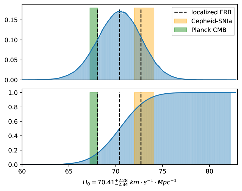
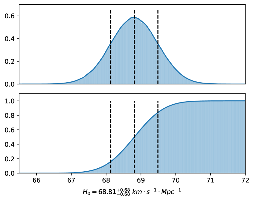
The histogram of all samples is plotted with bin-width chosen according to Freedman Diaconis rule implemented by numpy, and the probability density function (PDF) is given by kernel density estimation (KDE). We also plot cumulative histogram to get the cumulative distribution function (CDF), and the confidence interval is as shown in Fig. 1. Our constraint from localized FRBs lies between early-time result given by Planck Collaboration et al. (2020) and late-time result given by Riess et al. (2022), which supports that FRBs can be used as individual cosmological probes to constrain .
4 Constraint with unlocalized FRBs
Though the number of localized FRBs is increasing rapidly, an absolute majority still remain unlocalized, therefore it is crucial to utilize unlocalized FRBs. A common solution is to inverse "pseudo redshifts" with observed DM (Tang et al., 2023). Compared with another method of simply generating FRB data with simulation, FRBs with pseudo redshift are not dependent on any pre-assumption of DM distribution, and use real DM data as its foundation. We collect data of unlocalized FRBs from CHIME database. We used all bursts in CHIME catalog 1 (CHIME/FRB Collaboration et al., 2021) and part of available repetitive bursts with definite coordinates in CHIME catalog 2023 (Chime/Frb Collaboration et al., 2023) to run MCMC simulation. Note that when processing repetitive FRBs, we consider all bursts from the same source as one single event, and calculate their mean DM as . With pseudo redshifts, we could utilize all unlocalized FRBs as localized ones to constrain Hubble constant.
4.1 Pseudo redshift
4.1.1 Circular argument
Before estimating pseudo redshifts, a pre-determined value for is required, which may lead to a "circular argument" by assuming to be a certain value while calculating . However it can be considered as an iterative analysis similar to Newton-Raphson method, where we assume an initial value to calculate pseudo redshift , and apply to estimate . To be precise, this step should repeat as
| (12) |
until . Yet we find that the difference of initial value for has little influence on pseudo redshift and therefore even less influence on final estimation of , and our initial value is actually close enough with final result (), thus we skip the latter parts in Equation (12).
Another way to avoid circular argument is to consider as an unfitted parameter same as pseudo redshift instead of pre-assuming its value. To guarantee that the fit is the same for all FRBs, it is required to calculate pseudo redshift for all FRBs at the same time, i.e. to fit simultaneously. For , an enormous computational resource is required to fit a 528-dimensional parameter space. In comparison, we could run 527 individual simulations using Equation (12), and fit pseudo redshift for each FRB at a time, which can significantly reduce computation.
4.1.2 Calculating pseudo redshifts
To estimate pseudo redshifts, there are two different methods: maximum likelihood estimation and Monte Carlo simulation. Both methods require a likelihood function slightly different from Equation 9. is now a known parameter while is the unfitted variable. The equation is rewrote as:
| (13) | ||||
MLE can give the mean value of pseudo redshift for each FRB, yet the chain may fail to converge for FRBs with extremely low dispersion measure ( ), and MLE gives no information about its distribution. Monte Carlo simulation provides probability density distribution and works for FRBs with low DM.
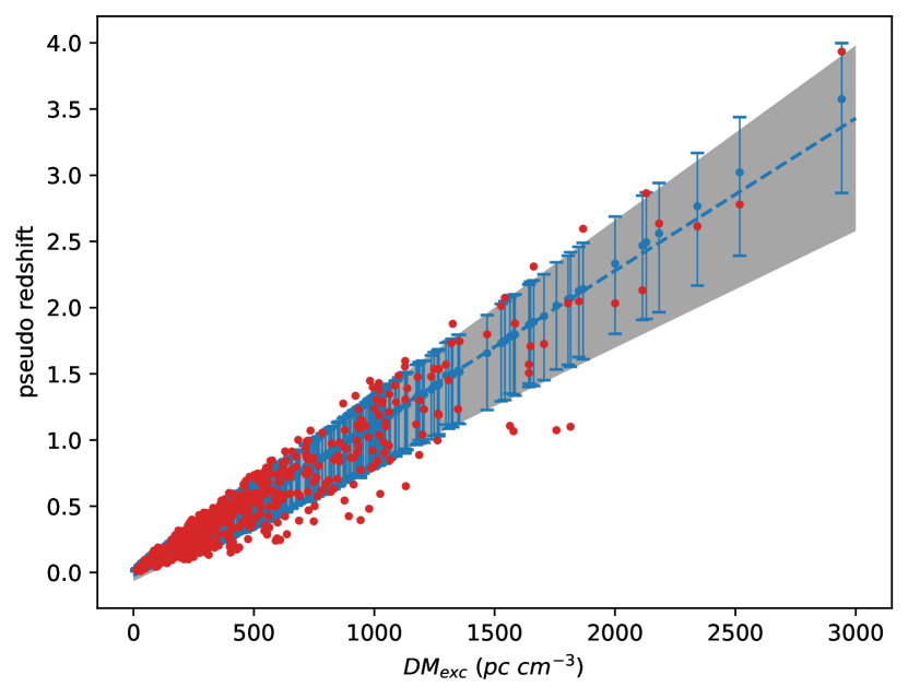
With similar MCMC simulation as described in Section 3.2.2, 57600 samples (=64, discard=100, steps=1000) are generated for each single FRB. We calculate the 16, 50, 84 percentile of pseudo redshift for each FRB and plot them in the form of errorbar on a scatterplot with dispersion measure as horizontal axis. For any given percentile ( or for example), shows a good linear relation, which agrees with pseudo redshift result in previous researches. We plot result of linear regression and show the 68% confidence region in Fig. 2.
4.2 PDF of pseudo redshifts
4.2.1 Fitting with Gaussian-like distribution function
To apply pseudo redshifts in estimating , probability density distribution of pseudo redshift for each FRB is required. One simplest way to fit is to use a Gaussian distribution. However, an ordinary Gaussian distribution is symmetric while our samples are not necessarily symmetric. Also, Gaussian function extends to infinity in both directions, for example, we have and , which obviously does not make sense in physical reality. To adapt Gaussian distribution to our usage, we must truncate Gaussian distribution.
There is an existing distribution called truncated normal distribution, which is a Gaussian-like function where variable is limited within a given region. It is implemented with such method: sample with an ordinary Gaussian distribution, and resample if the variable is out of boundary. It is easy to prove that this method does not change relative proportions of probability within allowed region, thus a truncated normal distribution is same as a cut-off Gaussian distribution which is "stretched" for normalization, and their PDF writes as:
| (14) |
where and are PDF and CDF of standard Gaussian distribution. With limitation parameters and , we can now introduce the asymmetry of original KDE into truncated normal distribution.
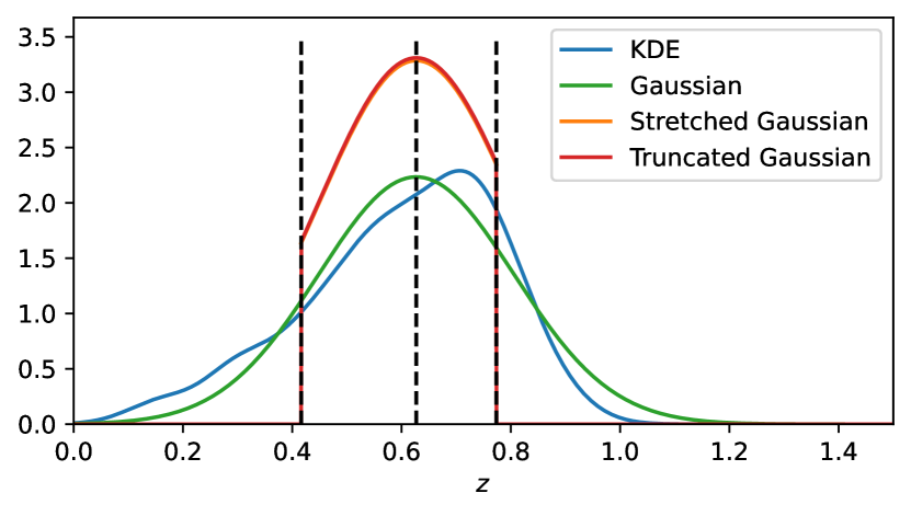
Taking FRB20180725A as an example, we plot Gaussian distribution and truncated normal distribution (limited within interval) in Fig. 3. Parameters for Gaussian distribution is , and parameters for truncated normal distribution is where and are percentiles of pseudo redshifts. However, truncated normal distribution does not work well in MCMC simulation. The chain fails to converge after a long time of simulation. One possible reason is that the truncated function is too "flat" within region, and the difference is diluted. As shown in Fig. 3, the probability density around is fairly high and its difference from peak probability is insignificant.
4.2.2 Sampling directly from MCMC results
In fact, the best way to describe pseudo redshift is using the KDE function, yet there is no analytic expression. Instead of looking for a probability function to fit the KDE as Section 4.2.1 does, sampling directly from MCMC results is a more accurate yet more computational-costing way. For each FRB, the 57600 samples generated in Section 4.1 naturally follow the PDF of pseudo redshift, and randomly sampling from them will provide a statistical variable following the same PDF. Since such method requires much computation, we thin the samples with a ratio of 1:50 to greatly reduce the computation and also to avoid small-probability values. Our tests show that sampling among 1152 thinned samples gives results with little difference from original KDE function.
4.3 Simulation of unlocalized FRBs
With all data of pseudo redshifts for unlocalized FRBs prepared, difference still exists between simulation of localized and unlocalized FRBs. Generally there are two methods of simulating: integrating with entire probability density, and using randomly scattered pseudo redshifts, both of which are necessary to give a comprehensive understanding of constraint on Hubble constant.
4.3.1 Using integral of probability distribution
To get a more precise result on the estimated value of , the best way is to integrate pseudo redshifts within MCMC simulation. This will add another level of integral in Equation (9), which becomes:
| (15) | ||||
where is normalized PDF of pseudo redshift. Obviously Equation (15) would significantly increase computation. An alternative method is to randomly pick one value for following its PDF within each MCMC step. With steps for each FRB, it is reasonable to believe such sampling can well reflect probability distribution of pseudo redshifts. This greatly reduces computation compared with the former method, yet the values of redshift keep changing within a considerable range for each MCMC step, which makes the chain extremely hard to converge.
To avoid constant fluctuation of redshifts, we use median values of pseudo redshifts (blue dots in Fig. 2) in simulation. Median values indicate the expectation of probability distribution, and do not cause unacceptable computation or divergence of the chain.
4.3.2 Using randomly scattered pseudo redshifts
Despite the expectation of the probability distribution providing the most possible median value of that we would find if all FRBs were localized, it does not tell us about the uncertainty of the constraint. Assume that all FRBs have been localized and we try to constrain with their redshifts under these given circumstances:
(a) the redshifts are found to be exactly the median values of our simulation (blue dots in Fig. 2);
(b) the redshifts are found to randomly scatter around the median values following the probability distribution (red dots in Fig. 2).
The uncertainty of given by our hypothetical constraint under both conditions could be different. To be precise, (b) is most likely to give a constraint less tight than (a), thus results from Section 4.3.1 is not enough to predict the comprehensive result of constraint with unlocalized FRBs.
To simulate a condition described in (b), which is also more likely to actually happen than in (a), we assign a fixed value of redshift for each FRB by randomly scattering values following the PDF of pseudo redshifts around the median value. After discussions in Section 4.2, we directly sample from MCMC simulation samples to get a value which follows the PDF instead of fitting the KDE function. By sampling "around the median value", we mean that extreme samples (below 3% or above 97%) from MCMC simulation are discarded, and we only sample from the rest 94% interval. The scattered values are shown as red dots in Fig. 2.
4.3.3 Results of unlocalized FRBs
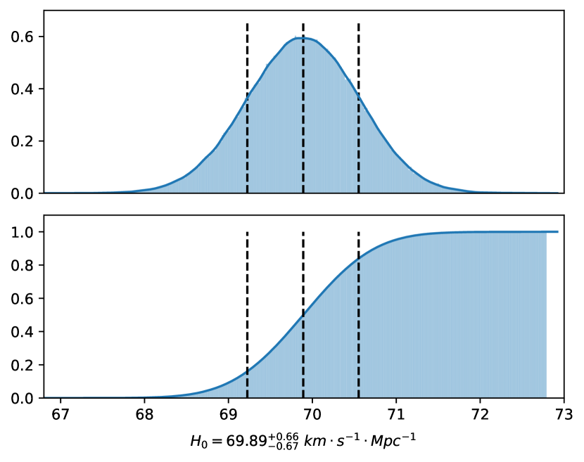
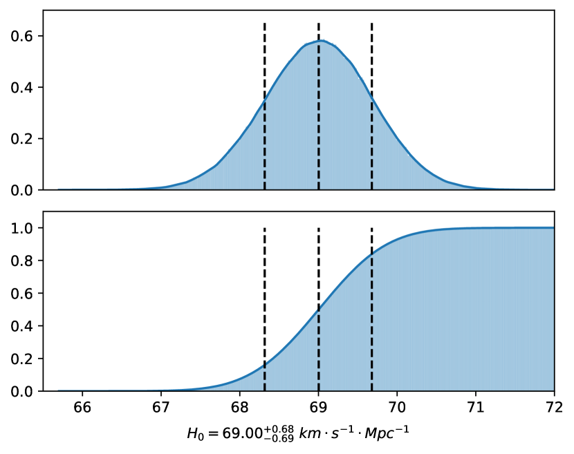
We run MCMC simulation in a way most similar to Section 3 with different pseudo redshift values as described in Sections 4.3.1 and 4.3.2. Simulation with median redshifts gives a 68% confidence interval of as shown in Fig. 4. Simulation with scattered redshifts gives as shown in Fig. 5. The results differ slightly in expectation of , yet show little difference in uncertainty.
The median value seems to deviate from the median value constrained with localized FRBs, yet still lies in the confidence interval in Fig. 1. In comparison, since the redshifts are "pseudo", the uncertainty of result from unlocalized FRBs is much more inspiring than the median value. It provides a convincing prediction that if all 527 FRBs are localized, the uncertainty will drop to at confidence. Compared with result of localized FRBs, we have and . The ratios slightly deviate from the relation . A possible explanation is that the number of localized FRBs is still limited, and the real redshift distribution does not exactly follow the relation we simulated.
5 Discussion
By introducing 527 unlocalized CHIME FRBs and using scattered pseudo redshifts, the uncertainty of constraint is significantly reduced. However, some bias and error must be included for a full discussion. We generally divide them into statistical error and systematic error.
5.1 Statistical error
Statistical error mainly refers to the error of cosmological parameters and appeared in Equation (5). The error of will be discussed in Section 5.2, and other constant in Equation (5) such as and are already measured with extremely high precision. Planck Collaboration et al. (2020) gave and .
For , it appears in Equation (5) as a linear term. Assuming a Gaussian distribution around , we can do a rough estimation:
| (16) |
which shows a symmetric distribution of has little influence on . Furthermore, the precision of () is slightly smaller than that of of our constraint ().
For , which appears inside the integral in Equation (5), it has an uncertainty of and could not be ignored. To marginalize , the best way is to add another level of integral, which would significantly increase computation. Alternatively, we consider replacing integral with expansion. Assume a Gaussian distribution with , , the integral can be wrote as:
| (17) | ||||
where is the normalization factor and is our target function. Note that is redshift of FRB, and is our integration variable. Since both and could not be expressed by elementary functions, we perform a series expansion on around and get . We plot the figure of at different and compare it with original function to ensure the expansion is acceptable. Now the inner integral in Equation (17) can be wrote as an explicit function of , i.e. . However, the form of is still too complicated to integrate, thus we need to do another series expansion around . To determine the best value for , we plot the expanded function at different and degrees. It is found that expanding to the term of around provides best fit for both and . Denote it as , and we can complete the whole integral: .
Taking the new expression into Equation (5), we could run MCMC simulation with marginalized. The result is shown in Fig. 6 (we use the method in Section 4.3.2). The confidence interval of is and has little difference with previous result in Fig. 5, which indicates that the statistical error of does not influence constraint on significantly.
5.2 Systematic errors
There are several systematic errors that need to be discussed. In Equation (5), compared with and , the fraction of baryon in IGM may introduce more uncertainty. However, we still know little about . Shull et al. (2012) gave the value of yet does not propose the errorbar. Connor et al. (2024) provided a more accurate constraint, yet it depends on several other models and theories. Furthermore, it is difficult for any constraint using Equation (5) to separate the error of from as they appear in a coupling term in Equation (5). To be precise, only constraint on can be made instead of constraint on . So, the value of must be determined by other approaches when constraining from FRBs. By fixing , it has been found that the uncertainty of is about 8% (Yang et al., 2022; Connor et al., 2024). Obviously, the systematic error from dominates the error of measured at present. On the other hand, it may varies with redshift. Researches with other methods are needed to further investigate the error of .
includes all contributions to DM that come from FRB host galaxy. Using IllustrisTNG simulations, the probabilty distribution of including the local cosmic structure (e.g. filament) halo and interstellar medium of the host have been derived (Zhang et al., 2020). However, the vicinity environment of FRB progenitors have not been considered. The most promising progenitors of FRBs are young magnetars, which can be formed by core-collapse of massive stars or mergers of two compact objects (Wang et al., 2020). So they may be embedded in a magnetar wind nebula and supernova remnant (Yang & Zhang, 2017; Piro & Gaensler, 2018; Zhao & Wang, 2021). Meanwhile, the largest with rotation measure reversal for FRB 20190520B indicates it may reside in a binary system (Wang et al., 2022; Anna-Thomas et al., 2023). So similar FRBs should be removed when measuring . For FRBs with little DM contribution from vicinity environment, precise modelling should be performed. It is important to use optical observations of the FRB host galaxy environment, combined with the rotation measure and scattering times of FRBs to constrain (Cordes et al., 2022).
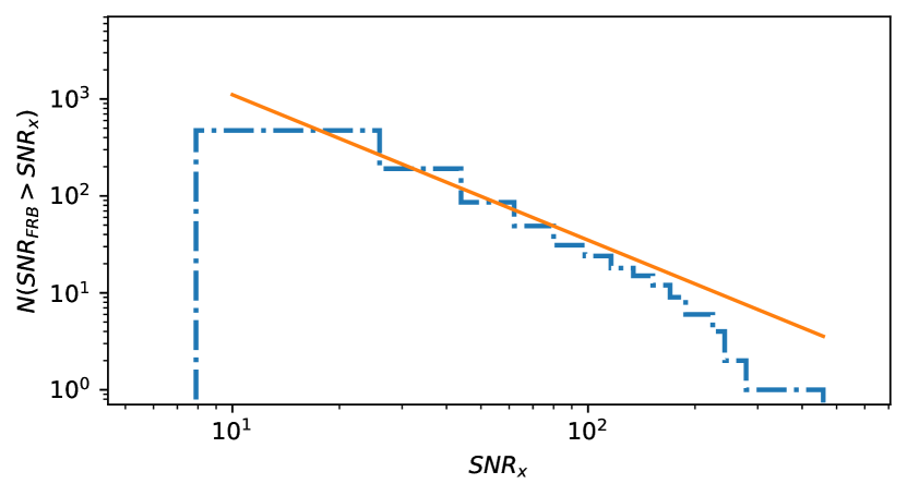
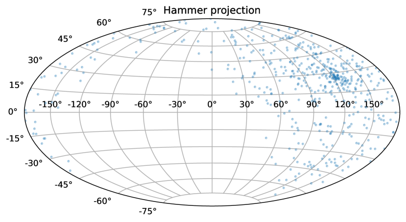
Several selection biases should be discussed, such as SNR effect, ISM effect, selection effect of unlocalized FRBs and gridding effect (James et al., 2022). For the latter two effects, our constraint has no such error since we make use of most unlocalized FRBs in CHIME database and use continuous value for redshift and dispersion measures instead of discrete variables. For SNR effect, the log-log figure of number of events observed above SNR threshold should follow power law of -1.5 (in log-log plot, i.e. ), and James et al. (2022) found that events from CRAFT/ICS deviates from the -1.5 power law. We plot the same figure with unlocalized FRBs from CHIME database in Fig. 7, and the histogram followed the power law well, thus our constraint is not much influenced by SNR effect. Finally, for the ISM effect, James et al. (2022) claimed that would increase at low galactic latitude, which may prevent telescopes from observing such events. We plot Hammer projection of FRBs in galactic coordinate system in Fig. 8. Hammer projection is an equal-area projection and there are a considerable amount of FRBs located in low galactic latitude area. Furthermore, few of these low-galactic-latitude FRBs have shown extreme values of even above 200. Thus ISM effect could be ignored during our constraint using unlocalized FRBs.
6 Conclusions
We run MCMC simulations to constrain Hubble constant using 69 localized FRBs and 527 unlocalized FRBs from CHIME catalog respectively. We apply redshift-dispersion measure relation and Bayesian estimation to build MCMC model. We use normalization factors obtained from IllustrisTNG simulation to model DM distribution. For localized FRBs, we get the result of with 69 FRBs, which lies between constraints from late-time and early-time research, further proving FRB to be an individual cosmological probe. For unlocalized FRBs, we run individual MCMC simulation instead of maximum likelihood estimation to get probability density distribution of pseudo redshift for each FRB. We use direct sampling instead of fitting kernel density estimation function to draw samples of pseudo redshifts. We combine two different methods of using pseudo redshifts to get a comprehensive constraint on Hubble constant, i.e. to use median value of redshifts and to use fixed scattered redshifts, which gives the result of and respectively.
We discuss statistical errors of cosmological parameters and systematic errors of and selection biases. We show that the statistical error of has a minor influence on our constraint compared to , and we perform a series expansion to marginalize and obtain the result of . We find that the coupling effect prevents us from separate the error of from . The uncertainty of is dominated by the error of the fraction of cosmic baryons in diffuse ionized gas . Other systematic errors could be neglected.
Our study gives a prediction of future constraint on Hubble constant with more localized FRBs. Our result shows that the uncertainty of Hubble constant is likely to drop to if the number of localized FRBs is raised to . We believe that with more samples localized, FRBs will become a powerful individual tool to solve Hubble Tension.
Acknowledgements
This work was supported by the National Natural Science Foundation of China (grant No. 12273009), the National SKA Program of China (grant No. 2022SKA0130100), the China Manned Spaced Project (CMS-CSST-2021-A12) and the Natural Science Foundation of Xinjiang Uygur Autonomous Region (grant No. 2023D01E20).
Data Availability
The data used is shown in Table 1 and relevant references.
References
- Anna-Thomas et al. (2023) Anna-Thomas R., et al., 2023, Science, 380, 599
- Bannister et al. (2019) Bannister K. W., et al., 2019, Science, 365, 565
- Bhandari & Flynn (2021) Bhandari S., Flynn C., 2021, Universe, 7
- Bhandari et al. (2020) Bhandari S., et al., 2020, ApJ, 895, L37
- Bhandari et al. (2022) Bhandari S., et al., 2022, AJ, 163, 69
- Bhandari et al. (2023) Bhandari S., et al., 2023, ApJ, 948, 67
- Bhardwaj et al. (2021) Bhardwaj M., et al., 2021, ApJ, 919, L24
- Bhattacharya et al. (2021) Bhattacharya M., Kumar P., Linder E. V., 2021, Physical Review D, 103, 103526
- CHIME/FRB Collaboration et al. (2021) CHIME/FRB Collaboration et al., 2021, ApJS, 257, 59
- Caleb et al. (2023) Caleb M., et al., 2023, MNRAS, 524, 2064
- Cassanelli et al. (2023) Cassanelli T., et al., 2023, A fast radio burst localized at detection to a galactic disk using very long baseline interferometry (arXiv:2307.09502)
- Chatterjee et al. (2017) Chatterjee S., et al., 2017, Nature, 541, 58
- Chime/Frb Collaboration et al. (2023) Chime/Frb Collaboration et al., 2023, ApJ, 947, 83
- Chittidi et al. (2021) Chittidi J. S., et al., 2021, ApJ, 922, 173
- Connor et al. (2024) Connor L., et al., 2024, A gas rich cosmic web revealed by partitioning the missing baryons (arXiv:2409.16952), https://arxiv.org/abs/2409.16952
- Cooke et al. (2018) Cooke R. J., Pettini M., Steidel C. C., 2018, ApJ, 855, 102
- Cordes & Chatterjee (2019) Cordes J. M., Chatterjee S., 2019, Annual Review of Astronomy and Astrophysics, 57, 417
- Cordes & Lazio (2002) Cordes J. M., Lazio T. J. W., 2002, arXiv e-prints, pp astro–ph/0207156
- Cordes et al. (2022) Cordes J. M., Ocker S. K., Chatterjee S., 2022, ApJ, 931, 88
- Deng & Zhang (2014) Deng W., Zhang B., 2014, ApJ, 783, L35
- Driessen et al. (2023) Driessen L. N., et al., 2023, MNRAS, 527, 3659
- Freedman (2021) Freedman W. L., 2021, ApJ, 919, 16
- Gao et al. (2024) Gao J., Zhou Z., Du M., Zou R., Hu J., Xu L., 2024, MNRAS, 527, 7861
- Goodman & Weare (2010) Goodman J., Weare J., 2010, Communications in Applied Mathematics and Computational Science, 5, 65
- Gordon et al. (2023) Gordon A. C., et al., 2023, The Demographics, Stellar Populations, and Star Formation Histories of Fast Radio Burst Host Galaxies: Implications for the Progenitors (arXiv:2302.05465), https://arxiv.org/abs/2302.05465
- Hagstotz et al. (2022) Hagstotz S., Reischke R., Lilow R., 2022, MNRAS, 511, 662
- Heintz et al. (2020) Heintz K. E., et al., 2020, ApJ, 903, 152
- Hu & Wang (2023) Hu J.-P., Wang F.-Y., 2023, Universe, 9, 94
- Hubble (1929) Hubble E., 1929, Proceedings of the National Academy of Science, 15, 168
- James et al. (2022) James C. W., et al., 2022, MNRAS, 516, 4862
- Kalita et al. (2024) Kalita S., Bhatporia S., Weltman A., 2024, Fast Radio Bursts as probes of the late-time universe: a new insight on the Hubble tension (arXiv:2410.01974), https://arxiv.org/abs/2410.01974
- Keane et al. (2012) Keane E. F., Stappers B. W., Kramer M., Lyne A. G., 2012, MNRAS, 425, L71
- Kirsten et al. (2022) Kirsten F., et al., 2022, Nature, 602
- Kumar & Linder (2019) Kumar P., Linder E. V., 2019, Physical Review D, 100, 083533
- Law et al. (2020) Law C. J., et al., 2020, ApJ, 899, 161
- Law et al. (2024) Law C. J., et al., 2024, Deep Synoptic Array Science: First FRB and Host Galaxy Catalog (arXiv:2307.03344)
- Li et al. (2020) Li Z., Gao H., Wei J. J., Yang Y. P., Zhang B., Zhu Z. H., 2020, MNRAS, 496, L28
- Lin & Zou (2023) Lin H.-N., Zou R., 2023, Monthly Notices of the Royal Astronomical Society, 520, 6237
- Lin et al. (2023) Lin H.-N., Tang L., Zou R., 2023, Monthly Notices of the Royal Astronomical Society, 520, 1324
- Lorimer et al. (2007) Lorimer D. R., Bailes M., McLaughlin M. A., Narkevic D. J., Crawford F., 2007, Science, 318, 777
- Macquart et al. (2020a) Macquart J. P., et al., 2020a, Nature, 581, 391
- Macquart et al. (2020b) Macquart J. P., et al., 2020b, Nature, 581, 391
- Mahony et al. (2018) Mahony E. K., et al., 2018, The Astrophysical Journal Letters, 867, L10
- Marcote et al. (2020) Marcote B., et al., 2020, Nature, 577, 190
- McQuinn (2013) McQuinn M., 2013, ApJ, 780, L33
- Michilli et al. (2023) Michilli D., et al., 2023, ApJ, 950, 134
- Muñoz et al. (2016) Muñoz J. B., Kovetz E. D., Dai L., Kamionkowski M., 2016, Physical Review Letters, 117, 091301
- Niu et al. (2022) Niu C.-H., et al., 2022, Nature, 606, 873
- Ocker et al. (2021) Ocker S. K., Cordes J. M., Chatterjee S., 2021, ApJ, 911, 102
- Petroff et al. (2022) Petroff E., Hessels J. W. T., Lorimer D. R., 2022, A&ARv, 30, 2
- Pillepich et al. (2017) Pillepich A., et al., 2017, MNRAS, 473, 4077
- Piro & Gaensler (2018) Piro A. L., Gaensler B. M., 2018, ApJ, 861, 150
- Planck Collaboration et al. (2020) Planck Collaboration et al., 2020, A&A, 641, A6
- Prochaska & Zheng (2019) Prochaska J. X., Zheng Y., 2019, MNRAS, 485, 648
- Prochaska et al. (2019) Prochaska J. X., et al., 2019, Science, 366, 231
- Qiu et al. (2022) Qiu X.-W., Zhao Z.-W., Wang L.-F., Zhang J.-F., Zhang X., 2022, Journal of Cosmology and Astroparticle Physics, 2022, 006
- Rajwade et al. (2022) Rajwade K. M., et al., 2022, Monthly Notices of the Royal Astronomical Society, 514, 1961–1974
- Ravi et al. (2019) Ravi V., et al., 2019, Nature, 572, 352
- Ravi et al. (2022) Ravi V., et al., 2022, MNRAS, 513, 982
- Ravi et al. (2023a) Ravi V., et al., 2023a, Deep Synoptic Array science: a 50 Mpc fast radio burst constrains the mass of the Milky Way circumgalactic medium (arXiv:2301.01000)
- Ravi et al. (2023b) Ravi V., et al., 2023b, ApJ, 949, L3
- Riess et al. (2022) Riess A. G., et al., 2022, ApJ, 934, L7
- Ryder et al. (2023) Ryder S. D., et al., 2023, Science, 382, 294
- Sharma et al. (2024) Sharma K., et al., 2024, Preferential Occurrence of Fast Radio Bursts in Massive Star-Forming Galaxies (arXiv:2409.16964), https://arxiv.org/abs/2409.16964
- Shull et al. (2012) Shull J. M., Smith B. D., Danforth C. W., 2012, ApJ, 759, 23
- Tang et al. (2023) Tang L., Lin H.-N., Li X., 2023, Chinese Physics C, 47, 085105
- Tendulkar et al. (2017) Tendulkar S. P., et al., 2017, ApJ, 834, L7
- Thornton et al. (2013) Thornton D., et al., 2013, Science, 341, 53
- Valentino et al. (2021) Valentino E. D., et al., 2021, Classical and Quantum Gravity, 38, 153001
- Walters et al. (2018) Walters A., Weltman A., Gaensler B. M., Ma Y.-Z., Witzemann A., 2018, ApJ, 856, 65
- Wang & Wang (2018) Wang Y. K., Wang F. Y., 2018, Astronomy & Astrophysics, 614, A50
- Wang & Wei (2023) Wang B., Wei J.-J., 2023, ApJ, 944, 50
- Wang et al. (2020) Wang F. Y., Wang Y. Y., Yang Y.-P., Yu Y. W., Zuo Z. Y., Dai Z. G., 2020, ApJ, 891, 72
- Wang et al. (2021) Wang H., Miao X., Shao L., 2021, Physics Letters B, 820, 136596
- Wang et al. (2022) Wang F. Y., Zhang G. Q., Dai Z. G., Cheng K. S., 2022, Nature Communications, 13, 4382
- Wang et al. (2024) Wang Y.-B., Zhou X., Kurban A., Wang F.-Y., 2024, ApJ, 965, 38
- Wei & Melia (2023) Wei J.-J., Melia F., 2023, ApJ, 955, 101
- Wu & Wang (2024) Wu Q., Wang F.-Y., 2024, arXiv e-prints, p. arXiv:2409.13247
- Wu et al. (2020) Wu Q., Yu H., Wang F. Y., 2020, ApJ, 895, 33
- Wu et al. (2022) Wu Q., Zhang G.-Q., Wang F.-Y., 2022, MNRAS, 515, L1
- Xiao et al. (2021) Xiao D., Wang F., Dai Z., 2021, Science China Physics, Mechanics, and Astronomy, 64, 249501
- Yang & Zhang (2017) Yang Y.-P., Zhang B., 2017, ApJ, 847, 22
- Yang et al. (2022) Yang K. B., Wu Q., Wang F. Y., 2022, ApJ, 940, L29
- Yao et al. (2017) Yao J. M., Manchester R. N., Wang N., 2017, ApJ, 835, 29
- Zhang (2023) Zhang B., 2023, Reviews of Modern Physics, 95, 035005
- Zhang et al. (2020) Zhang G. Q., Yu H., He J. H., Wang F. Y., 2020, ApJ, 900, 170
- Zhang et al. (2021) Zhang Z. J., Yan K., Li C. M., Zhang G. Q., Wang F. Y., 2021, ApJ, 906, 49
- Zhao & Wang (2021) Zhao Z. Y., Wang F. Y., 2021, ApJ, 923, L17
- Zhao et al. (2022) Zhao Z.-W., Zhang J.-G., Li Y., Zhang J.-F., Zhang X., 2022, arXiv e-prints, p. arXiv:2212.13433
- Zhou et al. (2014) Zhou B., Li X., Wang T., Fan Y.-Z., Wei D.-M., 2014, Physical Review D, 89, 107303