Mechanics of metric frustration in contorted filament bundles:
From local symmetry to columnar elasticity

Elastic zero modes are a ubiquitous feature of soft materials, from mechanical metamaterials [1, 2] to liquid crystal elastomers [3]. Such systems can undergo large deformations with minimal strain, as geometrically coupled rotations and translations preserve local spacing between microscopic constituents. The smectic and columnar liquid crystalline phases provide paradigmatic examples of zero modes in soft elastic systems, permitting relative “sliding” of 2D layers and 1D columns, respectively. The zero-cost sliding displacements of smectic and columnar phases are characteristic of a much broader class of laminated and filamentous structures, ranging from multi-layer graphene materials [4] and stacked paper [5] to biopolymer bundles [6, 7], nanotube yarns [8], wire ropes [9].

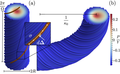
While there are well established frameworks which capture the geometric nonlinearities of smectic liquid crystals (i.e., the strain tensor accurately describes arbitrarily large and complex deformations) [10], no such framework exists for columnar and filamentous materials. The orientations of column backbones impose constraints on inter-filament spacing, generating rich modes of geometric frustration without counterpart in smectic liquid crystals. In the simplest non-trivial case of helical bundles, predictions from a minimally non-linear approximation of columnar elasticity [11] and tomographic analysis of elastic filament bundles [12] show that twist in straight bundles gives rise to non-uniform inter-filament stress and spacing in transverse sections (see Fig 1a). Except for the restrictive classes of straight, twisted bundles [13] and twist-free developable domains [14, 15], bundle textures also generate longitudinal frustration, requiring local spacings to vary along a bundle [16]. Although deformations that introduce longitudinal frustration are the rule rather than the exception—for example, wire ropes or toroidal biopolymer condensates are both twisted and bent (e.g. Fig. 1)—existing frameworks of columnar elasticity fail to capture this effect.

In this Letter, we develop a fully geometrically non-linear Lagrangian elasticity theory of columnar materials, which completely captures the interplay between orientation, and both lateral and longitudinal frustration of inter-filament spacing. We construct this theory by imposing a gauge-like local symmetry under reptations, deformations that slide filaments along their contours without changing the inter-filament spacing. The resultant equilibrium equations point to the role geometrical measures of non-equidistance play in bundles’ mechanics. Within this framework, we compute the energetic costs of longitudinal frustration in twisted, toroidal bundles, and give evidence that 1) optimal configurations generically incorporate splay and 2) the bending cost that derives from non-uniform compression depends non-monotonically on pretwist.

To construct the elastic theory, we divide space into points on curves (i.e. filament backbones) labeled by two coordinates: $\mathbf{v}$, a 2D label of filaments; and $s$, a length coordinate along filaments. Hence, the location of each point in the bundle is described by a function $\mathbf{r}(s,\mathbf{v})$, with $\partial_{s}\mathbf{r}(s,\mathbf{v})$ parallel to the tangent vector $\mathbf{t}={\partial_{s}\mathbf{r}}/{|\partial_{s}\mathbf{r}|}$. Because they lack positional order along their backbone curves, filament bundles and columnar liquid crystals have a family of continuous zero modes, corresponding to reptations (Fig. 1),

We assume that changes in local spacing can be described by a hyper-elastic energy density function ${\cal W}$, that depends only on the deformation gradient [17].

To account for reptation symmetry, we demand that ${\cal W}$ depend on a modified deformation gradient, which transforms as a scalar under $\sigma(s,\mathbf{v})$, depends solely on the deformation, $\mathbf{r}$, of the material itself, and recovers the well-established 2D elasticity of developable [14, 15] bundles. Specifically, we construct a covariant derivative $D_{I}\mathbf{r}=\nabla_{I}\mathbf{r}-\mathbf{A}_{I}$, where $\nabla_{I}$ is the usual covariant derivative on tensors in the material space and $\mathbf{r}$ determines $\mathbf{A}_{I}$, such that if two configurations, $\mathbf{r}$ and $\mathbf{r}^{\prime}$, are related by Eq. (1), then $D_{I}\mathbf{r}=D^{\prime}_{I}\mathbf{r}^{\prime}$. In order for $D_{I}\mathbf{r}$ to be reptation invariant, we must have that $-\mathbf{A}^{\prime}_{I}+\mathbf{A}_{I}=\nabla_{I}\sigma\partial_{s}\mathbf{r}$. Therefore, $-\mathbf{A}^{\prime}_{I}+\mathbf{A}_{I}=-(\mathbf{t}\cdot\nabla_{I}\mathbf{r}^{\prime})\mathbf{t}+(\mathbf{t}\cdot\nabla_{I}\mathbf{r})\mathbf{t}$. To construct an elastic theory of columnar materials, we set $\mathbf{A}_{I}=(\mathbf{t}\cdot\nabla_{I}\mathbf{r})\mathbf{t}$, which is manifestly reptation invariant but also leads to a deformation gradient that only measures deformations transverse to the local backbones,

Notably, for two nearby filaments at ${\bf r}({\bf v})$ and ${\bf r}({\bf v}+d{\bf v})$ in material coordinates, it is straightforward to show that the covariant derivative gives the local distance of closest approach $d{\bf\Delta}=dv^{I}~{}D_{I}\mathbf{r}$, for which $d{\bf\Delta}\cdot{\bf t}=0$ (see again inset of Fig. 1a). As shown explicitly in the Appendix, this covariant deformation gradient captures the standard 2D deformation gradients of developable domains (i.e. parallel arrays).

From this deformation gradient, we construct an effective metric $g^{\text{eff}}_{IJ}=D_{I}\mathbf{r}\cdot D_{J}\mathbf{r}$, which is naturally invariant under rotations of $\mathbf{r}$, and which encodes the metric inherited by the local 2D section transverse to the filaments in the bundle ¹¹1Equidistant bundles where components of $g^{\text{eff}}_{IJ}$ are uniform along $s$ are known as Riemannian fibrations, see e.g.  [36, 37], and the transverse structure can be mapped on to single 2D base space. Non-equidistant bundles correspond to Sub-Riemannian generalizations [38] where the inherited metric measures distances in the 2-planes perpendicular to ${\bf t}$ at each point.. Because $D_{s}\mathbf{r}=0$, the effective metric only has components for $2\times 2$ block $I,J\neq s$, which we denote using index notation $\alpha$, $\beta\in\{1,2\}$. With these definitions, we construct the Green-Saint-Venant strain tensor, [17, 19, 20]

where $g_{\alpha\beta}^{\text{tar}}$ is the target metric corresponding to strain-free state, which for this Letter, we take to be developable with uniform spacing, so $g_{\alpha\beta}^{\text{tar}}=\delta_{\alpha\beta}$. For weak deflections from the uniform parallel state, Eq. (3) reduces to the small-tilt approximation to the non-linear columnar strain [21, 22, 11], which captures the lowest-order dependence of spacing on orientation (see Appendix).

Assuming that strains are small though deformations may be large, the Hookean elastic energy takes the usual form,

where $S^{\alpha\beta}=\tfrac{\partial{\cal W}}{\partial\epsilon_{\alpha\beta}}=C^{\alpha\beta\gamma\delta}\epsilon_{\gamma\delta}$ is the nominal stress tensor, and $C^{\alpha\beta\gamma\delta}$ is a tensor of elastic constants which depends on both the crystalline symmetries of the underlying columnar order and the target metric, $g_{\alpha\beta}^{\text{tar}}$ ²²2We raise and lower indices with $g^{\alpha\beta\text{tar}}$, the inverse of $g_{\alpha\beta}^{\text{tar}}$, rather than $g^{\alpha\beta\text{eff}}$, as a matter of convenience, and note that the difference in the elastic energy is higher order in the strain tensor [20].. Energetics of columnar materials also include other gauge-invariant costs, including the Frank-Oseen orientational free energy and the cost of local density changes along columns ³³3The symmetry under local reptations in this theory is unlike a related treatment of both the nematic to smectic-A transition [39, 40] and its columnar analog [41, 42, 43] in which the gauge symmetry of a density-wave is explicitly broken by, e.g., the splay elasticity of the underlying nematic order.. Here, for clarity, we focus only on the energetics of columnar strain and detail the combined effects of other contributions elsewhere [25]. Given this gauge-invariant formulation of the columnar strain energy, we first illustrate the mechanical effects of orientational geometry on local forces. This follows from the bulk Euler-Lagrange equations of Eq. (21) (see Appendix for a complete derivation),

The bulk terms represent body forces generated by the columnar strains, which must be balanced by other internal stresses or external forces. To cast them in a more geometrical light, we consider separately the components tangential and perpendicular to ${\bf t}$, $F_{\parallel}$ and ${\bf F}_{\perp}$, respectively.

Making use of the identity, ${\bf t}\cdot\nabla_{\alpha}D_{\beta}{\bf r}=-\partial_{\alpha}{\bf t}\cdot\partial_{\beta}{\bf r}$, the tangential forces can be recast simply as

where

is the convective flow tensor that measures longitudinal variations in inter-filament spacing [16]. Just as the second fundamental form measures gradients of a surface’s normal vector [26], $h_{\alpha\beta}$ measure the symmetric gradients of $\mathbf{t}$ in its normal plane (i.e. its trace is the splay of filament tangents).

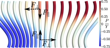
Here, we see that tangent forces couple non-equidistance to the stress tensor much like the Young-Laplace law couples in-plane stresses to normal forces in curved membranes [19]. This analogy becomes exact for zero twist textures: when $\mathbf{t}\cdot(\nabla\times\mathbf{t})=0$, filaments can be described by a set of surfaces normal to $\mathbf{t}$. In this case, it is possible to choose coordinates so that $\partial_{\alpha}{\bf r}\cdot{\bf t}=0$, and tangential forces give the Young-Laplace force normal to each surface, with $h_{\alpha\beta}$ reducing to their second fundamental form. This illustrates the intuitive notion, shown schematically in Fig. 2, that columnar strain generates tangential body forces that push material points towards lower-stress locations in the array.

The bulk components of Eq. (30) perpendicular to $\mathbf{t}$ give the transverse force

This form captures the divergence of stress in the planes perpendicular to backbones. The second term accounts for the corrections arising from material derivatives that lie along the backbone, such as twisted textures, when $\partial_{\alpha}{\bf r}\cdot{\bf t}\neq 0$. Thus, the longitudinal derivatives in $\mathbf{F}_{\perp}$ are needed to capture transverse mechanics of even equidistant twisted bundles beyond the lowest order geometric non-linearity [11].

We now illustrate the energetics of longitudinal frustration by considering a prototypical non-equidistant geometry: twisted toroidal bundles. Motivated in large part by the morphologies of condensed biopolymers [6, 7], theoretical models of twisted toroids have focused on their orientational elasticity costs [27, 28, 29], ignoring the unavoidable frustration of inter-filament spacing in this geometry. While satisfying force balance in non-equidistant bundles requires physical ingredients beyond the columnar strain energy, which we consider elsewhere [25], for the purposes of this Letter we take advantage of the full geometric-nonlinearity of Eq. (30) to explore the specific costs of longitudinal gradients in spacing required by simultaneous twist and bend.

We construct twisted toroids from equilibrium twisted helical bundles of radius $R$ and constant pitch, ${2\pi}{/\Omega}$ by bending them such that their central curve ${\bf r}_{0}$ is deformed from a straight line into a circle of radius $\kappa_{0}^{-1}$ (see Fig. 1b). We then define perturbative displacements $\mathbf{r}(s+\delta s,\rho+\delta\rho,\phi+\delta\phi)\simeq\mathbf{r}_{0}+\rho\hat{\rho}+\partial_{s}\mathbf{r}^{(0)}\delta s+\delta\rho\hat{\rho}+\delta\phi\hat{\phi}$ relative to the bent, pre-twisted bundles, where $\rho$ and $\phi$ describe the (Eulerian) distance from the central curve and the angular position relative to its normal in the plane perpendicular to its tangent ${\bf t}_{0}$, and where $\partial_{s}\mathbf{r}^{(0)}={\bf t}_{0}+\Omega\rho\hat{\phi}$. The small-$\rho$ limit of the force balance equations for the strain energy motivates the following displacements

where $a_{s}$, $a_{\rho}$, and $a_{\phi}$ are variational parameters. Notably, to linear order in curvature, these parameterize the“almost equidistant” ansatzes considered previously, including splay-free ($\text{tr}(h)=0$) [27] configurations and $\text{det}(h)=0$ [16] ansatzes.

We expand the energy to quadratic order in $\kappa_{0}$, holding the center of area at $\mathbf{r}_{0}$, which constrains $a_{s}=a_{\rho}-a_{\phi}$, then minimize Eq. (21) with respect to the displacements for a given $\Omega R$. Examples of the distribution of pressure $P=S^{\alpha}_{\alpha}/2$ are shown in Fig. 1b. Relative to the axisymmetric pressure induced by helical twist in the straight bundle, bending into a twisted toroid requires bunching (spreading) of the filaments at the inner (outer) positions in the toroid, leading to a polarization of the pressure towards the normal.

Because bending and twisting of bundles introduces longitudinal strain variation, bending pre-twisted bundle introduces additional stresses whose elastic cost can be characterized by an effective bending stiffness $B$, defined by $E_{\text{bend}}=\tfrac{B}{2}\int ds\kappa_{0}^{2}$, which derives purely from columnar strain, rather than intra-filament deformations. Fig. 3 shows that longitudinal frustration leads to a bending cost that increases with small twist as $B\sim(\Omega R)^{4}$, but eventually gives way to remarkable non-monotonic behavior at large pre-twist. We note further that the bending cost grows with the 2D Poisson ratio $\nu$ of the columnar array, highlighting the importance of local compressional deformations in optimal twisted toroids.

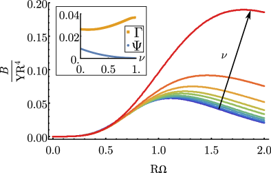
We analyze the optimal modes of deformation via the convective flow tensor, in particular, the trace ${\rm tr}(h)$ (splay) and deviatoric components $h^{\text{dev}}=h_{\alpha\beta}-{\rm tr}(h)\delta_{\alpha\beta}/2$ (biaxial splay) [30], which characterize longitudinal gradients of dilatory and shear stress in the columnar array. In contrast to a heuristic view that optimal packings should favor the uniform area per filament of splay-free textures, the inset of Fig. 3 instead shows that optimal toroids incorporate a mixture of both splay and biaxial splay where we define the respective measures of average splay and biaxial splay, $\Psi\equiv\tfrac{1}{\kappa_{0}^{2}V}\int dV\text{tr}(h)^{2}$ and $\Gamma\equiv\tfrac{1}{\kappa_{0}^{2}V}\int dV\text{tr}(h_{\text{dev}}^{2})$. Only in the incompressible limit, as $\nu\to 1$, does the splay vanish, and only at the expense of additional biaxial splay and energetic cost, implying counterintuitively that splayed textures are in fact energetically favorable in longitudinally frustrated twisted toroids. Indeed, the energetic preference for splay in non-equidistant bundles, can be traced to force balance conditions in this geometry [25].

In summary, we have shown that gauge-theoretic principles underlie the geometrically-nonlinear theory of columnar elasticity, providing a means to quantify the cost of longitudinal frustration in the mechanics of bundles. Unlike phase field models of nonlinear elasticity (such as [31, 32]), this description depends neither on the presence of a planar reference state, nor presupposes uniform crystalline order, allowing us to both accommodate the effective curvature of bundles of constant pitch helices [33], and providing a natural generalization to arbitrary target metrics [19]. Finally, because this approach to elasticity relies only on the existence of local, continuous zero modes, we note that it can be generalized to other liquid crystals, like smectics, and anticipate that it may have applications beyond liquid crystals, including mechanical metamaterials.