Mechanism design with multi-armed bandit
Abstract
A popular approach of automated mechanism design is to formulate a linear program (LP) whose solution gives a mechanism with desired properties. We analytically derive a class of optimal solutions for such an LP that gives mechanisms achieving standard properties of efficiency, incentive compatibility, strong budget balance (SBB), and individual rationality (IR), where SBB and IR are satisfied in expectation. Notably, our solutions are represented by an exponentially smaller number of essential variables than the original variables of LP. Our solutions, however, involve a term whose exact evaluation requires solving a certain optimization problem exponentially many times as the number of players, , grows. We thus evaluate this term by modeling it as the problem of estimating the mean reward of the best arm in multi-armed bandit (MAB), propose a Probably and Approximately Correct estimator, and prove its asymptotic optimality by establishing a lower bound on its sample complexity. This MAB approach reduces the number of times the optimization problem is solved from exponential to . Numerical experiments show that the proposed approach finds mechanisms that are guaranteed to achieve desired properties with high probability for environments with up to 128 players, which substantially improves upon the prior work.
1 Introduction
Multi-agent systems can be made efficient by mediators who make system-wide (social) decisions in a way that maximizes social welfare. For example, in a trading network where firms sell goods to each other or to external markets (Hatfield et al.,, 2013), the mediator can ensure that those traded goods are produced by the firms with the lowest costs and purchased by those with the highest needs (Osogami et al.,, 2023). While such mediators could maximize their own profit by charging participants (e.g., today’s tech giants who operate consumer marketplaces or ads platforms), they would typically take most of the profit, leaving the participants with only a small portion.
We instead envision an open platform whose purpose is to provide maximal benefits to the participants in multi-agent systems. This is similar to the purpose of designing an auction mechanism for public resources, which should be given to those who need them most, and there should be neither budget deficits nor surpluses on the mediator (Bailey,, 1997; Cavallo,, 2006; Dufton et al.,, 2021; Gujar and Narahari,, 2011; Guo,, 2012; Guo and Conitzer,, 2009; Manisha et al.,, 2018; Tacchetti et al.,, 2022). However, such mechanisms exploit the particular structure of single-sided auctions, where all participants are buyers, and it may be impossible to achieve desired properties in other multi-agent systems such as double-sided auctions (Hobbs et al.,, 2000; Zou,, 2009; Widmer and Leukel,, 2016; Stößer et al.,, 2010; Kumar et al.,, 2018; Chichin et al.,, 2017), matching markets (Zhang and Zhu,, 2020), and trading networks (Osogami et al.,, 2023; Wasserkrug and Osogami,, 2023) even if those properties could be guaranteed for single-sided auctions.
Here, we design mechanisms for general environments that include all these multi-agent systems, with the primary objectives of efficiency and strong budget balance (SBB). Specifically, we require that the mediator chooses a social decision such that its total value to the players (or participants) is maximized (decision efficiency; DE) and that the expected revenue of the mediator is equal to a target value, (SBB when ). As is standard in Bayesian mechanism design (Shoham and Leyton-Brown,, 2009), we assume that the value of each social decision to a player depends on the player’s type that is only known to that player, but a joint probability distribution of the players’ types is a common knowledge. Since it would be difficult to achieve DE without knowing the types, we also require that the optimal strategy of each player is to truthfully declare its type regardless of the strategies of the others (dominant strategy incentive compatibility; DSIC). To promote participation, we also require that the expected utility of each player is no less than a target value, , that can depend on the type of the player (individual rationality or IR when ).
Although these properties are standard in the literature of mechanism design (Shoham and Leyton-Brown,, 2009), here we have introduced parameters, and , to generalize the standard definitions of SBB () and IR () with three motivations. First, it is not always possible to achieve the four desired properties with the standard definitions of IR and SBB (Green and Laffont,, 1977; Myerson and Satterthwaite,, 1983; Osogami et al.,, 2023), while the generalization will enable the exact characterization of when those properties can be satisfied. Second, this generalization will allow us to develop a principled approach of learning a mechanism, where some of the quantities are estimated from samples, with theoretical guarantees. The mechanism designed with our learning approach can be shown to satisfy the four desired properties with high probability. Finally, the additional parameters will allow us to model practical requirements. For example, the mediator might need positive revenue to cover the cost of maintaining the platform or might want to guarantee positive expected utility to players to encourage participation in this platform rather than others.
We require SBB and IR in expectation (ex ante or interim) with respect to the distribution of types, while DE and DSIC are satisfied for any realization of types (ex post). While these assumptions are similar to those in Osogami et al., (2023); Wasserkrug and Osogami, (2023) for trading networks, the in expectation properties are certainly weaker than the ex post properties usually assumed for auctions (Bailey,, 1997; Cavallo,, 2006; Dufton et al.,, 2021; Gujar and Narahari,, 2011; Guo,, 2012; Guo and Conitzer,, 2009; Manisha et al.,, 2018; Tacchetti et al.,, 2022). With the weaker properties, however, we derive analytical solutions of the mechanisms that satisfy all the four desired properties in the general environments (and characterize when those properties can be satisfied). This is in stark contrast to the prior work, where mechanisms are analytically derived only for auctions with a single type of goods (Bailey,, 1997; Cavallo,, 2006; Guo,, 2011; Guo and Conitzer,, 2007, 2009; Moulin,, 2009) or with unit demand (Gujar and Narahari,, 2011; Guo,, 2012). For more complex auctions (Dufton et al.,, 2021; Manisha et al.,, 2018; Tacchetti et al.,, 2022) or trading networks (Osogami et al.,, 2023; Wasserkrug and Osogami,, 2023), mechanisms are computed by numerically solving optimization problems, whose size often grows exponentially with the number of players.
While the numerical approaches proposed in Osogami et al., (2023) have been applied only to the trading networks with two players, our analytical solutions can be evaluated numerically with players, depending on the number of types. The key bottleneck in our analytical solutions lies in the evaluation of the minimum expected value over possible types of each player. Exact evaluation of this quantity would require computing an efficient social decision for all the combinations of types, where is the number of possible types of each player, and is the number of players.
To overcome this bottleneck, we model the problem of evaluating this minimum expected value in a multi-armed bandit (MAB) approach (Lattimore and Szepesvári,, 2020) and propose an asymptotically optimal learning algorithm for this problem. While the standard objectives of MAB are regret minimization (Auer et al.,, 1995, 2002) and best arm identification (Audibert et al.,, 2010; Maron and Moore,, 1993; Mnih et al.,, 2008; Bubeck et al.,, 2009), our objective is to estimate the mean reward of the best arm. We propose a probably approximately correct (PAC) algorithm, which approximately (with error at most ) estimates the best mean with high probability (at least ), and proves that its sample complexity, , matches the lower bound that we derive. This learning approach substantially reduces the number of computing efficient social decisions from to , enabling us to numerically find mechanisms for players, depending on .
Our contributions thus revolve around the optimization problem whose solution gives the mechanism that satisfies DE, SBB, DSIC, and IR (see Section 3-4). First, we establish a sufficient condition that ensures the optimization problem has feasible solutions, and prove that this sufficient condition is also necessary when the players have independent types (see Section 5). Second, for cases where this sufficient condition holds, we analytically derive a class of optimal solutions to this optimization problem, which in turn gives mechanisms that satisfy DE, SBB, DSIC, and IR for general environments including auctions and trading networks (see Section 5). Third, we model the problem of evaluating a quantity in the above analytical expressions as best mean estimation in MAB, propose a PAC algorithm for this problem, and prove its asymptotic optimality (see Section 6). Finally, we empirically validate the effectiveness of the proposed approach (see Section 7). In Section 2, we start by positioning our contributions to the prior work.
2 Related work
The prior work most related to ours is Osogami et al., (2023), which formulates and numerically solves the LP whose solution gives the mechanism for a trading network that satisfies DE, DSIC, IR, and weak budget balance (WBB; expected revenue of the mediator is nonnegative). While the objective of the LP is rather arbitrary and SBB is given just as an example in Osogami et al., (2023), we focus on SBB and drive analytical solutions for this particular objective. Our formulation extends Osogami et al., (2023) with additional parameters and notations that cover environments beyond trading networks, but these extensions are relatively straightforward.
In the rest of this section, we discuss related work on mechanism design, with a focus on those aiming to achieve SBB, as well as related work on MAB with a focus on PAC algorithms. In particular, we will see that our learning approach is unique in that we estimate a particular quantity in the optimal solution that we derive analytically, and this leads us to propose a new PAC algorithm and establish its optimality for an underexplored objective of best mean estimation in MAB.
In single-sided auctions where only buyers make strategic decisions, Vickrey–Clarke–Groves (VCG) mechanisms with Clark’s pivot rule (also called VCG auction) satisfy ex post DE (called allocative efficiency in auctions), DSIC, IR, and WBB (Nisan,, 2007). However, the Green-Laffont Impossibility Theorem implies that no mechanism can guarantee DE, DSIC, and SBB simultaneously for all environments (Green and Laffont,, 1977, 1979). This has led to a series of work on redistributing the revenue of the mediator to the players as much as possible (i.e., to make budget balance as strong as possible), while satisfying DSIC, DE, IR, and WBB. For auctions with single or homogeneous goods (Bailey,, 1997; Cavallo,, 2006; Guo,, 2011; Guo and Conitzer,, 2007, 2009; Moulin,, 2009) or for auctions where players have unit demand (Gujar and Narahari,, 2011; Guo,, 2012), researchers have derived analytical solutions that optimally redistribute the payment to the players. For auctions with multi-unit demands on heterogeneous goods, the prior work has proposed numerical approaches that seek to find the piecewise linear functions (Dufton et al.,, 2021) or neural networks (Manisha et al.,, 2018; Tacchetti et al.,, 2022) that best approximate the optimal redistribution functions.
We consider the environments that not only allow heterogeneous goods and multi-unit demands but also are more general than single-sided auctions. In particular, our players may have negative valuation on a social decision. The Myerson-Satterthwaite Impossibility Theorem (Myerson and Satterthwaite,, 1983) thus implies that, unlike VCG auctions, no mechanism can guarantee ex post DE, DSIC, IR, and WBB simultaneously for all the environments that we consider. We thus derive mechanisms that achieve DE, DSIC, IR, and SBB in the best possible manner. A limitation of our results is that IR and SBB are satisfied only in expectation. Such a guarantee in expectation can however be justified for risk-neutral mediator and players (Osogami et al.,, 2023). Our model can also guarantee strictly positive expected utility, which in turn can ensure nonnegative utility with high probability when the player repeatedly participate in the mechanism.
For auctions, there also exists a large body of the literature on maximizing the revenue of the mediator (Myerson,, 1981) with recent focus on automated mechanism design (AMD) with machine learning (Duetting et al.,, 2019; Rahme et al.,, 2021; Ivanov et al.,, 2022; Curry et al.,, 2020) and analysis of its sample complexity (Balcan et al.,, 2016; Morgenstern and Roughgarden,, 2015; Syrgkanis,, 2017). Similar to these and other studies of AMD (Sandholm,, 2003; Conitzer and Sandholm,, 2002), we formulate an optimization problem whose solution gives the mechanism with desired properties. However, instead of solving it numerically, we analytically derive optimal solutions. Also, while the prior work analyzes the sample complexity for finding the mechanism that maximizes the expected revenue, we analytically find optimal mechanisms and characterize the sample complexity of evaluating a particular expression in the analytically designed mechanisms.
We evaluate our analytical expression through best mean estimation (BME) in MAB, where the standard objectives are regret minimization (Auer et al.,, 1995, 2002) and best arm identification (BAI) (Audibert et al.,, 2010; Maron and Moore,, 1993; Mnih et al.,, 2008; Bubeck et al.,, 2009). The prior work on MAB that is most relevant to ours is PAC learning for BAI and analysis of its sample complexity. We reduce the problem of BME to BAI and prove the lower bound on the sample complexity of BME using a technique known for BAI (Even-Dar et al.,, 2002). However, while this technique does not give tight lower bound for BAI (Mannor and Tsitsiklis,, 2004), we show that it gives tight lower bound for BME. Notice that the problem of estimating the best mean frequently appears in reinforcement learning (van Hasselt,, 2010) and machine learning (Kajino et al.,, 2023), but there the focus is on how best to estimate the best mean with a given set of samples (van Hasselt,, 2013), while our focus is on how best to collect samples to estimate the best mean.
3 Settings
The goal of mechanism design is to specify the rules of a game in a way that an outcome desired by the mechanism designer is achieved when rational players (i.e., players whose goal it is to maximize their individual utility) participate in that game (Jackson,, 2014; Shoham and Leyton-Brown,, 2009). Formally, let be the set of players and be the set of possible outcomes. For each player , let be the set of available actions and be the set of possible types. Let and be the corresponding product spaces. A mechanism determines an outcome depending of the actions taken by the players. Let be the utility function of each player .
We consider Bayesian games where the players’ types follow a probability distribution that is known to all players and the mediator. Before selecting actions, the players know their own types but not the types of the other players. A strategy of each player is thus a function from to .
We assume that an outcome is determined by a social decision and payment; hence, a mechanism consists of a decision rule and a payment rule. Let be the set of possible social decisions. Given the actions of the players, the decision rule determines a social decision, and the payment rule determines the amount of (possibly negative) payment to the mediator from each player. Let specify the value of a given social decision to the player of a given type. Then the utility of player when players take actions is
| (1) |
Throughout, we assume that , , and are finite sets.
Without loss of generality by the revelation principle (Shoham and Leyton-Brown,, 2009), we consider only direct mechanisms, where the action available to each player is to declare which type the player belongs to from the set of possible types (i.e., ). We will thus use for .
Then we seek to achieve the following four properties with our mechanisms. The first property is Dominant Strategy Incentive Compatibility (DSIC), which ensures that the optimal strategy of each player is to truthfully reveal its type regardless of the strategies of the other players. Formally, {fleqn}
| (2) |
where the left-hand side represents the utility of the player having type when it declares the same , and the other players declare arbitrary types .
The second property is Decision Efficiency (DE), which requires that the mediator chooses the social decision that maximizes the total value to the players. With DSIC, we can assume that the players declare true types, and hence we can write DE as a condition on the decision rule: {fleqn}[10pt]
| (3) |
As the third property, we generalize individual rationality and require that the expected utility of each player is at least as large as a target value that can depend on its type. We refer to this property as -IR. Again, assuming that players declare true types due to DSIC, we can write -IR as follows: {fleqn}[10pt]
| (4) |
where determines the target expected utility for each type. Throughout (except in Section 6, where we discuss general MAB models), denotes the expectation with respect to the probability distribution of types, which is the only probability that appears in our mechanisms.
The last property is a generalization of Budget Balance (BB), which we refer to as -WBB and -SBB. Specifically, -WBB requires that the expected revenue of the mediator is no less than a given constant , and -SBB requires that it is equal to . Again, assuming that the players declare true types due to DSIC, these properties can be written as follows: {fleqn}[10pt]
| (5) |
While -SBB is stronger than -WBB, we will see that -SBB is satisfiable iff -WBB is satisfiable.
4 Optimization problem for automated mechanism design
Following Osogami et al., (2023), we seek to find optimal mechanisms in the class of VCG mechanisms. A VCG mechanism is specified by a pair . Specifically, after letting player take the actions of declaring their types , the mechanism first finds a social decision using a decision rule that satisfies DE (3). It then determines the amount of payment from each player to the mediator by
| (6) |
where we define , and is an arbitrary function of the types of the players other than and referred to as a pivot rule. The decision rule guarantees DE (3) by construction, and the payment rule (6) then guarantees DSIC (2) (Nisan,, 2007).
Our problem is now reduced to find the pivot rule, , that minimizes the expected revenue of the mediator, while satisfying -IR and -WBB. This may lead to satisfying -SBB if the revenue is maximally reduced. To represent this reduced problem, let
| (7) |
be the total value of the efficient social decision when the players have types . Then we can rewrite -IR (for the player having type ) and -WBB as follows (see Appendix A.1 for full derivation):
| (8) | ||||
| (9) |
Therefore, we arrive at the following linear program (LP):
| (10) | ||||
| (11) | ||||
| (12) |
The approach of Osogami et al., (2023) is to numerically solve this LP possibly with approximations. Since is a variable for each and each , the LP has variables and constraints, when each player has possible types. When this LP is feasible, let be its optimal solution; then the VCG mechanism guarantees DSIC, DE, -IR, and -WBB (formalized as Proposition 4 in Appendix A.1). Otherwise, no VCG mechanisms can guarantee them all. In the next section, we characterize exactly when the LP is feasible and provide analytical solutions to the LP.
5 Analytical solution to the optimization problem
We first establish a sufficient condition and a necessary condition for the LP to have feasible solutions. Note that complete proofs for all theoretical statements are provided in Appendix B.
Lemma 2.
These two lemmas establish the following necessary and sufficient condition.
While the LP is not necessarily feasible, one may choose and in a way that it is guaranteed to be feasible. For example, the feasibility is guaranteed (i.e., (13) is satisfied) by setting
| (14) |
where for . When , the mediator might get negative expected revenue, but the expected loss of the mediator is at most . Appendix A.2 provides alternative and that guarantee feasibility, but some of the players might incur negative expected utility.
Finally, we derive a class of optimal solutions to the LP when it is feasible.
Lemma 3.
When types are independent, the condition (13) is necessary for the existence of a feasible solution; hence, we do not lose optimality by considering only the solutions in . On the other hand, when types are dependent, the condition (13) may still be satisfied, where the solutions in remain optimal. However, dependent types no longer necessitate (13) to satisfy (11)-(12); hence the space of constant pivot rules may not suffice to find an optimal solution if (13) does not hold.
Proposition 1.
Corollary 2.
In deriving the optimal solutions, we have substantially reduced the essential number of variables (from to when each player has types). Our approach can therefore not only find but also represent or store solutions exponentially more efficiently than Osogami et al., (2023).
It turns out that the solutions in not only satisfy -WBB but also -SBB (in addition to DE, DSIC, and -IR) regardless of whether the types are independent or not:
Corollary 3.
Any VCG mechanism given with a pivot rule in satisfies -SBB.
When the LP is infeasible, we can construct a mechanism that satisfies one of -SBB and -IR (in addition to DE and DSIC) regardless of whether the types are independent or not:
For example, for any and , the following pivot rule always satisfies -IR:
| (18) |
where we define (see also (58) in the appendix)
| (19) |
So far, we have analytically derived the class of optimal solutions for the LP. Although these analytical solutions substantially reduce the computational cost of solving the LP compared to the numerical solutions in Osogami et al., (2023), they still need to evaluate
| (20) |
for each . Since is the expectation with respect to the distribution over , this would require evaluating for all . Recall that defined with (7) is the total value of the efficient decision , which is given by a solution to an optimization problem (3). Without any structure in and , this would require evaluating the total value for all decisions in .
6 Online learning for evaluating the analytical solution
To alleviate the computational complexity associated with (20), we propose a learning approach. A key observation is that the problem of estimating (20) can be considered as a variant of a multi-armed bandit (MAB) problem whose objective is to estimate the mean reward of the best arm. Specifically, the MAB gives the reward when we pull an arm , where is a sample from the conditional distribution . Following the relevant prior work on MAB (Even-Dar et al.,, 2002, 2006; Hassidim et al.,, 2020; Mannor and Tsitsiklis,, 2004), we maximize reward in this section.
Since we assume that , , and are finite, there exist constants, and , such that and . Then we can also bound . Namely, the reward in the MAB is bounded. We assume that we know the bounds on the reward and can scale it such that the scaled reward is in surely.
We also assume that we have access to an arbitrary size of the sample that is independent and identically distributed (i.i.d.) according to for any . When players have independent types, such sample can be easily constructed as long as we have access to i.i.d. sample from , because is the sample from for any .
Consider the general -armed bandit where the reward of each arm is bounded in . For each , let be the true mean of arm . Let be the best mean-reward, which we want to estimate. We say that the sample complexity of an algorithm for a MAB is if the sample size needed by the algorithm is bounded by (i.e., arms are pulled at most times).
A standard Probably Approximately Correct (PAC) algorithm for MAB returns an -optimal arm with probability at least for given (Even-Dar et al.,, 2006; Hassidim et al.,, 2020). We will use the following definition:
Definition 1 (()-PAC Best Arm Identifier (Even-Dar et al.,, 2006)).
For , we say that an algorithm is ()-PAC Best Arm Identifier (BAI) if the arm identified by the algorithm satisfies
| (21) |
Definition 2 (()-PAC Best Mean Estimator).
For , we say that an algorithm is ()-PAC Best Mean Estimator (BME) if the best mean estimated by the algorithm satisfies
| (22) |
BAI and BME are related but different. For example, consider the case where the best arm has large variance and , and the other arms always give zero reward . Then relatively small sample would suffice for BAI due to the large gap , while BME would require relatively large sample due to the large variance of the best arm . As another example, consider the case where we have many arms whose rewards follow Bernoulli distributions. Suppose that half of the arms have an expected value of 1, and the other half have an expected value of . Then by pulling sufficiently many arms (once for each arm), we can estimate that the best mean is at least with high probability (by Hoeffding’s inequality), but BAI would require pulling arms sufficiently many times until we pull one of the best arms sufficiently many times (to be able to say that this particular arm has an expected value at least ).
For ()-PAC BAI, the following lower and upper bounds on the sample complexity are known:
Proposition 2 (Mannor and Tsitsiklis, (2004)).
There exists a ()-PAC BAI with sample complexity , and any ()-PAC BAI must have the sample complexity at least .
We establish the same lower and upper bounds for ()-PAC BME:
Theorem 1.
There exists a ()-PAC BME with sample complexity , and any ()-PAC BME must have the sample complexity at least .
Our upper bound is established by reducing BME to BAI. Suppose that we have access to an arbitrary -PAC BAI with sample complexity (Algorithm 2 in Appendix A.3). We can construct a -PAC BME by first running the -PAC BAI and then sampling from the arm that is identified as the best until we have a sufficient number, , of samples from (Algorithm 3 in Appendix A.3). When is appropriately selected, the following lemma holds:
Lemma 4.
When a -PAC BAI with sample complexity is used, Algorithm 3 has sample complexity , where , and returns that satisfies
| (23) |
Our lower bound is established by showing that an arbitrary -PAC BME can be used to solve the problem of identifying whether a given coin is negatively or positively biased (precisely, -Biased Coin Problem of Definition 3 in Appendix A.3), for which any algorithm is known to require expected sample complexity at least to solve correctly with probability at least (Chernoff,, 1972; Even-Dar et al.,, 2002) (see Lemma 7 in Appendix A.3). The following lemma, together with Lemma 7, establishes the lower bound on the sample complexity in Theorem 1:
Lemma 5.
If there exists an -PAC BME with sample complexity for -armed bandit, then there also exists an algorithm, having expected sample complexity , that can solve the -Biased Coin Problem correctly with probability at least .
We prove Lemma 5 by reducing the -Biased Coin Problem to BME. This proof technique was also used in Even-Dar et al., (2002) to prove a lower bound on the sample complexity of BAI. What is interesting, however, is that the lower bound in Even-Dar et al., (2002) is not tight when , and a tight lower bound is established by a different technique in Mannor and Tsitsiklis, (2004). On the other hand, our proof gives a tight lower bound on the sample complexity of BME. In Appendix A.3, we further discuss where this difference in the derived lower bounds comes from.
Finally, we connect the results on BME back to our mechanism in Section 5 and provide a guarantee on the properties of the mechanism when the term (20) is estimated with BME. To this end, we define the terms involving expectations in Lemma 3 as follows:
| (24) | ||||
| (25) |
Then, recalling that is the number of players, we have the following lemma:
Lemma 6.
Let for and be independent estimates of and respectively given by an -PAC Best Mean Estimator and a standard -PAC estimator of expectation. Also, let be a point on the following simplex (here, we change the notation from in Lemma 3 to to avoid confusion):
| (26) | ||||
| (27) |
Then the VCG mechanism with the constant pivot rule satisfies -IR and -WBB with probability .
Notice that the sufficient condition of Lemma 1 states that the simplex in Lemma 3 is nonempty. Analogously, when the simplex in Lemma 6 is empty, we cannot provide the solution that guarantees the properties stated in Lemma 6. Since DSIC and DE remain satisfied regardless of whether for and are estimated or exactly computed, Lemma 6 immediately establishes the following theorem by appropriately choosing the parameters:
Theorem 2.
In Lemma 6, let , , and . Then the VCG mechanism with the constant pivot rule satisfies DSIC, DE, -IR, and -WBB with probability .
Recall that the exact computation of our mechanism in Lemma 3 requires evaluating for all , whose size grows exponentially with the number of players, . Our BME algorithm reduces this requirement to , as is formally proved in the following proposition:
Proposition 3.
The sample complexity to learn the constant pivot rule in Theorem 2 is , where is the number of players, and is the maximum number of types of each player.
7 Numerical experiments
We conduct several numerical experiments to validate the effectiveness of the proposed approach and to understand its limitations. Specifically, we design our experiments to investigate the following questions. i) BME studied in Section 6 has asymptotically optimal sample complexity, but how well can we estimate the best mean when there are only a moderate number of arms? ii) How much can BME reduce the number of times given by (7) is evaluated? iii) How well -IR and -SBB are satisfied when (20) is estimated by BME rather than calculated exactly? In this section, we only provide a brief overview of our experiments; for full details, see Appendix A.4. In particular, we find the key empirical property of BME that it can reduce the computational complexity by many orders of magnitude when the number of players is moderate () to large but is relatively less effective against the increased number of types.
For question i), we compare Successive Elimination for BAI (SE-BAI), which is known to perform well for a moderate number of arms (Hassidim et al.,, 2020; Even-Dar et al.,, 2006), against the corresponding algorithm for BME (SE-BME) and summarize the results in Appendix A.4.1. Overall, we find that SE-BME generally requires smaller sample size than SE-BAI, except when there are only a few arms and their means have large gaps. The efficiency of SE-BAI for this case makes intuitive sense, since the best arm can be identified without estimating the means with high accuracy.

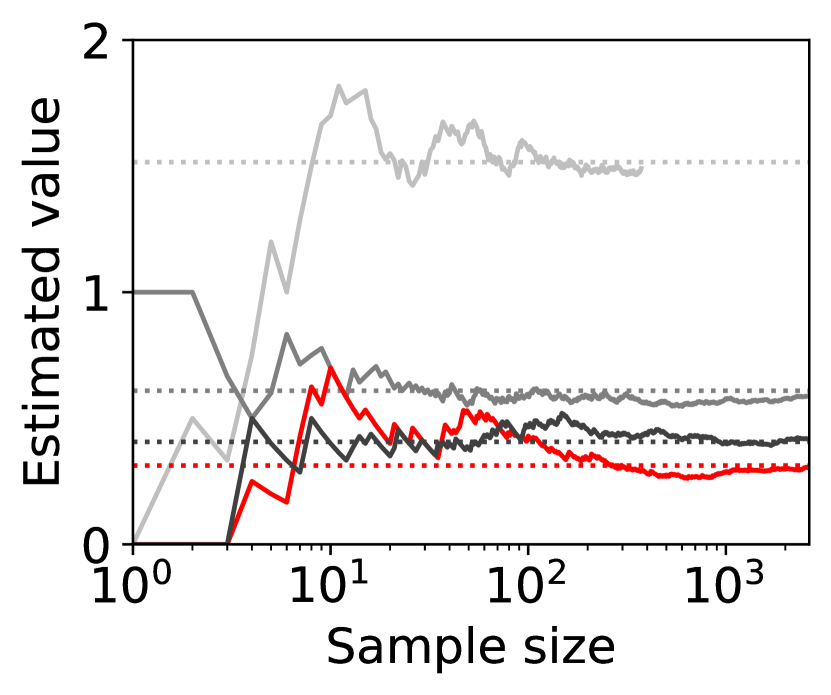
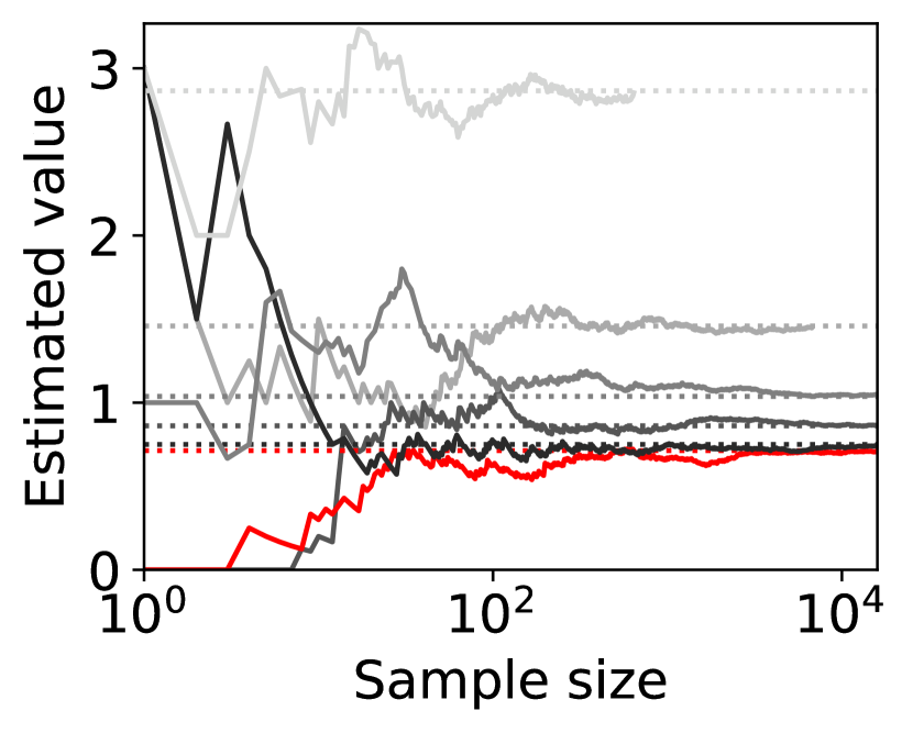
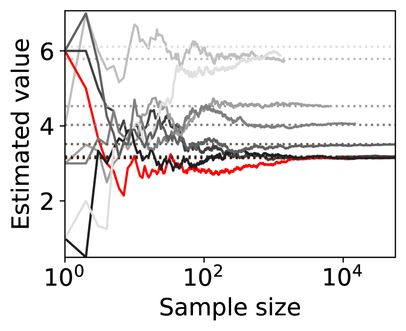
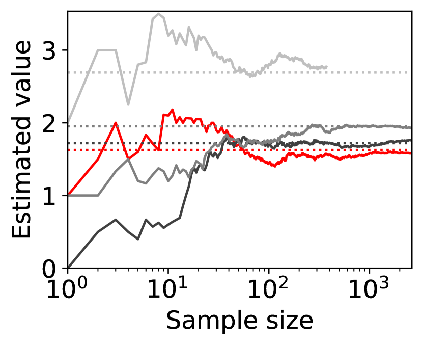
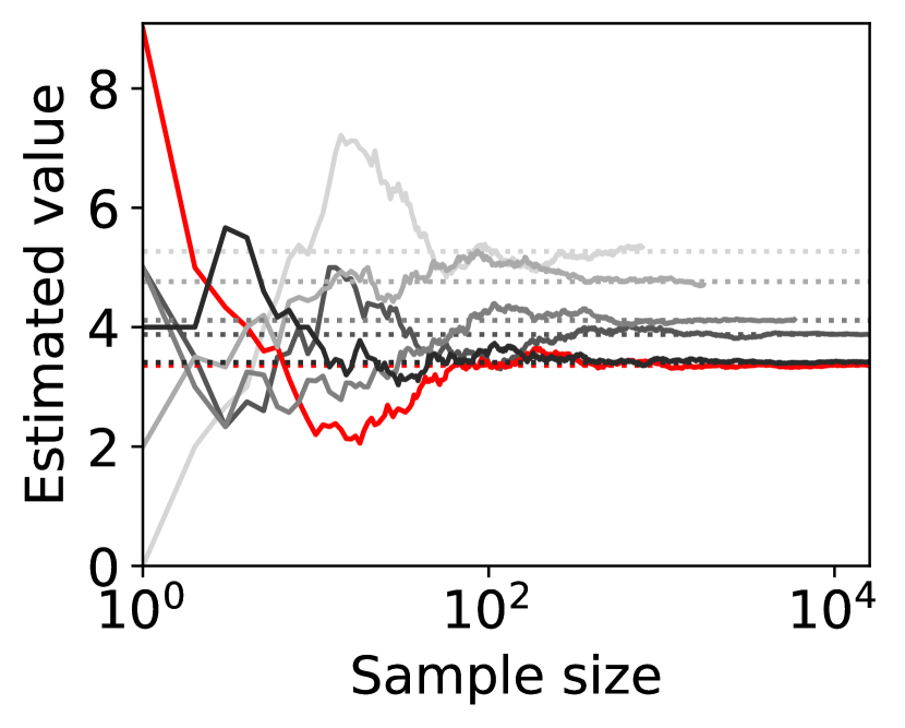
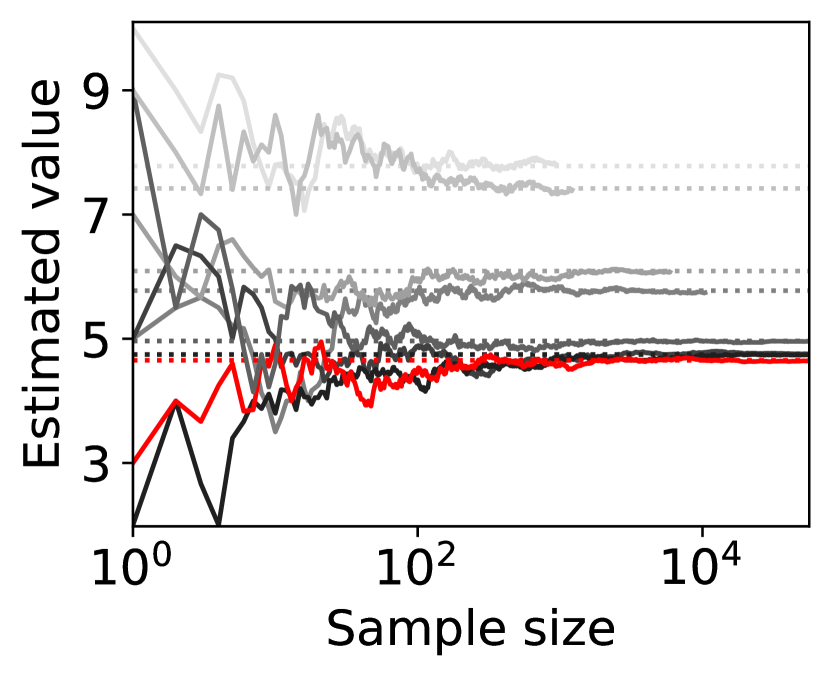
(a) sample path
(b) sample size against

(c) sample size against
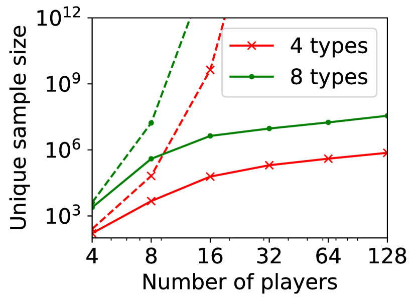
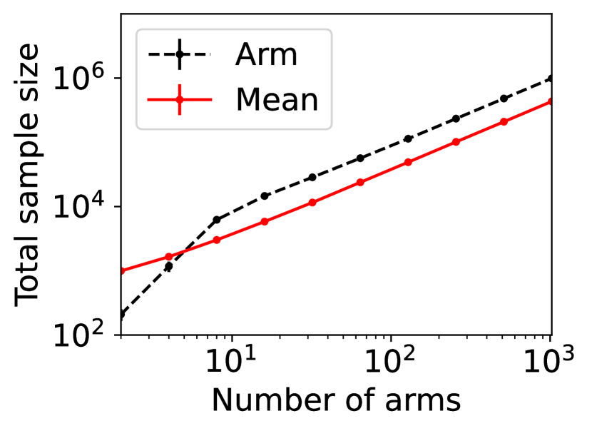
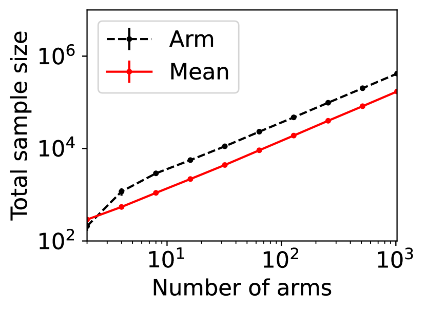
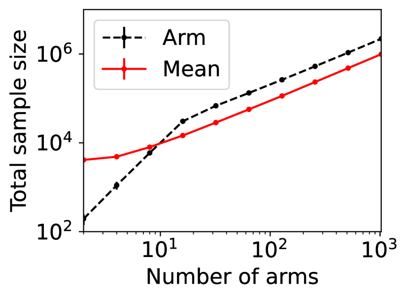
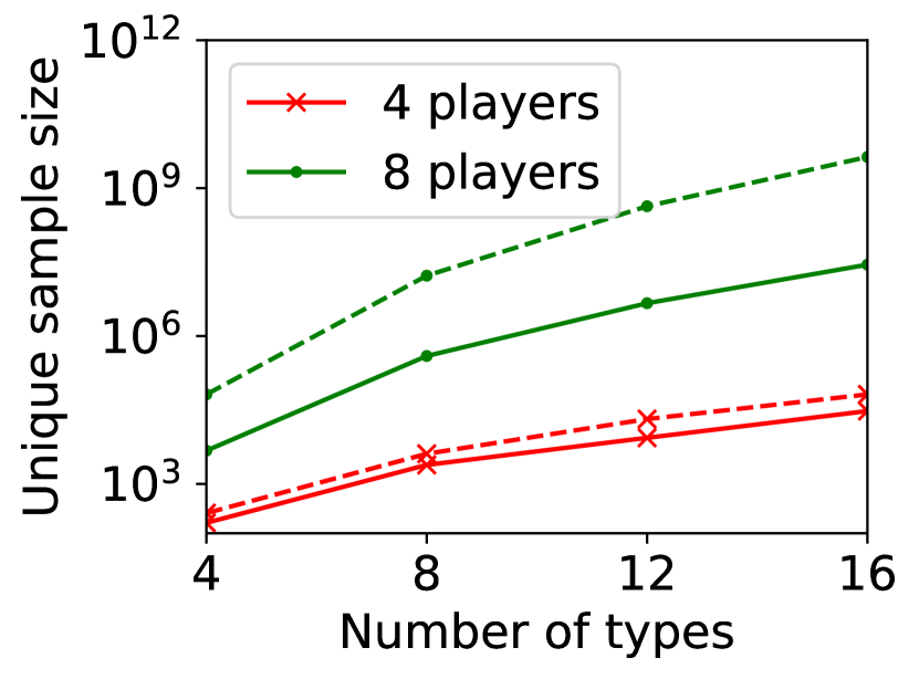
For question ii), we quantitatively validate the effectiveness of SE-BME in reducing the number of times is computed when we evaluate (20) in a setting of mechanism design, as is detailed in Appendix A.4.2. Figure 1 summarizes the results. Panel (a) shows that the means close to the minimum value are estimated with high accuracy, while others are eliminated by SE-BME after a small number of samples. Panels (b)-(c) show that SE-BME (solid curves) evaluates by orders of magnitude smaller number of times than what is required by exact computation (dashed curves). The effectiveness of SE-BME is particularly striking when (the number of players) grows. While exact computation evaluates exponentially many times as grows, SE-BME has only linear dependency on . This insensitivity of the sample complexity of SE-BME to makes intuitive sense, since only affects the distribution of the reward and keeps the number of arms unchanged.
(a) players’ utility

(b) mediator’s revenue

(c) players’ utility

(d) mediator’s revenue
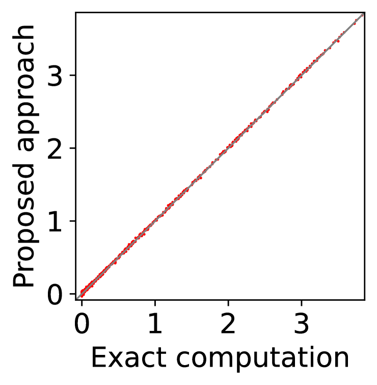
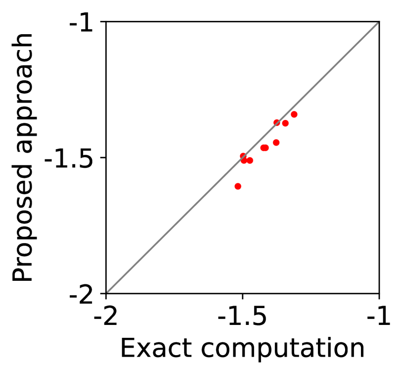
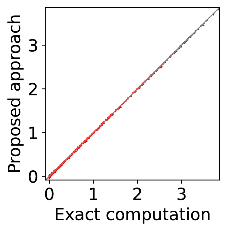
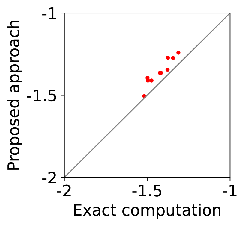
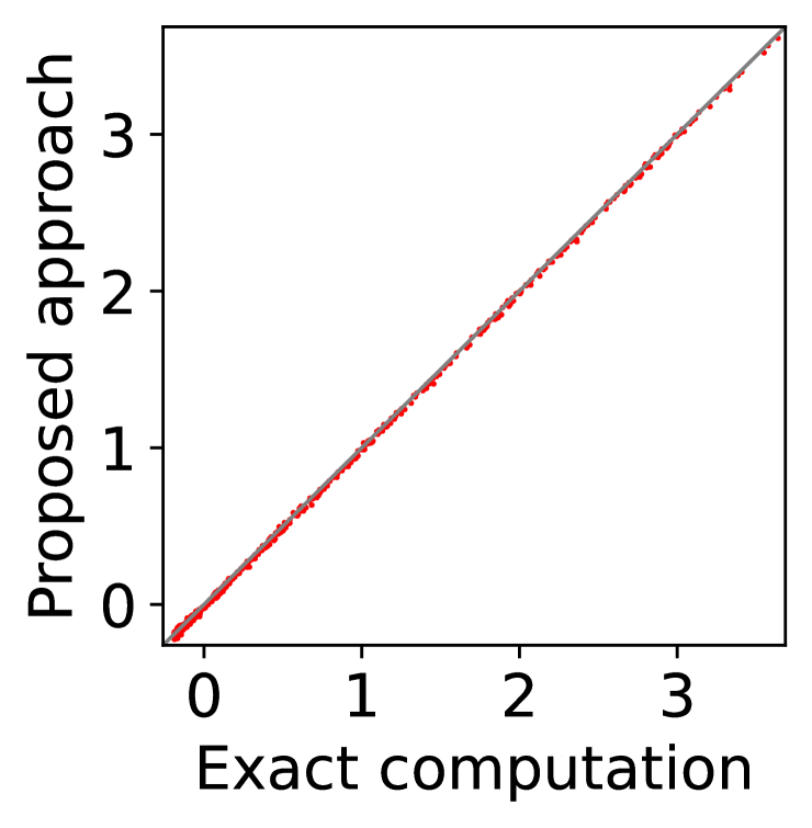
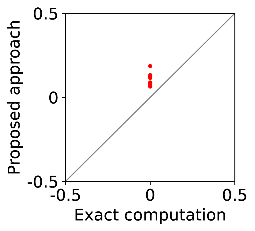
For question iii), we quantitatively evaluate how well -IR and -SBB are guaranteed when we estimate (20) with SE-BME, where we continue to use the same setting of mechanism design. In Figure 2, we study two analytical solutions: one guarantees to satisfy -IR (with ), and the other guarantees to satisfy -SBB (with ). The red dots show the expected utility of the players in (a) and (c) as well as the expected revenue of the mediator in (b) and (d), when (20) is evaluated either exactly (horizontal axes) or estimated with SE-BME (vertical axes). Overall, the expected revenue of the mediator is more sensitive than the expected utility of the players to the error in the estimation of (20), because (12) involves the summation , while (11) only involves for a single . We can however ensure that -WBB (instead of SBB) is satisfied with high probability by replacing the with a when we compute after (20) is estimated. As we show and explain with Figure 8 in Appendix A.4.3, this will simply shift the dots in the figure, and we can guarantee -WBB with high probability with an appropriate selection of .
We have run all of the experiments on a single core with at most 66 GB memory without GPUs in a cloud environment, as is detailed in Appendix A.4.4. The associated source code is submitted as a supplementary material and will be open-sourced upon acceptance.
8 Conclusion
We have analytically derived optimal solutions for the LP that gives mechanisms that guarantee the desired properties of DE, DSIC, -SBB, and -IR. When there are players, each with possible types, the LP involves variables, while our analytical solutions are represented by only essential variables. While Osogami et al., (2023) numerically solves this LP only for , we have exactly evaluated our analytical solutions for (see Figure 1). The analytical solution, however, involves a term whose exact evaluation requires finding efficient social decisions times. We have modeled the problem of evaluating this term as best mean estimation in multi-armed bandit, proposed a PAC estimator, and proved its asymptotic optimality by establishing a lower bound on the sample complexity. Our experiments show that our PAC estimator enables finding mechanism for and with a guarantee on the desired properties.
The proposed approach makes a major advancement in the field and can positively impact society by providing guarantees on desired properties for large environments, which existing approaches are unable to handle. However, it presents certain limitations and potential challenges, which inspire several directions for further research. Regarding limitations, one should keep in mind that our mechanisms guarantee -SBB and -IR only in expectation, and that the our approaches have only been applied to the environments up to 128 players and up to 16 types in our experiments. Regarding societal impacts, our approach might result in the mechanisms that are unfair to some of the players, because DE does not mean that all of the players are treated fairly. These limitations and societal impacts are further discussed in Appendix A.5.
References
- Audibert et al., (2010) Audibert, J., Bubeck, S., and Munos, R. (2010). Best arm identification in multi-armed bandits. In Kalai, A. T. and Mohri, M., editors, Proceedings of the 23rd Conference on Learning Theory, pages 41–53. Omnipress.
- Auer et al., (1995) Auer, P., Cesa-Bianchi, N., Freund, Y., and Schapire, R. (1995). Gambling in a rigged casino: The adversarial multi-armed bandit problem. In Proceedings of IEEE 36th Annual Foundations of Computer Science, pages 322–331.
- Auer et al., (2002) Auer, P., Cesa-Bianchi, N., and P., F. (2002). Finite-time analysis of the multiarmed bandit problem. Machine Learning, 47:235––256.
- Bailey, (1997) Bailey, M. J. (1997). The demand revealing process: To distribute the surplus. Public Choice, 91(2):107–126.
- Balcan et al., (2016) Balcan, M.-F., Sandholm, T., and Vitercik, E. (2016). Sample complexity of automated mechanism design. In Proceedings of the 30th International Conference on Neural Information Processing Systems, NIPS’16, page 2091–2099, Red Hook, NY, USA. Curran Associates Inc.
- Bubeck et al., (2009) Bubeck, S., Munos, R., and Stoltz, G. (2009). Pure exploration in multi-armed bandits problems. In Gavaldà, R., Lugosi, G., Zeugmann, T., and Zilles, S., editors, Algorithmic Learning Theory, pages 23–37, Berlin, Heidelberg. Springer Berlin Heidelberg.
- Cavallo, (2006) Cavallo, R. (2006). Optimal decision-making with minimal waste: Strategyproof redistribution of VCG payments. In Proceedings of the Fifth International Joint Conference on Autonomous Agents and Multiagent Systems, AAMAS ’06, page 882–889, New York, NY, USA. Association for Computing Machinery.
- Chernoff, (1972) Chernoff, H. (1972). Sequential Analysis and Optimal Design. CBMS-NSF Regional Conference Series in Applied Mathematics, Series Number 8. Society for Industrial and Applied Mathematics.
- Chichin et al., (2017) Chichin, S., Vo, Q. B., and Kowalczyk, R. (2017). Towards efficient and truthful market mechanisms for double-sided cloud markets. IEEE Transactions on Services Computing, 10(1):37–51.
- Conitzer and Sandholm, (2002) Conitzer, V. and Sandholm, T. (2002). Complexity of mechanism design. In Proceedings of the 18th Conference on Uncertainty in Artificial Intelligence, page 103–110.
- Curry et al., (2020) Curry, M., Chiang, P.-Y., Goldstein, T., and Dickerson, J. (2020). Certifying strategyproof auction networks. In Larochelle, H., Ranzato, M., Hadsell, R., Balcan, M., and Lin, H., editors, Advances in Neural Information Processing Systems, volume 33, pages 4987–4998. Curran Associates, Inc.
- Duetting et al., (2019) Duetting, P., Feng, Z., Narasimhan, H., Parkes, D., and Ravindranath, S. S. (2019). Optimal auctions through deep learning. In Chaudhuri, K. and Salakhutdinov, R., editors, Proceedings of the 36th International Conference on Machine Learning, volume 97 of Proceedings of Machine Learning Research, pages 1706–1715. PMLR.
- Dufton et al., (2021) Dufton, L., Naroditskiy, V., Polukarov, M., and Jennings, N. (2021). Optimizing payments in dominant-strategy mechanisms for multi-parameter domains. Proceedings of the AAAI Conference on Artificial Intelligence, 26(1):1347–1354.
- Even-Dar et al., (2002) Even-Dar, E., Mannor, S., and Mansour, Y. (2002). PAC bounds for Multi-armed bandit and Markov decision processes. In Kivinen, J. and Sloan, R. H., editors, Computational Learning Theory, pages 255–270, Berlin, Heidelberg. Springer Berlin Heidelberg.
- Even-Dar et al., (2006) Even-Dar, E., Mannor, S., and Mansour, Y. (2006). Action elimination and stopping conditions for the multi-armed bandit and reinforcement learning problems. Journal of Machine Learning Research, 7(39):1079–1105.
- Green and Laffont, (1977) Green, J. R. and Laffont, J. J. (1977). Characterization of satisfactory mechanism for the revelation of preferences for public goods. Econometrica, 45:427–438.
- Green and Laffont, (1979) Green, J. R. and Laffont, J.-J. (1979). Incentives in Public Decision Making. North-Holland Publishing Company, Amsterdam.
- Gujar and Narahari, (2011) Gujar, S. and Narahari, Y. (2011). Redistribution mechanisms for assignment of heterogeneous objects. Journal of Artificial Intelligence Research, 41(2):131–154.
- Guo, (2011) Guo, M. (2011). VCG redistribution with gross substitutes. Proceedings of the AAAI Conference on Artificial Intelligence, 25(1):675–680.
- Guo, (2012) Guo, M. (2012). Worst-case optimal redistribution of VCG payments in heterogeneous-item auctions with unit demand. In Proceedings of the 11th International Conference on Autonomous Agents and Multiagent Systems - Volume 2, AAMAS ’12, page 745–752, Richland, SC. International Foundation for Autonomous Agents and Multiagent Systems.
- Guo and Conitzer, (2007) Guo, M. and Conitzer, V. (2007). Worst-case optimal redistribution of VCG payments. In Proceedings of the 8th ACM Conference on Electronic Commerce, EC ’07, page 30–39, New York, NY, USA. Association for Computing Machinery.
- Guo and Conitzer, (2009) Guo, M. and Conitzer, V. (2009). Worst-case optimal redistribution of VCG payments in multi-unit auctions. Games and Economic Behavior, 67(1):69–98. Special Section of Games and Economic Behavior Dedicated to the 8th ACM Conference on Electronic Commerce.
- Hassidim et al., (2020) Hassidim, A., Kupfer, R., and Singer, Y. (2020). An optimal elimination algorithm for learning a best arm. In Larochelle, H., Ranzato, M., Hadsell, R., Balcan, M., and Lin, H., editors, Advances in Neural Information Processing Systems, volume 33, pages 10788–10798. Curran Associates, Inc.
- Hatfield et al., (2013) Hatfield, J. W., Kominers, S. D., Nichifor, A., Ostrovsky, M., and Westkamp, A. (2013). Stability and competitive equilibrium in trading networks. Journal of Political Economy, 121(5):966–1005.
- Hobbs et al., (2000) Hobbs, B. F., Rothkopf, M. H., Hyde, L. C., and O’Neill, R. P. (2000). Evaluation of a truthful revelation auction in the context of energy markets with nonconcave benefits. Journal of Regulatory Economics, 18:5–32.
- Ivanov et al., (2022) Ivanov, D., Safiulin, I., Filippov, I., and Balabaeva, K. (2022). Optimal-er auctions through attention. In Oh, A. H., Agarwal, A., Belgrave, D., and Cho, K., editors, Advances in Neural Information Processing Systems.
- Jackson, (2014) Jackson, M. O. (2014). Mechanism theory. Available at SSRN: http://dx.doi.org/10.2139/ssrn.2542983.
- Kajino et al., (2023) Kajino, H., Miyaguchi, K., and Osogami, T. (2023). Biases in evaluation of molecular optimization methods and bias reduction strategies. In Krause, A., Brunskill, E., Cho, K., Engelhardt, B., Sabato, S., and Scarlett, J., editors, Proceedings of the 40th International Conference on Machine Learning, volume 202 of Proceedings of Machine Learning Research, pages 15567–15585. PMLR.
- Kumar et al., (2018) Kumar, D., Baranwal, G., Raza, Z., and Vidyarthi, D. P. (2018). A truthful combinatorial double auction-based marketplace mechanism for cloud computing. Journal of Systems and Software, 140:91–108.
- Lattimore and Szepesvári, (2020) Lattimore, T. and Szepesvári, C. (2020). Bandit Algorithms. Cambridge University Press.
- Manisha et al., (2018) Manisha, P., Jawahar, C. V., and Gujar, S. (2018). Learning optimal redistribution mechanisms through neural networks. In Proceedings of the 17th International Conference on Autonomous Agents and MultiAgent Systems, page 345–353.
- Mannor and Tsitsiklis, (2004) Mannor, S. and Tsitsiklis, J. N. (2004). The sample complexity of exploration in the multi-armed bandit problem. Journal of Machine Learning Research, 5:623–648.
- Maron and Moore, (1993) Maron, O. and Moore, A. (1993). Hoeffding races: Accelerating model selection search for classification and function approximation. In Cowan, J., Tesauro, G., and Alspector, J., editors, Advances in Neural Information Processing Systems, volume 6. Morgan-Kaufmann.
- Mnih et al., (2008) Mnih, V., Szepesvári, C., and Audibert, J.-Y. (2008). Empirical Bernstein stopping. In Proceedings of the 25th International Conference on Machine Learning, ICML ’08, page 672–679, New York, NY, USA. Association for Computing Machinery.
- Morgenstern and Roughgarden, (2015) Morgenstern, J. H. and Roughgarden, T. (2015). On the pseudo-dimension of nearly optimal auctions. In Cortes, C., Lawrence, N., Lee, D., Sugiyama, M., and Garnett, R., editors, Advances in Neural Information Processing Systems, volume 28. Curran Associates, Inc.
- Moulin, (2009) Moulin, H. (2009). Almost budget-balanced VCG mechanisms to assign multiple objects. Journal of Economic Theory, 144(1):96–119.
- Myerson, (1981) Myerson, R. B. (1981). Optimal auction design. Mathematics of Operations Research, 6:58–73.
- Myerson and Satterthwaite, (1983) Myerson, R. B. and Satterthwaite, M. A. (1983). Efficient mechanisms for bilateral trading. Journal of Economic Theory, 29(2):265–281.
- Nisan, (2007) Nisan, N. (2007). Introduction to mechanism design (for computer scientists). In Nisan, N., Roughgarden, T., Tardos, E., and Vazirani, V. V., editors, Algorithmic Game Theory, page 209–242. Cambridge University Press.
- Osogami et al., (2023) Osogami, T., Wasserkrug, S., and Shamash, E. S. (2023). Learning efficient truthful mechanisms for trading networks. In Elkind, E., editor, Proceedings of the Thirty-Second International Joint Conference on Artificial Intelligence, IJCAI-23, pages 2862–2869. International Joint Conferences on Artificial Intelligence Organization. Main Track.
- Rahme et al., (2021) Rahme, J., Jelassi, S., and Weinberg, S. M. (2021). Auction learning as a two-player game. In International Conference on Learning Representations.
- Sandholm, (2003) Sandholm, T. (2003). Automated mechanism design: A new application area for search algorithms. In Rossi, F., editor, Principles and Practice of Constraint Programming – CP 2003, pages 19–36, Berlin, Heidelberg. Springer Berlin Heidelberg.
- Shoham and Leyton-Brown, (2009) Shoham, Y. and Leyton-Brown, K. (2009). Multiagent Systems: Algorithmic, Game-Theoretic, and Logical Foundations. Cambridge University Press.
- Stößer et al., (2010) Stößer, J., Neumann, D., and Weinhardt, C. (2010). Market-based pricing in grids: On strategic manipulation and computational cost. European Journal of Operational Research, 203(2):464–475.
- Syrgkanis, (2017) Syrgkanis, V. (2017). A sample complexity measure with applications to learning optimal auctions. In Guyon, I., Luxburg, U. V., Bengio, S., Wallach, H., Fergus, R., Vishwanathan, S., and Garnett, R., editors, Advances in Neural Information Processing Systems, volume 30. Curran Associates, Inc.
- Tacchetti et al., (2022) Tacchetti, A., Strouse, D., Garnelo, M., Graepel, T., and Bachrach, Y. (2022). Learning truthful, efficient, and welfare maximizing auction rules. In ICLR 2022 Workshop on Gamification and Multiagent Solutions.
- van Hasselt, (2010) van Hasselt, H. (2010). Double Q-learning. In Lafferty, J., Williams, C., Shawe-Taylor, J., Zemel, R., and Culotta, A., editors, Advances in Neural Information Processing Systems, volume 23. Curran Associates, Inc.
- van Hasselt, (2013) van Hasselt, H. (2013). Estimating the maximum expected value: An analysis of (nested) cross validation and the maximum sample average. arXiv:1302.7175.
- Wasserkrug and Osogami, (2023) Wasserkrug, S. and Osogami, T. (2023). Who benefits from a multi-cloud market? A trading networks based analysis. arXiv:2310.12666.
- Widmer and Leukel, (2016) Widmer, T. and Leukel, J. (2016). Efficiency of electronic service allocation with privately known quality. European Journal of Operational Research, 255(3):856–868.
- Zhang and Zhu, (2020) Zhang, T. and Zhu, Q. (2020). Optimal two-sided market mechanism design for large-scale data sharing and trading in massive IoT networks. arXiv:1912.06229.
- Zou, (2009) Zou, X. (2009). Double-sided auction mechanism design in electricity based on maximizing social welfare. Energy Policy, 37(11):4231–4239.
Appendix A Details
In this section, we provide full details of derivations and other details skipped in the body of the paper.
A.1 Details of Section 4
Equivalence in (8) follows from
| (28) | ||||
| (29) | ||||
Equivalence in (9) follows from
| (30) | ||||
| (31) |
where the last equivalence follows from the definition of in (7).
Proposition 4.
Proof.
With the equivalences (8)-(9), the constraints (11)-(12) in the LP guarantee that -IR and -WBB are satisfied by feasible solutions. Since we consider the class of VCG mechanisms, DE is trivially satisfied by the definition of , and DSIC is satisfied when the payment rule is in the form of (6). Hence, all of DSIC, DE, -IR, and -WBB are satisfied by . ∎
Algorithm 1 summarizes the protocol under the VCG mechanism discussed Section 4. In Step 3, the optimal strategy of each player is to truthfully declare its type . In Step 5, the LP may not be feasible, in which case the protocol may fail, or we may use another payment rule to proceed.
A.2 Details of Section 5
A.2.1 Solutions that guarantee WBB
Alternatively, one may set
| (32) | ||||
| (33) |
to guarantee the feasibility, since
| (34) | ||||
| (35) | ||||
In this case, player may incur negative utility when it has type with , although the loss is guaranteed to be bounded by .
A.2.2 On dependent types
The condition (13) may be satisfied even when types are dependent, and the optimality of our analytic solutions in Lemma 3 is guaranteed as long as (13) is satisfied. When types are dependent, however, there are cases where feasible solutions exist even when (13) is violated (Proposition 1).
In the proof of Proposition 1, we construct such a case with an extreme example of completely dependent types. However, (13) is often satisfied even in such extreme cases of completely dependent types. For example, as long as
| (36) |
condition (13) is satisfied in the example in the proof of Proposition 1, since then satisfies (63), which corresponds to (13) in this example.
A.3 Details of Section 6
A.3.1 Upper bound
For effective use of sample, we consider Algorithm 2, which wraps an arbitrary -PAC BAI. Specifically, Algorithm 2 not only returns the arm that is identified as best by the -PAC BAI but also returns the number of i.i.d. samples that the -PAC BAI has taken from as well as the corresponding sample average . However, if no such information is available, it is perfectly fine, and Algorithm 2 simply returns and in such a case.
Notice that the naive approach of sampling each arm times, which also trivially falls within the upper bound in Theorem 1, would only guarantee that the best mean is estimated with the error bound of with probability at least . Conversely, it would require sampling each arm times to obtain the same error bound with probability .
A.3.2 Lower bound
The lower bound established in Lemma 4 reduces BME to the -Biased Coin Problem defined as follows:
Definition 3 (-Biased Coin Problem).
For , consider a Bernoulli random variable whose mean is known to be either or . The -Biased Coin Problem asks to correctly identify whether or .
A lower bound on the sample complexity for solving the -Biased Coin Problem is known as the following lemma, for which we provide a proof in Appendix B for completeness:
Lemma 7 (Chernoff, (1972); Even-Dar et al., (2002)).
For , any algorithm that solves the -Biased Coin Problem correctly with probability at least has expected sample complexity at least .
In Lemma 5, we have derived the lower bound for BME using the technique used for a lower bound for BAI in Even-Dar et al., (2002); however, as we have discussed at the end of Section 6, while our lower bound for BME is tight, the lower bound for BAI in Even-Dar et al., (2002) is not. The difference in the derived lower bound stems from the following behavior of BME and BAI when all of the arms have mean reward of and hence are indistinguishable. The algorithm constructed in Even-Dar et al., (2002) determines that has mean when either arm or arm is identified as the best arm. When the arms are indistinguishable, a PAC BAI would correctly identify each of the arms, including or , as the best arm uniformly at random, which induces an error with probability . On the other hand, the mean reward estimated by a PAC BME would be approximately correct with high probability, even when the arms are indistinguishable.
A.4 Details of Section 7
In this section, we conduct several numerical experiments to validate the effectiveness of the proposed approach and to understand its limitations. Specifically, we design our experiments to investigate the following three questions:
-
1.
BME studied in Section 6 has asymptotically optimal sample complexity, but how well can we estimate the best mean when there are only a moderate number of arms?
-
2.
How much can BME reduce the number of times given by (7) is evaluated?
-
3.
How well -IR and -SBB are satisfied when (20) is estimated by BME rather than calculated exactly?
A.4.1 Best Mean Estimation with moderate number of arms
For BAI, existing algorithms that have asymptotically optimal sample complexity often perform poorly with moderate number of arms (Hassidim et al.,, 2020). As a result, Approximate Best Arm (Hassidim et al.,, 2020), which has optimal sample complexity, runs Naive Elimination, which has asymptotically suboptimal sample complexity, when the number of arms is below or after sufficient number of suboptimal arms is eliminated. The BME algorithm studied in Section 6 has asymptotically optimal sample complexity but relies on BAI, and thus its sample complexity for moderate number of arms is not well characterized by Theorem 1. Similar to BAI, BME relies on an algorithm that performs well when there are only moderate number of arms.
In this section, we compare the performance of Successive Elimination algorithms for BAI and BME. Successive Elimination has suboptimal sample complexity, similar to Naive Elimination, but often outperforms Naive Elimination for moderate number of arms (Even-Dar et al.,, 2006). Specifically, we compare the performance of -PAC Successive Elimination for BME (SE-BME; Algorithm 4) against the corresponding -PAC Successive Elimination for BAI (SE-BAI; Algorithm 5). For completeness, in Appendix B, we provide standard proofs on the correctness of these algorithms, as stated in Proposition 5 and Proposition 6:
Proposition 5.
Algorithm 4 is an -PAC BME.
Proposition 6.
Algorithm 5 is an -PAC BAI.
There are three differences between SE-BME and SE-BAI. First, SE-BME exits the while-loop when (while SE-BAI needs to wait until ), since it can return an overestimated mean of a suboptimal arm as long as the estimated value is within from the best mean. Second, SE-BAI exits the while-loop when only one arm remains, since it does not need to precisely estimate the mean of the identified arm. Finally, SE-BAI uses smaller , since it only need to consider one-sided estimation error (underestimation for best arms and overestimation for other arms).


(a)

(b)

(c)
Figure 3 shows the total sample size required by SE-BME and by SE-BAI for varying values of and , and for varying number of arms. Here, the arms have Bernoulli rewards, and their means are selected in a way they are equally separated (i.e., for ). For each datapoint, the experiments are repeated 10 times. The standard deviation of the total sample size is plotted but too small to be visible in the figure.
Overall, it can be observed that SE-BME generally requires smaller sample size than SE-BAI, except when there are only a few arms (and the means have large gaps in the setting under consideration). The efficiency of SE-BAI for a small number of arms makes intuitive sense, because the best arm can be identified without estimating the means with high accuracy.
A.4.2 Effectiveness of Best Mean Estimation in mechanism design
In this section, we quantitatively validate the effectiveness of BME in reducing the number of times is computed when we evaluate (20). We use -PAC SE-BME (Algorithm 4) as BME.
To this end, we consider the following mechanism design, motivated by the double-sided auctions for electricity (Zou,, 2009; Hobbs et al.,, 2000), where we have players, each player has possible types (i.e., ), with varying values of and . The possible types of each player are selected uniformly at random from integers, , without replacement. We then assume, as the common prior , that the type of each player is distributed uniformly among the possible types and independent of the types of other players. Each player is a buyer or a seller of a single item, depending on its type. When a player has a positive type , the player is a buyer who wants to buy a unit, whose valuation to the player is (i.e., if player buys a unit of the item with social decision ). When the player has a negative type , the player is a seller who wants to sell a unit, which incurs cost (i.e., if player sells a unit of the item with social decision ). The player does not participate in the market, when its type is zero. For a given profile of types , a social decision is given by a bipartite matching between buyers and sellers. In this setting, we can immediately obtain the efficient social decision (3) by greedily matching buyers of high valuations to sellers of low costs as long as the value of the buyers are higher than the costs of the sellers.
4 players
6 players
8 players
(a) 4 types
(b) 6 types
(c) 8 types
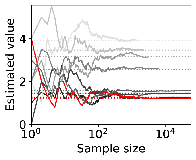
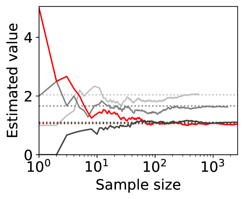
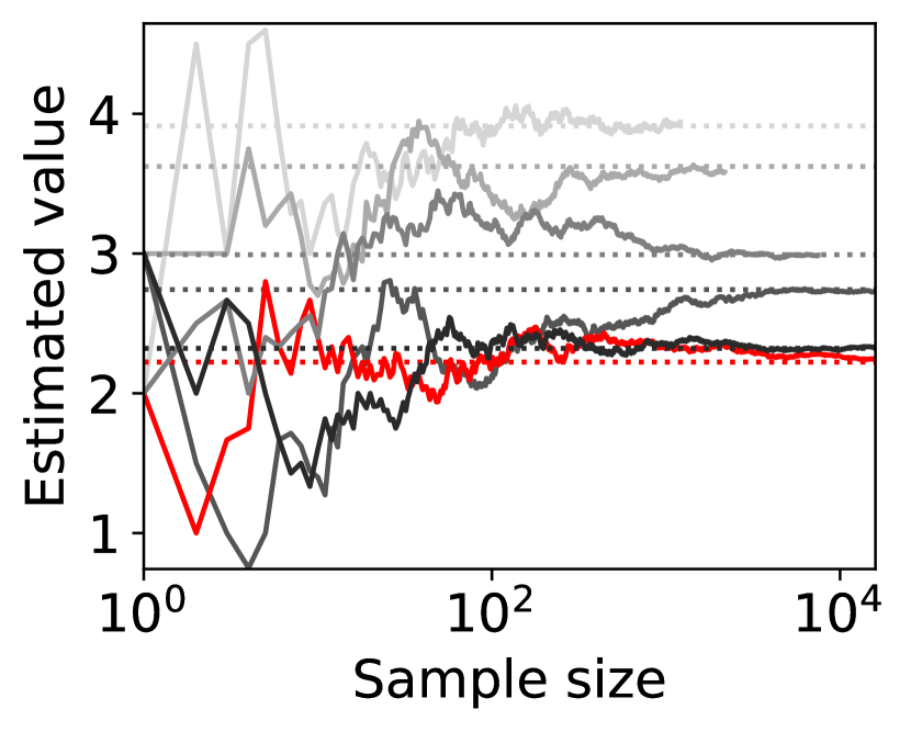
Figure 4 shows representative sample paths of the estimated values of for each when -PAC SE-BME111Minimization in Algorithm 4 is translated into maximization. is used to evaluate (i.e., (20) with ). Each panel in Figure 4 shows curves, where the red curve corresponds to the one with minimum .
Observe that the types (arms) that have close to the minimum mean, , survive until SE-BME terminates, and their means are evaluated with sufficient accuracy. On the other hand, the types that have large means are eliminated after a relatively small number of samples without being estimated precisely, which contributes to reducing the number of evaluating the value of the efficient social decision .

(a) against number of players
(b) against number of types
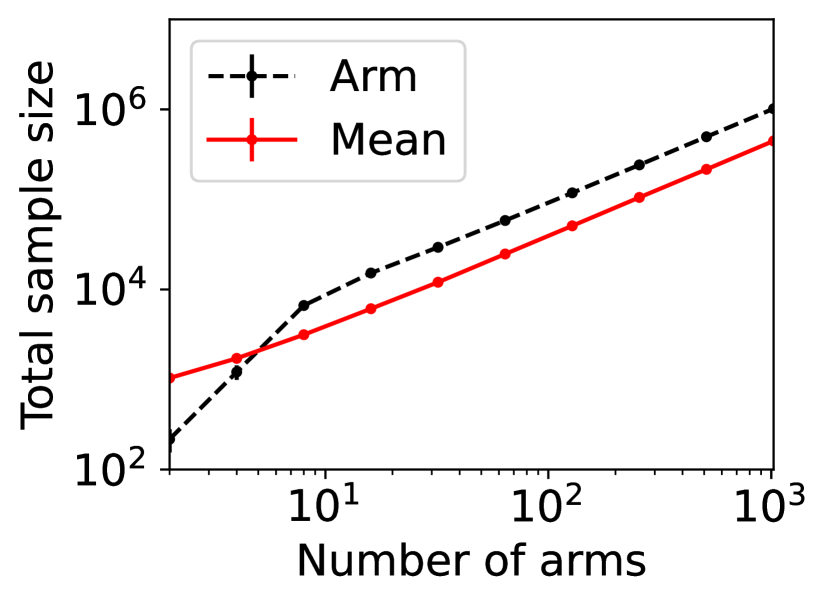
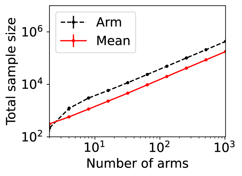
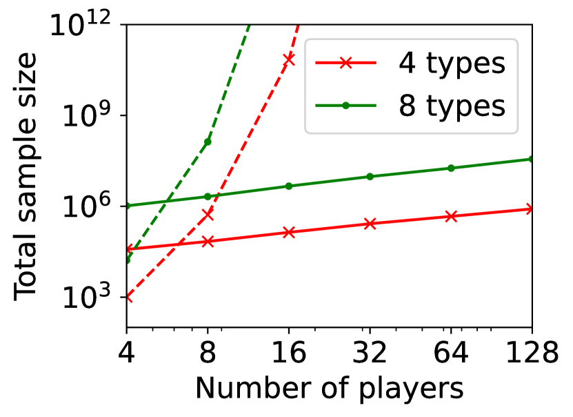
In Figure 5, we study how much SE-BME can reduce the number of evaluations of needed to estimate for all with the accuracy that is shown in Figure 4 (i.e., using the same values of and ). Recall that in the setting under consideration. Hence, the exact computation of for a single would require evaluating for different values of , but evaluations of are also sufficient to exactly compute for all , because we can cache the value of and reuse it when it is needed. Since the computational complexity associated with evaluating with (7) is the bottleneck, the unique sample size is what we should be interested in. Similar to exact computation, SE-BME also benefits from caching and reusing the values of . Figure 5 compares the unique sample size required by the exact computation and -PAC SE-BME.
Figure 5(a) implies that SE-BME (shown with solid curves) evaluates the total value of the efficient social decision, , by orders of magnitude smaller number of times than what is required by exact computation (shown with dashed curves). While the number of evaluations of grows exponentially with the number of players (specifically, ) when exact computation is used, it grows only polynomially (in fact, slightly slower than linearly) when SE-BME is used. This relative insensitivity of the sample complexity of SE-BME to the number of players makes intuitive sense, because the number of players only affects the distribution of the reward and keeps the number of arms unchanged.
Figure 5(b) shows the number of evaluations of against the number of types for any . The advantage of SE-BME over exact computation is relatively minor when we increase the number of types instead of the number of players, since increasing the number of types directly increases the number of arms. In all cases, however, we can observe that SE-BME can significantly reduce the unique sample size.
(a) against number of players
(b) against number of types
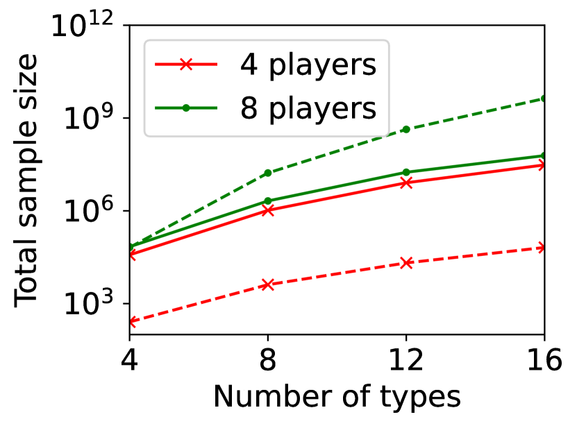
Figure 6 shows the total sample size, rather than the unique sample size, required by exact computation (dashed curves) and SE-BME (solid curves). The total sample size with exact computation is . While is evaluated times for each with exact computation, SE-BME may waste evaluating the same more often particularly when there are only a small number of players. This reduces benefits of SE-BME for total sample size, as compared to the unique sample size.
A.4.3 Individual rationality and budget balance with Best Mean Estimation
We next address the question of how well -IR and -SBB are guaranteed when we estimate with BME rather than computing it exactly. We continue to use the setting of mechanism design introduced in Section A.4.2. Recall that -IR is guaranteed when is given by (57) and (18), and -SBB is guaranteed when is given by (57) and (58). However, these are guaranteed only when the expected values, and , are exactly computed. In this section, we quantitatively evaluate how well -IR and -SBB are satisfied when those expected values are estimated from samples. Throughout this section, we study the case with and (i.e., ).

(a) players’ utility
(b) mediator’s revenue
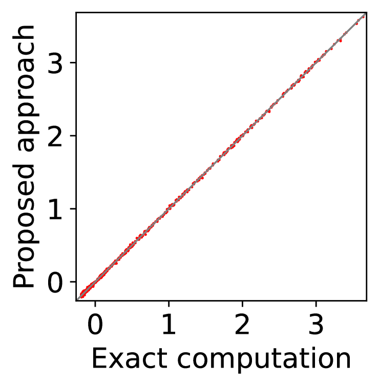
(c) player’s utility
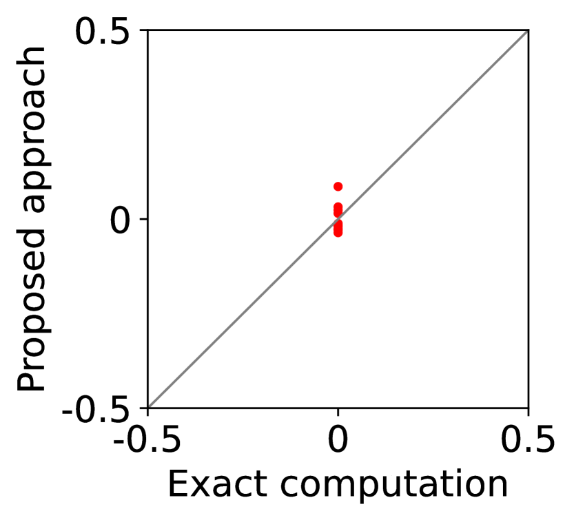
(d) mediator’s revenue
In Figure 7, we first evaluate the best mean, , either with exact computation or with BME, then compute with (57) and (18) for Columns (a)-(b) and with (57) and (58) for Columns (c)-(d), and finally evaluate the expected utility of each player (the left-hand side of (11)) for Columns (a) and (c) and the expected revenue of the mediator (the left-hand side of (12)) for Columns (b) and (d) by setting . Even if the best mean is estimated with BME, we evaluate the expectations on the left-hand side of (11) and (12) with exact computation, because these are the expected utility and the expected revenue that the players and the mediator will experience. Here, we repeat the experiment with 10 different random seeds, so that there are 10 data-points in Columns (b) and (d), and each of Columns (a) and (c) has data-points, where each data-point corresponds to a player of a particular type with a particular random seed.
Overall, Columns (a) and (c) of Figure 7 show that the expected utility experienced by the players is relatively insensitive to whether the best mean is evaluated with exact computation (horizontal axes) or with BME (vertical axes). Taking a closer look, we can observe that, in this particular setting, 0-IR is violated for some of the players in Column (c) even if the best mean is computed exactly, while it is guaranteed for any player of any type in Column (a) if the best mean is computed exactly.
On the other hand, as is shown in Columns (b) and (d), the mediator experiences non-negligible difference in its expected revenue depending on whether the best mean is evaluated with exact computation or with BME. It is to be expected that the mediator experiences relatively larger variance in its expected revenue, because (12) involves the summation , while (11) only involves for a single . In particular, it is evident in Column (d) that 0-WBB (let alone 0-SBB) is violated when the best mean is estimated with BME (vertical axes), while it is always guaranteed with exact computation (horizontal axes). In Column (b), 0-WBB is violated regardless of whether the best mean is computed exactly or with BME, since satisfying 0-WBB and 0-IR for all players (together with DE and DSIC) is impossible in this particular setting.
A simple remedy to this violation of -WBB is to replace the with a when we compute the from the best means, for , estimated with BME. By considering the ()-PAC guarantee for the error in the estimation, we can guarantee that -WBB is satisfied with high probability by setting an appropriate value of . Analogously, we may replace the with a to provide a guaranteed that -IR is satisfied with high probability when the best mean is estimated with BME. See Theorem 2.
(a) players’ utility
(b) mediator’s revenue
(c) players’ utility
(d) mediator’s revenue
As an example, we set in Figure 8. The consequence of replacing with is as expected. In Columns (b) and (d), the expected revenue of the mediator when the best mean is estimated with BME (Proposed approach) is shifted to the above by . Although it may be unclear from Columns (a) and (c), the corresponding expected utility of each player is shifted to the left by . In practice, we may choose and by taking into account these shifts as well as the condition on the feasibility of LP (Corollary 1).
(a) players’ utility
(b) mediator’s revenue
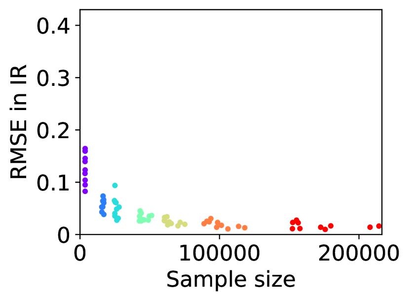
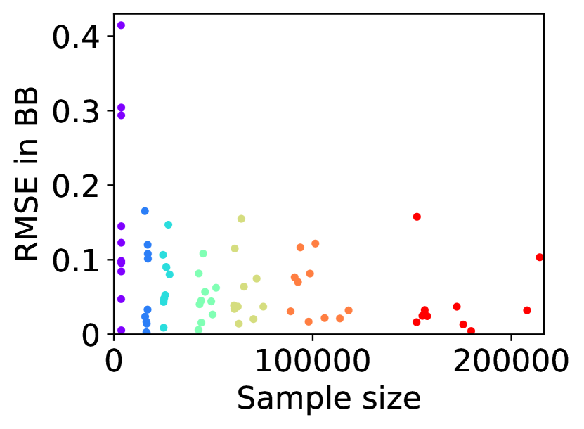
In Figure 9, we show the Root Mean Squared Error (RMSE) in the expected utility of each player (a) and the expected revenue of the mediator (b) that are estimated with BME for the case with players, each with types. Here, we fix and vary from 1.0 to 0.15 in the BME. For each pair of , the experiments are repeated 10 times with different random seeds. The total sample size increases as the value of decreases. Hence, the purple dots correspond to , and the red dots are . Overall, we can observe that RMSE can be reduced by using small at the expense of increased sample size, that relatively large values such as gives reasonably small RMSE, and that larger values of have diminishing effects on RMSE.
A.4.4 Computational requirements
We have run all of the experiments on a single core with at most 66 GB memory without GPUs in a cloud environment. The associated source code is submitted as a supplementary material and will be open-sourced upon acceptance. Table A.4.4 summarizes the CPU time and maximum memory require to generate each figure. For example, CPU time for Figure 3(a) is the time to generate three panels in Column (a) of Figure 3. Note that the CPU time and maximum memory reported in Table A.4.4 are not optimized and include time and memory for storing intermediate results and other processing for debugging purposes; these should be understood as the computational requirements to execute the source code as is.
CPU time and maximum memory required to generate figures Figure CPU Time (seconds) Max Memory (GB) Figure 3(a) 413.1 Figure 3(b) 81.9 Figure 3(c) 40.4 Figure 4(a)† 0.7 Figure 4(b)† 1.1 Figure 4(c)† 80.1 1.9 Figure 5(a) and Figure 6(a) 7,883.0 65.5 Figure 5(b) and Figure 6(b) 2,935.2 17.0 Figure 7(a)-(b) and Figure 8(a)-(b)‡ 17,531.6 1.6 Figure 7(c)-(d) and Figure 8(c)-(d)‡ 17,416.3 1.6 Figure 9 527.9
-
†
Figure 4 shows the results with one random seed, but here the CPU Time reports the average over 10 seeds, and Max Memory reports the maximum over 10 seeds.
- ‡
A.5 Details of Section 8
A.5.1 Limitations
While the proposed approach makes major advancement in the field, it certainly has limitations. Here, we discuss four major limitations of this work as well as interesting directions of research motivated by those limitations.
First, when types are not independent between players, the sufficient condition in Lemma 1 may not be necessary (Proposition 1). This means that the LP may be feasible even when the condition in the lemma is violated, and our results do not provide optimal solutions for those cases. Further research is needed to understand exactly when the sufficient condition is also necessary. It is also important to develop efficient methods for solving the LP when the types are dependent.
Second, our mechanisms guarantee strong budget balance (SBB) and individual rationality (IR) in expectation with respect to the distribution of the players’ types, but this does not guarantee that those properties are satisfied ex post (for any realization of the types). Although the satisfaction in expectation is often sufficient for risk-neutral decision makers, it is important to let the mediator and the participants aware that they may experience negative utilities even if their expected utilities are nonnegative. It would also be an interesting direction of research to extend the proposed approach towards achieving these properties ex post.
Finally, our experiments have considered environments with up to 128 players, each with at most 16 types. Although these are substantially larger than the environment studied in Osogami et al., (2023), they certainly do not cover the scale needed for all applications. While (10-100 times) larger environments could be handled with improved implementation and greater computational resources, essentially new ideas would be needed for substantially (over times) larger environments or continuous type space. It would be an interesting direction of research to identify and exploit structures of particular environments for designing scalable approaches of mechanism design for those environments.
A.5.2 Societal impacts
We expect that the proposed approach has several positive impacts on trading networks in particular and the society in general. In particular, the proposed approach enables mechanisms that can maximize the efficiency of a trading network and minimize the fees that the participants need to pay to the mediator. Also, the DSIC guaranteed by the proposed approach would make it more difficult for malicious participants to manipulate the outcome of a trading network.
On the other hand, the proposed approach might have negative impacts depending on where and how it is applied. For example, although the proposed approach guarantees individual rationality, some of the participants might get less benefits from the mechanism designed with our approach than other participants. This can happen, because maximizing the social welfare does not mean that all the participants are treated fairly. Before applying the mechanisms designed with the proposed approach, it is thus recommended to assess whether such fairness needs to be considered and to take any actions that mitigate the bias if needed.
Appendix B Proofs
B.1 Proofs on the lemmas and corollaries in Section 5
Proof of Lemma 1.
Proof of Lemma 2.
Proof of Lemma 3.
We first rewrite the LP (10)-(12) in the following equivalent form:
| (48) | ||||
| (49) | ||||
| (50) |
Then it can be easily observed that the optimal objective value must be equal to (i.e., when equality holds in (50)), since changing in a way it decreases the value of only makes (49) more satisfiable222This implies that -SBB is satisfied whenever -WBB is satisfied.
Proof of Proposition 1.
We construct an example that satisfies (11)-(12) but violates (13). Let ; ; ; . We assume that the types are completely dependent (namely, surely) and let be the probability that (hence, with probability ).
Proof of Corollary 2.
Proof of Corollary 3.
B.2 Proofs of the lemmas, theorem, and proposition in Section 6
Proof of Lemma 4.
Since the sample complexity of PAC-BAI in Step 1 is and Step 3 pulls an arm at most times, the sample complexity of Algorithm 3 is at most . Hence, it remains to prove (23).
Recall that is a random variable representing the index of the best arm returned by Algorithm 2 (PAC-BAI). Then we have the following bound:
| (68) | ||||
| (69) | ||||
| (70) | ||||
| (71) | ||||
| (72) | ||||
where the last inequality follows from PAC() of BAI.
Since is the average of samples from arm , where is the number of times Algorithm 2 (PAC-BAI) has pulled arm , we have . Hence, applying Hoeffding’s inequality to the last term of (72), we obtain
| (73) | ||||
| (74) | ||||
| (75) | ||||
| where the first inequality is obtained by applying Hoeffding’s inequality to the sample mean of independent random variables having support in , and the second inequality follows from . We can also show the following inequality in an analogous manner: | ||||
| (76) | ||||
By applying (75)-(76) to (72), we finally establish the bound to be shown:
| (77) | ||||
| by the definition of | (78) | |||
| (79) | ||||
| (80) | ||||
| (81) |
∎
Proof of Lemma 7.
Although the lemma is stated in Even-Dar et al., (2002) with reference to Chernoff, (1972), this specific lemma is neither stated nor proved explicitly in Chernoff, (1972). For completeness, here, we prove the lemma following the general methodology provided in Chernoff, (1972). Specifically, we derive the expected sample size required by the sequential probability-ratio test (SPRT; Section 10 of Chernoff, (1972)), whose optimality (Theorem 12.1 of Chernoff, (1972)) will then establish the lemma.
Consider two hypotheses, and , for the probability distribution of a random variable , which takes either the value of 1 or , where
| (82) | ||||
| (83) |
Consider the SPRT procedure that takes i.i.d. samples, , from until the stopping time when
| (84) |
hits either or . When hits , we identify as the correct hypothesis. When hits , we identify as the correct hypothesis.
Let
| (85) |
Since is a stopping time, by Wald’s lemma, we have
| (86) | ||||
| (87) | ||||
| (88) |
Let be the probability of making the error in identifying the correct hypothesis. Then we must have
| (89) | ||||
| (90) |
| (91) |
Now, notice that hits when we have
| (92) |
for the first time and hits when we have
| (93) |
for the first time. Hence, by the gambler’s ruin probability, we have
| (94) |
which implies
| (95) |
Proof of Lemma 5.
We will construct an algorithm that correctly identifies the mean of with probability at least using at most samples of in expectation given the access to an -PAC BME with sample complexity . The algorithm first draws and independently from a uniformly distribution over .
Consider two environments of -armed bandit, and , where every arm gives the reward according to the Bernoulli distribution with mean except that the reward of arm in has the same distribution as and the reward of arm in has the same distribution as . Note that the algorithm can simulate the reward with the known mean using the algorithm’s internal random number generators. Only when the algorithm pulls arm of or arm of , it uses the sample of , which contributes to the sample complexity of the algorithm.
The algorithm then runs two copies of the -PAC BME with sample complexity in parallel: one referred to as BME+ is run on , and the other referred to as BME- is run on . At each step, let be the number of samples BME+ has taken from arm by that step and be the corresponding number BME- has taken from arm . If , the algorithm lets BME+ pull an arm; otherwise, the algorithm lets BME- pull an arm. Therefore, at any step.
This process is continued until one of BME+ and BME- terminates and returns an estimate of the best mean. If BME+ terminates first, then the algorithm determines that if and that otherwise. If BME- terminates first, then the algorithm determines that if and that otherwise. Due to the -PAC property of BME+ and BME-, the algorithm correctly identifies the mean of with probability at least . Formally, if , we have
| (97) | ||||
| (98) | ||||
| (99) |
Analogously, can be shown if .
What remains to prove is the sample complexity of the algorithm. Recall that each of BME+ and BME- pulls arms at most times before it terminates due to their sample complexity. Notice that the arms in are indistinguishable when , and the arms in are indistinguishable when . Therefore, at least one of BME+ and BME- is run on the environment where the arms are indistinguishable. Since and are sampled uniformly at random from , BME (either BME+ or BME-) would take at most samples from in expectation if the arms are indistinguishable. Since , we establish that the sample complexity of the algorithm is in expectation. ∎
Proof of Lemma 6.
Note that the PAC estimators can give independent estimates, for and , such that
| (100) | ||||
| (101) |
which imply
| (102) |
Hence, with probability at least , the expected utility of player given its type (recall (8)) is
| (103) | ||||
| (104) |
where the first inequality follows from the PAC bound on and the definition of , and the last inequality follows from the original guarantee when is exactly computed, and the expected revenue of the mediator (recall (9)) is
| (105) | ||||
| (106) |
where the equality follows from the definition of , and the inequality follows from the PAC bound on . ∎
B.3 Proof of the propositions in Section 7
Proof of Proposition 5.
Let be the best mean, be the best mean estimated by Algorithm 4, and be the average of the first samples from arm . Let . Then we have
| (110) | ||||
| (111) | ||||
| (112) | ||||
| (113) | ||||
| (114) | ||||
| (115) | ||||
| (116) | ||||
∎
Proof of Proposition 6.
Let . Let be the set of the (strictly) best arms. Let be the average of the first samples from arm . Then we have
| (117) | ||||
| (118) | ||||
| (119) | ||||
| (120) | ||||
| (121) | ||||
| (122) | ||||
| (123) | ||||
∎