MelGlow: Efficient Waveform Generative Network Based on
Location-Variable Convolution
Abstract
Recent neural vocoders usually use a WaveNet-like network to capture the long-term dependencies of the waveform, but a large number of parameters are required to obtain good modeling capabilities. In this paper, an efficient network, named location-variable convolution, is proposed to model the dependencies of waveforms. Different from the use of unified convolution kernels in WaveNet to capture the dependencies of arbitrary waveforms, location-variable convolutions utilizes a kernel predictor to generate multiple sets of convolution kernels based on the mel-spectrum, where each set of convolution kernels is used to perform convolution operations on the associated waveform intervals. Combining WaveGlow and location-variable convolutions, an efficient vocoder, named MelGlow, is designed. Experiments on the LJSpeech dataset show that MelGlow achieves better performance than WaveGlow at small model sizes, which verifies the effectiveness and potential optimization space of location-variable convolutions.
Index Terms— speech synthesis, text-to-speech, neural vocoder, glow, location-variable convolution
1 Introduction
Recently, speech synthesis is playing an increasingly important role in the field of human-computer interaction. Since small changes in voice quality or latency can have a large impact on customer experience, it is necessary for speech product design to efficiently synthesize high quality speech, especially for smart speakers and dialogue robots. Currently, the general speech synthesis pipeline is composed of two components [1, 2, 3, 4, 5, 6, 7, 8, 9]: (1) a speech feature prediction model that transforms the text into time-aligned speech features, for example mel-spectrum, and (2) a neural vocoder that generates raw waveform from speech features. Our work focuses on the second model to efficiently generate speech with high quality from the mel-spectrum.
Traditional speech vocoders use digital signal processing (DSP) to reconstruct speech waveforms at very high rate, but their quality has always been limited [10, 11, 12, 13]. In recent research, neural vocoders have been widely studied. WaveNet [14], an autoregressive generative model, is proposed to synthesize high-quality speech at a high temporal resolution. WaveRNN [15] applies an efficient recurrent neural network to generate speech at 4 times faster than real-time and uses a weight pruning technique to make it deployable on mobile CPU. LPCNet [16] combines WaveRNN with linear prediction to significantly improve the efficiency of speech synthesis. Parallel WaveNet [17] and ClariNet [18] use Inverse Autoregressive Flows (IAF) [19] as the student model to distill knowledge from an autoregressive teacher WaveNet. FloWaveNet [20] and WaveGlow [21] design a flow-based network [22] to generate high-quality speech and have a very simple training process. In [23], a GAN-excited linear prediction is presented to generate waveform, where the GAN generator outputs the entire excitation signal of the linear prediction. MelGAN [24] and GAN-TTS [25] implement a Generative Adversarial Network (GAN) [26] to directly generate waveforms. Similarly, based on the GAN, Parallel WaveGAN [27] proposes a joint optimization method between the adversarial loss and multi-resolution STFT loss [28] to capture the time-frequency distributions of the realistic speech signal. These GAN-based vocoders is highly parallelisable due to the design of the efficient feed-forward generator.
The key of neural vocoder is how to model the long-term dependence of waveform based on the conditioning acoustic features. In WaveNet [14], the dilated causal convolution is used to capture the long-time dependencies of waveform. where the mel-spectrum is used as the local conditioning input and added into the gated activation unit. In [29], a pitch dependent dilated convolution is designed to improve the pitch controllability of WaveNet. Due to the superior performance of the WaveNet, the dilated convolution structure is used by many subsequent neural vocoders [27, 25, 30, 31]. Although the dilated convolution enables the model to capture the long-term dependence of the waveform, a large number of convolution kernels are required in each layer of the dilated convolution to capture different time-dependent features for achieving good performance.
In this work, we propose the location-variable convolution for the design of the waveform generation network in order to capture the long-term dependency more efficiently. In detail, a kernel predictor is designed to predict the coefficients of the convolution kernels according to the conditioning acoustic features (e.g. mel-spectrum), and different segments of the waveform use the different convolution kernels to implement the convolution operation. This convolution method is used to redesign the network structure of WaveGlow [21] so as to achieve a more efficient speech vocoder, named MelGlow. Experiments on the LJSpeech dataset [32] show that higher quality speech is acquired by MelGlow in the case of a limited number of model parameters. Meanwhile, as the mode size decreases, the rate of performance degradation of MelGlow is significantly slower than that of WaveGlow. And the main contributions of our works as follow:
-
•
A novel convolution method, named location-variable convolution, is proposed to efficiently capture the long-term dependency, where the coefficients of the convolution kernels are predicted by a kernel predictor according to the conditioning input;
-
•
A more efficient speech vocoder, named MelGlow, is designed based on location-variable convolutions, and shown to generate higher quality speech than WaveGlow when limiting the model size;
-
•
The relationship between the performance of MelGlow and the number of parameters is analyzed experimentally, which illustrates that MelGlow has great potential for optimization in the future.
2 Location-Variable Convolution
In this section, we propose the location-variable convolution to model the long-term dependency of input sequence based on the local conditioning sequence, where the coefficients of the convolution kernels change throughout the convolution process.
2.1 Motivation
Reviewing the traditional vocoder using digital signal processing (DSP) method to reconstruct speech waveforms [10, 11], one popular method is the linear prediction vocoder [10] which uses the Levinson-Durbin algorithm to calculate the linear prediction coefficients of a simple all-pole linear filter [33] according to acoustic features. The prediction process of the linear predictor is similar to the convolution process of the causal convolution, except that the coefficients of the linear predictor are calculated based on the acoustic features at different frames and the coefficients of convolution kernels in the causal convolution is the same in the whole process. Inspired by this difference, we design a novel convolution with variable convolution kernel coefficients to model the long-time dependencies of waveforms more efficiently.
2.2 Structure
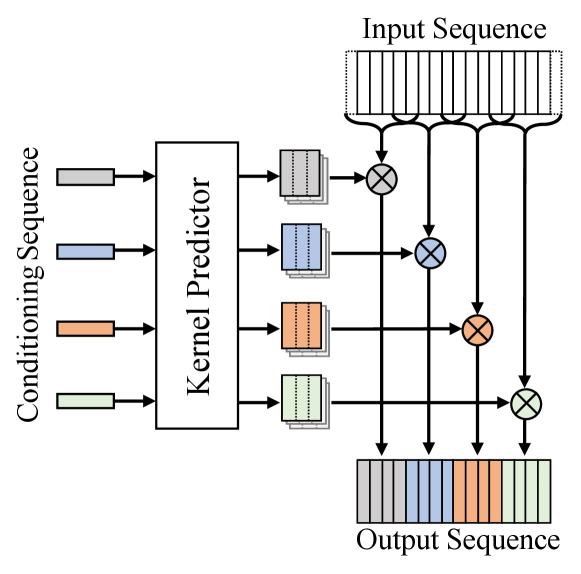
Define the input sequence to the convolution as , and define the local conditioning sequence as . An element in the local conditioning sequence is associated with a continuous interval in the input sequence. In order to model the feature of the input sequence, the location-variable convolution uses a novel convolution method, where different intervals in the input sequence use different convolution kernels to implement the convolution operation. In detail, a kernel predictor is designed to predict multiple sets of convolution kernels according to the local conditioning sequence. Each element in the local conditioning sequence corresponds to a set of convolution kernels, which is used to perform convolution operations on the associated intervals in the input sequence. And the output sequence is spliced by the convolution results on each interval.
Similar to WaveNet, the gated activation unit is also applied, and the local condition convolution can be expressed as
| (1) | ||||
| (2) | ||||
| (3) | ||||
| (4) |
where denotes the intervals of the input sequence associated with , and denote the filter and gate convolution kernels for .
For a more visual explanation, Figure 1 shows an example of the location-variable convolution, where the input sequence contains 16 elements and the conditioning sequence contains 4 elements. Each element in the conditioning sequence corresponds to 4 elements in the input sequence. Taking the conditioning sequence as input, the kernel predictor generates multiple convolution kernels, each of which is used to perform 1D convolution operation on 4 elements of the input sequence with one padding.
Note that, since location-variable convolutions can generate different kernels for different conditioning sequences, it has more powerful capability of modeling the long-term dependency than traditional convolutional network. However, the key is how to design the structure of the kernel predictor, which has a significant impact on model performance.
3 MelGlow
In this section, location-variable convolutions is used to design an efficient neural vocoder based on WaveGlow, which has fewer model parameters, but matches WaveGlow in term of speech quality.
3.1 Architecture
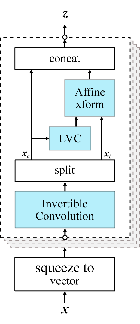
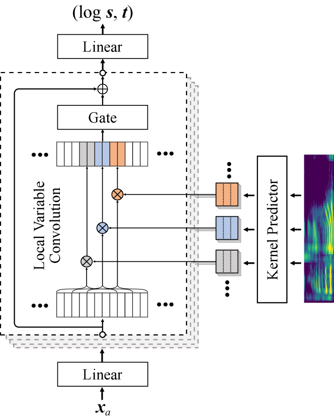
As shown Figure 2(a), we keep the main architecture of WaveGlow and use location-variable convolutions instead of the WN block. To make it easier to distinguish, the novel vocoder is called as MelGlow. The waveform data is firstly squeezed to a sequence with 8 channels, which is passed through multiple flow layers to output a latent variable. In each flow layer, the input sequence is mixed across channels by an invertible convolution, and then is split into two halves along the channel dimension. is passed through location-variable convolutions with the mel-spectrum as the conditioning sequence to produce multiplicative terms and additive terms . is scaled and translated by these terms, and then is concatenated with as the output sequence. The output sequence of the last flow layer is used to compute the log-likehood of the spherical Gaussian, which is added to the log Jacobian determinant of the invertible convolution as the final objective function, given by the log multiplicative term .
3.2 Location-Variable Convolution for MelGlow
Since the mel-spectrum is calculated from the waveform using short-time Fourier Transform (STFT) and a series of transformation operations, each element of the mel-spectrum sequence is related to a contiguous segment of samples in the waveform. Therefore, the location-variable convolution is applied based on this correlation between the mel-spectrum and waveform.
The location-variable convolution uses as the input sequence, and the mel-spectrum as the local conditioning sequence. The mel-spectrum is passed into the kernel predictor to predict multiple sets of convolution kernels, and each set of convolution kernels is used to perform convolution operations on the associated intervals of the input sequence, whose association is based on the calculation process of STFT. For example, if the Hann window size is 1024 and the hop length is 256 in STFT, each element of the mel-spectrum sequence is associated with 1024 waveform samples with 256 offsets for the next element. Due to the waveform being squeezed to a vector with 8 channels, each set of convolution kernels is used to perform dilated convolution operation on 128 elements of the input sequence with 32 offsets for next set. In addition, multiple local condition convolution layers with different dilation are stacked to expand the receptive fields, as shown in Figure 2(b).
3.3 Kernel Predictor
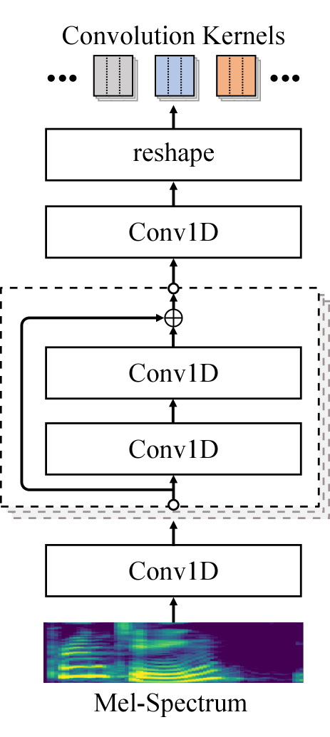
The kernel predictor is used to predict the convolution kernels according to the mel-spectrum. In our case, the kernel predictor is composed of multiple 1D convolution layers and a linear layer, as shown in Figure 2(c). The kernel size of the first 1D convolution layer is set to two without padding to adjust the alignment between the mel-spectrum sequence and the input sequence. For example, if the Hann window size is 1024 and the hop length is 256 in STFT, the waveform will be padded with 512 samples at the start and at the end, and the length of the mel-spectrum sequence is one greater than the length of the waveform divided by the hop length.
Followed by the first 1D convolution layer, multiple residual convolutional layers is applied, where each residual convolutional layer contains a 2-layer 1D convolution. The tanh activation function and the batch normalization [34] is used in each convolution layer. The linear layer is used to change the number of the channels and output the coefficients of the convolution kernels for location-variable convolutions, where the number of the output channels is determined by the number of the kernel coefficients in the location-variable convolution. Lastly, the output of the linear layer is reshaped into the form of the convolution kernel, which is used to perform location-variable convolutions on the input sequence.
4 Experiments
4.1 Training Details
4.1.1 Dataset
We train our MelGlow model on the LJSpeech dataset [32]. This dataset contains 13,100 English audio clips of a single female speaker with a total duration of approximately 24 hours. The entire dataset is randomly divided into 3 sets: 12,600 utterances for training, 400 utterances for validation, and 100 utterances for test. The sample rate of audio is set to 22,050 Hz. The mel-spectrograms are computed through a short-time Fourier transform with Hann windowing, where 1024 for FFT size, 1024 for window size and 256 for hop size. The STFT magnitude is transformed to the mel scale using 80 channel mel filter bank spanning 60 Hz to 7.6 kHz.
4.1.2 Model Configuration
In order to analyze the efficiency of the location-variable convolution, we set the configuration of MelGlow to be the same as WaveGlow on the main architecture. In detail, MelGlow has 12 flow layers and output 2 of the channels after every 4 flow layers. Each flow layer has 7 layers of location-variable convolutions with the same dilated convolution method as WaveGlow. The hidden channel of the kernel predictor is set to 64, and the number of the residual convolution layer is set to three. In addition, the channel in location-variable convolutions is set to 128, 64, 48 and 32 for comparison experiments.
We train MelGlow on a NVIDIA V100 GPU, with batch size of 8 samples. Each sample is a one-second audio clip randomly selected from the training dataset. We used the Adam optimizer [35] with a learning rate of and 600,000 iterations to train it. When training appeared to plateau, we adjusted the learning rate to . As comparative experiments, WaveGlow with different channel number (512, 256, 128 and 64) in the dilated convolution layers is chosen as baseline model, which is trained following [21].
4.2 Results
4.2.1 Vocoder Evaluation
In order to evaluate the performance of MelGlow, we use the mel-spectrograms extracted from test utterances as input to obtain synthetic audio, which is rated together with the ground truth audio (GT) by 50 native English speakers with headphones in a conventional mean opinion score (MOS) evaluation. evaluation indicator of MelGlow. At the same time, the audios generated by Griffin-Lim algorithm [12] and WaveGlow [21] are also rated together.
The evaluation results are shown in Table 1, where the number of model parameters also is illustrated. Although the best performance of MelGlow in our case does not outperform WaveGlow, MelGlow can obtain a better quality of speech at small model size. Meanwhile, as the mode size decreases, the rate of performance degradation of MelGlow is significantly slower than that of WaveGlow. According to our analysis, in the case of limited model size, MelGlow can still generate a variety of convolution kernels to capture the long-term dependent features, which enables the model to maintain good performance.
| Method | Parameters | MOS |
| GT | ||
| Griffin-Lim | ||
| WaveGlow-64 | M | |
| WaveGlow-128 | M | |
| WaveGlow-256 | M | |
| WaveGlow-512 | M | |
| MelGlow-32 | M | |
| MelGlow-48 | M | |
| MelGlow-64 | M | |
| MelGlow-128 | M |
4.2.2 Text-to-Speech Evaluation
Since speech vocoders are a component in text-to-speech systems, the vocoder and the mel-spectrum prediction network can be tested together to better evaluate the performance. In our experiments, Tacotron2 (T2) [3], FastSpeech (FS) [6] and AlignTTS (AT) [36] are used as the mel-spectrum prediction model, which predict mel-spectrograms based on the input text sequence. MelGlow with 32 channels and WaveGlow with 128 channels are used to generate waveforms based on the predicted mel-spectrums, which are rated together. As shown in Table 2, synthesized audios from MelGlow have similar quality as that from WaveGlow. This indicates that MelGlow can achieve performance that matches WaveGlow, but has fewer model parameters when limiting the model size.
4.3 Analysis of Kernel Predictor
Since MelGlow uses the kernel predictor to generate various convolution kernels for convolution operations, the design of the kernel predictor has a significant impact on the performance. We therefore analyzed the impact of the number of residual convolution layers and hidden channels in the kernel predictor. In particular, we set the number of residual convolution layers to 1, 3, 5 and the hidden channels to 32, 64 and 128 for comparison experiments. The evaluation results of these model are shown in Table 3. We can find that models of sufficient size give satisfactory performance, and more complicated networks do not achieve a significant performance improvement. One of the reasons is that the coefficients of convolution kernel predicted by the kernel predictor is not stable enough, and MelGlow is more difficult to converge if the network of the kernel predictor has too much parameters.
In WaveNet, the 1D dilated convolution is adopted to model the dependencies of waveform, where the convolution kernel is used as the waveform time feature extraction tool. In our opinion, due to the mutual independence of the acoustic features (such as mel-specturms), we can use difference convolution kernels to implement convolution operations on difference time intervals to obtain more effective feature modeling capabilities. Our exploratory experiment verified the feasibility of this approach, but the variability of the convolution kernel coefficients also affects the stability and convergence of the entire model. However, we believe that designing a more reasonable network for the kernel predictor can make MelGlow obtain better performance, and further research on the best results that the variable convolution can achieve is also our follow-up task.
| Method | MOS | Time Cost (s) |
|---|---|---|
| T2 + WaveGlow-128 | ||
| FS + WaveGlow-128 | ||
| AT + WaveGlow-128 | ||
| T2 + MelGlow-32 | ||
| FS + MelGlow-32 | ||
| AT + MelGlow-32 |
| Method | Parameters | MOS |
|---|---|---|
| MelGlow-KP-32C | ||
| MelGlow-KP-64C | ||
| MelGlow-KP-128C | ||
| MelGlow-KP-1L | ||
| MelGlow-KP-3L | ||
| MelGlow-KP-5L |
5 Conclusion
In this paper, location-variable convolutions is proposed to model the long-term dependency features of waveform according to local acoustic features, where different intervals in the input sequence use different convolution kernels to implement convolution operation. Meanwhile, it is used to design a efficient neural vocoder, named MelGlow, based on the architecture of WaveGlow. Experiments on the LJSpeech dataset show that MelGlow achieves better performance than WaveGlow in the case of limited model size due to the improved dependency capture capabilities of location-variable convolutions.
6 Acknowledgements
This paper is supported by National Key Research and Development Program of China under grant No. 2017YFB1401202, No. 2018YFB1003500 and No. 2018YFB0204400. Corresponding author is Jianzong Wang from Ping An Technology (Shenzhen) Co., Ltd.
References
- [1] Jose Sotelo, Soroush Mehri, Kundan Kumar, Joao Felipe Santos, Kyle Kastner, Aaron Courville, and Yoshua Bengio, “Char2Wav: End-to-end speech synthesis,” in ICLR Workshop, 2017.
- [2] Yuxuan Wang, RJ Skerry Ryan, Daisy Stanton, Yonghui Wu, Ron J Weiss, Navdeep Jaitly, Zongheng Yang, Ying Xiao, Zhifeng Chen, Samy Bengio, et al., “Tacotron: Towards end-to-end speech synthesis,” in Annual Conference of the International Speech Communication Association (Interspeech), 2017.
- [3] Jonathan Shen, Ruoming Pang, Ron J Weiss, Mike Schuster, Navdeep Jaitly, Zongheng Yang, Zhifeng Chen, Yu Zhang, Yuxuan Wang, Rj Skerrv-Ryan, et al., “Natural tts synthesis by conditioning wavenet on mel spectrogram predictions,” in International Conference on Acoustics, Speech and Signal Processing (ICASSP), 2018.
- [4] Naihan Li, Shujie Liu, Yanqing Liu, Sheng Zhao, Ming Liu, and M Zhou, “Neural speech synthesis with transformer network,” in AAAI Conference on Artificial Intelligence (AAAI), 2019.
- [5] Wei Ping, Kainan Peng, Andrew Gibiansky, Sercan O Arik, Ajay Kannan, Sharan Narang, Jonathan Raiman, and John Miller, “Deep Voice 3: 2000-speaker neural text-to-speech,” in International Conference on Learning Representations (ICLR), 2018.
- [6] Yi Ren, Yangjun Ruan, Xu Tan, Tao Qin, Sheng Zhao, Zhou Zhao, and Tie-Yan Liu, “FastSpeech: Fast, robust and controllable text to speech,” in Advances in Neural Information Processing Systems (NIPS), 2019.
- [7] Kainan Peng, Wei Ping, Zhao Song, and Kexin Zhao, “Non-autoregressive neural text-to-speech,” in International Conference on Machine Learning (ICML), 2019.
- [8] Takuma Okamoto, Tomoki Toda, Yoshinori Shiga, and Hisashi Kawai, “Real-time neural text-to-speech with sequence-to-sequence acoustic model and WaveGlow or single gaussian WaveRNN vocoders,” in Annual Conference of the International Speech Communication Association (Interspeech), 2019.
- [9] Zhen Zeng, Jianzong Wang, Ning Cheng, Tian Xia, and Jing Xiao, “Prosody learning mechanism for speech synthesis system without text length limit,” in Annual Conference of the International Speech Communication Association (Interspeech), 2020.
- [10] Bishnu S Atal and Suzanne L Hanauer, “Speech analysis and synthesis by linear prediction of the speech wave,” The Journal of The Acoustical Society of America, vol. 50, no. 2B, pp. 637–655, 1971.
- [11] J Markel and A Gray, “A linear prediction vocoder simulation based upon the autocorrelation method,” IEEE Transactions on Acoustics, Speech, and Signal Processing, vol. 22, no. 2, pp. 124–134, 1974.
- [12] Daniel Griffin and Jae Lim, “Signal estimation from modified short-time fourier transform,” IEEE Transactions on Acoustics, Speech, and Signal Processing, vol. 32, no. 2, pp. 236–243, 1984.
- [13] Masanori Morise, Fumiya Yokomori, and Kenji Ozawa, “WORLD: a vocoder-based high-quality speech synthesis system for real-time applications,” IEICE Transactions on Information and Systems, vol. 99, no. 7, pp. 1877–1884, 2016.
- [14] Aäron van den Oord, Sander Dieleman, Heiga Zen, Karen Simonyan, Oriol Vinyals, Alex Graves, Nal Kalchbrenner, Andrew Senior, and Koray Kavukcuoglu, “WaveNet: A generative model for raw audio,” arXiv preprint arXiv:1609.03499, 2016.
- [15] Nal Kalchbrenner, Erich Elsen, Karen Simonyan, Seb Noury, Norman Casagrande, Edward Lockhart, Florian Stimberg, Aaron van den Oord, Sander Dieleman, and Koray Kavukcuoglu, “Efficient neural audio synthesis,” in International Conference on Machine Learning (ICML), 2018.
- [16] Jean Marc Valin and Jan Skoglund, “LPCNet: Improving neural speech synthesis through linear prediction,” in International conference on Acoustics, Speech and Signal Processing (ICASSP). IEEE, 2019.
- [17] Aaron van den Oord, Yazhe Li, Igor Babuschkin, Karen Simonyan, Oriol Vinyals, Koray Kavukcuoglu, George van den Driessche, Edward Lockhart, Luis Cobo, Florian Stimberg, Norman Casagrande, Dominik Grewe, Seb Noury, Sander Dieleman, Erich Elsen, Nal Kalchbrenner, Heiga Zen, Alex Graves, Helen King, Tom Walters, Dan Belov, and Demis Hassabis, “Parallel WaveNet: Fast high-fidelity speech synthesis,” in International Conference on Machine Learning (ICML), 2018.
- [18] Wei Ping, Kainan Peng, and Jitong Chen, “ClariNet: Parallel wave generation in end-to-end text-to-speech,” in International Conference on Learning Representations (ICLR), 2018.
- [19] Durk P Kingma, Tim Salimans, Rafal Jozefowicz, Xi Chen, Ilya Sutskever, and Max Welling, “Improved variational inference with inverse autoregressive flow,” in Advances in Neural Information Processing Systems (NIPS). 2016.
- [20] Sungwon Kim, Sang-Gil Lee, Jongyoon Song, Jaehyeon Kim, and Sungroh Yoon, “FloWaveNet : A generative flow for raw audio,” in International Conference on Machine Learning (ICML), 2019.
- [21] Ryan Prenger, Rafael Valle, and Bryan Catanzaro, “WaveGlow: A flow-based generative network for speech synthesis,” in International Conference on Acoustics, Speech and Signal Processing (ICASSP), 2019.
- [22] Danilo Jimenez Rezende and Shakir Mohamed, “Variational inference with normalizing flows,” in International Conference on Machine Learning (ICML), 2015.
- [23] Lauri Juvela, Bajibabu Bollepalli, Junichi Yamagishi, and Paavo Alku, “GELP: Gan-excited linear prediction for speech synthesis from mel-spectrogram,” in Annual Conference of the International Speech Communication Association (Interspeech), 2019.
- [24] Kundan Kumar, Rithesh Kumar, Thibault de Boissiere, Lucas Gestin, Wei Zhen Teoh, Jose Sotelo, Alexandre de Brébisson, Yoshua Bengio, and Aaron C Courville, “MelGAN: Generative adversarial networks for conditional waveform synthesis,” in Advances in Neural Information Processing Systems (NIPS). 2019.
- [25] Mikoaj Bińkowski, Jeff Donahue, Sander Dieleman, Aidan Clark, Erich Elsen, Norman Casagrande, Luis C Cobo, and Karen Simonyan, “High fidelity speech synthesis with adversarial networks,” in International Conference on Learning Representations (ICLR), 2020.
- [26] Ian Goodfellow, Jean Pouget-Abadie, Mehdi Mirza, Bing Xu, David Warde-Farley, Sherjil Ozair, Aaron Courville, and Yoshua Bengio, “Generative adversarial nets,” in Advances in Neural Information Processing Systems (NIPS), 2014.
- [27] R. Yamamoto, E. Song, and J. Kim, “Parallel WaveGan: A fast waveform generation model based on generative adversarial networks with multi-resolution spectrogram,” in International conference on Acoustics, Speech and Signal Processing (ICASSP), 2020.
- [28] Sercan Omer Arik, Heewoo Jun, and Gregory Diamos, “Fast spectrogram inversion using multi-head convolutional neural networks,” IEEE Signal Processing Letters, vol. PP, pp. 1–1, 2018.
- [29] Yi-Chiao Wu, Tomoki Hayashi, Patrick Lumban Tobing, Kazuhiro Kobayashi, and Tomoki Toda, “Quasi-Periodic WaveNet Vocoder: A pitch dependent dilated convolution model for parametric speech generation,” .
- [30] P. L. Tobing, Y. Wu, T. Hayashi, K. Kobayashi, and T. Toda, “Efficient shallow wavenet vocoder using multiple samples output based on laplacian distribution and linear prediction,” in International Conference on Acoustics, Speech and Signal Processing (ICASSP), 2020.
- [31] N. Wu and Z. Ling, “WaveFFJORD: Ffjord-based vocoder for statistical parametric speech synthesis,” in International Conference on Acoustics, Speech and Signal Processing (ICASSP), 2020.
- [32] Keith Ito, “The LJ Speech dataset,” https://keithito.com/ LJ-Speech-Dataset/, 2017.
- [33] John Makhoul, “Linear prediction: A tutorial review,” Proceedings of the IEEE, vol. 63, no. 4, pp. 561–580, 1975.
- [34] Sergey Ioffe and Christian Szegedy, “Batch normalization: Accelerating deep network training by reducing internal covariate shift,” in International Conference on Machine Learning (ICML), 2015.
- [35] Diederik P. Kingma and Jimmy Ba, “Adam: A method for stochastic optimization,” in International Conference on Learning Representations (ICLR), 2015.
- [36] Zhen Zeng, Jianzong Wang, Ning Cheng, Tian Xia, and Jing Xiao, “AlignTTS: Efficient feed-foward text-to-speech system without explicit alignment,” in International Conference on Acoustics, Speech and Signal Processing (ICASSP), 2020.