Memory capacity of neural networks with threshold and ReLU activations
Abstract.
Overwhelming theoretical and empirical evidence shows that mildly overparametrized neural networks – those with more connections than the size of the training data – are often able to memorize the training data with accuracy. This was rigorously proved for networks with sigmoid activation functions [23, 13] and, very recently, for ReLU activations [24]. Addressing a 1988 open question of Baum [6], we prove that this phenomenon holds for general multilayered perceptrons, i.e. neural networks with threshold activation functions, or with any mix of threshold and ReLU activations. Our construction is probabilistic and exploits sparsity.
1. Introduction
This paper continues the long study of the memory capacity of neural architectures. How much information can a human brain learn? What are fundamental memory limitations, and how should the “optimal brain” be organized to achieve maximal capacity? These questions are complicated by the fact that we do not sufficiently understand the architecture of the human brain. But suppose that a neural architecture is known to us. Consider, for example, a given artificial neural network. Is there a general formula that expresses the memory capacity in terms of the network’s architecture?
1.1. Neural architectures
In this paper we study a general layered, feedforward, fully connected neural architecture with arbitrarily many layers, arbitrarily many nodes in each layer, with either threshold or ReLU activation functions between all layers, and with the threshold activation function at the output node.
Readers unfamiliar with this terminology may think of a neural architecture as a computational device that can compute certain compositions of linear and nonlinear maps. Let us describe precisely the functions computable by a neural architecture. Some of the best studied and most popular nonlinear functions , or “activation functions”, include the threshold function and the rectified linear unit (ReLU), defined by
| (1.1) |
respectively.111It should be possible to extend out results for other activation functions. To keep the argument simple, we shall focus on the threshold and ReLU nonlinearities in this paper. We call a map pseudolinear if it is a composition of an affine transformation and a nonlinear transformation applied coordinate-wise. Thus, is pseudolinear map if it can be expressed as
where is a matrix of “weights”, is a vector of “biases”, and is either the threshold or ReLU function (1.1), which we apply to each coordinate of the vector .
A neural architecture computes compositions of pseudolinear maps, i.e. functions of the type
where , , …, , are pseudolinear maps. Each of maps may be defined using either the threshold or ReLU function, and mix and match is allowed. However, for the purpose of this paper, we require the output function to have the threshold activation.222General neural architectures used by practitioners and considered in the literature may have more than one output node and have other activation functions at the output node.
We regard the matrices and in the definition of each pseudolinear map as free parameters of the given neural architecture. Varying these free parameters one can make a given neural architecture compute different functions . Let us denote the class of such functions computable by a given architecture by
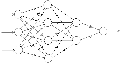
A neural architecture can be visualized as a directed graph, which consists of layers each having nodes (or neurons), and one output node. Successive layers are connected by bipartite graphs, each of which represents a pseudolinear map . Each neuron is a little computational device. It sums all inputs from the neurons in the previous layer with certain weights, applies the activation function to the sum, and passes the output to neurons in the next layer. More specifically, the neuron determines if the sum of incoming signals from the previous layers exceeds a certain firing threshold . If so, the neuron fires with either a signal of strength (if is the threshold activation function) or with strength proportional to the incoming signal (if is the ReLU activation).
1.2. Memory capacity
When can a given neural architecture remember a given data? Suppose, for example, that we have digital pictures of cats and dogs, encoded as as vectors , and labels where stands for a cat and for a dog. Can we train a given neural architecture to memorize which images are cats and which are dogs? Equivalently, does there exist a function such that
| (1.2) |
A common belief is that this should happen for any sufficiently overparametrized network – an architecture that that has significantly more free parameters than the size of the training data. The free parameters of our neural architecture are the weight matrices and the bias vectors . The number of biases is negligible compared to the number of weights, and the number of free parameters is approximately the same as the number of connections333We dropped the number of output connections, which is negligible compared to .
Thus, one can wonder whether a general neural architecture is able to memorize the data as long as the number of connections is bigger than the size of the data, i.e. as long as
| (1.3) |
Motivated by this question, one can define memory capacity of a given architecture as the largest size of general data the architecture is able to memorize. In other words, the memory capacity is the largest such that for a general444One may sometimes wish to exclude some kinds of pathological data, so natural assumptions can be placed on the set of data points . In this paper, for example, we consider unit and separated points . set of points and for any labels there exists a function that satisfies (1.2).
The memory capacity is clearly bounded above by the vc-dimension,555This is because the vc-dimension is the maximal for which there exist points so that for any labels there exists a function that satisfies (1.2). The memory capacity requires any general set of points to succeed as above. which is for neural architectures with threshold activation functions [7] and for neural architectures with ReLU activation functions [5]. Thus, our question is whether these bounds are tight – is memory capacity (approximately) proportional to ?
1.3. The history of the problem
A version of this question was raised by Baum [6] in 1988. Building on the earlier work of Cover [8], Baum studied the memory capacity of multilayer perceptrons, i.e. feedforward neural architectures with threshold activation functions. He first looked at the network architecture with one hidden layer consisting of nodes (and, as notation suggests, nodes in the hidden layer and one output node). Baum noticed that for data points in general position in , the memory capacity of the architecture is about , i.e. it is proportional to the number of connections. This is not difficult: general position guarantees that the hyperplane spanned by any subset of data points misses any other data points; this allows one to train each of the neurons in the hidden layer on its own batch of data points.
Baum then asked if the same phenomenon persists for deeper neural networks. He asked whether for large there exists a deep neural architecture with a total of neurons in the hidden layers and with memory capacity at least . Such result would demonstrate the benefit of depth. Indeed, we just saw that shallow architecture has capacity just , which would be smaller than the hypothetical capacity of deeper architectures for .
There was no significant progress on Baum’s problem. As Mitchison and Durbin noted in 1989, “one significant difference between a single threshold unit and a multilayer network is that, in the latter case, the capacity can vary between sets of input vectors, even when the vectors are in general position” [17]. Attempting to count different functions that a deep network can realize on a given data set , Kowalczyk writes in 1997: “One of the complications arising here is that in contrast to the single neuron case even for perceptrons with two hidden units, the number of implementable dichotomies may be different for various -tuples in general position… Extension of this result to the multilayer case is still an open problem” [15].
The memory capacity problem is more tractable for neural architectures in which the threshold activation is replaced by one of its continuous proxies such as ReLU, sigmoid, tanh, or polynomial activation functions. Such activations allow neurons to fire with variable, controllable amplitudes. Heuristically, this ability makes it possible to encode the training data very compactly into the firing amplitudes.
Yamasaki claimed without proof in 1993 that for the sigmoid activation and for data in general position, the memory capacity of a general deep neural architecture is lower bounded , the number of connections [23]. A version of Yamasaki’s claim was proved in 2003 by Huang for arbitrary data and neural architectures with two hidden layers [13].
In 2016, Zhang et al. [25] gave a construction of an arbitrarily large (but not fully connected) neural architecture with ReLU activations and whose memory capacity is proportional to both the number of connections and the number of nodes. Hardt and Ma [12] gave a different construction of a residual network with similar properties.
1.4. Main result
Meanwhile, the original problem of Baum [6] – determine memory capacity of networks with threshold activations – has remained open. In contrast to the neurons with continuous activation functions, neurons with threshold activations either not fire at all of fire with the same unit amplitude. The strength of the incoming signal is lost when transmitted through such neurons, and it is not clear how the data can be encoded.
This is what makes Baum’s question hard. In this paper, we (almost) give a positive answer to this question.
Why “almost”? First, the size of the input layer should not affect the capacity bound and should be excluded from the count of the free parameters . To see this, consider, for example, the data points all laying on one line; with respect to such data, the network is equivalent to one with . Next, ultra-narrow bottlenecks should be excluded at least for the threshold nonlinearity: for example, any layer with just node make the number of connections that occur in the further layers irrelevant as free parameters.
In our actual result, we make somewhat stronger assumptions: in counting connections, we exclude not only the first layer but also the second; we rule out all exponentially narrow bottlenecks (not just of size one); we assume that the data points are unit and separated; finally, we allow logarithmic factors.
Theorem 1.1.
Let be positive integers, and set and . Consider unit vectors that satisfy
| (1.4) |
Consider any labels . Assume that the number of deep connections satisfies
| (1.5) |
as well as and . Then the network can memorize the label assignment exactly, i.e. there exists a map such that
| (1.6) |
Here and denote certain positive absolute constants.
In short, Theorem 1.1 states that the memory capacity of a general neural architecture with threshold or ReLU activations (or a mix thereof) is lower bounded by the number of the deep connections. This bound is independent of the depth, bottlenecks (up to exponentially narrow), or any other architectural details.
1.5. Should the data be separated?
One can wonder about the necessity of the separation assumption (1.4). Can we just assume that are distinct? While this is true for ReLU and tanh activations [24], it is false for threshold activations. A moment’s thought reveals that any pseudolinear map from to transforms any line into a finite set such of cardinality . Thus, by pigeonhole principle, any map from layer to layer is non-injective on the set of data points – which makes it impossible to memorize some label assignments – unless . In other words, if we just assume that the data points are distinct, the network must have at least as many nodes in the second layer as the number of data points. Still, the separation assumption (5.2) does not look tight and might be weakened.
1.6. Related notions of capacity
Instead of requiring the network to memorize the training data with accuracy as in Theorem 1.1, one can ask to memorize just fraction, or just a half of the training data correctly. This corresponds to a relaxed, or fractional memory capacity of neural architectures that was introduced by Cover in 1965 [8] and studied extensively afterwards.
To estimate fractional capacity of a given architecture, one needs to count all functions this architecture can realize on a given finite set points . When this set is the Boolean cube , this amounts to counting all Boolean functions the architecture can realize. The binary logarithm of the number of all such Boolean functions was called (expressive) capacity by Baldi and the author [3, 4]. For a neural architecture with all threshold activations and layers, the expressive capacity is equivalent to the cubic polynomial in the sizes of layers :
up to an absolute constant factor [4]. The factor quantifies the effect of any bottlenecks that occur before layer .
Similar results can be proved for the restricted expressive capacity where we count the functions the architecture can realize on a given finite set of points [4, Section 10.5]. Ideally, one might hope to find that all functions can be realized on a general -element set, which would imply that the memory capacity is at least . However, the current results on restricted expressive capacity are not tight enough to reach such conclusions.
2. The method
Our construction of the function in Theorem 1.1 is probabilistic. Let us first illustrate our approach for the architecture with two hidden layers, and with threshold activations throughout. We would like to find a composition of pseudolinear functions
that fits the given data as in (1.6).
The first two maps and are enrichment maps whose only purpose is spread the data in the space, transforming it into an almost orthogonal set. Specifically, will transform the separated points into -orthogonal points (Theorem 5.2), will transform the -orthogonal points into -orthogonal points (Theorem 5.4), and, finally, the perception map will fit the data: .
2.1. Enrichment
Our construction of the enrichment maps and exploits sparsity. Both maps will have the form
where is an Gaussian random matrix with all i.i.d. coordinates, are independent standard normal random vectors, is the vector whose all coordinates equal some value .
If is large, is a sparse random vector with i.i.d. Bernoulli coordinates. A key heuristic is that independent sparse random vectors are almost orthogonal. Indeed, if and are independent random vectors in whose all coordinates are Bernoulli(p), then while , so we should expect
making and almost orthogonal for small .
Unfortunately, the sparse random vectors and are not independent unless and are exactly orthogonal. Nevertheless, our heuristic that sparsity induces orthogonality still works in this setting. To see this, let us check that the correlation of the coefficients and is small even if and are far from being orthogonal. A standard asymptotic analysis of the tails of the normal distribution implies that
| (2.1) |
if and are unit and -separated (Proposition 3.1), and
| (2.2) |
if and are unit and -orthogonal (Proposition 3.2).
Now we choose so that the coordinates of and are sparse enough, i.e.
thus . Choose sufficiently small to make the factor in (2.2) nearly constant, i.e.
Finally, we choose the separation threshold sufficiently large to make the factor in (2.1) less than , i.e.
this explains the form of separation condition in Theorem 1.1.
2.2. Perception
As we just saw, the enrichment process transforms our data points into -orthogonal vectors . Let us now find a perception map that can fit the labels to the data: .
Consider the random vector
where the signs are independently chosen with probability each. Then, separating the -th term from the sum defining and assuming for simplicity that are unit vectors, we get
Taking the expectation over independent signs, we see that
where and by almost orthogonality. Hence
if . This yields , or
Since , the “mirror perceptron”666The mirror perceptron requires not one but two neurons to implement, which is not a problem for us.
fits the data exactly: .
2.3. Deeper networks
The same argument can be repeated for networks with variable sizes of layers, i.e. . Interestingly, the enrichment works fine even if , making the lower-dimensional data almost orthogonal even in very high dimensions. This explains why (moderate) bottlenecks – narrow layers – do not restrict memory capacity.
The argument we outlined allows the network to fit around data points, which is not very surprising, since we expect the memory capacity be proportional to the number of connections and not the number of nodes. However, the power of enrichment allows us to boost the capacity using the standard method of batch learning (or distributed learning).
Let us show, for example, how the network with three hidden layers can fit data points . Partition the data into batches each having data points. Use our previous result to train each of the neurons in the fourth layer on its own batch of points, while zeroing out all labels outside that batch. Then simply sum up the results. (The details are found in Theorem 7.1.)
This result can be extended to deeper networks using stacking, or unrolling a shallow architecture into a deep architecture, thereby trading width for depth. Figure 2 gives an illustration of stacking, and Theorem 7.2 provides the details. A similar stacking construction was employed in [4].
The success of stacking indicates that depth has no benefit formemorization purposes: a shallow architecture can memorize roughly as much data as any deep architecture with the same number of connections. It should be noted, however, that training algorithms commonly used by practitioners, i.e. variants of stochastic gradient descent, do not seem to lead to anything similar to stacking; this leaves the question of benefit of depth open.
2.4. Neural networks as preconditioners
As we explained in Section 2.1, the first two hidden layers of the network act as preconditioners: they transform the input vectors into vectors that are almost orthogonal. Almost orthogonality facilitates memorization process in the deeper layers, as we saw in Section 2.2.
The idea to keep the data well-conditioned as it passes through the network is not new. The learning rate of the stochastic gradient descent (which we are not dealing with here) is related to how well conditioned is the so-called gradient Gram matrix . In the simplest scenario where the activation is ReLU and the network has one hidden layer of infinite size, is a matrix with entries
Much effort was made recently to prove that is well-conditioned, i.e. its smallest singular value of is bounded away from zero, since this can be used to establishes a good convergence rate for the stochastic gradient descent, see the papers cited in Section 1.3 and especially [1, 10, 9, panigrahi2019effect]. However, existing results that prove that is well conditioned only hold for very overparametrized networks, requiring at least nodes in the hidden layer [panigrahi2019effect]. This is a much stronger overparametrization requirement than in our Theorem 1.1.
On the other hand, as opposed to many of the results quoted above, Theorem 1.1 does not shed any light on the behavior of stochastic gradient descent, the most popular method for training deep networks. Instead of training the weights, we explicitly compute them from the data. This allows us to avoid dealing with the gradient Gram matrix: our enrichment method provides an explicit way to make the data well conditioned. This is achieved by setting the biases high enough to enforce sparsity. It would be interesting to see if similar preconditioning guarantees can be achieved with small (or even zero) biases and thus without exploiting sparsity.
A different form of enrichment was developed recently in the paper [4] which showed that a neural network can compute a lot of different Boolean functions. Toward this goal, an enrichment map was implemented in the first hidden layer. The objective of this map is to transform the input set (the Boolean cube ) into a set on which there are lots of different threshold functions – so that the next layers can automatically compute lots of different Boolean functions. While the general goal of this enrichment map in [4] is the same as in the present paper – achieve a more robust data representation that is passed to deeper layers – the constructions of these two enrichment maps are quite different.
2.5. Further observations and questions
As we saw in the previous section, we utilized the first two hidden layers of the network to preprocess, or enrich, the data vectors . This made us skip the sizes of the first two layers when we counted the number of connections . If these vectors are already nice, no enrichment may be necessary, and we have a higher memory capacity.
Suppose, for example, that the data vectors in Theorem 1.1 are -orthogonal. Then, since no enrichment is needed in this case, the conclusion of the theorem holds with
which is the sum of all connections in the network.
If, on the other hand, the data vectors in Theorem 1.1 are only -orthogonal, just the second enrichment is needed, and so the conclusion of the theorem holds with
which is the sum of all connections between the non-input layers.
This make us wonder: can enrichment be always achieved in one step instead of two? Can one find a pseudolinear map that transforms a given set of -separated vectors (say, for ) into a set of -orthogonal vectors? If this is possible, we would not need to exclude the second layer from the parameter count, and Theorem 1.1 would hold for .
A related question for further study is to find an optimal separation threshold in the assumption in Theorem 1.1, and to remove the assumption that be unit vectors. Both the logarithmic separation level of and the normalization requirement could be artifacts of the enrichment scheme we used.
There are several ways Theorem 1.1 could be extended. It should not be too difficult, for example, to allow the output layer have more than one node; such multi-output networks are used in classification problems with multiple classes.
Finally, it should be possible to extend the analysis for completely general activation functions. Threshold activations we treated are conceptually the hardest case, since they act as extreme quantizers that restrict the flow of information through the network in the most dramatic way.
2.6. The rest of the paper
In Section 3 we prove bounds (2.1) and (2.2) which control , the correlation of the coefficients of the coordinates of and . This immediately controls the expected inner product . In Section 4 we develop a deviation inequality to make sure that the inner product is close to its expectation with high probability. In Section 5, we take a union bound over all data points and thus control all inner products simultaneously. This demonstrates how enrichment maps make the data almost orthogonal – the property we outlined in Section 2.1. In Section 6, we construct a random perception map as we outlined in Section 2.2. We combine enrichment and perception in Section 7 as we outlined in Section 2.3. We first prove a version of our main result for networks with three hidden layers (Theorem 7.1); then we stack shallow networks into an arbitrarily deep architecture proving a full version of our main result in Theorem 7.2.
In the rest of the paper, positive absolute constants will be denoted , etc. The notation means that for some absolute constant and for all values of parameter . Similarly, means that where is another positive absolute constant.
We call a map almost pseudolinear if for some nonnegative constant and some pseudolinear map . For the ReLU nonlinearity, almost pseudolinear maps are automatically pseudolinear, but for the threshold nonlinearity this is not necessarily the case.
3. Correlation decay
Let and consider the random process
| (3.1) |
which is indexed by points on the unit Euclidean sphere in . Here can be either the threshold of ReLU nonlinearity as in (1.1), and is a fixed value. Due to rotation invariance, the correlation of and only depends on the distance between and . Although it seems to be difficult to compute this dependence exactly, we will demonstrate that the correlation of and decays rapidly in . We will prove this in two extreme regimes – where and are just a little separated, and where and are almost orthogonal.
3.1. Correlation for separated vectors
Cauchy-Schwarz inequality gives a trivial bound
with equality when . Our first result shows that if the vectors and are -separated, this bound can be dramatically improved, and we have
Proposition 3.1 (Correlation for separated vectors).
Consider a pair of unit vectors , and let be a number that is larger than a certain absolute constant. Then
where and .
Proof.
Step 1. Orthogonal decomposition. Consider the vectors
Then and are orthogonal and , . We claim that
| (3.2) |
To check this claim, note that if both and are greater than so is . Expressing this implication as
| (3.3) |
we conclude that (3.2) holds for the threshold nonlinearity .
To prove (3.2) for the ReLU nonlinearity, note that
Combine this bound with (3.3) to get
This yields (3.2) for the ReLU nonlinearity .
3.2. Correlation for almost orthogonal vectors
We continue to study the covariance structure of the random process . If and are orthogonal, and are independent and we have
In this subsection, we show the stability of this equality. The result below implies that if and are almost orthogonal, namely , then
Proposition 3.2 (Correlation for -orthogonal vectors).
Consider a pair of vectors satisfying
for some . Let be a number that is larger than a certain absolute constant. Then
where and .
In order to prove this proposition, we first establish a more general stability property:
Lemma 3.3.
Let and let , , , and be as in Proposition 3.2. Then, for any measurable function we have
Proof.
Consider the matrix whose rows are and , and define the function
Since the vector has coordinates and , we have . Thus
| (3.6) |
where
The assumptions on then give
| (3.7) |
Indeed, the first bound is straightforward. To verify the second bound, note that each entry of the matrix is bounded in absolute value by . Thus, the operator norm of is bounded by , which we can write as in the positive-semidefinite order. This implies that , and multiplying both sides of this relation by and , we get the second bound in (3.7).
Proof of Proposition 3.2.
By assumption, , so
| (3.8) |
where the last inequality follows by monotonicity; see Lemma A.3 for justification. Now we use the stability property of the normal distribution that we state in Lemma A.2. For larger than a suitable absolute constant and , it gives for both threshold of ReLU nonlinearities the following:
where the last bound follows since . Combining this with (3.8), we obtain the first conclusion of the lemma.
Next, Lemma 3.3 gives
| (3.9) |
Now we again use the stability property of the normal distribution, Lemma A.2, this time for . It gives for both threshold of ReLU nonlinearities the following:
Combining this with (3.9) gives
where the last step follows since . This completes the proof of Proposition 3.2. ∎
4. Deviation
In the previous section, we studied the covariance of the random process
where is either the threshold of ReLU nonlinearity as in (1.1), is a standard normal random variable, and is a fixed value. Consider a multivariate version of this process, a random pseudolinear map whose components are independent copies of . In other words, define
where are independent standard normal random vectors.
We are interested in how the map transforms the distances between different points. Since
the bounds on we proved in the previous section describe the behavior of in expectation. In this section, we use standard concentration inequalities to ensure a similar behavior with high probability.
Lemma 4.1 (Deviation).
Consider a pair of vectors such that , , and let be a number that is larger than a certain absolute constant. Define
| (4.1) |
Then for every , with probability at least we have
Proof.
Step 1. Decomposition and truncation. By construction, . The deviation from the mean is
| (4.2) |
where and . These two normal random variables are possibly correlated, and each has zero mean and variance bounded by .
We will control the sum of i.i.d. random variables in (4.2) using Bernstein’s concentration inequality. In order to apply it, we first perform a standard truncation of the terms of the sum. The level of truncation will be
| (4.3) |
where is a sufficiently large absolute constant. Consider the random variables
Then we can decompose the sum in (4.2) as follows:
| (4.4) |
Step 2. The residual is small. Let us first control the residual, i.e. the second sum on the right side of (4.4). For a fixed , the probability that is nonzero can be bounded by
| (4.5) |
where . In the second inequality, we used that and are normal with mean zero and variance at most . The third inequality follows from the asymptotic (A.2) on the tail of the normal distribution and our choice (4.3) of the truncation level with sufficiently large .
Taking the union bound we see that all vanish simultaneously with probability at least . Furthermore, by monotonicity,
| (4.6) |
where in the last step we used generalized Hölder’s inequality. Now, for the threshold nonlinearity , the terms and obviously equal , and for the ReLU nonlinearity these terms are bounded by the fourth moment of the standard normal distribution, which equals . Combining this with (4.5) gives
Summarizing, with probability at least , we have
| (4.7) |
The last bound holds because otherwise we have and the statement of the proposition holds trivially.
Step 3. The main sum is concentrated. To bound the first sum in (4.4), we can use Bernstein’s inequality [22], which we can state as follows. If are independent random variables and , then with probability at least we have
| (4.8) |
where and . In our case, it is easy to check that for both threshold and ReLU nonlinearities , we have
and
by definition of in (4.1). Apply Bernstein’s inequality (4.8) for
| (4.9) |
where is a suitably large absolute constant. We obtain that with probability at least ,
| (4.10) |
5. Enrichment
In the previous section, we defined a random pseudolinear map
| (5.1) |
where is either the threshold of ReLU nonlinearity as in (1.1), are independent standard normal random vectors, and is a fixed value.
We will now demonstrate the ability of to “enrich” the data, to move different points away from each other. To see why this could be the case, choose the value of to be moderately large, say . Then with high probability, most of the random variables will fall below , making most of the coordinates equal zero, thus making a random sparse vector. Sparsity will tend to make and almost orthogonal even when and are just a little separated from each other.
To make this rigorous, we can use the results of Section 3 to check that for such , the coordinates of and are almost uncorrelated. This immediately implies that and are almost orthogonal in expectation, and the deviation inequality from Section 4 then implies that the same holds with high probability. This allows us to take a union bound over all data points and conclude that and are almost orthogonal for all distinct data points.
As in Section 3, we will prove this in two regimes, first for the data points that are just a little separated, and then for the data points that are almost orthogonal.
5.1. From separated to -orthogonal
In this part we show that the random pseudolinear map transforms separated data points into almost orthogonal points.
Lemma 5.1 (Enrichment I: from separated to -orthogonal).
Consider a pair of unit vectors satisfying
| (5.2) |
for some . Let , and let and be numbers such that
Consider the random pseudolinear map defined in (5.1). Then with probability at least , the vectors
satisfy
Proof.
Step 1. Bounding the bias . We begin with some easy observations. Note that is bounded above by and below by . Thus, by setting the value of sufficiently large, we can assume that is arbitrarily large, i.e. larger than any given absolute constant. Furthermore, the restrictions on and yield
| (5.3) |
so is arbitrarily small, smaller than any given absolute constant. The function is continuous, takes an absolute constant value at , and tends to zero as . Thus the equation has a solution, so is well defined and .
To get a better bound on , one can use (A.2) for the threshold nonlinearity and Lemma A.1 for ReLU, which give
Since , this and (5.3) yield
| (5.4) |
Step 2. Controlling the norm. Applying Lemma 4.1 for , we obtain with probability at least that
Divide both sides by to get
where the second inequality follows from our choice of with large . We proved the first conclusion of the proposition.
Step 3. Controlling the inner product. Proposition 3.1 gives
| (5.5) |
where in the last step we used the bounds (5.4) on and the separation assumption (5.2) with a sufficiently large constant . Now, applying Lemma 4.1, we obtain with probability at least that
Divide both sides by to obtain
where the last step follows from the bound (5.5) on and our choice of with a sufficiently large . This is an even stronger bound than we claimed. ∎
Theorem 5.2 (Enrichment I: from separated to -orthogonal).
Consider unit vectors that satisfy
for all distinct , where . Assume that . Then there exists an almost777Recall from Section 2.6 that an almost pseudolinear map is, by definition, a pseudolinear map multiplied by a nonnegative constant. In our case, . pseudolinear map such that the vectors satisfy
for all distinct indices .
Proof.
Apply Lemma 5.1 followed by a union bound over all pairs of distinct vectors . If we chose , then the probability of success is at least . The proof is complete. ∎
5.2. From -orthogonal to -orthogonal
In this part we show that a random pseudolinear map makes almost orthogonal data points even closer to being orthogonal: reduces the inner products from a small constant to .
The pseudolinear map considered in this part will have the same form as in (5.1), but for different dimensions:
| (5.6) |
where is either the threshold of ReLU nonlinearity as in (1.1), are independent standard normal random vectors, and is a fixed value.
Lemma 5.3 (Enrichment II: from -orthogonal to -orthogonal).
Consider a pair of vectors satisfying
| (5.7) |
for some . Let , and let and be numbers such that
Then with probability at least , the vectors
satisfy
Proof.
Step 1. Bounding the bias . Following the beginning of the proof of Lemma 5.1, we can check that exists and
| (5.8) |
Step 2. Controlling the norm. Applying Proposition 3.2, we see that
where in the last step we used the bound (5.8) on and the assumption on with a sufficiently small constant . Then, applying Lemma 4.1 for , we obtain with probability at least that
where we used our choice of and the restriction on with sufficiently small constant . Divide both sides by to get
which is the first conclusion of the proposition.
Step 3. Controlling the inner product. Proposition 3.2 gives
| (5.9) |
where the last inequality follows as before from bound (5.8) on and the assumption on with sufficiently small .
Next, we will use the following inequality that holds for all sufficiently large :
For the threshold nonlinearity , this bound is trivial even without the factor in the right side. For the ReLU nonlinearity, it follows from Lemma A.1 in the Appendix. Therefore, we have
where we used (5.8) in the last step. Substituting this into (5.9), we conclude that
| (5.10) |
Theorem 5.4 (Enrichment II: from -orthogonal to -orthogonal).
Consider vectors that satisfy
for all distinct , where . Assume that . Then there exists an almost pseudolinear map such that the vectors satisfy
for all distinct indices .
Proof.
Apply Lemma 5.3 followed by a union bound over all pairs of distinct vectors . If we chose , then the probability of success is at least . The proof is complete. ∎
6. Perception
The previous sections were concerned with preprocessing, or “enrichment”, of the data. We demonstrated how a pseudolinear map can transform the original data points , which can be just a little separated, into -orthogonal points with , and further into -orthogonal points with . In this section we train a pseudolinear map that can memorize any label assignment for the -orthogonal points .
We will first try to train a single neuron to perform this task assuming that the number of the data points is smaller than the dimension , up to a logarithmic factor. Specifically, we construct a vector so that the values are small whenever and large whenever . Our construction is probabilistic: we choose with random independent signs, and show that succeeds with high probability.
Lemma 6.1 (Perception).
Let and consider vectors satisfying
| (6.1) |
for all distinct . Consider any labels , at most of which equal . Assume that . Then there exists a vector that satisfies the following holds for every :
| (6.2) |
Proof.
Let be independent Rademacher random variables and define
We are going to show that the random vector satisfies the conclusion of the proposition with positive probability.
Let us first check the conclusion (6.2) for . To this end, we decompose as follows:
To bound the noise, we shall use Hoeffding’s inequality (see e.g. [22, Theorem 2.2.2]), which can be stated as follows. If are any fixed numbers and , then with probability at least we have
Using this for , we conclude that with probability at least , we have
where we used (6.1) and the assumption on with a sufficiently small constant .
If , the signal is zero and so , as claimed. If then and thus
as claimed.
Repeating this argument for general , we can obtain the same bounds for . Finally, take the union bound over the choices of . The random vector satisfies the conclusion with probability at least . The proof is complete. ∎
Lemma 6.1 essentially says that one neuron can memorize the labels of data points in . Thus, neurons should be able to memorize the labels of data points in . To make this happen, we can partition the data into batches of size each, and train each neuron on a different batch. The following lemma makes this formal; to see the connection, apply it for .
Theorem 6.2 (One layer).
Consider a number , vectors and labels as in Lemma 6.1. Assume that where is a positive integer. Then there exists a pseudolinear map such that for all we have:
Proof.
Without loss of generality, assume that the first of the labels equal and the rest equal zero, i.e. . Partition the indices of the nonzero labels into subsets (“batches”), each of cardinality at most . For each batch , define a new set of labels
In other words, the labels are obtained from the original labels by zeroing out the labels outside batch .
For each , apply Lemma 6.1 for the labels . The number of nonzero labels is , so we can use this number instead of , noting that the condition required in Lemma 6.1 does hold by our assumption. We obtain a vector that satisfies the following holds for every :
| (6.3) |
Define the pseudolinear map as follows:
If , then . Thus does not belong to any batch , and (6.3) implies that for all . Then both and are negative, and since for negative , all coordinates of are zero, i.e. .
Conversely, if then, by construction, for each both and must be nonpositive, which yields . Thus, by (6.3), may not belong to any batch , which means that , and this implies . ∎
7. Assembly
In this section we prove a general version of our main result. Let us first show how to train a network with four layers. To this end, choose an enrichment map from layer to layer to transform the data from merely separated to -orthogonal, choose a map from layer to layer to further enrich the data by making it -orthogonal, and finally make a map from layer to layer memorize the labels. This yields the following result:
Theorem 7.1 (Shallow networks).
Consider unit vectors that satisfy
Consider any labels , at most of which equal . Assume that
as well as , , and . Then there exists a map such that for all we have:
Proof.
Step 1. From separated to -orthogonal. Apply Theorem 5.2 with . (Note that the required constraints in that result hold by our assumptions with small .) We obtain an almost pseudolinear map such that the vectors satisfy
for all distinct .
Step 2. From -orthogonal to -orthogonal. Apply Theorem 5.4. We obtain an almost pseudolinear map such that the vectors satisfy
for all distinct indices .
Step 3. Perception. Apply Theorem 6.2. (Note that our assumptions with small enough ensure that the required constraint does hold.) We obtain a pseudolinear map such that the vectors satisfy:
Step 4. Assembly. Define
Since and are almost pseudolinear and is pseudolinear, can be represented as a composition of three pseudolinear maps (by absorbing the linear factors), i.e. . Also, by construction, so the proof is complete. ∎
Finally, we can extend Theorem 7.1 for arbitrarily deep networks by distributing the memorization tasks among all layers evenly. Indeed, consider a network with layers and with nodes in layer . As in Theorem 7.1, first we enrich the data, thereby making the input to layer almost orthogonal. Train the map from layer to layer to memorize the labels of the first data points using Theorem 6.2 (for , , and ). Similarly, train the map from layer to layer to memorize the labels of the next data points, and so on. This allows us to train the network on the total of data points, where is the number of “deep connections” in the network, i.e. connections that occur from layer and up. This leads us to the main result of this paper.
Theorem 7.2 (Deep networks).
Let be positive integers, and set and . Consider unit vectors that satisfy
Consider any labels , at most of which equal . Assume that the number of deep connections satisfies
| (7.1) |
as well as and . Then there exists a map such that for all we have:
We stated a simplified version of this result in Theorem 1.1. To see the connection, just take the ‘OR’ of the outputs of all nodes of the last layer.
Proof.
Step 1. Initial reductions. For networks with layers, we already proved the result in Theorem 7.1, so we an assume that . Moreover, for the result is trivial, so we can assume that . In this case, if we make the constant in our assumption sufficiently small, we can assume that (and thus also all and ) are arbitrarily large, i.e. larger than any given absolute constant.
Step 2. Distributing data to layers. Without loss of generality, assume that the first of the labels equal and the rest equal zero, i.e. . Partition the indices of the nonzero labels into subsets (“batches”) so that
(This is possible since the numbers sum to one.) For each batch , define a new set of labels
In other words, are obtained from the original labels by zeroing out the labels outside batch .
Step 3. Memorization at each layer. For each , apply Theorem 7.1 for the labels , for the number of nonzero labels instead of , and for , , , . Thus, if
| (7.2) |
as well as
| (7.3) |
then there exist a map
satisfying the following for all and :
| (7.4) |
Moreover, when we factorize into three almost pseudolinear maps, then , the enrichment map from into , is trivially independent of , so
| (7.5) |
Our assumptions with sufficiently small guarantee that the required conditions (7.3) do hold. In order to check (7.2), we will first note a somewhat stronger bound than (7.1) holds, namely we have
| (7.6) |
Indeed, if then using that and we get
when is sufficiently large. If then using that we get
where the last step follows from (7.1). Hence, we verified (7.6) for the entire range of .
Now, to check (7.2), note that
where we used that is arbitrarily large and the assumption on with a sufficiently small constant . Combining this bound with (7.6), we obtain
if is sufficiently large. We have checked(7.2).
Step 4. Stacking. To complete the proof, it suffices to construct map with the following property:
| (7.7) |
Indeed, this would imply that happens iff for all , which, according to (7.4) is equivalent to for all . By definition of , this is further equivalent to for any , which by construction of is equivalent to , which is finally equivalent to , as claimed.
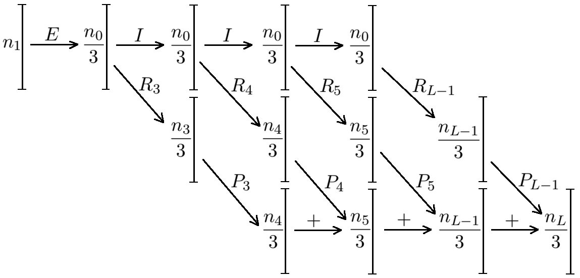
We construct by “stacking” the maps for as illustrated in Figure 2. To help us stack these maps, we drop some nodes from the original network and first construct
with some ; we can then extend trivially to . As Figure 2 suggests, we choose , , , for (skip these layers if ), , and . Note that by definition of , we indeed have for all .
We made this choice so that the network can realize the maps . As Figure 2 illustrates, the map is realized by setting the factor to map the first layer to the second, the factor to map the second layer to the last nodes of the third layer, and the factor to map further to the last nodes of the fourth layer. Moreover, the output of the second layer is transferred to the first nodes of the third layer by the identity map888Note that the identity map restricted to the image of can be realized as an almost pseudolinear map for both ReLU and threshold nonlinearities. For ReLU this is obvious by setting the bias large enough; for threshold nonlinearity note that the image of the almost pseudolinear map consists of vectors whose coordinates are either zero or take the same value . Thus, the Heaviside function multiplied by is the identity on the image of . , so we can realize the next map , and so on.
The outputs of all maps are added together as the signs “+” in Figure 2 indicate. Namely, the components of the output of , i.e. the last nodes of the fourth layer, are summed together and added to any node (say, the last node) of the fifth layer; the components of the output of , i.e. the last nodes of the fourth layer, are summed together and added to the last node of the sixth layer, and so on. For ReLU nonlinearity, the refers to addition of real numbers; for threshold nonlinearity, we replace adding by taking the maximum (i.e. the ‘OR’ operation), which is clearly realizable.
Step 5. Conclusion. Due to our construction, the sum of all components of the function computed by the network equals the sum (or maximum, for threshold nonlinearity) of all components of all functions . Since the components are always nonnegative, is zero iff all components of all functions are zero. In other words, our claim (7.7) holds. ∎
Appendix A Asymptotical expressions for Gaussian integrals
The asymptotical expansion of Mills ratio for the normal distribution is well known, see [19]. For our purposes, the first three terms of the expansion will be sufficient:
| (A.1) |
In particular, the tail probability of the standard normal random variable satisfies
| (A.2) |
The following two lemmas give asymptotical expressions for the expected value of the first two moments of the random variable where, as before, is standard normal.
Lemma A.1 (ReLU of the normal distribution).
Let . Then, as , we have
Proof.
Expressing expectation as the integral of the tail (see e.g. [22, Lemma 1.2.1]), we have
Using substitution , we see that the value of the first integral on the right hand side is . Using the Mills ratio asymptotics (A.1) for the second integral, we get
This finishes the first part of the lemma.
To prove the second part, we start similarly:
Integrating by parts, we find that the first integral on the right side equals
the second integral equals as before, and the third integral equals . Combining these and using the asymptotical expansion (A.1) for , we conclude that
This completes the proof of the second part of the lemma. ∎
Lemma A.2 (Stability).
Fix any . Let . Then, as , we have
| (A.3) | ||||
| (A.4) | ||||
| (A.5) |
We complete this paper by proving an elementary monotonicity property for Gaussian integrals, which we used in the proof of of Proposition 3.2.
Lemma A.3 (Monotonicity).
Let be a nondecreasing function satisfying for all , and let . Then is a nondecreasing function on .
Proof.
Denoting by the probability density function of , we have
The last step follows since, by assumption, for all . To complete the proof, it remains to note that for every fixed , the function is nondecreasing. ∎
References
- [1] Zeyuan Allen-Zhu, Yuanzhi Li, and Zhao Song. A convergence theory for deep learning via over-parameterization. arXiv preprint arXiv:1811.03962, 2018.
- [2] Sanjeev Arora, Simon S Du, Wei Hu, Zhiyuan Li, and Ruosong Wang. Fine-grained analysis of optimization and generalization for overparameterized two-layer neural networks. arXiv preprint arXiv:1901.08584, 2019.
- [3] Pierre Baldi and Roman Vershynin. On neuronal capacity. In Advances in Neural Information Processing Systems, pages 7729–7738, 2018.
- [4] Pierre Baldi and Roman Vershynin. The capacity of feedforward neural networks. Neural Networks, 116:288–311, 2019.
- [5] Peter L Bartlett, Nick Harvey, Christopher Liaw, and Abbas Mehrabian. Nearly-tight vc-dimension and pseudodimension bounds for piecewise linear neural networks. Journal of Machine Learning Research, 20(63):1–17, 2019.
- [6] Eric B Baum. On the capabilities of multilayer perceptrons. Journal of complexity, 4(3):193–215, 1988.
- [7] Eric B Baum and David Haussler. What size net gives valid generalization? In Advances in neural information processing systems, pages 81–90, 1989.
- [8] Thomas M Cover. Geometrical and statistical properties of systems of linear inequalities with applications in pattern recognition. IEEE transactions on electronic computers, (3):326–334, 1965.
- [9] Simon S Du, Jason D Lee, Haochuan Li, Liwei Wang, and Xiyu Zhai. Gradient descent finds global minima of deep neural networks. arXiv preprint arXiv:1811.03804, 2018.
- [10] Simon S Du, Xiyu Zhai, Barnabas Poczos, and Aarti Singh. Gradient descent provably optimizes over-parameterized neural networks. arXiv preprint arXiv:1810.02054, 2018.
- [11] Rong Ge, Runzhe Wang, and Haoyu Zhao. Mildly overparametrized neural nets can memorize training data efficiently. arXiv preprint arXiv:1909.11837, 2019.
- [12] Moritz Hardt and Tengyu Ma. Identity matters in deep learning. arXiv preprint arXiv:1611.04231, 2016.
- [13] Guang-Bin Huang. Learning capability and storage capacity of two-hidden-layer feedforward networks. IEEE Transactions on Neural Networks, 14(2):274–281, 2003.
- [14] Ziwei Ji and Matus Telgarsky. Polylogarithmic width suffices for gradient descent to achieve arbitrarily small test error with shallow relu networks. arXiv preprint arXiv:1909.12292, 2019.
- [15] Adam Kowalczyk. Estimates of storage capacity of multilayer perceptron with threshold logic hidden units. Neural networks, 10(8):1417–1433, 1997.
- [16] Yuanzhi Li and Yingyu Liang. Learning overparameterized neural networks via stochastic gradient descent on structured data. In Advances in Neural Information Processing Systems, pages 8157–8166, 2018.
- [17] GJ Mitchison and RM Durbin. Bounds on the learning capacity of some multi-layer networks. Biological Cybernetics, 60(5):345–365, 1989.
- [18] Samet Oymak and Mahdi Soltanolkotabi. Towards moderate overparameterization: global convergence guarantees for training shallow neural networks. arXiv preprint arXiv:1902.04674, 2019.
- [19] Iosif Pinelis. Monotonicity properties of the relative error of a padé approximation for mills’ ratio. J. Inequal. Pure Appl. Math, 3(2):1–8, 2002.
- [20] Zhao Song and Xin Yang. Quadratic suffices for over-parametrization via matrix chernoff bound. arXiv preprint arXiv:1906.03593, 2019.
- [21] Ruoyu Sun. Optimization for deep learning: theory and algorithms. arXiv preprint arXiv:1912.08957, 2019.
- [22] Roman Vershynin. High-dimensional probability: An introduction with applications in data science. cambridge series in statistical and probabilistic mathematics, 2018.
- [23] Masami Yamasaki. The lower bound of the capacity for a neural network with multiple hidden layers. In International Conference on Artificial Neural Networks, pages 546–549. Springer, 1993.
- [24] Chulhee Yun, Suvrit Sra, and Ali Jadbabaie. Small relu networks are powerful memorizers: a tight analysis of memorization capacity. In Advances in Neural Information Processing Systems, pages 15532–15543, 2019.
- [25] Chiyuan Zhang, Samy Bengio, Moritz Hardt, Benjamin Recht, and Oriol Vinyals. Understanding deep learning requires rethinking generalization. ICLR, 2017.
- [26] Difan Zou, Yuan Cao, Dongruo Zhou, and Quanquan Gu. Stochastic gradient descent optimizes over-parameterized deep relu networks. arXiv preprint arXiv:1811.08888, 2018.
- [27] Difan Zou and Quanquan Gu. An improved analysis of training over-parameterized deep neural networks. arXiv preprint arXiv:1906.04688, 2019.