Meridional rank of knots whose exterior is a graph manifold

Michel Boileau Aix-Marseille Université, CNRS, Centrale Marseille, I2M, UMR 7373, 13453 Marseille, France michel.boileau@univ-amu.fr , Ederson Dutra Mathematisches Seminar, Christian-Albrechts-Universität zu Kiel, Ludewig-Meyn Str. 4, 24098 Kiel, Germany dutra@math.uni-kiel.de , Yeonhee Jang Department of Mathematics, Nara Women’s University, Nara, 630-8506 Japan yeonheejang@cc.nara-wu.ac.jp and Richard Weidmann Mathematisches Seminar, Christian-Albrechts-Universität zu Kiel, Ludewig-Meyn Str. 4, 24098 Kiel, Germany weidmann@math.uni-kiel.de

Abstract.

We prove for a large class of knots that the meridional rank coincides with the bridge number. This class contains all knots whose exterior is a graph manifold. This gives a partial answer to a question of S. Cappell and J. Shaneson [11, pb 1.11].

First author partially supported by ANR projects 12-BS01-0003-01 and 12-BS01-0004-01
Second author supported by CAPES grant 13522-13-2

Let $\mathfrak{k}$ be a knot in $S^{3}$ . It is well-known that the knot group of $\mathfrak{k}$ can be generated by $b(\mathfrak{k})$ conjugates of the meridian where $b(\mathfrak{k})$ is the bridge number of $\mathfrak{k}$ . The meridional rank $w(\mathfrak{k})$ of $\mathfrak{k}$ is the smallest number of conjugates of the meridian that generate its group. Thus we always have $w(\mathfrak{k})\leq b(\mathfrak{k})$ . It was asked by S. Cappell and J. Shaneson [11, pb 1.11], as well as by K. Murasugi, whether the opposite inequality always holds, i.e. whether $b(\mathfrak{k})=w(\mathfrak{k})$ for any knot $\mathfrak{k}$ . To this day no counterexamples are known but the equality has been verified in a number of cases:

(1)

For generalized Montesinos knots this is due to Boileau and Zieschang [5].
(2)

For torus knots this is a result of Rost and Zieschang [15].
(3)

The case of knots of meridional rank $2$ (and therefore also knots with bridge number $2$ ) is due to Boileau and Zimmermann [6].
(4)

For a class of knots also refered to as generalized Montesinos knots, the equality is due to Lustig and Moriah [12].
(5)

For some iterated cable knots this is due to Cornwell and Hemminger [9].
(6)

For knots of meridional rank $3$ whose double branched cover is a graph manifold the equality can be found in [4].

The knot space of $\mathfrak{k}$ is defined as $X(\mathfrak{k}):=\overline{S^{3}-V(\mathfrak{k})}$ where $V(\mathfrak{k})$ is a regular neighborhood of $\mathfrak{k}$ in $S^{3}$ . The knot group $G(\mathfrak{k})$ of $\mathfrak{k}$ is the fundamental group of $X(\mathfrak{k})$ . We further denote by $P(\mathfrak{k})\leq G(\mathfrak{k})$ the peripheral subgroup of $\mathfrak{k}$ , i.e., $P(\mathfrak{k})=\pi_{1}\partial X(\mathfrak{k})$ .

Let $m\in P({\mathfrak{k}})$ be the meridian of $\mathfrak{k}$ , i.e. an element of $G(\mathfrak{k})$ which can be represented by a simple closed curve on $\partial X(\mathfrak{k})$ that bounds a disk in $S^{3}$ which intersects $\mathfrak{k}$ in exactly one point. In the sequel we refer to any conjugate of $m$ as a meridian of $\mathfrak{k}$ .

We call a subgroup $U\leq G(\mathfrak{k})$ meridional if $U$ is generated by finitely many meridians of $\mathfrak{k}$ . The minimal number of meridians needed to generated $U$ , denoted by $w(U)$ , is called the meridional rank of $U$ . Observe that the knot group $G(\mathfrak{k})$ is meridional and its meridional rank is equal to $w(\mathfrak{k})$ .

A meridional subgroup $U$ of meridional rank $w(U)=l$ is called tame if for any $g\in G(\mathfrak{k})$ one of the following holds:

(1)

$gP(\mathfrak{k})g^{-1}\cap U=1$ .
(2)

$gP(\mathfrak{k})g^{-1}\cap U=g\langle m\rangle g^{-1}$ and there exists meridians $m^{\prime}_{2},\ldots,m^{\prime}_{l}$ such that $U$ is generated by $\{gmg^{-1},m^{\prime}_{2},\ldots,m^{\prime}_{l}\}$ .

Definition 1.

A non-trivial knot $\mathfrak{k}$ in $S^{3}$ is called meridionally tame if any meridional subgroup $U\leq G(\mathfrak{k})$ generated by less than $b(\mathfrak{k})$ meridians is tame.

Remark 1.

If $\mathfrak{k}$ is meridionally tame, then its group cannot be generated by less than $b(\mathfrak{k})$ meridians. Hence the bridge number equals the meridional rank. Thus the question of Cappell and Shaneson has a positive answer for the class of meridionally tame knots by definition of meridional tameness.

The class of meridionally tame knots trivially contains the class of 2-bridge knots as any cyclic meridional subgroup is obviously tame. In Lemma 14 below we show that the meridional tameness of torus knots is implicit in [15] and in Proposition 1 we show that prime 3-bridge knots are meridionally tame. However it follows from [1] and the discussion at the end of Section 6 that satellite knots are in general not meridionally tame. For examples Whitehead doubles of non-trivial knots are never meridionally tame. These are prime satellite knots, whose satellite patterns have winding number zero, which is opposite to the braid patterns considered in this article. Moreover Whitehead doubles of 2-bridge knots are prime 4-bridge knots for which the question of Cappell and Shaneson has a positive answer by [4, Corollary 1.6]. There exists also connected sums of meridionally tame knots (for examples some 2-bridge knots) which are not meridionally tame. In contrast, it should be noted that we do not know any hyperbolic knots that are not meridionally tame, but it is likely that such knots exist.

In this article we consider the class of knots $\mathcal{K}$ that is the smallest class of knots that contains all meridionally tame knots and is closed under connected sums and satellite constructions with braid patterns, see Section 1 for details. The following result is our main theorem:

Theorem 1.

Let $\mathfrak{k}$ be a knot from $\mathcal{K}$ . Then $w(\mathfrak{k})=b(\mathfrak{k})$ .

As the only Seifert manifolds that can be embedded into $\mathbb{R}^{3}$ are torus knot complements, composing spaces and cable spaces (see [13]) and as cable spaces are special instances of braid patterns we immediately obtain the following consequence of Theorem 1.

Corollary 1.

Let $\mathfrak{k}$ be a knot such that its exterior is a graph manifold. Then

w(\mathfrak{k})=b(\mathfrak{k}).

In 2015 the first, third and fourth author found a proof that the meridional rank coincides with the bridge number for the easier case of knots obtained from torus knots by satellite operations with braid patterns. In the meantime the second and fourth authors introduced the notion of meridional tameness, and the second author was able to generalize the result to the broader class of knots $\mathcal{K}$ by proving Theorem 1. Some basic features of the original proof are preserved, but the proof of Theorem 1 is much more involved and subtle, in particular because of the presence of composing spaces.

1. Description of the class $\mathcal{K}$ .

In this section we introduce the appropriate formalism to study knots that lie in the class $\mathcal{K}$ introduced in the introduction. Recall that these knots are obtained from meridionally tame knots by repeatedly taking connected sums and performing satellite constructions with braid patterns.

We first discuss satellite construction with braid patterns. This generalizes the well-known cabling construction. Satellite construction with braid patterns are also discussed in [9].

Refer to caption — Figure 1. $\beta$ is the $3$ -braid $\sigma_{2}{\sigma_{1}}^{-1}\sigma_{2}^{2}$ and $\mathfrak{k}_{1}$ is the trefoil knot.

Let $V_{0}=\mathbb{D}^{2}\times S^{1}$ be a standardly embedded solid torus in ${\mathbb{R}}^{3}$ and $\beta$ an $n$ -braid with $n\geq 2$ . Assume that the closed braid $\widehat{\beta}$ is standardly embedded in the interior of $V_{0}$ , see Figure 1. For a knot $\mathfrak{k}_{1}\subset S^{3}$ and a homeomorphism $h:V_{0}\rightarrow V(\mathfrak{k}_{1})$ onto a tubular neighborhood of $\mathfrak{k}_{1}$ which sends a meridian of $V_{0}$ onto a meridian of $\mathfrak{k}_{1}$ and the longitude of $V_{0}$ (i.e. the simple closed curve on $\partial V_{0}$ that is nullhomotopic in the complement of the interior of $V_{0}$ ) to the longitude of $\mathfrak{k}$ , we define the link $\mathfrak{k}:=h(\widehat{\beta})$ , see Figure 1. Note that $\mathfrak{k}$ is a knot if and only if the associated permutation $\tau\in S_{n}$ of $\beta$ is a cycle of length $n$ . In this case the knot $\mathfrak{k}$ is called a $\beta$ -satellite of $\mathfrak{k}_{1}$ and $\mathfrak{k}$ is denote by $\beta(\mathfrak{k}_{1})$ . We also say that $\mathfrak{k}$ is obtained from $\mathfrak{k}_{1}$ by a satellite operation with braid pattern $\beta$ .

In order to define the class $\mathcal{K}$ we need some terminology.

Let $A$ be a finite tree. A subset $E\subset EA$ is called an orientation of $A$ if $EA=E\overset{.}{\cup}E^{-1}$ . For a finite rooted tree $(A,v_{0})$ we will define a natural orientation determined by the root $v_{0}$ in the following way: for each vertex $v\in VA$ there exists a unique reduced path $\gamma_{v}:=e_{v,1},\ldots,e_{v,r_{v}}$ in $A$ from $v_{0}$ to $v$ . We define

E(A,v_{0})=\{e_{v,i}\ |\ v\in VA,1\leq i\leq r_{v}\}.

Throughout this paper we assume that any rooted tree $(A,v_{0})$ is endowed with this orientation.

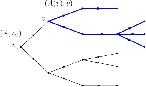
Suppose that $E$ is some orientation for $A$ . We say that a path $e_{1},\ldots,e_{k}$ in $A$ is oriented if $e_{i}\in E$ for $1\leq i\leq k$ . For any vertex $v\in VA$ we define $A(v)$ as the sub-tree of $A$ spanned by the set

VA(v)=\{\omega(\gamma)\ |\ \gamma\text{ is an oriented path in }A\text{ and }\alpha(\gamma)=v\}.

Note that for any vertex $w\in VA$ we have

E(A(w),w)=E(A,v_{0})\cap EA(w)

where we consider the canonical orientations defined above, see Figure 2.

Recall that for any vertex $v\in VA$ , the star of $v$ is defined as

St(v,A)=\{e\in EA\ |\ \alpha(e)=v\}.

The cardinality $|St(v,A)|$ of $St(v,A)$ is called the valence of $v$ , written $val(v,A)$ . If $A$ is assigned some orientation $E\subset EA$ we further define the positive star of $v$ as

St_{+}(v,A)=St(v,A)\cap E

and the positive valence of $v$ as $val_{+}(v,A)=|St_{+}(v,A)|$ .

For $i\in\{0,1\}$ we set

V_{i}:=\{v\in VA\ |\ val_{+}(v,A)=i\}

and we also define

V_{2}:=\{v\in VA\ |\ val_{+}(v,A)\geq 2\}.

We now define labelings of rooted trees. A labeled rooted tree is a tuple

\mathcal{A}=((A,v_{0}),\{\mathfrak{k}_{v}\ |\ v\in V_{0}\},\{\beta_{v}\ |\ v\in V_{1}\})

such that the following hold:

(1)

$(A,v_{0})$ is a finite rooted tree.
(2)

For any $v\in V_{0}$ , $\mathfrak{k}_{v}$ is a non-trivial knot.
(3)

For any $v\in V_{1}$ , $\beta_{v}$ is an $n_{v}$ -braid having $n_{v}\geq 2$ strands such that the closed braid $\widehat{\beta_{v}}$ is a knot.

For $w\in VA$ we define the labeled rooted tree $\mathcal{A}_{w}$ as

\mathcal{A}_{w}:=((A(w),w),\{\mathfrak{k}_{v}\ |\ v\in V_{0}\cap VA(w)\},\{\beta_{v}\ |\ v\in V_{1}\cap VA(w)\}).

We now associate to any labeled rooted tree $\mathcal{A}$ a knot $\mathfrak{k}=\mathfrak{k}_{\mathcal{A}}\subset S^{3}$ . We define $l(\mathcal{A}):=max\{d(v,v_{0})\ |\ v\in VA\}$ . We recursively define $\mathfrak{k}_{\mathcal{A}}$ in the following way:

(1)

If $l(\mathcal{A})=0$ , then we define $\mathfrak{k}_{\mathcal{A}}=\mathfrak{k}_{v_{0}}$ .
(2)

If $l(\mathcal{A})>0$ and $val(v_{0},A)=1$ , then we define $\mathfrak{k}_{\mathcal{A}}:=\beta_{v_{0}}(\mathfrak{k}_{\mathcal{A}_{v_{1}}})$ where $v_{1}\in VA$ is the unique vertex of $A$ such that $d(v_{1},v_{0})=1$ .
(3)

If $l(\mathcal{A})>0$ and $val(v_{0},A)\geq 2$ then we define $\mathfrak{k}_{\mathcal{A}}:=\overset{d}{\underset{i=1}{\sharp}}\mathfrak{k}_{\mathcal{A}_{v_{i}}}$ where $v_{1},\ldots,v_{d}\in VA$ such that $d(v_{i},v_{0})=1$ .

Note that this is a (recursive) definition indeed as in situation (2) and (3) we have $l(\mathcal{A}_{v_{i}})<l({\mathcal{A}})$ for all occurring $i$ . Note moreover that $\mathfrak{k}_{\mathcal{A}}$ lies in the class $\mathcal{K}$ if and only if $\mathfrak{k}_{v}$ is meridionally tame for any $v\in V_{0}$ . Thus we can rephrase the main theorem in the following way:

Theorem 2.

Let $\mathcal{A}$ be a labeled rooted tree and $\mathfrak{k}=\mathfrak{k}_{\mathcal{A}}$ . Suppose that $\mathfrak{k}_{v}$ is meridionally tame for all $v\in V_{0}$ . Then

b(\mathfrak{k})=w(\mathfrak{k}).

The proof relies on computing both the bridge number and the meridional rank. We conclude this section with the computation of the bridge number which is an easy consequence of the work of Schubert.

Remember that any vertex $v\in V_{1}$ is labeled $\beta_{v}$ , where $\beta_{v}$ is a braid with $n_{v}$ strands. We define the function $n:VA\rightarrow\mathbb{N}$ by

n(v)=\left\{\begin{array}[]{lcl}n_{v}&\text{if}&v\in V_{1}\\ 1&\text{if}&v\in V_{0}\cup V_{2}\\ \end{array}\right.

Recall that, for any $v\in VA$ , $\gamma_{v}=e_{v,1},\ldots,e_{v,r_{v}}$ is the unique reduced path in $A$ from $v_{0}$ to $v$ . We define the height of a vertex $v\in VA$ in $A$ as

h(v):=\prod_{i=1}^{r_{v}}n({\alpha(e_{v,i})})

for $v\neq v_{0}$ and $h(v_{0}):=1$ .

Lemma 1.

Let $\mathfrak{k}=\mathfrak{k}_{\mathcal{A}}$ be the knot defined by the labeled rooted tree $\mathcal{A}$ . Then the bridge number of $\mathfrak{k}$ is given by

b(\mathfrak{k})=\bigg{[}\sum_{v\in V_{0}}h(v)\cdot b({\mathfrak{k}}_{v})\bigg{]}-\bigg{[}\sum_{v\in V_{2}}h(v)\cdot(val_{+}(v,A)-1)\bigg{]}

The proof of the Lemma relies in the following result of Schubert [16], see also [17] for a more modern proof. Note that the result of Schubert is actually stronger than what we state.

Theorem 3 (Schubert).

Let $\mathfrak{k}_{1},\ldots,\mathfrak{k}_{d}$ be knots in $S^{3}$ and $\beta$ be an $n$ -braid such that the closed braid $\widehat{\beta}$ is a knot. Then the following hold:

(i)

$b(\mathfrak{k}_{1}\sharp\ldots\sharp\mathfrak{k}_{d})=b(\mathfrak{k}_{1})+\ldots+b(\mathfrak{k}_{d})-(d-1)$ .
(ii)

$b(\beta(\mathfrak{k}_{1}))=n\cdot b(\mathfrak{k}_{1})$ .

Proof of Lemma 1.

The proof is by induction on $l(\mathcal{A}):=max\{d(v,v_{0})\ |\ v\in VA\}$ . If $l(\mathcal{A})=0$ , then $\mathfrak{k}=\mathfrak{k}_{v_{0}}$ . Hence we have

b(\mathfrak{k})=b(\mathfrak{k}_{v_{0}})=\bigg{[}\sum_{v\in V_{0}=\{v_{0}\}}h(v)\cdot b({\mathfrak{k}}_{v})\bigg{]}-\bigg{[}\sum_{v\in V_{2}=\emptyset}h(v)\cdot(val_{+}(v,A)-1)\bigg{]}

as $h(v_{0})=1$ .

Suppose that $l(\mathcal{A})>0$ and $val_{+}(v_{0},A)=1$ . Let $v_{1}\in VA$ be the unique vertex such that $d(v_{0},v_{1})=1$ . In this case $V_{0}\cup V_{2}\subset VA(v_{1})$ . If $h_{v_{1}}$ denotes the height of a vertex in the rooted tree $(A(v_{1}),v_{1})$ , then it is easy to see that $h(v)=n({v_{0}})h_{v_{1}}(v)$ for all $v\in VA(v_{1})$ . Moreover, $val_{+}(v,A(v_{1}))=val_{+}(v,A)$ for all $v\in VA(v_{1})$ . By Theorem 3(ii) and the induction hypothesis we obtain:

$\displaystyle b(\mathfrak{k})$	$\displaystyle\overset{\text{3(ii)}}{=}$	$\displaystyle n_{v_{0}}\cdot b(\mathfrak{k}_{\mathcal{A}_{v_{1}}})$
	$\displaystyle\overset{\text{i.h.}}{=}$	$\displaystyle n_{v_{0}}\cdot\bigg{[}\sum_{v\in V_{0}\cap VA(v_{1})}h_{v_{1}}(v)\cdot b(\mathfrak{k}_{v})-$
		$\displaystyle-\sum_{v\in V_{2}\cap VA(v_{1})}h_{v_{1}}(v)\cdot(val_{+}(v,A(v_{1}))-1)\bigg{]}$
	$\displaystyle=$	$\displaystyle\sum_{v\in V_{0}\cap VA(v_{1})}n_{v_{0}}h_{v_{1}}(v)\cdot b(\mathfrak{k}_{v})-\sum_{v\in V_{2}\cap VA(v_{1})}n_{v_{0}}h_{v_{1}}(v)\cdot(val_{+}(v,A)-1)$
	$\displaystyle=$	$\displaystyle\bigg{[}\sum_{v\in V_{0}}h(v)\cdot b({\mathfrak{k}}_{v})\bigg{]}-\bigg{[}\sum_{v\in V_{2}}h(v)\cdot(val_{+}(v,A)-1)\bigg{]}$

Suppose now that $l(\mathcal{A})>0$ and $d:=val_{+}(v_{0},A)\geq 2$ . Let $v_{1},\ldots,v_{d}\in VA$ such that $d(v_{i},v_{0})=1$ . By definition, $\mathfrak{k}$ is equal to the connected sum $\overset{d}{\underset{i=1}{\sharp}}{\mathfrak{k}_{\mathcal{A}_{v_{i}}}}$ . Observe that if $h_{v_{i}}$ denotes the height of a vertex in the rooted tree $(A(v_{i}),v_{i})$ , then $h_{v_{i}}(v)=h(v)$ for any $v\in VA(v_{i})$ . By Theorem 3(i) and the induction hypothesis we obtain:

$\displaystyle b(\mathfrak{k})$	$\displaystyle\overset{\text{3(i)}}{=}$	$\displaystyle\bigg{[}\sum_{i=1}^{d}{b(\mathfrak{k}_{\mathcal{A}_{v_{i}}})}\bigg{]}-(d-1)=\bigg{[}\sum_{i=1}^{d}{b(\mathfrak{k}(\mathcal{A}_{v_{i}}))}\bigg{]}-(val_{+}(v_{0},A)-1)=$
	$\displaystyle\overset{\text{i.h.}}{=}$	$\displaystyle\bigg{[}\sum_{i=1}^{d}{\bigg{(}\sum_{v\in V_{0}\cap VA(v_{i})}h_{v_{i}}(v)b({\mathfrak{k}_{\mathcal{A}_{v_{i}}}})-\sum_{v\in V_{2}\cap VA(v_{i})}h_{v_{i}}(v)(val_{+}(v,A(v_{i}))-1)\bigg{)}}\bigg{]}-$
		$\displaystyle-(val_{+}(v_{0},A)-1)$
	$\displaystyle=$	$\displaystyle\bigg{[}\sum_{v\in V_{0}}h(v)\cdot b({\mathfrak{k}}_{v})\bigg{]}-\bigg{[}\sum_{v\in V_{2}}h(w)\cdot(val_{+}(v,A)-1)\bigg{]}$

since $V_{0}=\underset{i}{\cup}(V_{0}\cap VA(v_{i}))$ and $V_{2}=\{v_{0}\}\cup(\underset{i}{\cup}(V_{2}\cup VA(v_{i})))$ . ∎

2. Description of $G(\mathfrak{k}_{\mathcal{A}})$ .

In the previous section we have constructed a knot $\mathfrak{k}_{\mathcal{A}}$ from a labeled tree $\mathcal{A}$ . The construction implies that the knot space $X(\mathfrak{k}_{\mathcal{A}})$ contains a collection $\mathcal{T}$ of incompressible tori corresponding to the edges of $A$ such that to each vertex $v\in VA$ there corresponds a component of the complement of $\mathcal{T}$ such that the following hold:

(1)

The vertex space associated to each vertex $v\in V_{0}$ is $X(\mathfrak{k}_{v})$ .
(2)

The vertex space associated to a vertex $v\in V_{1}$ is the braid space $CS(\beta_{v})$ , see below for details.
(3)

The vertex space associated to a vertex $v\in V_{2}$ is an $r$ -fold composing space where $r=val_{+}(v,A)$ .

Thus $X(\mathfrak{k}_{\mathcal{A}})$ can be thought of as a tree of spaces. It follows from the theorem of Seifert and van Kampen that corresponding to the tree of spaces there exists a tree of groups decomposition $\mathbb{A}$ of $G(\mathfrak{k}_{\mathcal{A}})$ such that all edge groups are free Abelian of rank $2$ . It is the aim of this section to describe this tree of groups. We will first describe the vertex groups that occur in this splitting and then conclude by describing the boundary monomorphisms of the tree of groups.

(1) If $v\in V_{0}$ then the complementary component of $\mathcal{T}$ corresponding to $v$ is the knot space of $\mathfrak{k}_{v}$ . Thus we put $A_{v}:=G(\mathfrak{k}_{v})$ . Denote by $m_{v}\in P(\mathfrak{k}_{v})$ the meridian and by $l_{v}\in P(\mathfrak{k}_{v})$ the longitude of $\mathfrak{k}_{v}$ .

(2) We now describe the vertex group $A_{v}$ for $v\in V_{1}$ . Let $n:=n_{v}$ be the number of strands of the associated braid $\beta_{v}$ . By definition the associated permutation $\tau\in S_{n}$ of $\beta_{v}$ is an $n$ -cycle (equivalently the closed braid $\widehat{\beta_{v}}$ is a knot) and $\widehat{\beta_{v}}$ is standardly embedded in the interior of an unknotted solid torus $V_{0}\subset\mathbb{R}^{3}$ , see Figure 1. The braid space of $\beta_{v}$ is defined as

CS(\beta_{v}):=\overline{V_{0}-V(\beta_{v})}

where $V(\beta_{v})$ is a regular neighborhood of $\widehat{\beta_{v}}$ contained in the interior of $V_{0}$ , see Figure 3. The complementary component of $\mathcal{T}$ corresponding to $v$ is by construction homeomorphic to $CS(\beta_{v})$ .

There is an obvious fibration $CS(\beta_{v})\rightarrow S^{1}$ of $CS(\beta_{v})$ onto $S^{1}$ induced by the projection of $V_{0}=\mathbb{D}^{2}\times S^{1}$ onto the second factor. The fiber is clearly the space

X:=\mathbb{D}^{2}-Q_{n},

where $Q_{n}$ is the union of the interior of $n$ disjoint disks contained in the interior of the unit disk.

We will denote the free generators of $\pi_{1}(X)$ corresponding to the boundary paths of the removed disks by $x_{1},\ldots,x_{n}$ . This gives a natural identification of $\pi_{1}(X)$ with $F_{n}$ . We obtain the short exact sequence

1\rightarrow F_{n}=\pi_{1}(X)\rightarrow\pi_{1}(CS(\beta_{v}))\rightarrow\pi_{1}(S^{1})=\mathbb{Z}\rightarrow 1.

Let $t\in A_{v}:=\pi_{1}CS(\beta_{v})$ be the element represented by the loop in $CS(\beta_{v})$ defined by $q_{0}\times S^{1}$ , for a point $q_{0}\in\partial\mathbb{D}^{2}$ . Thus $t$ represensts a longitude of $V_{0}$ in the above sense. We can write $A_{v}$ as the semi-direct product $F_{n}\rtimes\mathbb{Z}$ where the action of $\mathbb{Z}=\langle t\rangle$ on the fundamental group of the fiber is given by

tx_{i}t^{-1}=A_{i}x_{\tau(i)}A_{i}^{-1}\ \ \ \ 1\leq i\leq n

and the words $A_{1},\ldots,A_{n}\in F_{n}$ satisfy the identity

A_{1}x_{\tau(1)}A_{1}^{-1}\cdot\ldots\cdot A_{n}x_{\tau(n)}A_{n}^{-1}=x_{1}\cdot\ldots\cdot x_{n}

in the free group $F_{n}$ .

Note that any element of $A_{v}$ can be uniquely written in the form $w\cdot t^{r}$ with $w\in F_{n}$ and $r\in\mathbb{Z}$ . Moreover

C_{v}:=\pi_{1}(\partial V_{0})=\langle x_{n+1},t\rangle

where $x_{n+1}:=x_{1}\cdot\ldots\cdot x_{n}$ . Note that in a satellite construction with braid pattern $\beta_{v}$ the curve corresponding to $x_{n+1}$ is identified with the meridian of the companion knot and the curve corresponding to $t$ is identified with the longitude of the companion knot. Finally

P_{v}:=\pi_{1}(\partial V(\beta_{v}))=\langle m_{v},l_{v}\rangle

where $m_{v}:=x_{1}$ and $l_{v}:=u\cdot t^{n}$ for some $u\in F_{n}$ . Note that for a satellite with braid patttern $\beta_{v}$ , thus in particular for the knot $\mathfrak{k}_{\mathcal{A}_{v}}$ , $m_{v}$ and $l_{v}$ represent the meridian and the longitude of the satellite knot.

Note further that $F_{n}=\langle\langle m_{v}\rangle\rangle_{A_{v}}$ (normal closure in $A_{v}$ ) as any two elements of $\{x_{1},\ldots,x_{n}\}$ are conjugate in $A_{v}$ . It follows in particular that $C_{v}\cap\langle\langle m_{v}\rangle\rangle_{A_{v}}=\langle x_{n+1}\rangle$ .

(3) We now describe the vertex group $A_{v}$ if $v\in V_{2}$ . Let $n=val_{+}(v,A)$ . By construction the complementary component of $\mathcal{T}$ corresponding to the vertex $v$ is homeomorphic to an $n$ -fold composing space $W_{n}:=X\times S^{1}$ , where $X=\mathbb{D}^{2}-Q_{n}$ is as before, see [13]. Thus

A_{v}:=\pi_{1}(W_{n})=\pi_{1}(X)\times\pi_{1}(S^{1})=\langle x_{1},\ldots,x_{n},t\ |\ [x_{i},t]=1\rangle.

Consequently any element of $A_{v}$ can be uniquely written as $w\cdot t^{z}$ with $w\in F_{n}$ and $z\in\mathbb{Z}$ . Clearly $t$ generates the center of $A_{v}$ .

If the homeomorphism is chosen appropriately then we get the following with the above notation:

(1)

$P_{v}:=\langle l_{v},m_{v}\rangle$ corresponds to the peripheral subgroup of $\mathfrak{k}_{\mathcal{A}_{v}}$ where $l_{v}:=x_{n+1}$ is the longitude and $m_{v}:=t$ is the meridian.
(2)

There exists a bijection $j:St_{+}(v,A)\rightarrow\{1,\ldots,n\}$ such that for any $e\in St_{+}(v,A)$ the subgroup $C_{e}:=\langle l_{e},m_{v}\rangle$ correponds to the peripheral subgroup of $\mathfrak{k}_{\mathcal{A}_{\omega(e)}}$ with $l_{e}:=x_{j(e)}$ the longitude and $m_{v}:=t$ the meridian.

With the notation introduced we have

A_{v}=F(\{l_{e}|e\in St_{+}(v,A)\})\times\langle m_{v}\rangle.

We further denote $F(\{l_{e}|e\in St_{+}(v,A)\}$ by $F_{v}$ .

(4) For any edge $e\in E(A,v_{0})$ the associated edge group $A_{e}$ is free Abelian generated by $\{m_{e},l_{e}\}$ .

We now describe the boundary monomorphims. For any $e\in E(A,v_{0})$ with $v:=\alpha(e)$ and $w:=\omega(e)$ the boundary monomorphism $\alpha_{e}:A_{e}\rightarrow A_{v}$ is given by:

\alpha_{e}(m_{e}^{z_{1}}\cdot l_{e}^{z_{2}})=\left\{\begin{array}[]{lcl}x_{n+1}^{z_{1}}\cdot t^{z_{2}}&\text{if}&v\in V_{1}.\\ m_{v}^{z_{1}}\cdot l_{e}^{z_{2}}&\text{if}&v\in V_{2}.\\ \end{array}\right.

while $\omega_{e}:A_{e}\rightarrow A_{w}$ is given by $\omega_{e}(m_{e}^{z_{1}}\cdot l_{e}^{z_{2}})=m_{w}^{z_{1}}\cdot l_{w}^{z_{2}}$ .

3. Vertex Groups

In this section we will study subgroups of the vertex groups $A_{v}$ of $\mathbb{A}$ for $v\in V_{1}\cup V_{2}$ . As these vertex groups are semidirect products of a finitely generated free group and $\mathbb{Z}$ we start by considering certain subgroups of the free group $F_{n}$ .

We think of $F_{n}=F(x_{1},\ldots,x_{n})$ as the group given by the presentation

\langle x_{1},\ldots,x_{n+1}\mid x_{1}\cdot\ldots\cdot x_{n+1}\rangle

and identify $F_{n}$ with $\pi_{1}(X)$ where $X$ is the $(n+1)$ -punctured sphere as before.

We will study subgroups of $F_{n}$ that are generated by finitely many conjugates of the $x_{i}$ . We call an element of $F_{n}$ peripheral if it is conjugate to $x_{i}^{z}$ for some $i\in\{1,\ldots,n+1\}$ and $z\in\mathbb{Z}$ .

Lemma 2.

Let $S=\{g_{i}x_{j_{i}}g_{i}^{-1}\mid 1\leq i\leq k\}$ with $k\geq 0$ , $g_{i}\in F_{n}$ , and $j_{i}\in\{1,\ldots,n+1\}$ for $1\leq i\leq k$ . Suppose that $U:=\langle S\rangle\neq F_{n}$ .

Then there exists $T=\{h_{l}x_{p_{l}}h_{l}^{-1}\mid 1\leq l\leq m\}$ with $m\leq k$ and $h_{l}\in F_{n}$ and $p_{l}\in\{1,\ldots,n+1\}$ for $1\leq l\leq m$ such that the following hold:

(1)

$U$ is freely generated by $T$ .
(2)

Any $h_{l}x_{p_{l}}h_{l}^{-1}$ is in U conjugate to some $g_{i}x_{j_{i}}g_{i}^{-1}$ .
(3)

Any peripheral element of $U$ is in $U$ conjugate to an element of $\langle h_{l}x_{p_{l}}h_{l}\rangle$ for some $l\in\{1,\ldots,m\}$ .

In particular $\{j_{1},\ldots,j_{k}\}=\{p_{1},\ldots,p_{m}\}$ .

Remark 2.

Note that the conclusion of Lemma 2 does not need to hold if $U=F_{n}$ . Indeed if $S=\{x_{1},\ldots,x_{n+1}\}\backslash\{x_{i}\}$ for some $i\in\{1,\ldots,n+1\}$ then $\langle S\rangle=U=F_{n}$ and $U$ has $n+1$ conjugacy classes of peripheral subgroups, it follows that conclusion (3) cannot hold.

Proof.

Let $\tilde{X}$ be the cover of $X$ corresponding to $U\leq F_{n}=\pi_{1}(X)$ . Note that the $U$ -conjugacy classes of maximal peripheral subgroups of $U$ correspond to compact boundary components of $\tilde{X}$ that finitely cover boundary components of $X$ . Note that for any $i$ the $U$ -conjugacy class of $\langle g_{i}x_{j_{i}}g_{i}^{-1}\rangle$ must correspond to a compact boundary component of $\tilde{X}$ for which the covering is of degree $1$ .

As $U$ is generated by peripheral elements it follows that the interior of $\tilde{X}$ is a punctured sphere. Note further that all but one punctures must correspond to compact boundary components of $\tilde{X}$ that cover components of $\partial X$ with degree $1$ and correspond to some $\langle g_{i}x_{j_{i}}g_{i}^{-1}\rangle$ , otherwise $U$ could not be generated by $S$ by the above remark.

We now show that $\tilde{X}$ is an infinite sheeted cover of $X$ , i.e. that the last puncture does not correspond to a compact boundary component of $\tilde{X}$ . Suppose that $\tilde{X}$ is a $q$ -sheeted cover of $X$ . As $\chi(X)=2-(n+1)=1-n$ it follows that $\chi(\tilde{X})=q(1-n)=q-qn$ . Clearly $\tilde{X}$ has at least $qn+1$ boundary components as $n$ boundary components of $X$ must have $q$ lifts each in $\tilde{X}$ . It follows that

\chi(\tilde{X})\leq 2-(qn+1)=1-qn.

Thus $q=1$ and therefore $U=F_{n}$ , a contradiction.

Thus $\tilde{X}$ is an infinite sheeted cover of $X$ whose interior is homeomorphic to a punctured sphere such that all but one punctures correspond to compact boundary components of $\tilde{X}$ and such that the conjugacy classes of peripheral subgroups of $U$ corresponding to these boundary are represented by some $\langle g_{i}x_{j_{i}}g_{i}^{-1}\rangle$ . This implies that there exists $T$ satisfying (1) and (2), indeed we take $T$ to be the tuple of elements corresponding to the compact boundary components $\tilde{X}$ . Item (3) is obvious. ∎

We now use Lemma 2 to describe subgroups of $A:=\pi_{1}CS(\beta)$ that are generated by finitely many meridians, i.e. conjugates of $x_{1}$ . Here $\beta$ is an $n$ -strand braid such that associated permutation $\tau\in S_{n}$ of $\beta$ is an $n$ -cycle. Recall that $A$ is generated by $\{x_{1},\ldots,x_{n},t\}$ , that $\langle\langle x_{1}\rangle\rangle=\langle x_{1},\ldots,x_{n}\rangle$ is free in $\{x_{1},\ldots,x_{n}\}$ and that in $A$ the element $x_{1}$ is conjugate to $x_{i}$ for $1\leq i\leq n$ . As in the previous section we denote the peripheral subgroups of $A$ by $P$ and $C$ .

Corollary 2.

Let $S=\{g_{i}x_{1}g_{i}^{-1}|1\leq i\leq k\}$ with $k\geq 0$ and $g_{i}\in A$ for $1\leq i\leq k$ . Suppose that $U:=\langle S\rangle\leq A$ .

Then either $U=\langle\langle x_{1}\rangle\rangle$ or there exists

T=\{{g^{\prime}}_{l}x_{1}{g^{\prime}}_{l}^{-1}|1\leq l\leq{m}\}

with ${m}\leq k$ and ${g^{\prime}}_{l}\in A$ for $1\leq l\leq m$ such that the following hold:

(1)

$U$ is freely generated by $T$ .
(2)
For any $g\in A$ one of the following holds:
1. (a)
  
  $gPg^{-1}\cap U=\{1\}$ .
2. (b)
  
  $gPg^{-1}\cap U=g\langle x_{1}\rangle g^{-1}$ and $gx_{1}g^{-1}$ is in $U$ conjugate to ${g^{\prime}}_{l}x_{1}{g^{\prime}}_{l}^{-1}$ for some $l\in\{1,\ldots,{m}\}$ .
(3)

For any $g\in A$ we have $gCg^{-1}\cap U=\{1\}$ .

Proof.

For any $g=u\cdot t^{r}\in A$ we have $gx_{1}g^{-1}=wx_{i}w^{-1}$ where $i=\tau^{r}(1)\in\{1,\ldots,n\}$ and $w\in F_{n}$ . Hence $S$ can be rewritten in the form

S=\{w_{1}x_{j_{1}}w_{1}^{-1},\ldots,w_{k}x_{j_{k}}w_{k}^{-1}\}

with $w_{i}\in F_{n}$ and $j_{i}\in\{1,\ldots,n\}$ for $1\leq i\leq k$ . By Lemma 2 there exists

T=\{{w^{\prime}}_{1}x_{p_{1}}{w^{\prime}}_{1}^{-1},\ldots,{w^{\prime}}_{m}x_{p_{m}}{w^{\prime}}_{m}^{-1}\}

with $m\leq k$ and ${w^{\prime}}_{l}\in F_{n}$ and $p_{l}\in\{1,\ldots,n\}$ for $1\leq l\leq m$ such that $U$ is freely generated by $T$ and that the other conclusions of Lemma 2 are satisfied. We will show that $T$ satisfies (1)-(3).

Now each $w^{\prime}_{l}x_{p_{l}}{w^{\prime}_{l}}^{-1}$ can be written as ${g^{\prime}}_{l}x_{1}{g^{\prime}}_{l}^{-1}$ for some $g^{\prime}_{l}\in A$ . Hence $T$ satisfies (1).

Note that for any $g\in A$ we have

gPg^{-1}\cap U\leq gPg^{-1}\cap F_{n}=gPg^{-1}\cap gF_{n}g^{-1}=g(P\cap F_{n})g^{-1}=g\langle x_{1}\rangle g^{-1}.

Suppose that $gPg^{-1}\cap U\neq 1$ , i.e. $gx_{1}^{z}g^{-1}\in U$ for some integer $z\neq 0$ . It follows from Lemma 2(3) and the fact that any element in a free group is contained in a unique maximal cyclic subgroup that $gx_{1}g^{-1}\in U$ and that $gx_{1}g^{-1}$ is in $U$ conjugate to ${g^{\prime}}_{l}x_{1}{g^{\prime}}_{l}^{-1}$ for some $l\in\{1,\ldots,m\}$ , thus we have shown that $T$ satisfies (2).

(3) For any $g=w\cdot t^{r}\in A$ we have

gCg^{-1}\cap U\leq gCg^{-1}\cap F_{n}=gCg^{-1}\cap gF_{n}g^{-1}=g(C\cap F_{n})g^{-1}=g\langle x_{n+1}\rangle g^{-1}.

If $gx_{n+1}^{z}g^{-1}=wx_{n+1}^{z}w^{-1}\in U$ for some integer $z\neq 0$ , then Lemma 2 implies that $wx_{n+1}^{z}w^{-1}$ is in $U$ conjugate to $w^{\prime}_{l}x_{p_{l}}^{z}{w^{\prime}}_{l}^{-1}$ for some $l$ . But this is a contradiction since in $F_{n}$ the element $x_{i}^{z}$ is not conjugate to $x_{j}^{z}$ for $i\neq j\in\{1,\ldots,n+1\}$ . ∎

We now use Lemma 2 to describe subgroups of

B=\pi_{1}W_{n}=\langle x_{1},\ldots,x_{n},t|[x_{i},t]=1\rangle

that are generated by $t$ and conjugates of the $x_{i}$ . Here $P=\langle x_{n+1},t\rangle$ and $C_{i}=\langle x_{i},t\rangle$ for $1\leq i\leq n$ .

Corollary 3.

Let $S=\{g_{i}x_{j_{i}}g_{i}^{-1}|1\leq i\leq k\}$ with $g_{i}\in B$ and $j_{i}\in\{1,\ldots,n\}$ for $1\leq i\leq k$ . Let $U:=\langle S\rangle\times\langle t\rangle\leq B$ .

Then either $U=B$ or there exists

T=\{{h}_{l}x_{p_{l}}{h}_{l}^{-1}|1\leq l\leq{m}\}

with ${m}\leq k$ , ${h}_{l}\in F_{n}$ and $p_{l}\in\{1,\ldots,n\}$ for $1\leq l\leq m$ such that the following hold:

(1)

$\{j_{1},\ldots,j_{k}\}=\{p_{1},\ldots,p_{m}\}$ .
(2)

$\langle S\rangle$ is freely generated by $T$ .
(3)
For any $g\in B$ and any $i\in\{1,\ldots,n\}$ one of the following holds:
1. (a)
  
  $gC_{i}g^{-1}\cap U=\langle t\rangle$ .
2. (b)
  
  $gC_{i}g^{-1}\cap U=gC_{i}g^{-1}=g\langle x_{i}\rangle g^{-1}\times\langle t\rangle$ and $gx_{i}g^{-1}$ is in $U$ conjugate to ${h}_{l}x_{p_{l}}{h}_{l}^{-1}$ for some $l\in\{1,\ldots,{m}\}$ . In particular $i=p_{l}$ .
(4)

For any $g\in B$ we have $gPg^{-1}\cap U=\langle t\rangle$ .

Proof.

For any $g=w\cdot t^{z}\in B$ and $1\leq i\leq n+1$ we have

gx_{i}g^{-1}=wx_{i}w^{-1}.

Hence $S$ can be rewritten in the form

S=\{w_{1}x_{j_{1}}w_{1}^{-1},\ldots,w_{k}x_{j_{k}}w_{k}^{-1}\}

with $w_{i}\in F_{n}$ for $1\leq i\leq k$ and so $\langle S\rangle\leq F_{n}=\langle x_{1},\ldots,x_{n}\rangle$ . If $\langle S\rangle=F_{n}$ then $U=B$ ; thus we may assume that $\langle S\rangle$ is a proper subgroup of $F_{n}$ . By Lemma 2 there exists

T=\{h_{1}x_{p_{1}}h_{1}^{-1},\ldots,h_{m}x_{p_{m}}h_{m}^{-1}\}

with $m\leq k$ and $h_{l}\in F_{n}$ and $p_{l}\in\{1,\ldots,n\}$ for $1\leq l\leq m$ such that $U$ is freely generated by $T$ and that (1) and (2) are satisfied. We will show that $T$ satisfies (3)-(4).

(3) Let $g\in B$ and $i\in\{1,\ldots,n\}$ . Clearly we have

\langle t\rangle\subseteq gC_{i}g^{-1}\cap U.

If $\langle t\rangle=gC_{i}g^{-1}\cap U$ there is nothing to show. Thus we may assume that $\langle t\rangle\varsubsetneq gC_{i}g^{-1}\cap U$ .

It follows that $gx_{i}^{z}g^{-1}\in U$ for some $z\neq 0$ . This clearly implies that $gx_{i}^{z}g^{-1}\in\langle S\rangle$ . It follows from Lemma 2(3) that $gx_{i}g^{-1}\in\langle S\rangle$ and that $gx_{i}g^{-1}$ is in $\langle S\rangle$ conjugate to ${h}_{l}x_{p_{l}}h_{l}^{-1}$ for some $l\in\{1,\ldots,m\}$ , thus we have shown that $T$ satisfies (3).

(4) For any $g=w\cdot t^{z}\in B$ we have

\langle t\rangle\subseteq gPg^{-1}\cap U.

If $\langle t\rangle\varsubsetneq gPg^{-1}\cap U$ then $gx_{n+1}^{z}g^{-1}=wx_{n+1}^{z}w^{-1}\in U$ for some integer $z\neq 0$ . It follows that $gx_{n+1}^{z}g^{-1}\in\langle S\rangle\leq U$ . Lemma 2 implies that $wx_{n+1}^{z}w^{-1}$ is in $\langle S\rangle$ conjugate to $h_{l}x_{p_{l}}^{z}{h}_{l}^{-1}$ for some $l$ . But this is impossible as in $F_{n}$ the element $x_{i}^{z}$ is not conjugate to $x_{j}^{z}$ for $i\neq j\in\{1,\ldots,n+1\}$ . ∎

4. Proof of the main theorem

In this section we give the proof Theorem 1 or equivalently of Theorem 2. We will show that for any knot $\mathfrak{k}$ from $\mathcal{K}$ the meridional rank $w(\mathfrak{k})$ is bounded from below by the bridge number that is given by Lemma 1.

The general idea of the proof is similar to the proof of Grushko’s theorem. Clearly there is an epimorphism from the free group of rank $w(\mathfrak{k})$ to $G(\mathfrak{k})$ that maps any basis element (of some fixed basis) to a conjugate of the meridian. This epimorphism can be a realized by a morphism of graphs of groups, see construction of $\mathcal{B}_{0}$ below. Such a morphism can be written as a product of folds and the main difficulty of a proof is to define a complexity that does not increase in the folding sequence such that comparing the complexities of the initial and the terminal graph of groups yields the claim of the theorem.

Morphisms of graphs of groups were introduced by Bass [2], we will use the related notion of $\mathbb{A}$ -graphs as presented in [18] which in turn a slight modification of the language developed in [10], in fact we assume complete familiarity with the first chapted of [18] which in particular contains a detailed description of folds as introduced by Bestvina and Feighn [3] in the language of $\mathbb{A}$ -graphs.

The proof is by contradiction, thus we assume that the knot group $G(\mathfrak{k})$ of $\mathfrak{k}$ is generated by $l:=w(\mathfrak{k})<b(\mathfrak{k})$ meridians, namely by $g_{1}mg_{1}^{-1},\ldots,g_{l}mg_{l}^{-1}$ where $g_{i}\in G(\mathfrak{k})$ for $i=1,\ldots,l$ . Since $G(\mathfrak{k})$ splits as $\pi_{1}(\mathbb{A},v_{0})$ where $\mathbb{A}$ is the tree of groups described in Section 2, we see that for $1\leq i\leq l$ the element $g_{i}$ can be written as $g_{i}=[\gamma_{i}]$ where $\gamma_{i}$ is an $\mathbb{A}$ -path from $v_{0}$ to $v_{0}$ of the form

\gamma_{i}=a_{i,0},e_{i,1},a_{i,1},e_{i,2},\ldots,a_{iq_{i}-1},e_{i,q_{i}},a_{i,q_{i}}

for some $q_{i}\geq 1$ . Observe that we do not require $\gamma_{i}$ to be reduced, otherwise we could possibly not choose $\gamma_{i}$ such that $q_{i}\geq 1$ .

We now define the $\mathbb{A}$ -graph $\mathcal{B}_{0}$ as follows:

(1)

The underlying graph $B_{0}$ is a finite tree given by:

(a) $EB_{0}:=\{f_{i,j}^{\varepsilon}\ |\ 1\leq i\leq l,1\leq j\leq q_{i},\varepsilon\in\{-1,+1\}\}$ .

(b) $VB_{0}:=\{u_{0}\}\cup\{u_{i,j}\ |\ 1\leq i\leq l,1\leq j\leq q_{i}\}$ .

(c) For $1\leq i\leq l$ the initial vertex of $f_{i,j}$ is

$\alpha(f_{i,j})=\left\{\begin{array}[]{lcl}u_{0}&\text{if}&j=1.\\ u_{i,j-1}&\text{if}&j>1.\\ \end{array}\right.$

while the terminal vertex of $f_{i,j}$ is $\omega(f_{i,j})=u_{i,j}$ for $1\leq j\leq q_{i}$ .
(2)

The graph morphism $[\cdot]:B_{0}\rightarrow A$ is given by $[f_{i,j}^{\varepsilon}]=e_{i,j}^{\varepsilon}$ .

(3)

For each $u\in VB_{0}\cup EB_{0}$ the associated group is

B_{x}=\left\{\begin{array}[]{lcl}\langle m_{v_{0}}\rangle&\text{if}&x=u_{i,q_{i}}\text{ for some }1\leq i\leq l.\\ 1&&\text{ otherwise. }\\ \end{array}\right.

(4)

For $1\leq i\leq l$ , $(f_{i,j})_{\alpha}=a_{i,j-1}$ for all $1\leq j\leq q_{i}$ while

$(f_{i,j})_{\omega}=\left\{\begin{array}[]{lcl}1&\text{if}&j<q_{i}.\\ a_{i,q_{i}}&\text{if}&j=q_{i}.\\ \end{array}\right.$

Observe that the fundamental group of the associated graph of groups $\mathbb{B}_{0}$ of $\mathcal{B}_{0}$ is freely generated by the elements

y_{i}:=[1,f_{i,1},1,\ldots,f_{i,q_{i}},m_{v_{0}},f_{i,q_{i}}^{-1},\ldots,1,f_{i,1}^{-1},1]

for $1\leq i\leq l$ . Additionally, the induced homomorphism $\phi:\pi_{1}(\mathbb{B}_{0},u_{0})\rightarrow\pi(\mathbb{A},v_{0})$ is surjective as $g_{i}mg_{i}^{-1}=\phi(y_{i})$ by our construction of $\mathcal{B}_{0}$ .

Before we continue with the proof we need some terminology. Let $\mathcal{B}$ be an arbitrary $\mathbb{A}$ -graph whose underlying graph $B$ is a finite tree. Throughout the proof we assume that $B$ has the orientation $EB_{+}:=\{f\in EB\ |\ [f]\in E(A,v_{0})\}$ .

We say that a vertex $u\in VB$ is isolated if $B_{f}=1$ for any $f\in St_{+}(u,B)$ .

We further say that a vertex $u\in VB$ is full if there exists a sub-tree $B^{\prime}$ of $B(u)$ such that the following hold:

(1)

$u\in VB^{\prime}$ .
(2)

$[\cdot]:B\rightarrow A$ maps $B^{\prime}$ isomorphically onto $A([u])$ .
(3)

$B_{x}=A_{[x]}$ for all $x\in VB^{\prime}\cup EB^{\prime}$ .

The following lemma follows immediately from the definition of fullness:

Lemma 3.

Let $\mathcal{B}$ be an $\mathbb{A}$ -graph whose underlying graph is a finite tree and $u\in VB$ . Then $u$ is full if and only if $B_{u}=A_{[u]}$ and there exists $S_{+}\subseteq St_{+}(u,B)$ such that the following hold:

(1)

$[\cdot]|_{S_{+}}:S_{+}\rightarrow St_{+}([u],A)$ is a bijection.
(2)

$B_{e}=A_{[e]}$ for all $e\in S_{+}$ .
(3)

$\omega(e)$ is full for all $e\in S_{+}$ .

Lemma 4.

Let $\mathcal{B}$ be an $\mathbb{A}$ -graph whose underlying graph is a finite tree. Assume that $\mathcal{B}_{1}$ is obtained from $\mathcal{B}$ by a fold. Then the image of any full vertex in $\mathcal{B}$ is full in $\mathcal{B}_{1}$ .

Proof.

First note that if $\mathcal{B}^{\prime}$ is a folded $\mathbb{A}$ -subgraph of $\mathcal{B}$ , then it is easy to see that $\mathcal{B}^{\prime}$ is isomorphic to its image in $\mathcal{B}_{1}$ . Assume that $u\in VB$ is a full vertex of $\mathcal{B}$ . By definition there exists a sub-tree $B^{\prime}\subseteq A(u)$ such that:

(1)

$u\in B^{\prime}$ .
(2)

$[\cdot]|_{B^{\prime}}:B^{\prime}\rightarrow A([u])$ is an isomorphism.
(3)

$B_{x}=A_{[x]}$ for all $x\in VB^{\prime}\cup EB^{\prime}$ .

The $\mathbb{A}$ -subgraph $\mathcal{B}^{\prime}$ of $\mathcal{B}$ having $B^{\prime}$ as its underlying graph is trivially folded. Thus $\mathcal{B}^{\prime}$ is isomorphic to its image in $\mathcal{B}_{1}$ and so the image of $u$ in $\mathcal{B}_{1}$ is full. ∎

Definition 2.

We call an $\mathbb{A}$ -graph $\mathcal{B}$ with associated graph of groups $\mathbb{B}$ tame if the graph $B$ underlying $\mathcal{B}$ is a finite tree and the following conditions hold:

(1)
For each $f\in EB_{+}$ with $e:=[f]$ one of the following holds:
1. (a)
  
  $B_{f}=1$ .
2. (b)
  
  $B_{f}=\langle m_{e}\rangle$ .
3. (c)
  
  $B_{f}=A_{e}=\langle m_{e},l_{e}\rangle$ and $\omega(f)\in VB$ is full.
(2)
For every vertex $u\in VB$ with $v:=[u]\in V_{0}$ one of the following holds:
1. (a)
  
  $B_{u}$ is generated by $r_{u}<b(\mathfrak{k}_{v})$ meridians of $\mathfrak{k}_{v}$ .
2. (b)
  
  $B_{u}=A_{v}=G(\mathfrak{k}_{v})$ .
(3)
For every vertex $u\in VB$ with $v:=[u]\in V_{1}$ one of the following holds:
1. (a)
  
  $B_{u}$ is freely generated by finitely many conjugates of $m_{v}$ .
2. (b)
  
  $B_{u}=A_{v}$ and $u$ is full.
(4)
For every vertex $u\in VB$ with $v:=[u]\in V_{2}$ one of the following holds:
1. (a)
  
  $B_{u}=1$ .
2. (b)
  
  There exists $S_{u}\subseteq\{f\in St_{+}(u,B)\ |\ B_{f}=A_{[f]}\}$ such that $B_{u}=F_{u}\times\langle m_{v}\rangle$ , where $F_{u}$ is freely generated by
  
  $\{g_{f}l_{[f]}g_{f}^{-1}\ |\ f\in S_{u}\}$
  
  where $g_{f}\in A_{v}$ and $f_{\alpha}l_{[f]}f_{\alpha}^{-1}$ is in $B_{u}$ conjugated to $g_{f}l_{[f]}g_{f}^{-1}$ for all $f\in S_{u}$ . Moreover, if $B_{u}=A_{v}$ then $u$ is full.
  
  Put $[S_{u}]:=\{[f]\ |\ f\in S_{u}\}\subseteq St_{+}(v,A)$ .

Next we will define the complexity of a tame $\mathbb{A}$ -graph $\mathcal{B}$ . First we need to introduce the following notion. We define the positive height of a vertex $v\in VA$ as

h_{+}(v):=h(v)n(v)

where $h(v)$ denotes the height of a vertex in $A$ defined in Section 4. Note that for any edge $e\in E(A,v_{0})$ we have $h_{+}(\alpha(e))=h(\omega(e))$ . In particular we have $h_{+}(v)=h(v)$ if $v\in V_{2}$ and $h_{+}(v)=h(v)\cdot n_{v}$ if $v\in V_{1}$ .

Definition 3.

Let $\mathcal{B}$ be a tame $\mathbb{A}$ -graph.

We define the $c_{1}$ -complexity of $\mathcal{B}$ as

c_{1}(\mathcal{B}):=\sum_{\begin{subarray}{c}u\in VB\\ u\text{ isol.}\end{subarray}}h([u])\cdot w(B_{u})-\sum_{\begin{subarray}{c}u\in VB\\ u\text{ isn't isol.}\end{subarray}}h_{+}([u])\cdot(val_{+}^{1}(u,\mathcal{B})-1)

where $val_{+}^{1}(u,\mathcal{B}):=|\{f\in St_{+}(u,B)\ |\ B_{f}\neq 1\}|$ .

We further define the $c_{2}$ -complexity of $\mathcal{B}$ as

c_{2}(\mathcal{B}):=2|EB|-|E_{2}B|-\dfrac{1}{2}|E_{1}B|

where $E_{i}B\subset EB$ denotes the set of edges whose edge group is isomorphic to $\mathbb{Z}^{i}$ for $i=1,2$ .

Lastly, the $c$ -complexity of $\mathcal{B}$ is defines as

c(\mathcal{B})=(c_{1}(\mathcal{B}),c_{2}(\mathcal{B}))\in\mathbb{N}\times\mathbb{N}.

As we want to compare complexities we endow the set $\mathbb{N}\times\mathbb{N}$ with the lexicographic order, i.e. we write $(n_{1},m_{1})<(n_{2},m_{2})$ if one of the following occurs:

(1)

$n_{1}<n_{2}$ .
(2)

$n_{1}=n_{2}$ and $m_{1}<m_{2}$ .

Observe that the $\mathbb{A}$ -graph $\mathcal{B}_{0}$ defined above is tame as $B_{x}=\{1\}$ for all $x\in VB_{0}\cup EB_{0}\setminus\{u_{i,q_{i}}|1\leq i\leq l\}$ and $B_{i,q_{i}}\leq A_{v_{0}}$ is infinite cyclic generated be the meridian $m$ of $\mathfrak{k}$ . Furthermore, $c_{1}(\mathcal{B}_{0})=l<b(\mathfrak{k})$ . Thus our assumption (which will yield a contradiction) implies that there exists a tame $\mathbb{A}$ -graph $\mathcal{B}_{0}$ with $c_{1}$ -complexity strictly smaller than the bridge number of $\mathfrak{k}=\mathfrak{k}_{\mathcal{A}}$ such that the induced homomorphism

\phi:\pi_{1}(\mathbb{B}_{0},u_{0})\rightarrow\pi_{1}(\mathbb{A},v_{0})

is an epimorphism.

Let now $\mathcal{B}$ be a tame $\mathbb{A}$ -graph such that there exists a vertex $u_{0}\in VB$ of type $v_{0}$ such that $\phi:\pi_{1}(\mathbb{B},u_{0})\rightarrow\pi_{1}(\mathbb{A},v_{0})$ is surjective and that among all such $\mathcal{B}$ the $c$ -complexity is minimal. Note that $c_{1}(\mathcal{B})\leq l<b(\mathfrak{k})$ as the $\mathbb{A}$ -graph $\mathcal{B}_{0}$ constructed above is tame and the map $\phi$ is sujective. We will prove the theorem by deriving a contradiction to this minimality assumption.

Lemma 5.

$\mathcal{B}$ is not folded.

Proof.

Assume that $\mathcal{B}$ is folded. As the map

\phi:\pi_{1}(\mathbb{B},u_{0})\rightarrow\pi_{1}(\mathbb{A},v_{0})

is surjective it follows that $\mathbb{B}$ is isomorphic to $\mathbb{A}$ , i.e. the graph morphism is bijective and that all vertex and edge groups are mapped bijectively. Observe that this implies the following:

(1)

The morphism $[\cdot]$ maps the isolated vertices of $VB$ bijectively to $V_{0}\subset VA$ . It follows in particular that for any isolated vertex $u\in VB$ we have $w(B_{u})=w(A_{[u]})=w(G(\mathfrak{k}_{[u]}))=b(\mathfrak{k}_{[u]})$ as $\mathfrak{k}_{[u]}$ is meridionally tame by assumption.
(2)

As all edge groups are non-trivial we have $val_{+}^{1}(u,\mathcal{B})=val_{+}(u,B)=val_{+}([u],A)$ for all $u\in VB$ .
(3)

If $u\in VB$ is not isolated, then either $[u]\in V_{1}$ and therefore $val_{+}^{1}(u,\mathcal{B})-1=0$ or $[u]\in V_{2}$ and therefore $h_{+}([u])=h([u])$ .

Using Lemma 1 this implies that

b(\mathfrak{k})=\bigg{[}\sum_{v\in V_{0}}h(v)\cdot b({\mathfrak{k}}_{v})\bigg{]}-\bigg{[}\sum_{v\in V_{2}}h(v)\cdot(val_{+}(v,A)-1)\bigg{]}=

=\sum_{\begin{subarray}{c}u\in VB\\ u\text{ isol.}\end{subarray}}h([u])\cdot w(B_{u})-\sum_{\begin{subarray}{c}u\in VB\\ u\text{ isn't isol.}\end{subarray}}h_{+}([u])\cdot(val_{+}^{1}(u,\mathcal{B})-1)=c_{1}(\mathcal{B})

contradicting the assumption that $c_{1}(\mathcal{B})<b(\mathfrak{k})$ .

Thus $\mathcal{B}$ is not folded. ∎

As the $\mathbb{A}$ -graph $\mathcal{B}$ is not folded, a fold can be applied to $\mathcal{B}$ . As the graph $B$ underlying $\mathcal{B}$ is a tree it follows that only folds of type IA and IIA can occur. We will only apply folds of type IIA if no fold of type IA can be applied. As any fold is a composition of finitely many auxiliary moves (that clearly preserve tameness and do not change the complexity) and an elementary move we can assume that one of the following holds:

(1)

An elementary move of type IA can be applied to $\mathcal{B}$ .
(2)

No fold of type IA can be applied to $\mathcal{B}$ but an elementary move of type IIA can be applied to $\mathcal{B}$ .

In both cases we will derive the desired contradiction to the minimality of the complexity $\mathcal{B}$ by producing a tame $\mathbb{A}$ -graph $\mathbb{B}^{\prime\prime}$ that is $\pi_{1}$ -surjective and such that $c(\mathcal{B}^{\prime\prime})<c(\mathcal{B})$ .

The following lemma will be useful when considering folds. It implies that certain type IIA folds are only possible if also a fold of type IA is possible. Because of our above choice we will therefore not need to consider such folds of type IIA.

Lemma 6.

Let $\mathcal{B}$ be a tame $\mathbb{A}$ -graph, $u\in VB$ and $v:=[u]$ . Suppose that one of the following holds:

(1)

$v\in V_{2}$ and there exists $f\in St_{+}(u,B)$ labeled $(a,e,b)$ such that $B_{f}\neq A_{e}$ and $a\alpha_{e}(l_{e})a^{-1}=al_{e}a^{-1}\in B_{u}$ .
(2)

$v\in V_{1}$ , $\langle\langle m_{v}\rangle\rangle\leq B_{u}$ and there exist distinct edges $f_{1},f_{2}\in St_{+}(u,B)$ .

Then we can apply a fold of type IA to $\mathcal{B}$ .

Proof.

(1) Note first that an element

g\in A_{v}=F_{v}\times\langle m_{v}\rangle=F(\{l_{e}\ |\ e\in St_{+}(v,A)\})\times\langle m_{v}\rangle

commutes with $l_{e}$ if and only if $g=m_{v}^{z_{1}}\cdot l_{e}^{z_{2}}=\alpha_{e}(m_{e}^{z_{1}}\cdot l_{e}^{z_{2}})$ for $z_{1},z_{2}\in\mathbb{Z}$ . This follows immediately from the fact that any maximal cyclic subgroup of $F_{v}$ and therefore also $\langle l_{e}\rangle$ is self-normalizing in $F_{v}$ .

It follows from Corollary 3(3.b) and the tameness of $\mathcal{B}$ that there exists an edge $f_{0}\in St_{+}(u,B)$ labeled $(a_{0},e,b_{0})$ such that $B_{f_{0}}=A_{e}=\langle m_{e},l_{e}\rangle$ and

al_{e}a^{-1}=ga_{0}l_{e}a_{0}^{-1}g^{-1}

for some $g\in B_{u}$ . Thus, $a_{0}^{-1}g^{-1}a$ commutes with $l_{e}$ which implies that

a_{0}^{-1}g^{-1}a=m_{v}^{z_{1}}\cdot l_{e}^{z_{2}}=\alpha_{e}(m_{e}^{z_{1}}\cdot l_{e}^{z_{2}})

for $z_{1},z_{2}\in\mathbb{Z}$ . Hence $a=ga_{0}\alpha_{e}(m_{e}^{z_{1}}l_{e}^{z_{2}})$ . Since we further have $f_{0}\neq f$ and $[f_{0}]=[f]=e$ it follows that $\mathcal{B}$ is not folded because condition (F1) is not satisfied, see p.615 from [18]. Thus we can apply a fold of type I or type III to $\mathcal{B}$ . Since the underlying graph $B$ of $\mathcal{B}$ is a tree it follows that we can apply a fold of type IA to $\mathcal{B}$ .

(2) Since $v\in V_{1}$ it follows that $St_{+}(v,A)=\{e\}$ for some $e\in EA$ and so $f_{1}$ and $f_{2}$ are of the same type. Let $(f_{i})_{\alpha}=w_{i}\cdot t^{z_{i}}$ where $w_{i}\in\langle\langle m_{v}\rangle\rangle$ and $z_{i}\in\mathbb{Z}$ for $i\in\{1,2\}$ . We can write $(f_{2})_{\alpha}\in A_{v}=F_{n_{v}}\rtimes\langle t\rangle$ as

(f_{2})_{\alpha}=w_{2}w_{1}^{-1}\cdot(f_{1})_{\alpha}\cdot t^{z_{2}-z_{1}}.

Note now that $w_{2}w_{1}^{-1}\in\langle\langle m_{v}\rangle\rangle\leq B_{u}$ and $t^{z_{2}-z_{1}}=\alpha_{e}(l_{e}^{z_{2}-z_{1}})$ since $A_{e}=\langle m_{e},l_{e}\rangle$ and $\alpha_{e}(l_{e})=t$ . Thus $\mathcal{B}$ is not folded because condition (F1) is not satisfied which implies in our context we can apply a fold of type IA to $\mathcal{B}$ . ∎

The following Lemma implies that if we apply an elementary move of type IIA in the direction of an oriented edge, we only ever add a meridian to the edge group.

Lemma 7.

Let $\mathcal{B}$ be a tame $\mathbb{A}$ -graph and $f\in EB_{+}$ labeled $(a,e,b)$ with $x:=\alpha(f)$ . Assume that no fold of type IA is applicable to $\mathcal{B}$ (i.e. condition (F1) is satisfied) and that

B_{f}\varsubsetneq\alpha_{e}^{-1}(a^{-1}B_{x}a).

Then $\alpha_{e}^{-1}(a^{-1}B_{x}a)=\langle m_{e}\rangle$ . In particular, $B_{f}=1$ .

Proof.

We first assume that $v:=\alpha(e)\in V_{1}$ . By tameness of $\mathcal{B}$ we know that $B_{x}=A_{v}$ or $B_{x}\leq\langle\langle m_{v}\rangle\rangle$ is freely generated by conjugates of $m_{v}$ .

If $B_{x}=A_{v}$ , then the tameness of $\mathcal{B}$ implies that $x$ is full. Hence there exists an edge $f_{0}\in St_{+}(x,B)$ such that $B_{f_{0}}=A_{e}$ . Since no folds of type IA are applicable to $\mathcal{B}$ , it follows from Lemma 6 that $f=f_{0}$ which implies that

\alpha_{e}^{-1}(a^{-1}B_{x}a)=\alpha_{e}^{-1}(A_{v})=A_{e}=B_{f}

contradicting the fact that $B_{f}\varsubsetneq\alpha_{e}^{-1}(a^{-1}B_{x}a)$ .

Thus $B_{x}\leq\langle\langle m_{v}\rangle\rangle$ is freely generated by conjugates of $m_{v}$ . As by hypothesis $B_{f}\varsubsetneq\alpha_{e}^{-1}(a^{-1}B_{x}a)$ it implies that $\alpha_{e}^{-1}(a^{-1}B_{x}a)$ is non-trivial. It is a consequence of Corollary 2(3) that in this case $B_{x}=\langle\langle m_{v}\rangle\rangle$ and so $\alpha_{e}^{-1}(a^{-1}B_{x}a)=\langle m_{e}\rangle$ .

Assume now that $v\in V_{2}$ . We know from Corollary 3 that one of the following holds true:

(1)

$\alpha_{e}^{-1}(a^{-1}B_{x}a)=1$
(2)

$\alpha_{e}^{-1}(a^{-1}B_{x}a)=\langle m_{e}\rangle$
(3)

$\alpha_{e}^{-1}(a^{-1}B_{x}a)=A_{e}=\langle m_{e},l_{e}\rangle$

If $\alpha_{e}^{-1}(a^{-1}B_{x}a)=A_{e}$ , then $al_{e}a^{-1}\in F_{x}$ . As by assumption $B_{f}\varsubsetneq A_{e}$ we conclude from Lemma 6(1) that a fold of type IA can be applied on $\mathcal{B}$ , a contradiction. Thus (1) or (2) occurs. As $B_{f}\varsubsetneq\alpha_{e}^{-1}(a^{-1}B_{x}a)$ it implies that $\alpha_{e}^{-1}(a^{-1}B_{x}a)$ is non-trivial and so (2) must occur. ∎

We will now deal with the two cases mentioned above. In both cases we let $\mathcal{B}^{\prime}$ be the $\mathbb{A}$ -graph obtained from $\mathcal{B}$ by the fold of type IA or IIA, respectively. After possibly applying elementary moves first we can assume that the folds are elementary.

Case 1: An elementary move of type IA can be applied to $\mathcal{B}$ : Let $\mathcal{B}^{\prime}$ be the $\mathbb{A}$ -graph obtained from $\mathcal{B}$ by this elementary move. Thus there exist distinct edges $f_{1},f_{2}\in EB$ with $\alpha(f_{i})=u\in VB$ and $l(f_{i})=(a,e,b)$ for $i\in\{1,2\}$ such that $\mathcal{B}{{}^{\prime}}$ is obtained from $\mathcal{B}$ by identifying $f_{1}$ and $f_{2}$ into a single edge $f$ . Put $x:=\omega(f_{1})$ , $y:=\omega(f_{2})$ , $v:=\alpha(e)$ and $w:=\omega(e)$ and $z:=\omega(f)$ . In particular we have ${B_{f}^{\prime}}=\langle B_{f_{1}},B_{f_{2}}\rangle$ and ${B_{z}^{\prime}}=\langle B_{x},B_{y}\rangle$ . We further denote by ${B^{\prime}}$ the underlying graph of $\mathcal{B}^{\prime}$ , see Figure 4.

Let now $\mathcal{B}^{\prime\prime}$ be the $\mathbb{A}$ -graph obtained from $\mathcal{B}^{\prime}$ by replacing the vertex group ${B_{z}^{\prime}}$ by the group ${B_{z}^{\prime\prime}}$ defined as follows:

{B_{z}^{\prime\prime}}:=\left\{\begin{array}[]{lcl}{B_{z}^{\prime}}=\langle B_{x},B_{y}\rangle&\text{if}&w\in V_{1}\cup V_{2}\text{ or }w\in V_{0}\text{ and }w({B_{x}})+w(B_{y})<b(\mathfrak{k}_{w}).\\ A_{w}=G(\mathfrak{k}_{w})&\text{if}&w\in V_{0}\text{ and }w({B_{x}})+w(B_{y})\geq b(\mathfrak{k}_{w}).\\ \end{array}\right.

From Proposition 8 of [18] it follows that $\mathcal{B}^{\prime}$ is $\pi_{1}$ -surjective which implies that $\mathcal{B}^{\prime\prime}$ is $\pi_{1}$ -surjective since $\mathcal{B}^{\prime\prime}$ is defined from $\mathcal{B}^{\prime}$ by possibly enlarging the vertex group at $z\in VB^{\prime}$ . Note that the underlying graph $B^{\prime\prime}$ of $\mathcal{B}^{\prime\prime}$ is equal to $B^{\prime}$ . Moreover, ${B_{x}^{\prime\prime}}={B_{x}}$ for all $x\in VB^{\prime\prime}\setminus\{z\}\cup EB^{\prime\prime}\setminus\{f,f^{-1}\}$ while ${B_{f}^{\prime\prime}}={B_{f}^{\prime}}=\langle B_{f_{1}},B_{f_{2}}\rangle$ .

Lemma 8.

The $\mathbb{A}$ -graph $\mathcal{B}^{\prime\prime}$ is tame.

Proof.

We first show that edge groups are as in Definition 2. From the tameness of $\mathcal{B}$ we conclude that one of the following occurs:

(1)

${B_{f}^{\prime\prime}}=1$ .
(2)

${B_{f}^{\prime\prime}}=\langle m_{e}\rangle$ .
(3)

${B_{f}^{\prime\prime}}=A_{e}$ . This occurs if and only if $B_{f_{i}}=A_{e}$ for some $i\in\{1,2\}$ . In this case $\omega(f_{i})$ is full by tameness and therefore $z$ is also full by Lemma 4.

Since the remaining edge groups do not change we conclude that edge groups are as in Definition 2.

We can easily see that $\mathcal{B}^{\prime\prime}$ is tame if $w\in V_{0}$ . Indeed, by definition ${B_{z}^{\prime\prime}}=G(\mathfrak{k}_{w})$ or ${B_{z}^{\prime\prime}}=\langle B_{x},B_{y}\rangle$ is generated by at most $w({B_{x}})+w(B_{y})<b(\mathfrak{k}_{w})$ meridians of $\mathfrak{k}_{w}$ . Hence condition (2) of Definition 2 is fulfilled.

We next show that $\mathcal{B}^{\prime\prime}$ is tame if $w\in V_{1}$ . Note first that if $B_{q}=A_{w}$ for some $q\in\{x,y\}$ , then obviously ${B_{z}^{\prime\prime}}={B_{z}^{\prime}}=A_{w}$ . Tameness of $\mathcal{B}$ implies that $q\in VB$ is full and so $z$ is full by Lemma 4.

Thus we may assume that both $B_{x}$ and $B_{y}$ are freely generated by conjugates of $m_{w}$ . It follows from Corollary 2 that ${B_{z}^{\prime\prime}}=\langle B_{x},B_{y}\rangle$ is freely generated by at most $w(B_{x})+w(B_{y})$ conjugates of $m_{w}$ . Since any subgroup of $A_{w}$ that is generated by conjugates of $m_{w}$ is contained in $\langle\langle m_{w}\rangle\rangle$ , which in turn is a proper subgroup of $A_{w}$ , we conclude that ${B_{z}^{\prime\prime}}=A_{w}$ if and only if $B_{q}=A_{w}$ for some $q\in\{x,y\}$ . Therefore $\mathcal{B}^{\prime\prime}$ is tame.

Lastly, suppose that $w\in V_{2}$ . If $B_{x}=1$ or $B_{y}=1$ , say $B_{x}=1$ , then clearly $B_{z}^{\prime\prime}=B_{y}$ and there is nothing to show. Thus we may assume that for $q\in\{x,y\}$ we have $B_{q}=F_{q}\times\langle m_{w}\rangle$ with

F_{q}=F(\{g_{f^{\prime}}l_{[f^{\prime}]}g_{f^{\prime}}^{-1}\ |\ f^{\prime}\in S_{q}\})

where $S_{q}\subseteq\{f^{\prime}\in St_{+}(q,B)\ |\ B_{f^{\prime}}=A_{[f^{\prime}]}\}$ and $g_{f^{\prime}}\in A_{w}$ for all $f^{\prime}\in S_{q}$ . Thus $B_{z}^{\prime\prime}=F_{z}^{\prime\prime}\times\langle m_{w}\rangle$ where

F_{z}^{\prime\prime}:=\langle\{g_{f^{\prime}}l_{[f^{\prime}]}g_{f^{\prime}}^{-1}\ |\ f^{\prime}\in S_{x}\cup S_{y}\}\rangle\leq F_{w}.

From Corollary 3 we conclude that there exists a subset $S_{z}^{\prime\prime}\subseteq S_{x}\overset{.}{\cup}S_{y}$ such that

F_{z}^{\prime\prime}=F(\{h_{f^{\prime}}l_{[f^{\prime}]}h_{f^{\prime}}^{-1}\ |\ f^{\prime}\in S_{z}^{\prime\prime}\})

and $h_{f^{\prime}}l_{[f^{\prime}]}h_{f^{\prime}}^{-1}$ is in $B_{z}$ conjugated to $g_{f^{\prime}}l_{[f^{\prime}]}g_{f^{\prime}}^{-1}$ for all $f^{\prime}\in S_{z}^{\prime\prime}$ . From tameness we know that $(f^{\prime})_{\alpha}l_{[f^{\prime}]}(f^{\prime})_{\alpha}^{-1}$ is conjugated to $g_{f^{\prime}}l_{[f^{\prime}]}g_{f^{\prime}}^{-1}$ and so it is also conjugated to $h_{f^{\prime}}l_{[f^{\prime}]}h_{f^{\prime}}^{-1}$ .

We next show that $S_{z}^{\prime\prime}$ is preserved by the fold, i.e. that $S_{z}^{\prime\prime}$ is mapped injectively into $St_{+}(z,B^{\prime\prime})$ . This is trivial if $f_{1},f_{2}\in EB_{+}$ since

St_{+}(z,B^{\prime\prime})=St_{+}(x,B)\overset{.}{\cup}St_{+}(y,B).

If $f_{1},f_{2}\in EB\setminus EB_{+}$ , then it is clear that

St_{+}(z,B^{\prime\prime})=(St_{+}(x,B)\setminus\{{f_{1}}^{-1}\})\cup(St_{+}(y,B)\setminus\{{f_{2}}^{-1}\})\cup\{f^{-1}\}.

As $F_{z}^{\prime\prime}$ is free on the set $\{h_{f^{\prime}}l_{[f^{\prime}]}h_{f^{\prime}}^{-1}\ |\ f^{\prime}\in S_{z}^{\prime\prime}\}$ and $l(f_{i}^{-1})=(b^{-1},e^{-1},a^{-1})$ for $i=1,2$ , we conclude that $S_{z}^{\prime\prime}$ contains at most one element of $\{f_{1}^{-1},f_{2}^{-1}\}$ which implies that $S_{z}^{\prime\prime}$ is mapped injectively into $St_{+}(z,B^{\prime\prime})$ .

Finally we need to show that $z$ is full if $B_{z}=A_{w}$ . Observe that if $F_{z}^{\prime\prime}=F_{w}$ then $[S_{z}^{\prime\prime}]=St_{+}(w,A)$ as $F_{w}$ is freely generated by $\{l_{e}\hskip 1.42262pt|\hskip 1.42262pte\in St_{+}(w,A)\}$ . Thus there exists

S_{+}^{\prime\prime}\subseteq S_{z}^{\prime\prime}\subseteq\{f^{\prime}\in St_{+}(z,B^{\prime\prime})\ |\ B_{f^{\prime}}=A_{[f^{\prime}]}\}

such that $[\cdot]:B^{\prime\prime}\rightarrow A$ maps $S_{+}^{\prime\prime}$ bijectively onto $St_{+}(w,A)$ . From Lemma 4 we conclude that for all $f^{\prime}\in S_{+}^{\prime\prime}$ the vertex $\omega(f^{\prime})$ is full in $\mathcal{B}^{\prime\prime}$ as it is full in $\mathcal{B}$ and hence $z$ is full in $\mathcal{B}^{\prime\prime}$ by Lemma 3. ∎

Lemma 9.

$c(\mathcal{B}^{\prime\prime})<c(\mathcal{B})$ .

Proof.

Case i(a): Assume that $f_{1},f_{2}\in EB_{+}$ and $B_{f_{1}}=1$ or $B_{f_{2}}=1$ .

If $x$ and $y$ are isolated in $\mathcal{B}$ , then obviously $z$ is isolated in $\mathcal{B}^{\prime\prime}$ and we clearly have $w(B_{z}^{\prime\prime})\leq w(B_{z})+w(B_{y})$ . Thus

c_{1}(\mathcal{B}^{\prime\prime})=c_{1}(\mathcal{B})-h(w)w(B_{x})-h(w)w(B_{y})+h(w)w(B_{z})\leq c_{1}(\mathcal{B}).

If one of the vertices $x$ or $y$ , say $x$ , is not isolated in $\mathcal{B}$ , then $z$ is not isolated in $\mathcal{B}^{\prime\prime}$ . In this case we have $val_{+}^{1}(z,\mathcal{B}^{\prime\prime})=val_{+}^{1}(x,\mathcal{B})+val_{+}^{1}(y,\mathcal{B})$ and consequently

c_{1}(\mathcal{B}^{\prime\prime})=\left\{\begin{array}[]{lcl}c_{1}(\mathcal{B})-h(w)w(B_{y})&\text{if}&y\text{ is isolated in }\mathcal{B}.\\ c_{1}(\mathcal{B})-h_{+}(w)&\text{if}&y\text{ isn't isolated in }\mathcal{B}.\end{array}\right.

Since $w(B_{y})\geq 0$ and $h_{+}(w)\geq h(w)\geq 1$ we get $c_{1}(\mathcal{B}^{\prime\prime})\leq c_{1}(\mathcal{B})$ .

As at least one of the edges involved on the fold has trivial group we obtain

c_{2}(\mathcal{B}^{\prime\prime})=c_{2}(\mathcal{B})-4.

Therefore $c(\mathcal{B}^{\prime\prime})<c(\mathcal{B})$ .

Case i(b): Assume that $f_{1},f_{2}\in EB_{+}$ and $B_{f_{1}}\neq 1\neq B_{f_{2}}$ . Thus

val_{+}^{1}(u,\mathcal{B}^{\prime\prime})=val_{+}^{1}(u,\mathcal{B})-1.

If both $x$ and $y$ are isolated in $\mathcal{B}$ , then clearly $z$ is isolated in $\mathcal{B}^{\prime\prime}$ . Moreover, $w(B_{z}^{\prime\prime})\leq w(B_{x})+w(B_{y})-1$ . Indeed, for $w\in V_{0}$ the inequality follows from the fact that $\mathfrak{k}_{w}$ is meridionally tame and $B_{f_{i}}\neq 1$ for $i\in\{1,2\}$ . For $w\in V_{1}\cup V_{2}$ we know from the tameness of $\mathcal{B}$ that $B_{q}$ is generated by conjugates of $m_{w}$ since $q$ is isolated. Thus $B_{f_{i}}=\langle m_{e}\rangle$ since otherwise the vertex $\omega(f_{i})$ is full. Hence for $w\in V_{1}$ the inequality follows from Corollary 2(2.b) and for $w\in V_{2}$ this is trivial since $B_{x}=B_{y}=\langle m_{w}\rangle$ and hence $B_{z}^{\prime\prime}=\langle m_{w}\rangle$ . As $h_{+}(v)=h(w)$ we obtain

$\displaystyle c_{1}(\mathcal{B}^{\prime\prime})$	$\displaystyle=$	$\displaystyle c_{1}(\mathcal{B})+h(w)(w(B_{z})-w(B_{x})-w(B_{y}))+$
		$\displaystyle+h_{+}(v)(val_{+}^{1}(u,\mathcal{B})-val_{+}^{1}(u,\mathcal{B}^{\prime\prime}))$
	$\displaystyle\leq$	$\displaystyle c_{1}(\mathcal{B})-h(w)+h_{+}(v)$
	$\displaystyle=$	$\displaystyle c_{1}(\mathcal{B}).$

Now suppose that $x$ is not isolated in $\mathcal{B}$ , the case that $y$ is not isolated in $\mathcal{B}$ is analogous. Hence $z$ is not isolated in $\mathcal{B}^{\prime\prime}$ . Note that

val_{+}^{1}(z,\mathcal{B}^{\prime\prime})=val_{+}^{1}(x,\mathcal{B})+val_{+}^{1}(y,\mathcal{B})

and $h_{+}(v)=h(w)\leq h_{+}(w)$ . Since $B_{f_{2}}$ is non-trivial it follows that $w(B_{y})\geq 1$ . Thus if $y$ is isolated in $\mathcal{B}$ we obtain

c_{1}(\mathcal{B}^{\prime\prime})=c_{1}(\mathcal{B})-h(w)w(B_{y})+h_{+}(v)=c_{1}(\mathcal{B})+h(w)(1-w(B_{y}))\leq c_{1}(\mathcal{B}).

If $y$ is not isolated in $\mathcal{B}$ then

c_{1}(\mathcal{B}^{\prime\prime})=c_{1}(\mathcal{B})-h_{+}(w)+h_{+}(v)\leq c_{1}(\mathcal{B}).

Since $c_{2}(\mathcal{B}^{\prime\prime})\leq c_{2}(\mathcal{B})-2$ we conclude that the $c$ -complexity decreases.

Case ii: Suppose that $f_{1},f_{2}\in EB\setminus EB_{+}$ .

Initially observe that if $x$ and $y$ are isolated in $\mathcal{B}$ then $z$ is isolated in $\mathcal{B}^{\prime\prime}$ and we clearly have $w(B_{z}^{\prime\prime})\leq w(B_{x})+w(B_{y})$ . Hence

c_{1}(\mathcal{B}^{\prime\prime})=c_{1}(\mathcal{B})-h(w)(w(B_{x})+w(B_{y})-w(B_{z}))\leq c_{1}(\mathcal{B}).

If $x$ or $y$ , say $x$ , is not isolated in $\mathcal{B}$ then $z$ is not isolated in $\mathcal{B}^{\prime\prime}$ . Furthermore, we have

val_{+}^{1}(z,\mathcal{B}^{\prime\prime})=\left\{\begin{array}[]{lcl}val_{+}^{1}(x,\mathcal{B})+val_{+}^{1}(y,\mathcal{B})&\text{if}&B_{f_{1}}=1\text{ or }B_{f_{2}}=1.\\ val_{+}^{1}(x,\mathcal{B})+val_{+}^{1}(y,\mathcal{B})-1&\text{if}&B_{f_{1}}\neq 1\text{ and }B_{f_{2}}\neq 1.\\ \end{array}\right.

If $y$ is isolated in $\mathcal{B}$ , then a simple calculation shows that

c_{1}(\mathcal{B}^{\prime\prime})=c_{1}(\mathcal{B})-h(w)w(B_{y}).

If $y$ is not isolated in $\mathcal{B}$ then we see that

c_{1}(\mathcal{B}^{\prime\prime})=\left\{\begin{array}[]{lcl}c_{1}(\mathcal{B})-h_{+}(w)&\text{if}&B_{f_{1}}=1\text{ or }B_{f_{2}}=1.\\ c_{1}(\mathcal{B})&\text{ if}&B_{f_{1}}\neq 1\text{ and }B_{f_{2}}\neq 1.\end{array}\right.

Since $h_{+}(w)\geq h(w)\geq 1$ and $w(B_{y})\geq 0$ it follows that $c_{1}(\mathcal{B}^{\prime\prime})\leq c_{1}(\mathcal{B})$ . In any case the $c_{2}$ -complexity decreases by at least two so that the $c$ -complexity decreases. ∎

Case 2: No fold of type IA can be applied to $\mathcal{B}$ but an elementary move of type IIA can be applied to $\mathcal{B}$ : Let $\mathcal{B}^{\prime}$ be the $\mathbb{A}$ -graph obtained from $\mathcal{B}$ by this elementary move. Hence there is an edge $f\in EB$ with label $(a,e,b)$ , initial vertex $x=\alpha(f)$ labeled $(B_{x},v)$ and terminal vertex $y=\omega(f)$ labeled $(B_{y},w)$ such that

B_{f}\neq\alpha_{e}^{-1}(a^{-1}B_{x}a).

We will distinguish two cases depending on whether $f\in EB_{+}$ or $f\in EB\setminus EB_{+}$ .

Case i: Assume that $f\in EB_{+}$ .

It follows from Lemma 7 that $B_{f}=1$ and $\alpha_{e}^{-1}(a^{-1}B_{x}a)=\langle m_{e}\rangle$ . Denote by $\mathcal{B}^{\prime}$ the $\mathbb{A}$ -graph obtained from $\mathcal{B}$ by this fold, i.e. we replace $B_{f}=1$ by $B_{f}^{\prime}:=\langle m_{e}\rangle$ and $B_{y}$ by ${B_{y}^{\prime}}:=\langle B_{y},b^{-1}\omega_{e}(m_{e})b\rangle=\langle B_{y},b^{-1}m_{w}b\rangle$ . From Proposition 8 of [18] it follows that $\mathcal{B}^{\prime}$ is $\pi_{1}$ -surjective.

Let now $\mathcal{B}^{\prime\prime}$ be the $\mathbb{A}$ -graph obtained from $\mathcal{B}^{\prime}$ by replacing the vertex group $B_{y}^{\prime}$ by the group $B_{y}^{\prime\prime}$ defined as follows:

{B_{y}^{\prime\prime}}:=\left\{\begin{array}[]{lcl}{B_{y}^{\prime}}&\text{if}&w\in V_{1}\cup V_{2}\text{ or }w\in V_{0}\text{ and }w({B}_{y})+1<b(\mathfrak{k}_{w}).\\ G(\mathfrak{k}_{w})&\text{if}&w\in V_{0}\text{ and }w({B}_{y})+1\geq b(\mathfrak{k}_{w}).\\ \end{array}\right.

Observe that the underlying graphs of $\mathcal{B}^{\prime}$ and $\mathcal{B}^{\prime\prime}$ are both equal to the underlying graph $B$ of $\mathcal{B}$ . Moreover, $B^{\prime\prime}_{u}=B_{u}$ for all $u\in VB\setminus\{y\}\cup EB\setminus\{f,f^{-1}\}$ while $B^{\prime\prime}_{f}=B^{\prime}_{f}=\langle m_{e}\rangle$ . By the same reasons as before we see that $\mathcal{B}^{\prime\prime}$ is $\pi_{1}$ -surjective.

Lemma 10.

The $\mathbb{A}$ -graph $\mathcal{B}^{\prime\prime}$ is tame.

Proof.

Edge groups are as in Definition 2 as ${B_{f}^{\prime\prime}}=\langle m_{e}\rangle$ and the remaining edge groups do not change.

It is trivial to see that the vertex group $B_{x}$ is as in Definition 2 since $B_{x}^{\prime\prime}=B_{x}$ and $B^{\prime\prime}_{f}=\langle m_{e}\rangle$ .

It remains to check that the tameness condition is satisfied for $B^{\prime\prime}_{y}$ . If $[y]=w\in V_{0}$ then this is immediate as ${B_{y}^{\prime\prime}}=G(\mathfrak{k}_{w})$ or ${B_{y}^{\prime\prime}}$ is generated by at most $w(B_{y})+1<b(\mathfrak{k}_{w})$ meridians.

We now show that $\mathcal{B}^{\prime\prime}$ is tame if $w\in V_{1}$ . Note first that $B_{y}=A_{w}$ clearly implies ${B_{y}^{\prime\prime}}=\langle B_{y},b^{-1}m_{w}b\rangle=A_{w}$ . From tameness it follows that $y$ is full and consequently $y$ is full in $\mathcal{B}^{\prime\prime}$ by Lemma 4. Assume now that $B_{y}$ is freely generated by $w(B_{y})$ conjugates of $m_{w}$ . It follows from Corollary 2 that ${B_{y}^{\prime\prime}}=\langle B_{y},b^{-1}m_{w}b\rangle$ is freely generated by at most $w(B_{y})+1$ conjugates of $m_{w}$ and so is a proper subgroup of $A_{w}$ . Thus we have showed that $\mathcal{B}^{\prime\prime}$ is tame if $w\in V_{1}$ .

Finally we show that $\mathcal{B}^{\prime\prime}$ is tame if $w\in V_{2}$ . This case is trivial since $B_{f^{\prime}}^{\prime\prime}=B_{f^{\prime}}$ for all $f^{\prime}\in St_{+}(y,B)$ and

{B_{y}^{\prime\prime}}:=\left\{\begin{array}[]{lcl}\langle m_{w}\rangle&\text{if}&B_{y}=1.\\ B_{y}&\text{if}&B_{y}\neq 1.\\ \end{array}\right.

∎

Lemma 11.

$c(\mathcal{B}^{\prime\prime})<c(\mathcal{B})$ .

Proof.

In order to compute the complexity recall that $B_{f}=1$ is replaced by ${B_{f}^{\prime\prime}}=\langle m_{e}\rangle$ which implies that $val_{+}^{1}(x,\mathcal{B}^{\prime\prime})=val_{+}^{1}(x,\mathcal{B})+1$ .

If $y$ is not isolated in $\mathcal{B}$ , then $y$ is not isolated in $\mathcal{B}^{\prime\prime}$ . A straightforward calculation shows that

c_{1}(\mathcal{B}^{\prime\prime})=\left\{\begin{array}[]{lcl}c_{1}(\mathcal{B})-h(v)w(B_{x})&\text{if}&x\text{ is isolated in }\mathcal{B}.\\ c_{1}(\mathcal{B})-h_{+}(v)&\text{if}&x\text{ isn't isolated in }\mathcal{B}.\end{array}\right.

As $w(B_{x})\geq 1$ and $h_{+}(v)\geq h(v)\geq 1$ we obtain $c_{1}(\mathcal{B}^{\prime\prime})<c_{1}(\mathcal{B})$ .

Assume now that $y$ is isolated in $\mathcal{B}$ which implies that $y$ is isolated in $\mathcal{B}^{\prime\prime}$ . For the case in which $v\in V_{1}$ it was showed in the proof of Lemma 7 that $B_{x}=\langle\langle m_{v}\rangle\rangle$ . Since no fold of type IA is applicable to $\mathcal{B}$ , Lemma 6 implies that $St_{+}(x,B)=\{f\}$ . Hence the vertex $x$ is isolated in $\mathcal{B}$ and its contribution to the $c_{1}$ -complexity is $h([x])w(B_{x})=h(v)n_{v}=h_{+}(v)=h(w)$ . It is now easy to see that

$\displaystyle c_{1}(\mathcal{B}^{\prime\prime})$	$\displaystyle=$	$\displaystyle c_{1}(\mathcal{B})-h(v)n_{v}-h(w)w(B_{y})+h(w)w({B_{y}^{\prime\prime}})$
	$\displaystyle=$	$\displaystyle c_{1}(\mathcal{B})-h(w)(1+w(B_{y})+w(B^{\prime\prime}_{y}))$
	$\displaystyle\leq$	$\displaystyle c_{1}(\mathcal{B})$

as $w({B_{y}^{\prime\prime}})=w(\langle B_{y},b^{-1}m_{w}b\rangle)\leq w(B_{y})+1$ .

Let us now consider that case in which $v\in V_{2}$ . If $x$ is isolated in $\mathcal{B}$ , then its contribution to the $c_{1}$ -complexity of $\mathcal{B}$ is $h(v)$ since in this case the tameness of $\mathcal{B}$ tells us that $B_{x}=\langle m_{v}\rangle$ . A simple calculation shows that

c_{1}(\mathcal{B}^{\prime\prime})=c_{1}(\mathcal{B})-h(v)-h(w)w(B_{y})+h(w)w(\langle B_{y},b^{-1}m_{w}b\rangle).

Since $h(w)=h(v)$ we conclude that $c_{1}(\mathcal{B}^{\prime\prime})\leq c_{1}(\mathcal{B})$ .

If $x$ is not isolated in $\mathcal{B}$ , then $c_{1}(\mathcal{B}^{\prime\prime})\leq c_{1}(\mathcal{B})$ as $h_{+}(v)=h(w)$ .

Finally, as $c_{2}(\mathcal{B}^{\prime\prime})=c_{2}(\mathcal{B})-1$ it implies that $c(\mathcal{B}^{\prime\prime})<c(\mathcal{B})$ . ∎

Case ii: Assume now that $f\in EB\setminus EB_{+}$ . Note that in this case $w\notin V_{0}$ . The fact that the fold is possible, combined with Corollaries 2 and 3, imply that one of the following occurs:

(1)

$\alpha_{e}^{-1}(a^{-1}B_{x}a)=\langle m_{e}\rangle$ .
(2)

$\alpha_{e}^{-1}(a^{-1}B_{x}a)=A_{e}=\langle m_{e},l_{e}\rangle$ . This occurs iff $B_{x}=A_{v}$ .

Denote by $\mathcal{B}^{\prime}$ the $\mathbb{A}$ -graph obtained from $\mathcal{B}$ by this fold, i.e. we replace $B_{f}$ by ${B_{f}^{\prime}}$ defined as follows:

{B_{f}^{\prime}}:=\left\{\begin{array}[]{lcl}\langle m_{e}\rangle&\text{if}&\alpha_{e}^{-1}(a^{-1}B_{x}a)=\langle m_{e}\rangle.\\ A_{e}&\text{if}&\alpha_{e}^{-1}(a^{-1}B_{x}a)=A_{e}.\\ \end{array}\right.

and the vertex group $B_{y}$ by ${B_{y}^{\prime}}$ defined as

{B_{y}^{\prime}}:=\left\{\begin{array}[]{lcl}\langle B_{y},b^{-1}\omega_{e}(m_{e})b\rangle&\text{if}&\alpha_{e}^{-1}(a^{-1}B_{x}a)=\langle m_{e}\rangle.\\ \langle B_{y},b^{-1}\omega_{e}(m_{e})b,b^{-1}\omega_{e}(l_{e})b\rangle&\text{if}&\alpha_{e}^{-1}(a^{-1}B_{x}a)=A_{e}.\\ \end{array}\right.

Once again, it follows from Proposition 8 of [18] that $\mathcal{B}^{\prime}$ is $\pi_{1}$ -surjective.

Let $\mathcal{B}^{\prime\prime}$ be the $\mathbb{A}$ -graph obtained from $\mathcal{B}^{\prime}$ by replacing the vertex group ${B_{y}^{\prime}}$ by ${B_{y}^{\prime\prime}}$ defined as follows:

{B_{y}^{\prime\prime}}:=\left\{\begin{array}[]{lcl}{B_{y}^{\prime}}&\text{if}&w\in V_{2}.\\ \langle\langle m_{w}\rangle\rangle&\text{if}&\alpha_{e}^{-1}(a^{-1}B_{x}a)=\langle m_{e}\rangle\text{ and }w\in V_{1}.\\ A_{w}&\text{if}&\alpha_{e}^{-1}(a^{-1}B_{x}a)=A_{e}\text{ and }w\in V_{1}.\\ \end{array}\right.

We remark that $\mathcal{B}^{\prime\prime}$ is $\pi_{1}$ -surjective as it is defined from the $\pi_{1}$ -surjective $\mathbb{A}$ -graph $\mathcal{B}^{\prime}$ by possibly enlarging the vertex group at $y$ .

Lemma 12.

The $\mathbb{A}$ -graph $\mathcal{B}^{\prime\prime}$ is tame.

Proof.

Note that ${B_{f}^{\prime\prime}}={B_{f}^{\prime}}=\langle m_{e}\rangle$ or ${B_{f}^{\prime\prime}}={B_{f}^{\prime}}=A_{e}=\langle m_{e},l_{e}\rangle$ . The latter case occurs only when $B_{x}=A_{v}$ . By tameness it follows that $x$ is full in $\mathcal{B}$ and hence $x$ is full in $\mathcal{B}^{\prime\prime}$ by Lemma 4.

The $\mathbb{A}$ -graph $\mathcal{B}^{\prime\prime}$ is obviously tame if $w\in V_{1}$ since by definition ${B_{y}^{\prime\prime}}=\langle\langle m_{w}\rangle\rangle$ or ${B_{y}^{\prime\prime}}=A_{w}$ . The latter case occurs only when $B_{x}=A_{v}$ and so ${B_{f}^{\prime\prime}}=A_{e}$ . As $f^{-1}\in St_{+}(y,B)$ and $St_{+}(w,A)=\{e^{-1}\}$ we conclude from Lemma 3 that $y$ is full in $\mathcal{B}^{\prime\prime}$ .

Finally we show that $\mathcal{B}^{\prime\prime}$ is tame if $w\in V_{2}$ . It is trivial to see that $\mathcal{B}^{\prime\prime}$ is tame if $\alpha_{e}^{-1}(a^{-1}B_{x}a)=\langle m_{e}\rangle$ since in this situation we have

{B_{y}^{\prime\prime}}:=\left\{\begin{array}[]{lcl}\langle m_{w}\rangle&\text{if}&B_{y}=1.\\ B_{y}&\text{if}&B_{y}\neq 1.\\ \end{array}\right.

It is also trivial to see that $\mathcal{B}^{\prime\prime}$ is tame if $\alpha_{e}^{-1}(a^{-1}B_{x}a)=A_{e}$ and $B_{y}\leq\langle m_{w}\rangle$ since in this case ${B_{y}^{\prime\prime}}=\langle b^{-1}l_{e^{-1}}b\rangle\times\langle m_{w}\rangle\varsubsetneq A_{w}$ . So assume that $\alpha_{e}^{-1}(a^{-1}B_{x}a)=A_{e}$ and $B_{y}=F_{y}\times\langle m_{w}\rangle$ where $F_{y}$ is freely generated by

\{g_{f^{\prime}}l_{[f^{\prime}]}g_{f^{\prime}}^{-1}\ |\ f^{\prime}\in S_{y}\}.

Thus

{B_{y}^{\prime\prime}}={F_{y}^{\prime\prime}}\times\langle m_{w}\rangle

where

{F_{y}^{\prime\prime}}:=\langle\{b^{-1}l_{e^{-1}}b\}\cup\{g_{f^{\prime}}l_{[f^{\prime}]}g_{f^{\prime}}^{-1}\ |\ f^{\prime}\in S_{y}\}\rangle.

Corollary 3 implies that there exists a subset ${S_{y}^{\prime\prime}}\subseteq S_{y}\cup\{f^{-1}\}$ such that ${F_{y}^{\prime\prime}}$ is freely generated by $\{h_{f^{\prime}}l_{[f^{\prime}]}h_{f^{\prime}}^{-1}\ |\ f^{\prime}\in{S_{y}^{\prime\prime}}\}$ and $h_{f^{\prime}}l_{[f^{\prime}]}h_{f^{\prime}}^{-1}$ is in ${B_{y}^{\prime\prime}}$ is conjugated to $g_{f^{\prime}}l_{[f^{\prime}]}g_{f^{\prime}}^{-1}$ or to $b^{-1}l_{e^{-1}}b$ . If ${B_{y}^{\prime\prime}}=A_{w}$ then ${F_{y}^{\prime\prime}}=F_{w}$ which implies that $[{S_{y}^{\prime\prime}}]=St_{+}(w,A)$ . Combining Lemmas 3 and 4 and the tameness of $\mathcal{B}$ we conclude that $y$ is full in $\mathcal{B}^{\prime\prime}$ . Therefore $\mathcal{B}^{\prime\prime}$ is tame if $w\in V_{2}$ . ∎

Lemma 13.

$c(\mathcal{B}^{\prime\prime})<c(\mathcal{B})$ .

Proof.

Note that if $y$ is isolated in $\mathcal{B}$ , then we obtain

c_{1}(\mathcal{B}^{\prime\prime})=c_{1}(\mathcal{B})-h(w)w(B_{y})\leq c_{1}(\mathcal{B})

since $y$ is not isolated in $\mathcal{B}^{\prime\prime}$ and $val_{+}^{1}(y,\mathcal{B}^{\prime\prime})=1$ .

If $y$ is not isolated in $\mathcal{B}$ , then $val_{+}^{1}(y,\mathcal{B}^{\prime\prime})\geq val_{+}^{1}(y,\mathcal{B})$ . Thus

c_{1}(\mathcal{B}^{\prime\prime})=c_{1}(\mathcal{B})+h_{+}(w)(val_{+}^{1}(y,\mathcal{B})-1)-h_{+}(w)(val_{+}^{1}(y,\mathcal{B}^{\prime\prime})-1)\leq c_{1}(\mathcal{B}).

In both cases a simple calculation shows that $c_{2}(\mathcal{B}^{\prime\prime})\leq c_{2}(\mathcal{B})-1$ which implies that the $c$ -complexity decreases. ∎

5. Meridional tameness of torus knots

In this section we show that torus knots are meridionally tame. This fact is implicit in [15]. Note that this implies Corollary 1 since any knot whose exterior is a graph manifold is equal to $\mathfrak{k}(\mathcal{A})$ for some labeled tree $\mathcal{A}$ , where $\mathfrak{k}_{v}$ a torus knot for any $v\in V_{0}$ .

Lemma 14.

Torus knots are meridionally tame.

Proof.

Let $\mathfrak{k}$ be a $(p,q)$ -torus knot. Without loss of generality we may assume that $p>q\geq 2$ . Suppose that $k<b(\mathfrak{k})=min(p,q)=q$ and $U=\langle m_{1},\ldots,m_{k}\rangle$ is a meridional subgroup of $\mathfrak{k}$ .

It follows from Theorem 1.4 of [15] that there exist $r\leq k$ meridians $m^{\prime}_{1},\ldots,m^{\prime}_{r}\in G(\mathfrak{k})$ such that $U$ is freely generated by $\{m^{\prime}_{1},\ldots,m^{\prime}_{r}\}$ .

We will show that for any $g\in G(\mathfrak{k})$ one of the following holds:

(1)

$gP(\mathfrak{k})g^{-1}\cap U=\{1\}$ .
(2)

$gP(\mathfrak{k})g^{-1}\cap U=g\langle m\rangle g^{-1}$ and $gmg^{-1}$ is in $U$ conjugate to $m^{\prime}_{j}$ for some $j\in\{1,\ldots,r\}$ .

Note that this claim is implicit in the argument in [15], however, in order to avoid getting involved with the combinatorial details, we give an alternative argument.

Observe that it suffices to show that any conjugate of a peripheral element that lies in $U$ is in $U$ conjugate to some element of $\langle m^{\prime}_{i}\rangle$ for some $i\in\{1,\ldots,r\}$ since the meridional subgroup $\langle m\rangle$ is premalnormal in $G(\mathfrak{k})$ with respect to the peripheral subgroup $P(\mathfrak{k})$ , that is, $g\langle m\rangle g^{-1}\cap P(\mathfrak{k})\neq\{1\}$ implies $g\in P(\mathfrak{k})$ , see Lemma 3.1 of [19].

Let $\pi:G(\mathfrak{k})\to\mathbb{Z}_{p}*\mathbb{Z}_{q}$ be the map that quotients out the center. Note that we can think of $\mathbb{Z}_{p}*\mathbb{Z}_{q}$ as the fundamental group of the hyperbolic 2-orbifold $\mathcal{O}=S^{2}(\infty,p,q)$ of finite volume. Thus the boundary corresponds to a parabolic element. As $U$ is free and has therefore trivial center it follows that $\pi|_{U}$ is injective. Thus $\pi(U)$ is free in the parabolic elements $\pi(m^{\prime}_{1}),\ldots,\pi(m^{\prime}_{r})$ .

Now consider the covering $\tilde{\mathcal{O}}$ of $\mathcal{O}$ corresponding to $\pi(U)$ . As $\pi_{1}(\tilde{\mathcal{O}})$ is freely generated by $r$ parabolic elements it follows that $\tilde{\mathcal{O}}$ is an ( $r+1$ )-punctured sphere with at least $r$ parabolic boundary components. If the last boundary component corresponds to a hyperbolic element then the claim of the lemma holds. Thus we may assume that all boundary components correspond to parabolic elements, i.e., that $\tilde{\mathcal{O}}$ is a finite sheeted cover of $\mathcal{O}$ with

(

\ast

)

\chi(\tilde{\mathcal{O}})=2-(r+1)=1-r>1-\min(p,q)=1-q.

Note that $\chi(\mathcal{O})=1-(1-\frac{1}{p})-(1-\frac{1}{q})=-1+\frac{1}{p}+\frac{1}{q}$ . As $\pi(U)$ is a torsion free subgroup of $\mathbb{Z}_{p}*\mathbb{Z}_{q}$ and as $p$ and $q$ are coprime it follows that $|\mathbb{Z}_{p}*\mathbb{Z}_{q}:\pi(U)|\geq p\cdot q$ . Thus, as $\chi(\mathcal{O})<0$ we obtain

\chi(\tilde{\mathcal{O}})\leq p\cdot q\cdot\chi(O)=p\cdot q\cdot\left(-1+\frac{1}{p}+\frac{1}{q}\right)=-p\cdot q+p+q.

As $2\leq q<p$ and therefore $p\geq 3$ it follows that

\chi(\tilde{\mathcal{O}})\leq-p\cdot q+p+q=p(1-q)+q\leq 3(1-q)+q=3-2q\leq 1-q=1-\min(p,q),

a contradiction to ( $\ast$ ‣ 5). Thus this case cannot occur. ∎

6. Meridional tameness of 3-bridge knots

Proposition 1.

A prime 3-bridge knot is meridionally tame.

Proof.

From [4, Corollary 1.6] it follows that for a prime 3-bridge knot $K\subset S^{3}$ is either hyperbolic or a torus knot.

In the case of a torus knot the meridional tameness follows from Lemma 14. Thus we can assume that $K$ is hyperbolic.

We need to check that any subgroup $U\leq\pi_{1}(K)$ that is generated by at most two meridians is tame. It follows from [4, Prop. 4.2] that any such subgroup is either cyclic or the fundamental group of a 2-bridge knot summand of $K$ or free of rank $2$ . In the first case the tameness of $U$ is trivial and the second case cannot occur as $K$ is a prime 3-bridge knot.

Thus we are left with the case where the knot $K$ is hyperbolic and the meridional subgroup $U$ is a free group generated by two parabolic elements which are meridians. In [14] a Kleinian free group $U$ generated by two parabolics is shown to be geometrically finite. In the course of the proof it is proved that $U$ is of Schottky type and obtained from a handlebody of genus 2 by pinching at most 3 disjoint and non parallel simple curves to a point corresponding to cusps. Each curve generates a maximal parabolic subgroup of $U$ and there are at most 3 conjugacy classes of such subroups.

If there are only two conjugacy classes of maximal parabolic subgroups, they correspond to the two meridian generators and so the group $U$ is tame. This is the 4-times punctured sphere case in [14, case 4] .

The group $U$ may also have 3 conjugacy classes of maximal parabolic subgroups, corresponding to two 3-times punctured spheres on the boundary of the core of the associated Kleinian manifold, see [14, case 5]. They give $\pi_{1}$ -injective properly immersed pants in the hyperbolic knot exterior $E(K)$ . Then it follows from Agol’s result [1] that such a $\pi_{1}$ -injective properly immersed pant is either embedded or $E(K)$ can be obtained by Dehn filling one boundary component of the Whitehead link exterior. A knot exterior in $S^{3}$ cannot contain a properly embedded pant. Therefore one may assume that $E(K)$ is obtained by a Dehn filling of slope $p/q$ along one boundary component of the Whitehead link exterior. Then a homological computation shows that $H_{1}(E(K);\mathbb{Z})\cong\mathbb{Z}\oplus\mathbb{Z}/|p|\mathbb{Z}$ , so $|p|=1$ . Thus $K$ must be a twist knot, which is a 2-bridge knot. Hence this case is also impossible.∎

Agol’s construction [1] of a $\pi_{1}$ -injective properly immersed pant in the exterior of the whitehead link shows that meridional tameness never holds for Whitehead doubles of non-trivial knots.The exterior of such a knot is obtained by gluing the exterior of a non-trivial knot to one boundary component of the Whitehead link exterior. Thus by van Kampen’s theorem the $\pi_{1}$ -injectivity of the properly immersed pant in the exterior of the whitehead link is preserved. The image is a free subgroup generated by two meridians that is not tame as the third boundary component gives rise to another conjugacy class of peripheral elements which is generated by the square of some meridian. Note that for non-prime knots meridional tameness does not hold also in general. By [1] if one summand is a twist knot (hyperbolic but also the trefoil can occur) then there might exist $\pi_{1}$ -injective properly immersed pants with two boundary components corresponding to a meridian, and thus yielding a non-tame meridional subgroup.

References

[1] I. Agol, Pants immersed in hyperbolic 3-manifolds, Pacific J. Math. 241 (2009), 201–214.
[2] H. Bass, Covering theory for graphs of groups, Journal of Pure and Applied Algebra 89 (1993), 3–47.
[3] M. Bestvina and M. Feighn, Bounding the complexity of simplicial group actions on trees, Invent. math. 103 (1991), 449-469.
[4] M. Boileau, Y. Jang and R. Weidmann, Meridional rank and bridge number for a class of links, preprint.
[5] M. Boileau and H. Zieschang, Nombre de ponts et générateurs méridiens des entrelacs de Montesinos, Comment. Math. Helvetici 60 (1985), 270–279.
[6] M. Boileau and B. Zimmermann, The $\pi$ -orbifold group of a link, Math. Z. 200 (1989), 187–208.
[7] G. Burde, H. Zieschang. Knots. Walter de Gruyter, 1985.
[8] C. R. Cornwell, Knot contact homology and representations of knot groups, Journal of Topology 7 (2014) 1221–-1242.
[9] C. R. Cornwell and D. R. Hemminger, Augmentation Rank of Satellites with Braid Pattern, arXiv:1408.4110
[10] I. Kapovich, A. Myasnikov and R. Weidmann, Foldings, graphs of groups and the membership problem. Internat. J. Algebra Comput. 15 (2005), no. 1, 95–128.
[11] R. (Ed.) Kirby. Problems in low-dimensional topology. In Proceedings of Georgia Topology Conference, Part 2, pages 35-473. Press, 1995.
[12] M. Lustig and Y, Moriah, Generalized Montesinos knots, tunnels and $\mathcal{N}$ -torsion, Math. Ann. 295 (1992), 167-189.
[13] W. Jaco and P. Shalen, Seifert fibered spaces in 3-manifolds, Mem. AMS 220(1979).
[14] B. Maskit, G. Swarup, Two parabolic generator kleinian groups, Israel J. Math. 64 (1988), 257–266.
[15] M. Rost and H. Zieschang, Meridional generators and plat presentations of torus links, J. London Math. Soc. (2) 35 (1987), no. 3, 551-562.
[16] H. Schubert. Über einer numerische knoteninvarianten. Math. Z. (61) 1954 245-288.
[17] J. Schultens (2003). Additivity of bridge numbers of knots. Math. Proc. Cambridge Philos. Soc., 135, pp 539-544 doi:10.1017/S0305004103006832
[18] R. Weidmann, The rank problem for suficiently large fuchsian groups, Proc. London Math. Soc. (3) 95 (2007), 609-652.
[19] R. Weidmann, On the rank of amalgamated products and product knot groups, Math. Ann. 312, 761–771(1998).

Meridional rank of knots whose exterior is a graph manifold

Abstract.

Definition 1.

Remark 1.

Theorem 1.

Corollary 1.

1. Description of the class 𝒦\mathcal{K}.

Theorem 2.

Lemma 1.

Theorem 3 (Schubert).

Proof of Lemma 1.

2. Description of G​(𝔨𝒜)G(\mathfrak{k}_{\mathcal{A}}).

3. Vertex Groups

Lemma 2.

Remark 2.

Proof.

Corollary 2.

Proof.

Corollary 3.

Proof.

4. Proof of the main theorem

Lemma 3.

Lemma 4.

Proof.

Definition 2.

Definition 3.

Lemma 5.

Proof.

Lemma 6.

Proof.

Lemma 7.

Proof.

Lemma 8.

Proof.

Lemma 9.

Proof.

Lemma 10.

Proof.

Lemma 11.

Proof.

Lemma 12.

Proof.

Lemma 13.

Proof.

5. Meridional tameness of torus knots

Lemma 14.

Proof.

6. Meridional tameness of 3-bridge knots

Proposition 1.

Proof.

References

1. Description of the class $\mathcal{K}$ .

2. Description of $G(\mathfrak{k}_{\mathcal{A}})$ .