Mesoscopic description of random walks on combs
Abstract
Combs are a simple caricature of various types of natural branched structures, which belong to the category of loopless graphs and consist of a backbone and branches. We study continuous time random walks on combs and present a generic method to obtain their transport properties. The random walk along the branches may be biased, and we account for the effect of the branches by renormalizing the waiting time probability distribution function for the motion along the backbone. We analyze the overall diffusion properties along the backbone and find normal diffusion, anomalous diffusion, and stochastic localization (diffusion failure), respectively, depending on the characteristics of the continuous time random walk along the branches.
pacs:
05.40.-aI Introduction
Random walks often provide the underlying mesoscopic mechanism for transport phenomena in physics, chemistry and biology Montroll and Shlesinger (1984); Metzler and Klafter (2000); Klafter and Sokolov (2011). A wide class of random walks give rise to normal diffusion, where the mean-square displacement (MSD), , grows linearly with time for long times. In many important applications, however, the MSD behaves like , with , and the diffusion is anomalous Montroll and Shlesinger (1984); Metzler and Klafter (2000). Anomalous diffusion can be modelled by various classes of random walks Metzler and Klafter (2004). We focus on the important class of continuous time random walks (CTRWs) Montroll and Shlesinger (1984); Metzler and Klafter (2000). A specific feature of a CTRW is that a walker waits for a random time between any two successive jumps. These waiting times are random independent variables with a probability distribution function (PDF) , and the tail of the PDF determines if the transport is diffusive () or subdiffusive (). Heavy-tailed waiting time PDFs give rise to subdiffusion. Realistic models of the waiting time PDF have been formulated for transport in disordered materials with fractal and ramified architecture, such as porous discrete media Maex et al. (2003) and comb and dendritic polymers Casassa and Berry (1966); Douglas et al. (1990); Frauenrath (2005), and for transport in crowded environments Sokolov (2012).
A simple caricature of various types of natural branched structures that belong to the category of loopless graphs is a comb model (see Fig. 1). The comb model was introduced to understand anomalous transport in percolation clusters White and Barma (1984); Weiss and Havlin (1986); Arkhincheev and Baskin (1991). Now, comb-like models are widely employed to describe various experimental applications. These models have proven useful to describe the transport along spiny dendrites Méndez and Iomin (2013); Iomin and Méndez (2013), percolation clusters with dangling bonds Weiss and Havlin (1986), diffusion of drugs in the circulatory system Marsh et al. (2008), energy transfer in comb polymers Casassa and Berry (1966); Douglas et al. (1990) and dendritic polymers Frauenrath (2005), diffusion in porous materials Arkhincheev et al. (2011); Stanley and Coniglio (1984); Tarasenko and Jastrab´ık (2012), the influence of vegetation architecture on the diffusion of insects on plant surfaces Hannunen (2002), and many other interdisciplinary applications. Random walks on comb structures provide a geometrical explanation of anomalous diffusion.
More general combs have been studied recently. For example, a numerical study of the encounter problem of two walkers in branched structures shows that the topological heterogeneity of the structure can play an important role Agliari et al. (2014). Another example is the occupation time statistics for random walkers on combs where the branches can be regarded as independent complex structures, namely fractal or other ramified branches Rebenshtok and Barkai (2013). Finally, we want to mention studies to understand the diffusion mechanism along a variety of branched systems, where scaling arguments, verified by numerical simulations, have been able to predict how the MSD grows with time Forte et al. (2013).
Diffusion on comb structures has also been studied by macroscopic approaches, based on Fokker-Planck equations Arkhincheev and Baskin (1991), which have been applied to describe diffusive properties in discrete systems, such as porous discrete media Maex et al. (2003), infiltration of diffusing particles from one material into another Korabel and Barkai (2010), and superdiffusion due to the presence of inhomogeneous convection flow Baskin and Iomin (2004); Iomin and Baskin (2005). Other macroscopic descriptions, based on renormalizing the waiting time PDF for jumps along the backbone to take into account the transport along the branches Van den Broeck (1989), have been found useful to model continuous-time-reaction-transport processes Campos and Méndez (2005) and human migrations along river networks Campos et al. (2006).
Kahng and Redner provided a mesoscopic, probabilistic description of random walks on combs, by using the successive decimation of the discrete-time Master equation to obtain a mesoscopic balance equations for the probability of the walker to be at a given node at a given time Kahng and Redner (1989). A mesoscopic description is necessary for an accurate description of the transport properties, such as the diffusion coefficient or the mean visiting time in a branch, in terms of the microscopic parameters that characterize the random walk process.
Here we obtain transport quantities within the framework of the CTRW formalism. We assume that the motion along the backbone and the branches is non-Markovian and that the motion along the branches can be non-isotropic. We reduce the dynamic effect of the branches to a waiting time PDF for the motion along the backbone by using the decimation method of Kahng and Redner. The time spent by the walker between its entry into the branches and its return to the backbone for the first time is treated as a contribution to the effective waiting time at the node where the branch crosses the backbone.
The paper is organized as follows. In Sec. II we formulate the mesoscopic description of the random walk on the comb and reduce walker’s motion to an effective motion along the backbone only with a renormalized waiting time PDF for the backbone nodes. Sec. III deals with the MSD of the effective backbone motion, derives the effective diffusion coefficient, and establishes the conditions for normal diffusion, anomalous diffusion, and stochastic localization (diffusion failure) Denisov and Horsthemke (2000) in terms of the number of branch nodes and the degree of bias of the motion along the branches. We provide details of the numerical calculations in Sec. LABEL:sec:numer and summarize our results and discuss their implications in Sec. IV.
II Mesoscopic description
The simplest comb model, shown in Fig. 1, is formed by a principal axis, called the backbone, which is a one-dimensional lattice with spacing , and identical branches that cross the backbone perpendicularly at each node.

The walker moves through the comb by performing jumps between nearest-neighbor nodes along the backbone or along the branches. We assume that the walker performs isotropic jumps along the backbone, but the jumps along the branches may be biased, for example by an external field White and Barma (1984).
We derive the balance equation for the PDF of finding the walker at node on the backbone at time . When the walker arrives at a node, it waits a random time before performing a new jump to the nearest node. We assume that the comb is homogeneous, and the waiting time PDF at any given node is given by . When the walker enters a branch, it spends some time moving inside the branch before returning to the backbone. This sojourn time can be used to determine an effective waiting time PDF for the walker’s motion along the backbone. In other words, the motion of the walker on the comb can be reduced to the effective motion along a one-dimensional lattice, corresponding to the backbone only. This motion is non-Markovian and can be described mesoscopically by the Generalized Master Equation (GME)
| (1) |
where is the memory kernel related to the waiting time PDF via its Laplace transform, , where is the Laplace variable. The dispersal kernel represents the probability for the walker of performing a jump of length . If the walker moves isotropically between nearest neighbors in a one-dimensional lattice of spacing , the dispersal kernel reads . We assume that the walker is initially located at , i.e., with and , where is the Kronecker delta. Then the Laplace transform of the GME for reads
| (2) |
The mesoscopic balance equation for the walker on the comb being at node of the backbone is
| (3) |
Here , , and is short-hand for , , and , and and stands for and . The term corresponds to the contribution of the walker arriving at node from the left or from the right with probability 1/4 after waiting a random time with PDF at nodes or . As shown in Fig. 2, the walker located at the th node of the backbone may jump to the right, left, up or down with probability 1/4. We assume that the walker moves forward (away from the backbone) along the branches with probability and back to the backbone with probability . The term
| (4) |
in (3) corresponds the contribution of the walker arriving at the backbone node from the first node of the upper or lower branch after waiting there a random time with PDF .
Consider the motion along the upper branches. The lower branch dynamics is the same due to the symmetry of the comb. The mesoscopic balance equation for the first node of the upper branches reads
| (5) |
The first term corresponds to the contribution of the walker arriving from the backbone, while is the contribution of the walker jumping from the upper node to with probability after waiting a random time with PDF . Analogously, we have for the lower branches
| (6) |
Generalizing (5) to any node of the branches located between , we obtain the balance equation for the upper branches
| (7) |
To determine the Laplace transform of the effective backbone node waiting time PDF, we need to determine and in (3) in terms of , so that (3) can be cast in the form of (2). Given (5) and (6), this goal can be achieved if and can be related to and . We proceed as follows. The solution of (7) reads
| (8) |
where
| (9) |
To find expressions for the quantities and , whose dependence on and is not displayed, we apply (8) to the node :
| (10) |
On the other hand, setting in (7), we find
| (11) |
or
| (12) |
Setting in (8) we obtain
| (13) |
Solving the system of equations (10) and (13) for the quantities and , we obtain
| (14) |
| (15) |
A special situation occurs at the end of the branches, where we have to impose reflecting boundary conditions, i.e.,
| (16) |
The node at also needs a special balance equation (see Fig. 2),

| (17) |
Substituting into (7) and considering (16), we can write
| (18) |
where
| (19) |
Substituting the solutions from (8), (14), and (15) into (18), we find
| (20) |
where
| (21) | ||||
| (22) |
For the lower branch we obtain in a similar manner,
| (23) |
We have achieved our goal of expressing and in terms of and . Substituting (20) and (23) into (5) and (6) and using the resulting expressions in (3), we obtain an equation of the form (2) with
| (24) |
The Laplace inversion of (24) yields , which incorporates the dynamics along the branches and can be understood as the effective waiting time PDF for a walker moving along the backbone only.
III Statistical properties
III.1 finite
If the local waiting time PDF has finite moments, its Laplace transform reads Metzler and Klafter (2000), , in the large time limit , where is the local mean waiting time at each node. Taking the limit in (24), we obtain the waiting time PDF for the effective backbone dynamics,
| (25) |
The mean waiting time is given by
| (26) |
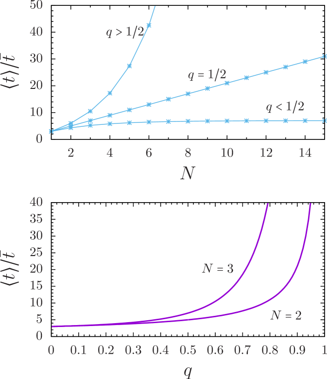
In Fig. 3, we plot the effective mean waiting at a node of the backbone dynamics versus and . It shows that the mean waiting time is a monotonically increasing function of both and . If the random walk inside the branches is isotropic, , one obtains by the L’Hopital’s rule from (26)
| (27) |
To determine the diffusion coefficient for diffusion through the comb, we first calculate the MSD. Performing the Fourier-Laplace transform on (1), we obtain
| (28) |
The MSD in Laplace space reads (see, e.g., Metzler and Klafter (2000))
| (29) |
As mentioned in Sec. II, we assume that the motion on the backbone is unbiased and that the walker only jumps to nearest neighbors. This implies that the kernel is given , and we obtain from (29),
| (30) |
in the large time limit. If the waiting time PDF possesses a finite first moment, (25) implies that the MSD along the backbone corresponds to normal diffusion . The diffusion coefficient is given by
| (31) |
In Fig. 4, we compare the results provided by (31) with numerical simulations.
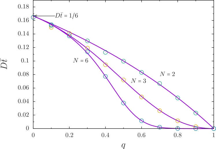
As Fig. 3 demonstrates, increases monotonically with for and saturates at for . Consequently, the mean waiting time is finite for ; the overall diffusion along the backbone is normal. However, for , the mean waiting time increases without bound as increases, and anomalous transport is expected for .
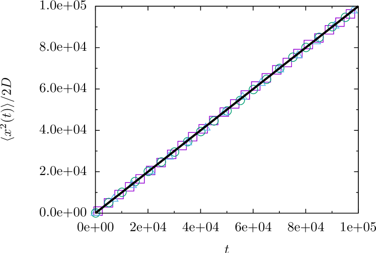
In Fig. 5, we plot the MSD scaled by the diffusion coefficient. It illustrates the result given by (31) for the MSD. The transport is diffusive for finite , regardless and the specific form of , as long as it has finite moments.
We consider now a an effective waiting time PDF with the large-time limit , with Laplace transform and , which does not possess finite moments. Here is a parameter with units of time. In this case, the waiting time PDF for the backbone dynamics is obtained by simply replacing with , i.e, . Substituting this result into (30), we find
| (32) |
for large , where is given by (26), with instead of . If the waiting time PDF at each node of the comb has a power-law tail, then the overall transport along the backbone is anomalous.
III.2
If the number of nodes of the branches goes to infinity, the mean time spent by the walker visiting a branch increases monotonically, see (26). However, this does not always results in anomalous transport along the overall structure as we show below.
For , the quotient and also . We obtain from (21),
| (33) |
where we define for convenience. Equation (24) reduces to
| (34) |
We take the limit and consider first the case where has finite moments. Then , as . The square root in (34) reads
| (35) |
and (34) implies that the waiting time PDF is given by
| (36) |
Substituting (36) into (30), we find for large ,
| (37) |
where the rate of saturation is
| (38) |
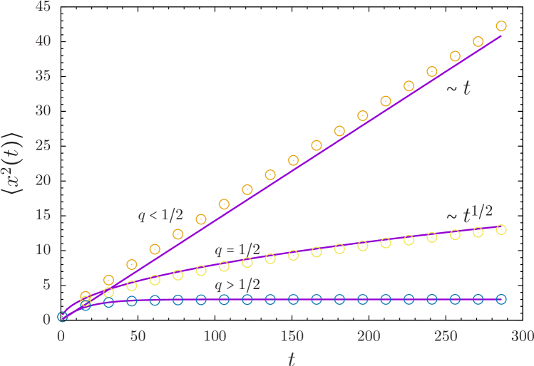
In Fig 6 we compare these results with numerical simulations for . For , we obtain the well known result of subdiffusive transport with the MSD . However, for , the side branches experience advection, and the transport is remarkably different. Namely, for the advection is away from the backbone along the branches, . The walker is effectively trapped inside the branches, and stochastic localization (diffusion failure) occurs, , Denisov and Horsthemke (2000). For , the advection is towards the backbone. It enhances the backbone dynamics and normal diffusion takes place.
Consider now the case where the local waiting time PDF is , i.e., with , as . The MSD in this case can be obtained straightforwardly by replacing with in (36). For large times it reads
| (39) |
where
| (40) |
is expressed in terms of the the generalized Mittag-Leffler function . We use the following property of integration of the Mittag-Leffler function Podlubny (1999),
| (41) |
Subdiffusion in the branches results in backbone subdiffusion for . For advection away from the backbone, , we again find stochastic localization. For , Bateman (1953), and consequently approaches a finite value as .
IV Conclusion
We have developed a mesoscopic equation for a random walk on a regular comb structure given by (2) and (24). The random walk along the branches consists of, possibly biased, jumps to the nearest node, while waiting at each node for a random time distributed according to the PDF before proceeding with the next jump. The overall dynamics along the branches has been reduced to an effective waiting time PDF, given by (24), for motion solely along the backbone. We have obtained statistical properties, such as the effective mean waiting time, for the backbone nodes, and the diffusion coefficient, , of the overall structure for the case where the number of nodes of the branches is finite or infinite. If is finite and has finite moments, both and are derived exactly in terms of the bias probability , the number of nodes on the branch, and the mean waiting time probability at each node. In this case the transport is always normal diffusion. If for large time, it does not posses finite moments and the MSD of the random walker behaves like . If is infinite, the value of is decisive. If has finite moments, the diffusion regime is normal if , while the MSD behaves like for . If , the MSD approaches a constant finite value for large time, corresponding to stochastic localization (diffusion failure). If for large time, the MSD behaves like for and like for Again, stochastic localization occurs for . In summary, if the bias probability of moving away from the backbone is , then stochastic localization occurs, regardless of the other characteristic parameters related to the random walk on the branches.
Acknowledgments
A.I. would like to thank the Universitat Autònoma de Barcelona for hospitality and financial support, as well as the support by the Israel Science Foundation (ISF-1028). VM and DC have been supported by the Ministerio de Ciencia e Innovación under Grant No. FIS2012-32334. VM also thanks the Isaac Newton Institute for Mathematical Sciences, Cambridge, for support and hospitality during the CGP programme where part of this work was undertaken.
References
- Montroll and Shlesinger (1984) E. W. Montroll and M. F. Shlesinger, in Nonequilibrium Phenomena II: From Stochastics to Hydrodynamics, edited by J. L. Lebowitz and E. W. Montroll (Elsevier Science Publishers BV, Amsterdam, 1984), pp. 1–121.
- Metzler and Klafter (2000) R. Metzler and J. Klafter, Phys. Rep. 339, 1 (2000), URL http://dx.doi.org/10.1016/S0370-1573(00)00070-3.
- Klafter and Sokolov (2011) J. Klafter and I. M. Sokolov, First Steps in Random Walks: From Tools to Applications (Oxford University Press, New York, 2011), URL https://global.oup.com/academic/product/first-steps-in-random-walks-9780199234868?cc=us&lang=en&.
- Metzler and Klafter (2004) R. Metzler and J. Klafter, J. Phys. A: Math. Gen. 37, R161 (2004), URL http://dx.doi.org/10.1088/0305-4470/37/31/R01.
- Maex et al. (2003) K. Maex, M. R. Baklanov, D. Shamiryan, F. lacopi, S. H. Brongersma, and Z. S. Yanovitskaya, J. Appl. Phys. 93, 8793 (2003), URL http://dx.doi.org/10.1063/1.1567460.
- Casassa and Berry (1966) E. F. Casassa and G. C. Berry, J. Polymer Sci. A 4, 881 (1966), URL http://dx.doi.org/10.1002/pol.1966.160040605.
- Douglas et al. (1990) J. F. Douglas, J. Roovers, and K. F. Freed, Macromolecules 23, 4168 (1990), URL http://dx.doi.org/10.1021/ma00220a022.
- Frauenrath (2005) H. Frauenrath, Prog. Polymer Sci. 30, 325 (2005), URL http://www.sciencedirect.com/science/article/pii/S0079670005000110.
- Sokolov (2012) I. M. Sokolov, Soft Matter 8, 9043 (2012), URL http://dx.doi.org/10.1039/C2SM25701G.
- White and Barma (1984) S. R. White and M. Barma, J. Phys. A: Math. Gen. 17, 2995 (1984), URL http://stacks.iop.org/0305-4470/17/i=15/a=017.
- Weiss and Havlin (1986) G. H. Weiss and S. Havlin, Physica A 134, 474 (1986), URL http://dx.doi.org/10.1016/0378-4371(86)90060-9.
- Arkhincheev and Baskin (1991) V. Arkhincheev and E. Baskin, Sov. Phys. JETP 73, 161 (1991), URL http://jetp.ac.ru/cgi-bin/dn/e_073_01_0161.pdf.
- Méndez and Iomin (2013) V. Méndez and A. Iomin, Chaos, Solitons & Fractals 53, 46 (2013), URL http://www.sciencedirect.com/science/article/pii/S0960077913000830.
- Iomin and Méndez (2013) A. Iomin and V. Méndez, Phys. Rev. E 88, 012706 (2013), URL http://link.aps.org/doi/10.1103/PhysRevE.88.012706.
- Marsh et al. (2008) R. E. Marsh, T. A. Riauka, and S. A. McQuarrie, Q. J. Nucl. Med. Mol. Imaging 52, 278 (2008), URL http://www.minervamedica.it/index2.t?show=R39Y2008N03A0278.
- Arkhincheev et al. (2011) V. E. Arkhincheev, E. Kunnen, and M. R. Baklanov, Microelectron. Eng. 88, 694 (2011), URL http://dx.doi.org/10.1016/j.mee.2010.08.028.
- Stanley and Coniglio (1984) H. E. Stanley and A. Coniglio, Phys. Rev. B 29, 522 (1984), URL http://link.aps.org/doi/10.1103/PhysRevB.29.522.
- Tarasenko and Jastrab´ık (2012) A. Tarasenko and L. Jastrabík, Microporous and Mesoporous Materials 152, 134 (2012), URL http://www.sciencedirect.com/science/article/pii/S1387181111005725.
- Hannunen (2002) S. Hannunen, Ecol. Model. 155, 149 (2002), URL http://www.sciencedirect.com/science/article/pii/S0304380002001254.
- Agliari et al. (2014) E. Agliari, A. Blumen, and D. Cassi, Phys. Rev. E 89, 052147 (2014), URL http://link.aps.org/doi/10.1103/PhysRevE.89.052147.
- Rebenshtok and Barkai (2013) A. Rebenshtok and E. Barkai, Phys. Rev. E 88, 052126 (2013), URL http://link.aps.org/doi/10.1103/PhysRevE.88.052126.
- Forte et al. (2013) G. Forte, R. Burioni, F. Cecconi, and A. Vulpiani, J. Phys.: Condens. Matter 25, 465106 (2013), URL http://stacks.iop.org/0953-8984/25/i=46/a=465106.
- Korabel and Barkai (2010) N. Korabel and E. Barkai, Phys. Rev. Lett. 104, 170603 (2010), URL http://link.aps.org/doi/10.1103/PhysRevLett.104.170603.
- Baskin and Iomin (2004) E. Baskin and A. Iomin, Phys. Rev. Lett. 93, 120603 (2004), URL http://dx.doi.org/10.1103/PhysRevLett.93.120603.
- Iomin and Baskin (2005) A. Iomin and E. Baskin, Phys. Rev. E 71, 061101 (2005), URL http://dx.doi.org/10.1103/PhysRevE.71.061101.
- Van den Broeck (1989) C. Van den Broeck, Phys. Rev. Lett. 62, 1421 (1989), URL http://link.aps.org/abstract/PRL/v62/p1421.
- Campos and Méndez (2005) D. Campos and V. Méndez, Phys. Rev. E 71, 051104 (2005), URL http://dx.doi.org/10.1103/PhysRevE.71.051104.
- Campos et al. (2006) D. Campos, J. Fort, and V. Méndez, Theor. Pop. Biol. 69, 88 (2006), URL http://dx.doi.org/10.1016/j.tpb.2005.09.001.
- Kahng and Redner (1989) B. Kahng and S. Redner, J. Phys. A: Math. Gen. 22, 887 (1989), URL http://stacks.iop.org/0305-4470/22/i=7/a=019.
- Denisov and Horsthemke (2000) S. I. Denisov and W. Horsthemke, Phys. Rev. E 62, 7729 (2000), URL http://dx.doi.org/10.1103/PhysRevE.62.7729.
- Podlubny (1999) I. Podlubny, Fractional Differential Equations (Academic Press, San Diego, 1999).
- Bateman (1953) H. Bateman, Higher Transcendental Functions [Volumes I-III] (McGraw-Hill, New York, 1953), URL http://resolver.caltech.edu/CaltechAUTHORS:20140123-104529738.