Meta-analysis of photometric and asteroseismic
measurements
of stellar rotation periods:
the Lomb-Scargle periodogram, autocorrelation
function, wavelet and rotational splitting analysis for 92 Kepler asteroseismic targets
Abstract
We perform intensity variability analyses (photometric analyses: the Lomb-Scargle periodogram, autocorrelation, and wavelet) and asteroseismic analysis of 92 Kepler solar-like main-sequence stars to understand the reliability of the measured stellar rotation periods. We focus on the 70 stars without reported stellar companions, and classify them into four groups according to the quarter-to-quarter variance of the Lomb-Scargle period and the precision of the asteroseismic period. We present detailed individual comparison among photometric and asteroseismic constraints for these stars. We find that most of our targets exhibit significant quarter-to-quarter variances in the photometric periods, suggesting that the photometrically estimated period should be regarded as a simplified characterization of the true stellar rotation period, especially under the presence of the latitudinal differential rotation. On the other hand, there are a fraction of stars with a relatively small quarter-to-quarter variance in the photometric periods, most of which have consistent values for asteroseismically and photometrically estimated rotation periods. We also identify over ten stars whose photometric and asteroseismic periods significantly disagree, which would be potentially interesting targets for further individual investigations.
1 Introduction
Observational studies of stellar rotation play a fundamental role in understanding the physics of stars. The rotation rate of stars evolves substantially over their main-sequence stage due to a variety of angular momentum loss processes. Various empirical relations between the period, age and mass have been derived, known as gyrochronology (e.g. Skumanich, 1972; García et al., 2014; van Saders et al., 2016). The determination of rotation periods for a large number of stars with different masses and ages is critical for verifying and understanding the physics behind these relations. In reality, stars are supposed to exhibit latitudinal and internal radial differential rotation. Thus the observed stellar rotation period is not a unique quantity, but should be interpreted as a weighted average dependent on specific observational methods.
Indeed, the rotation period of the Sun is known to vary along both latitudinal (via spectroscopy, e.g. Howard & Harvey, 1970) and radial (via helioseismology, e.g. Schou et al., 1998) directions. The internal radiative core of the Sun () is well-approximated by a solid body rotation of days. In contrast, beyond the transition region between the radiative and outer convective zones at (so-called tachocline), the rotation period becomes significantly dependent on the latitude (Thompson et al., 2003), varying from days () to days ().
Such detailed rotational profiles, however, are poorly understood for other solar-like stars except the Sun. Furthermore, the Sun shows a magnetic activity cycle of 11-years, that is thought to be related to near-surface convection and stellar rotation (e.g. Thompson et al., 2003; Hartmann & Noyes, 1987). Due to this link, the large range of activity observed among stars suggest caution when interpreting the measures of rotation periods.
With the high precision photometry from Kepler and TESS, measurements of stellar rotation periods have been significantly improved in both quantity and accuracy. Since the starspots over the stellar surface are mainly responsible for the variation of stellar light intensity, the surface rotation period may be inferred from the intensity variability analyses using the Lomb-Scargle periodogram (e.g. Nielsen et al., 2013), auto-correlation function (ACF, e.g. McQuillan et al., 2013, 2014) and wavelet analysis (e.g. García et al., 2014; Ceillier et al., 2016).
Note that those photometric measurements are sensitive to the observed distribution of spots on the stellar surface. The number of spots varies in a time-dependent manner due to the continuous creation and annihilation processes, and those spots spread over a range of different latitudes. All of them inevitably complicate the correspondence between the observed photometric variation and the stellar rotation in particular due to the stellar differential rotation. Furthermore, the photometric variation is produced solely by those spots located at the range of latitudes on the hemisphere visible to the observer. Thus, the measured rotation periods should depend on both the stellar inclination relative to the observer’s line-of-sight and the non-stationary latitudes of the visible spots as discussed in detail by Suto et al. (2022).
Spectroscopic data of the stellar lines measure the projected rotation velocity . If additional information for the stellar radius and inclination is available, it also provides an independent estimate for the stellar rotation period; further discussion is given in Kamiaka et al. (e.g. 2018).
Yet another complementary estimate for the stellar rotation period can be derived from asteroseismic analysis, which models the stellar oscillation pattern in power spectrum (e.g. Kjeldsen & Bedding, 1995; Gizon & Solanki, 2004; Appourchaux et al., 2008; Kamiaka et al., 2018; García et al., 2019). Unlike the the photometric variation of the stellar light curves, asteroseismic analysis estimates the averaged rotation period over a range of stellar latitude and radius. In this sense, the stellar rotation periods estimated with the two complementary methods do not have to be identical, depending on the degree of the differential rotation. In turn, the comparison of the two results for a sample of stars puts interesting constraints on the differential rotation, if the reliability of both measurements is confirmed.
It should be noted that the rotation profile of stars has been investigated using the high-quality photometry. Reinhold & Gizon (2015) attempted to detect surface differential rotation by studying significant peaks in the Lomb-Scargle periodogram for more than ten thousand Kepler stars. In addition, Benomar et al. (2018) measured the latitudinal differential rotation in the convection zones for 40 Sun-like stars by asteroseismology.
In this paper, we compute the rotation periods using three independent photometric methods (i.e., intensity variability analyses using the Lomb-Scargle periodogram, auto-correlation function, and wavelet) for 92 Kepler Sun-like stars, which were selected as targets for asteroseismic analysis by Kamiaka et al. (2018). The present paper performs systematic and complementary analyses of the intensity variability of the same stars, and compares the different methods for measuring the stellar rotation periods. The detailed comparison against their asteroseimically determined rotation periods by Kamiaka et al. (2018) enables us to understand the reliability and possible biases of the rotation periods measured from different methods on an individual basis.
Nielsen et al. (2015) compared the rotation periods derived from the Lomb-Scargle and asteroseismic analyses, and , for their six Sun-like target stars, and found that they agree within the measurement uncertainty. We expand the sample size to 92 Kepler solar-type stars, and compute the stellar rotation period from three photometric methods. The reliability of such photometric rotation periods can be tested through the agreement among the three independent methods, while their variation in different quarters over four years may probe the latitudinal differential rotation as proposed by Suto et al. (2022). In addition, comparison against the asteroseismic estimates of the rotation periods may constrain the stellar inclination (Kamiaka et al., 2018, 2019; Suto et al., 2019). Thus, the result enables us to evaluate the reliability of the measurements, as well as to extract the possible signature of, and/or put constraints on, their differential rotations.
The rest of the paper is organized as follows. Section 2 presents our sample of 92 Sun-like stars selected from the Kepler data, and the flow of our data processing. We identify 22 possible binary/multiple star systems. In section 3, we classify the remaining 70 stars into four groups according to the variance of the photometric rotation periods from the Lomb-Scargle analysis in different quarters, and the fractional uncertainties in the asteroseismic periods. Section 4 compares photometric and asteroseismic rotation periods for the 70 stars individually, while their statistical comparison among photometric analyses and between photometric and asteroseismic results is given in sections 5 and 6, respectively. Section 7 presents implications of our results. Finally, section 8 is devoted to summary and conclusions of the paper. In appendix, we describe our methods to estimate the rotation period, various comparison against previous results, the Lomb-Scargle periodograms and asteroseismic constraints for potentially interesting stars that are mentioned in the main text.
2 Our sample and data processing of light curves
2.1 Our sample of stars
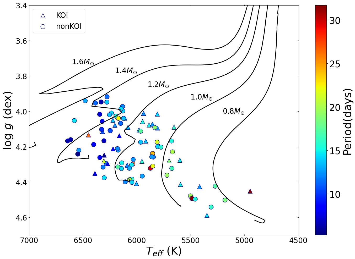
We use the sample of stars selected by Kamiaka et al. (2018). The sample includes the Kepler dwarfs LEGACY sample which consists of 66 stars with the best asteroseismic data so far in solar-type category (see e.g. Lund et al., 2017; Aguirre et al., 2017), and additional 28 KOI (Kepler Object of Interest) with detectable oscillation amplitudes. The Kepler targets in the LEGACY sample have magnitudes around 9, which are in general brighter than those for the KOI sample (Kepler magnitude around 11). Thus, the LEGACY sample has spectra with higher height to background ratio and hence their periods can be estimated more precisely. The additional 28 KOI targets are useful to examine whether the stellar inclinations are correlated to the orbital axis of their transiting planets. Kamiaka et al. (2018) performed an asteroseismic analysis of this sample, and estimated their stellar rotation periods and inclinations. Figure 1 plots the location of our targets on their surface gravity and effective temperature plane. Stellar evolutionary tracks are computed with MESA code (Modules for Experiments in Stellar Astrophysics; Paxton et al. (2011)) for stars with initial mass of 0.8, 1.0, 1.2, 1.4, and 1.6 from their pre-main-sequence phase to white dwarf phase, assuming the solar metallicity.
For the photometric analysis, we use the Kepler long-cadence PDC light curve (PDC-msMAP, Stumpe et al., 2014), Data Release 25, from Mikulski Archive for Space Telescope (MAST). The data consist of quarters of day duration with a cadence of minutes over four years. We choose the light curves for Q2-Q14 quarters.
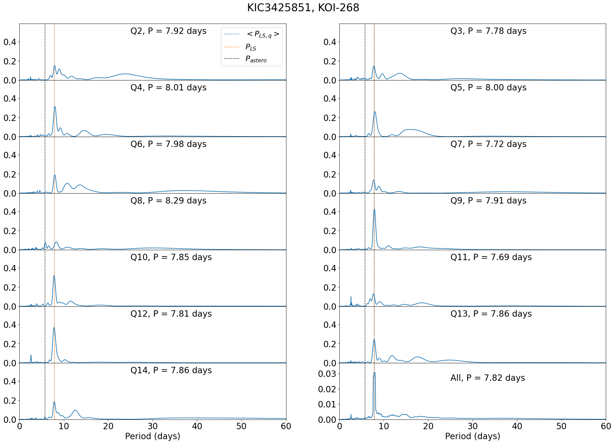
KOI-268 (KIC 3425851) has one of the best-quality light curves in our sample and a precisely determined photometric period (see Figures 4 and 44 below). We first compute the duty cycle for KOI-268 in each quarter, and find that it varies between 81 and 96 percents, with an average 90 percents. Then, we remove those quarters for other stars if the duty cycle is less than of the reference value for KOI-268, in order to secure the statistical significance of each quarter. Furthermore, we require that the targets must have at least 7 quarters of available data, which removes 16 Cyg A (KIC 12069424) and 16 Cyg B (KIC 12069449) from our sample. Thus, the number of our final targets for subsequent analyses becomes 92.
2.2 Preprocessing stellar light curves
We preprocess the light curves of the 92 stars before performing the photometric analysis, which is summarized in Figure 2.

In order to remove the systematic trend in the light curves, we first fit the original data in each quarter to a 4-th order polynomial function . Then, we obtain the detrended light curves in units of the fitted polynomials separately in each quarter: (Step 1 of Figure 2). In order to remove a long-term trend in a light curves, it is fairly common to fit using polynomials. We make sure that detrending with a third-order or fourth-order polynomials does not change the estimate of the rotation periods unless they are longer than days. Since the duration of each quarter is 90 days and the Kepler instrument performs pointing corrections every 30 days which are known to generate a recurrent noise around that period, periods longer than days are not reliable in any case. Therefore, we decide to use the fourth polynomials in detrending.
Next, we concatenate the detrended light curves in available quarters between Q2 and Q14 for each target star into a single array of time series while preserving gaps between the quarters (Step 2 of Figure 2). We set the starting time of this series to be .
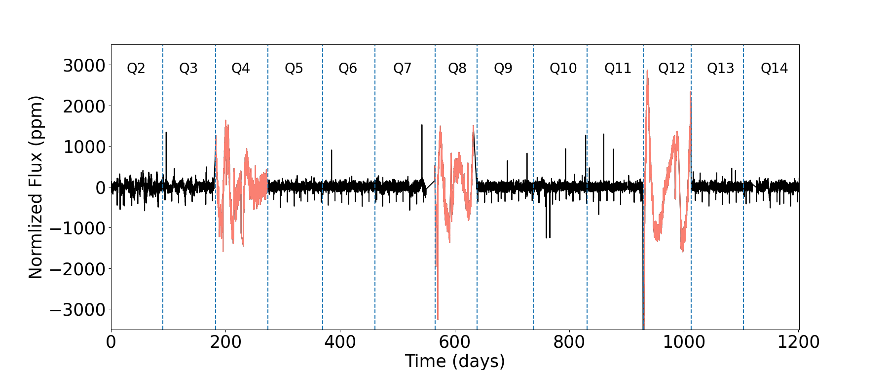
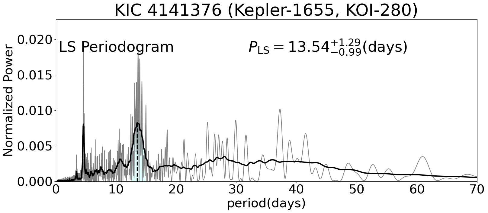
For several stars, the detrended light curves still exhibit large anomalous variations in some quarters. Figure 3 illustrates such an example for Kepler-1655 (KIC 4141376, KOI-280). The light curves in quarters Q4, Q8, and Q12 (plotted in red) show strange behavior that seems to be uncorrelated with nearby quarters. We suspect that they are due to unknown contamination or instrumental effects. Thus, we decided to remove those quarters if the median absolute flux variation in a particular quarter is three times larger than those of the neighboring quarters. We removed such anomalous quarters from six targets: Kepler-1655 (KIC 4141376, KOI-280), Kepler-100 (KIC 6521045), Kepler-409 (KIC 9955598, KOI-1925), KOI-72 (KIC 11904151), KIC 8694723, and KIC 10730618.
As shown in Figure 3, the detrended light curves also contain the dips due to the planetary transits (for KOI stars) and other possible outliers. We remove them according to the following procedure (Steps 3 and 4 of Figure 2).
In order to remove the periodic dips due to the planetary transit, we first fold the light curves of the KOI sample according to the orbital period of the planet candidates. Then we remove the data corresponding to the transit and occultation phases. The occulations might not be visible for all targets. For those targets we remove the expected occultations by assuming a circular orbit. The duration of transits and occultations is of the order of hours as opposed to the orbital period of the order of days. Thus, the amount of data removed is relatively negligible, and does not change the estimate of the stellar rotation period in practice. In addition, we remove the other outliers by -clipping with a threshold of and the center value being the median of concatenated light curve. The data removed in this step is less than 1%, and thus do not affect the period estimation either.
Incidentally, we are not able to detect the transit signal for KOI-5.02 and Kepler-37b after folding, and we do not remove any transit dips nor the expected eclipse dips. We suspect that KOI-5.02 is a false-positive, and Barclay et al. (2013) reported that the transit signal of Kepler-37b is less than 20 ppm. Thus possible transiting signals of these two targets would have negligible influence on the determination of stellar rotation period.
We note that the 90 day duration of each Kepler quarter effectively puts an upper limit of detectable periods around 45 days. Indeed, the rotation periods of main-sequence stars similar to our sample (Figure 1) are usually less than 50 days (e.g. Kamiaka et al., 2018). So, we apply our own box-car filter of a 50-day width even though the PDC-SAP light curves has applied smoothing to reduce long-term period systematics. Since the Kepler data is nearly evenly sampled, we map the light curve to a uniformly sampled grid at an interval of minutes.
Finally, we pad all removed portions in the light curves (removed quarters, planetary transits, secondary eclipses, outliers, and missing data) by Gaussian noise of zero mean and the variance of that is computed from the detrended light curve for each target (Step 5 of Figure 2). We also tried the zero padding for comparison, and made sure that the two padding schemes hardly change the estimated values of the photometric rotation period, implying that the padding does not affect the result in reality.
2.3 Identification of Possible Binary/Multiple-star Systems
A significant fraction of stars are in multiple systems. The multiplicity may lead to a systematic bias on the rotation period estimated from the photometric variation of the target star. Thus, we try to identify possible members in binary and multiple-star systems in our sample.
For that purpose, we primarily adopt Renormalized Unit Weight Error (RUWE) value from Gaia DR3, which measures the goodness of fit with respect to a single-star model derived from the Gaia astrometry (Fabricius et al., 2021). A star with RUWE exceeding 1.4 is commonly suspected to have an unresolved companion(Evans, 2018; Wolniewicz et al., 2021). We list 14 target stars with RUWE from the Gaia DR3 catalog as possible candidates of binary/multiple-star systems.
In addition, we identify three eclipsing binaries from Kepler Eclipsing Binary Catalogue (Kepler Eclipsing Binary working group, 2019), two binary systems from NASA Exoplanet Archive (Kepler Mission, 2019), four multiple-star systems and two binaries from Table 4 of García et al. (2014), one binary from Eylen et al. (2014), and one binary from Lillo-Box et al. (2014). Among the 13 systems, five stars have RUWE , while the other eight stars have RUWE .
In total, we identify 22 stars with possible companions, and summarize them in Table 2. We compute their photometric rotation periods in the same manner as other 70 stars with no reported stellar companion (Appendix A), but they may be interpreted with caution. We separately discuss seven KOI stars out of them in §7.2 since they may be potentially important targets for planetary studies. In what follows, however, we mainly focus on the other 70 stars; their estimated rotation periods are summarized in Tables 3, 4, 5 and 6.
3 Classification of stars
We measure rotation periods using three different photometric methods, including the Lomb-Scargle (LS) periodogram, Auto-correlation function (ACF) and wavelet analysis (WA). The details of the photometric methods as well as a brief introduction to the asteroseismic analysis by Kamiaka et al. (2018) are provided in Appendix A. In this section, we classify the 70 stars based on photometric and asteroseismic results, in order to examine the reliability of the measured rotation period and/or to constrain the differential rotation. We adopt the LS measurement for the photometric classification, and use ACF and WA as complementary information to test the robustness of the derived rotation period.
3.1 Photometric classification based on the variance of rotation periods in different quarters
The rotation period estimated using the LS method for the -th quarter may be different from the period computed for the entire observed duration . Distribution of starspots at different quarters should change with time due to the creation/annihilation processes over a range of latitudes. Thus, combined with their possible latitudinal differential rotation, each quarter may exhibit the fractional variation of the period on the order of ten percent.
If the typical lifetime of starspots is less than days, their pattern on the surface at different quarters can be regarded as an uncorrelated realization drawn from the same statistical distribution. Even if the lifetime of starspots has a broad distribution, the variance of among different quarters would reflect the differential rotation for stars. This possibility has been theoretically studied by Suto et al. (2022) using analytic model and mock observations. It is also possible that the large variance is simply due to the low signal-to-noise ratio (e.g., due to a very low number of spots or to the fact that the star is very faint) of the light curve for some quarters. These two possibilities could be distinguished by comparing the LS result with those based on ACF, WA, and asteroseismology on an individual basis (see §3.2 below).
In order to quantify the fractional variance of the rotation periods among different quarters, we introduce the following parameter for each star:
| (1) |
where is the number of quarters with measured , and denotes the median value operator.
Nielsen et al. (2013) proposed a similar indicator called MAD (Median Absolute Deviation) . Our indicator, equation (1), differs from MAD in the following two ways. We use the fractional variance, which would be more appropriate in classifying stars with a broad range of rotation periods. In addition, we average the deviation over all the quarters because the median of deviation sometimes underestimates the real intrinsic variation of the distribution. This will be discussed below individually for each target.
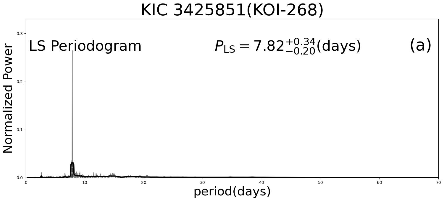
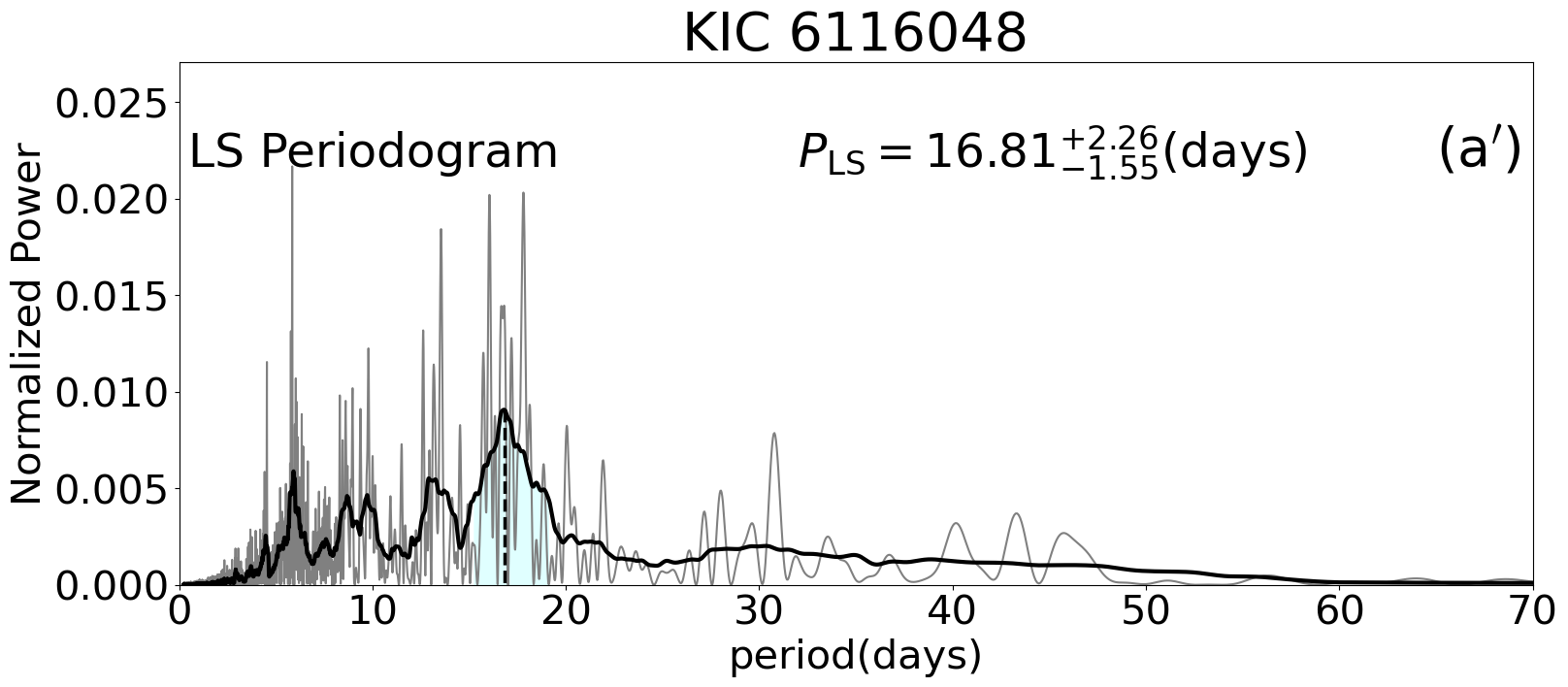
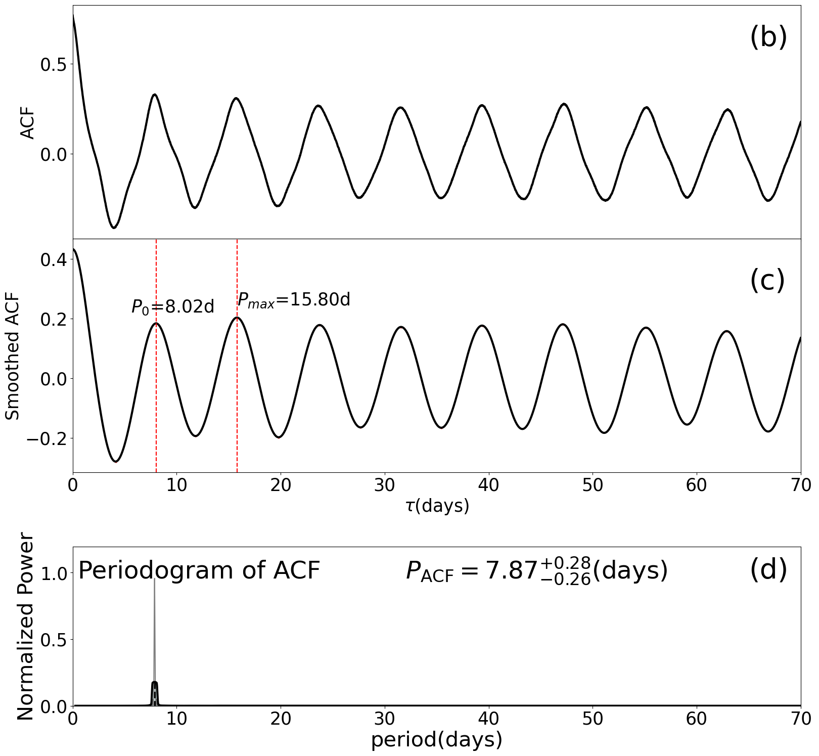
After trial-and-errors, we classify the stars into two groups: Group A with and Group B with . To select the threshold, we first plot the rotation period against , and find that a group of targets with 30 days and significantly large error-bars start to occur from . Thus, we decide to set a threshold of = 0.2 for a reliable group just for convenience. There are 23 stars in Group A and 47 stars in Group B, out of the 70 stars with no reported stellar companion; see §2.3. Figure 4 presents results of our photometric analysis for the reference star KOI-268 (KIC 3425851; see section 2) that is classified in Group A with , as well as for KIC 6116048 (Group B with ).
Group A contains targets with a relatively robust periodic component in their light curves, and their values are reliably estimated from the prominent single peak as shown in the left panels of Figure 4.
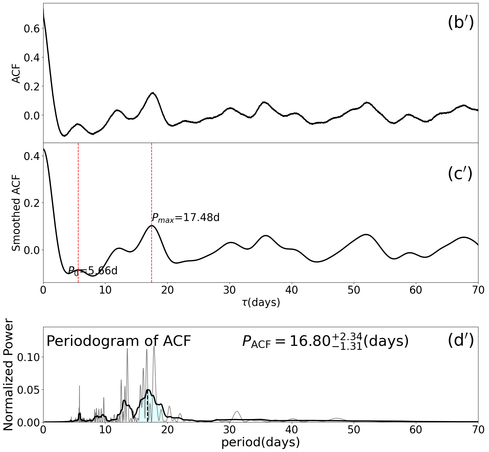
In contrast, Group B, with , consists of two different types in general. The first type shows either a variation of measured periods among different quarters or multiple co-existing periodic signals (see e.g., the right panels of Figure 4). Possible scenarios for the latter include differential rotation on stellar surface, harmonics (see §A.1.1), unresolved companions, residuals of a systematic trend, and other unknown contaminations. The second type shows very weak periodic signals, whose estimated periods are less reliable and subject to significant uncertainties.
Note that the large variation of period measurements for the first type of targets in Group B may not necessarily indicate that their rotation periods are unreliable, but could be due to the physical variation on stellar surface such as the differential rotation.
3.2 Classification based on asteroseismic analysis
We also classify our targets based on asteroseismically estimated periods by Kamiaka et al. (2018), in a complementary manner to the photometric classification. For that purpose, we adopt the ratio , where is the sum of upper and lower error of period estimation, i.e., ; see equations (A7) and (A8) in §A.2.
We set the threshold value of after trial-and-errors, and introduce two groups; Group a with has 33 stars, while Group b with has 37 stars.
| Group | Group | Total | |
|---|---|---|---|
| Group | 14 (7) | 9 (4) | 23 (11) |
| Group | 19 (3) | 28 (12) | 47 (15) |
| Total | 33 (10) | 37 (16) | 70 (26) |
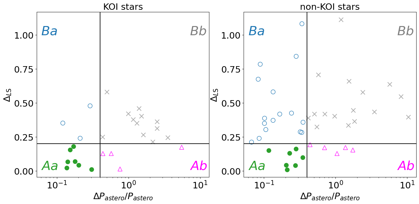
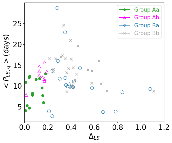
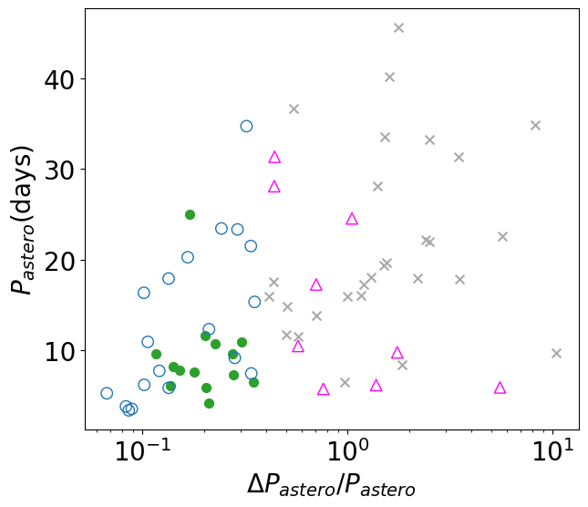
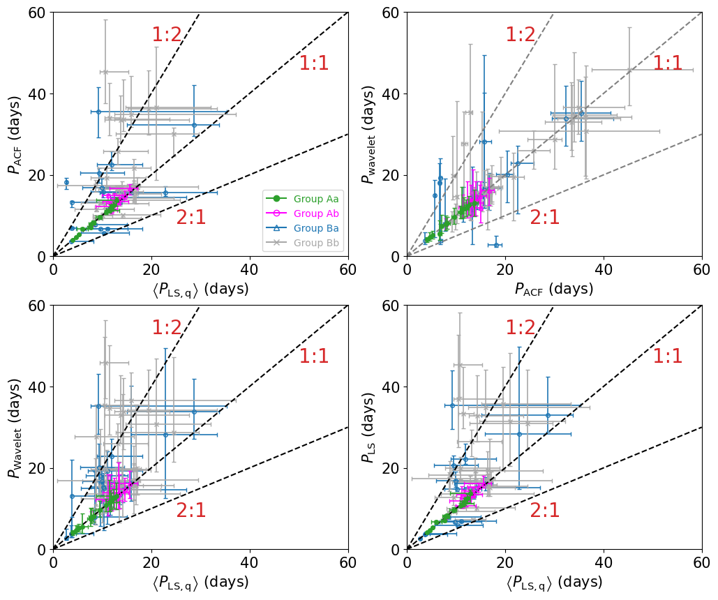
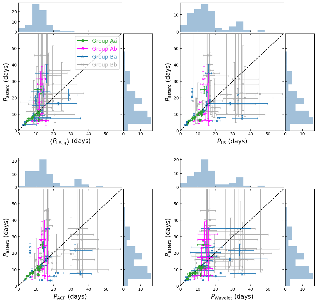
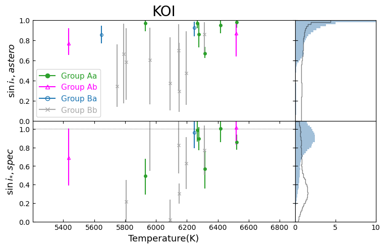
Combining the photometric and asteroseismic classification yields four groups labeled as Aa, Ab, Ba, and Bb, which are summarized in Table 1. Figure 5 plots the locations of 70 stars on the – plane, and the left and right panels of Figure 6 show the correlations between and , and between and , respectively.
4 Remarks on individual stars
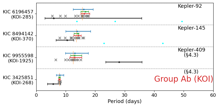
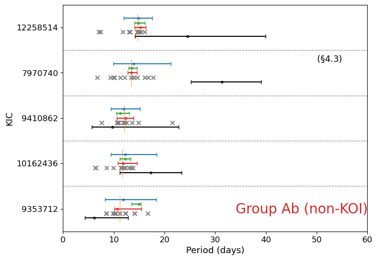
We plot the rotation periods for 70 stars with no obvious stellar companion in Figure 7 (7 KOI stars in Group Aa), Figure 9 (7 non-KOI stars in Group Aa), Figure 10 (4 KOI stars in Group Ab), Figure 11 (5 non-KOI stars in Group Ab), Figure 12 (3 KOI stars in Group Ba), Figure 13 (16 non-KOI stars in Group Ba), Figure 14 (12 KOI stars in Group Bb), and Figure 15 (16 non-KOI stars in Group Bb).
In those figures, gray crosses indicate the values of for different quarters with the orange vertical lines being their median value , while the blue, green, red, and black dots with error-bars represent the values of , , , and with their uncertainties defined in section A. Those values are summarized in appendix; Tables 3 (Group Aa), 4 (Group Ab), 5 (Group Ba), and 6 (Group Bb). In those Tables, we quote the upper and lower error-bars with respect to the median value by introducing
| (2) |
where and denote the median operators for quarters with and , respectively. For a majority of stars, equation (2) gives a very similar value of the Half Width at Half Maximum (HWHM) of the highest peak computed from the LS periodogram over the entire observation span. In some cases, however, it becomes much larger reflecting the significant skewness of the distribution of . We adopt equation (2) as a complementary measure to emphasize the presence of such skewness, which are listed in Tables 3, 4, 5 and 6.
Before considering the statistical comparison and implications, we comment on individual results for a few targets in different groups. In the following discussion, we assume solid rotation for simplicity, and estimate the stellar rotation period from the spectroscopically determined rotation velocity :
| (3) |
and from the asteroseismically determined rotation frequency :
| (4) |
4.1 KOI stars in Group Aa: Kepler-100
As Figure 7 clearly indicates, KOI stars in Group Aa show good agreement among , , , , and . Indeed, the major part of the scatter around for those stars is dominated by a small number of quarters with low signal-to-noise ratios.
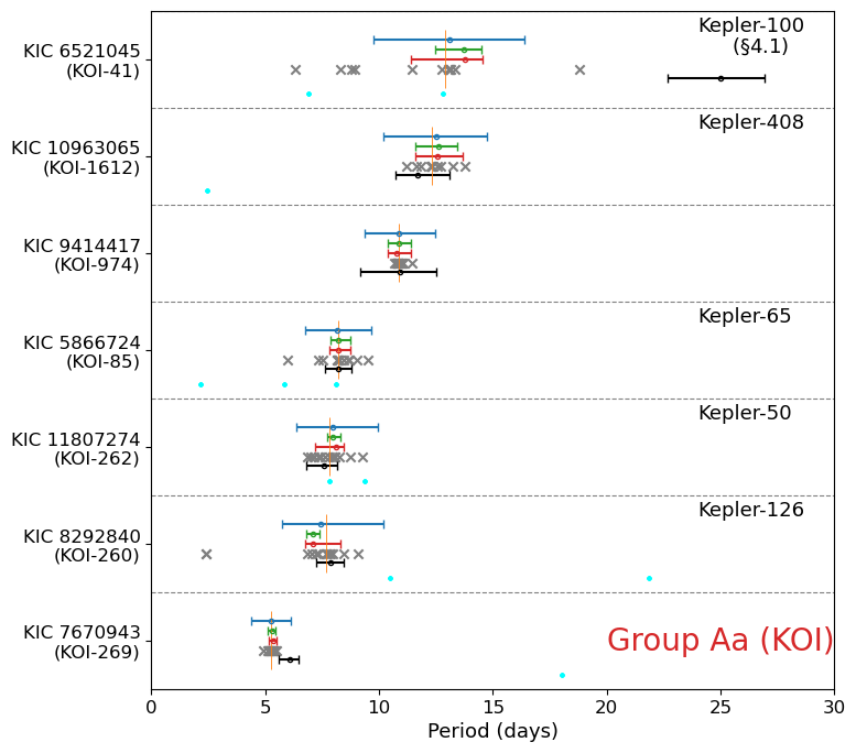
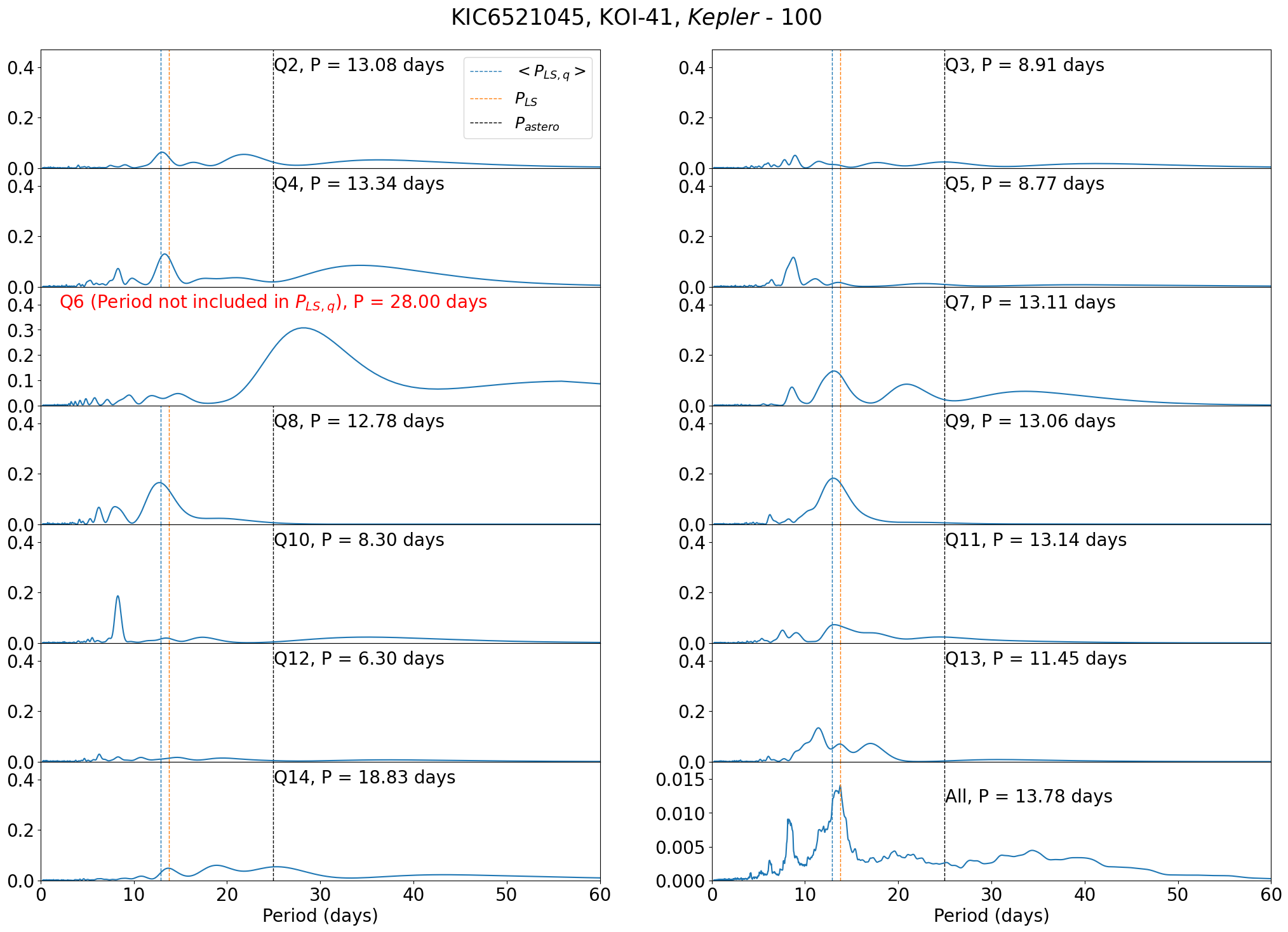
The only exception is Kepler-100 (KIC 6521045, KOI-41) with that is close to our threshold value of 0.2. Its photometrically estimated periods (, , , and ) consistently point to days, while days. Intriguingly, McQuillan et al. (2013) and Ceillier et al. (2016) concluded days. Thus, we conduct a further examination of Kepler-100.
The LS periodograms of Kepler-100 for different quarters (Figure 31) shows apparent variations in measured period. While it is not easy to define a robust period, six quarters (Q2, Q4, Q7, Q8, Q9, Q11) out the 12 quarters (except Q6) have the highest peaks around days. Our analysis excludes Q6 because its median absolute flux variation is more than three times of those of the neighboring quarters (§2.2). Nevertheless, the quarter has a very strong peak at days. We found that our own becomes days if we include the Q6 data, which recovers the result of McQuillan et al. (2013) and Ceillier et al. (2016).
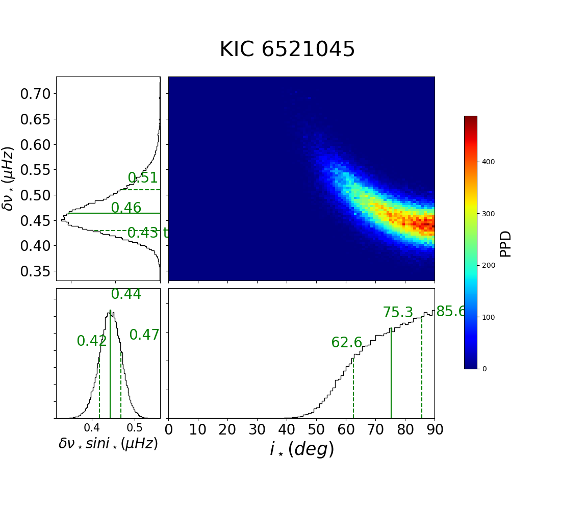
We refer to spectroscopic measurement of rotational velocity. According to Table 1 of Marcy et al. (2014), Kepler-100 have and . Thus equation (3) implies that days. A value of is required to agree with days, but it is inconsistent with the asteroseismic result of and days (Hz; see Figure 31).
We note that the orbital periods of its three transiting planets (Marcy et al., 2014) are days (Kepler-100 b), days (Kepler-100 c), and days (Kepler-100 d), one of which are close to our measured rotation period (13 days). We visual inspect the light curves to check whether our photometric estimate is somehow contaminated by the removal of the transit signal of Kepler-100 b. As Figure 8 suggests, however, the lightcurves exhibit clear periodic oscillations that are not aligned with the location of the transit dip. Therefore, it is unlikely to be an artifact of the transit signal removal. We also confirm that different padding schemes (with and without noise) give consistent measurements of the rotation period.
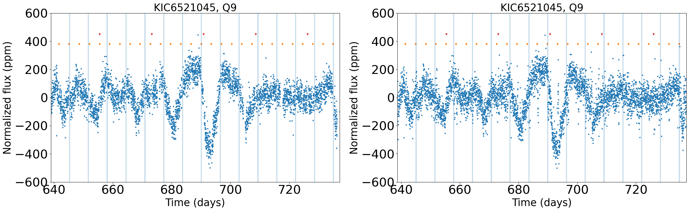
A possible explanation is that the 13-day period is the second harmonics of 25 days. The variation of the period in different quarters may suggest that Kepler-100 has multiple large active spots over the surface. Indeed, our visual inspection of light curve (Figure 8) shows a pattern of a deeper trough accompanied by a shallower trough. This pattern may be a signature of multiple spots, which leads to the presence of the harmonics (peak at /2) in periodogram. Without visual inspection, the automatic period detection method may the period associated with harmonics as the actual rotation period. In any case, we conclude that Kepler-100 remains as one of the intriguing systems that deserve for further investigation.
4.2 non-KOI stars in Group Aa: KIC 5773345
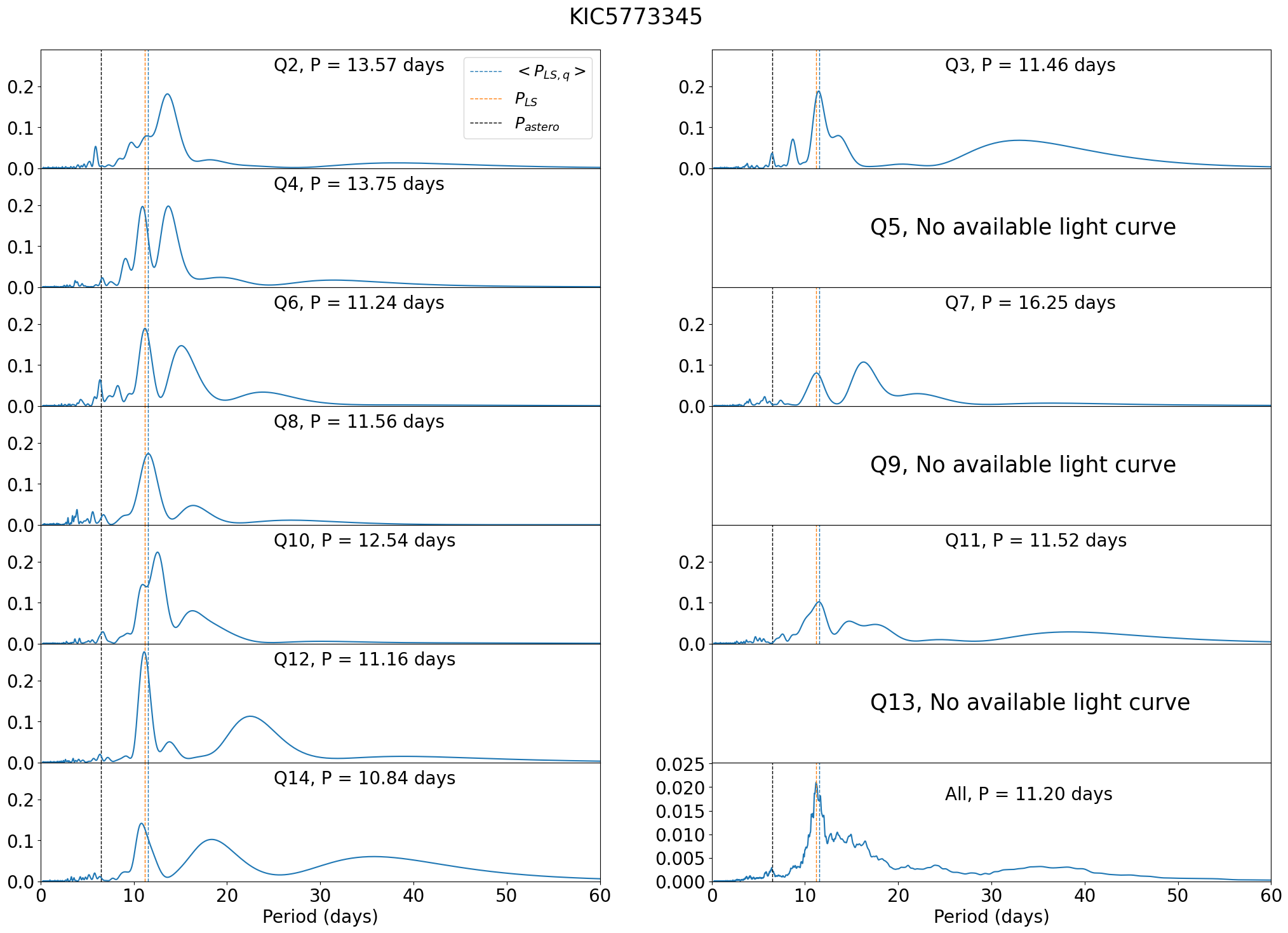
Photometric rotation periods , , , and agree within error-bars for all the non-KOI targets in Figure 9. In contrast, days of KIC 5773345 is a factor of two smaller than the photometrically derived values of days. Thus, we examine KIC 5773345 in detail below.
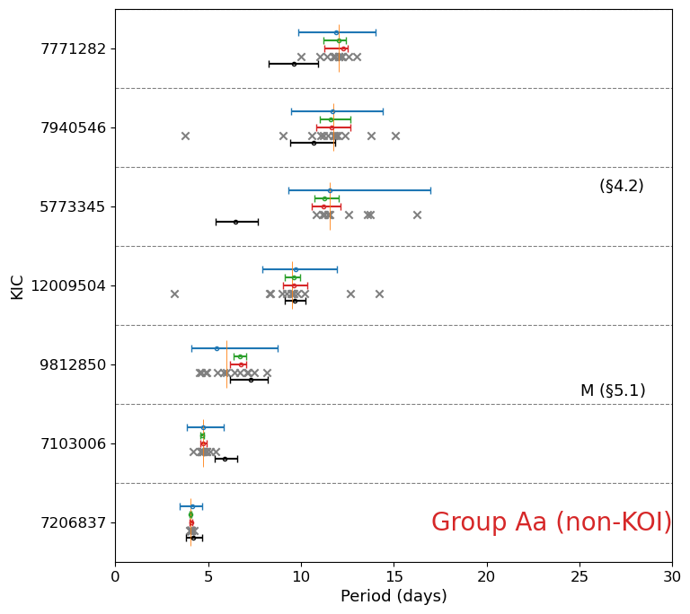
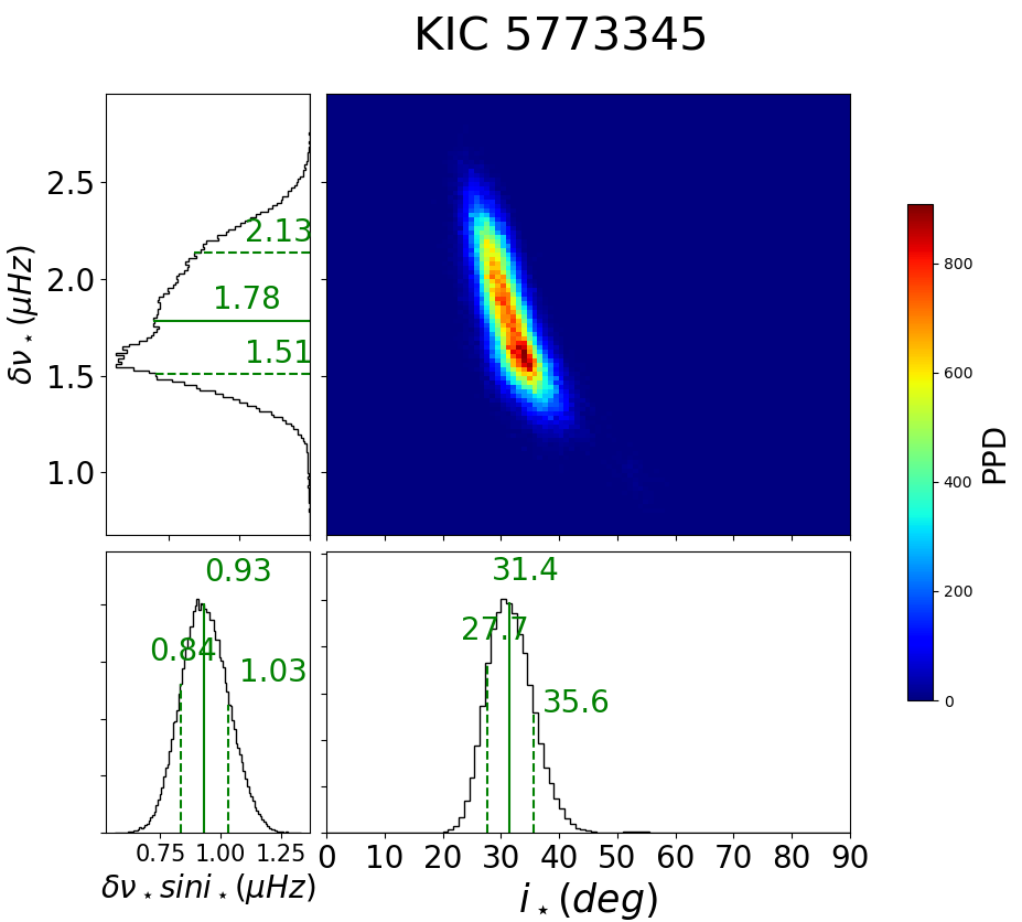
Figure 32 indicate that KIC 5773345 has persistent periodic signals of P days over the entire observed span (except for the removed quarters), while there is no significant signal around days. Asteroseismic constraints on and for KIC 5773345 are shown in Figure 33.
Another complementary constraint on the rotation period is provided from the spectroscopic data. For KIC 5773345, Bruntt et al. (2012) and Molenda-Żakowicz et al. (2013) obtained km/s and km/s, respectively. The factor of two difference likely comes from the difficulty of modeling the turbulence as pointed out by Kamiaka et al. (2018); see their Figure 8. Adopting (Chaplin et al., 2013), equation (3) gives days and days, respectively.
Our photometric estimate of days becomes consistent with of Bruntt et al. (2012) and Molenda-Żakowicz et al. (2013) if and , respectively. Incidentally, it is known that the asteroseismology constrains the parameter primarily, instead of or (Kamiaka et al., 2018). Substituting Hz (Figure 33) into equation (4) implies days, which agrees with the result of Bruntt et al. (2012) within their 1 uncertainty while inconsistent with that of Molenda-Żakowicz et al. (2013).
Therefore, the discrepancy between our photometric and asteroseismic periods for KIC 5773345 may come from a intrinsic problem of asteroseismic analysis in separating into and in asteroseismic analysis. In such case, the photometric estimate of is likely the true rotation period. Nevertheless, it may be premature to conclude at this point, and KIC 5773345 should be regarded as another interesting target for follow-up observation.
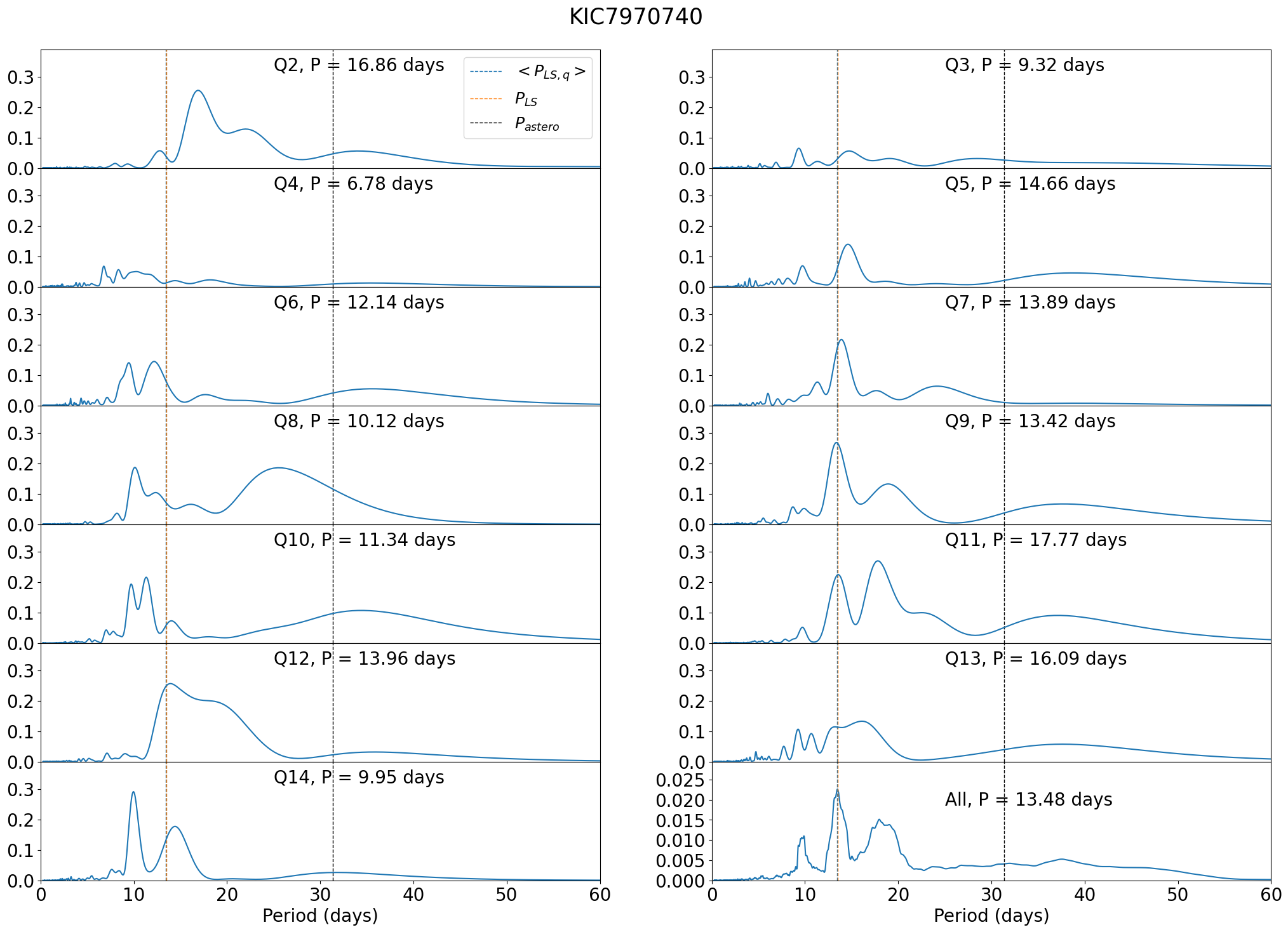
4.3 KOI and non-KOI stars in Group Ab: Kepler-409, KIC 7970740, and KOI-268
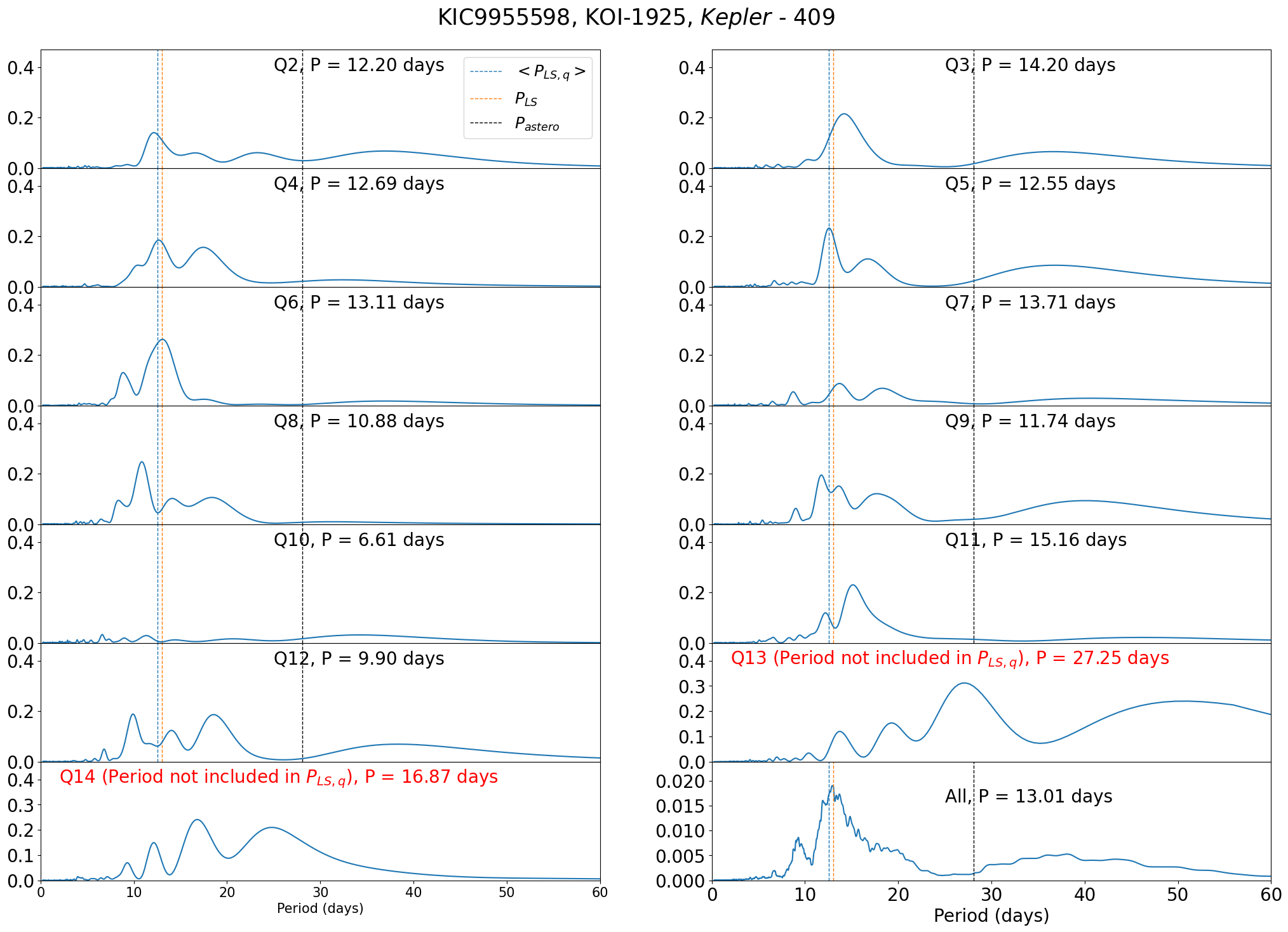
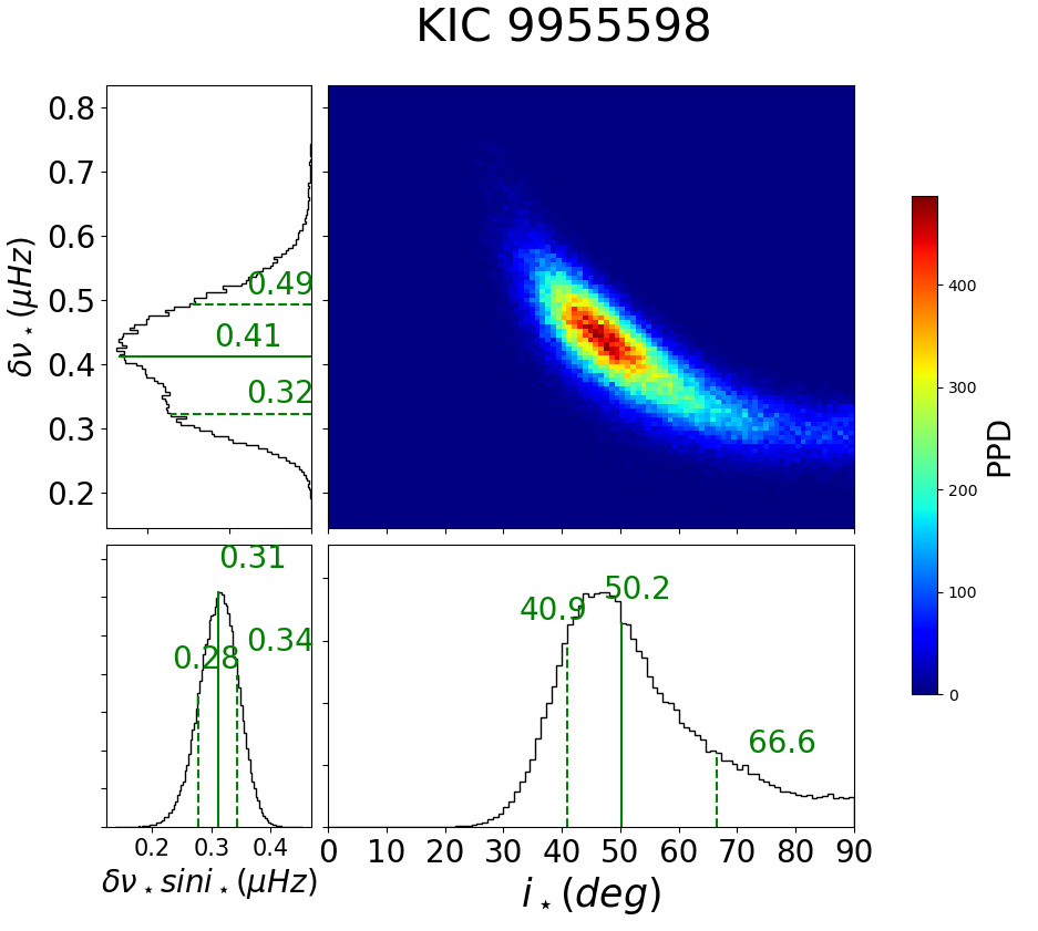
In general, stars classified as Group Ab have consistent estimates for the photometric rotation period as shown in Figure 10. The asteroseismic measurements for group b targets have large uncertainties so that targets do not show statistically significant discrepancy between photometric and asteroseismic periods, except for Kepler-409 (KIC 9955598, KOI-1925) and KIC 7970740.
4.4 KOI stars in Group Ba: Kepler-25, 93, and 128
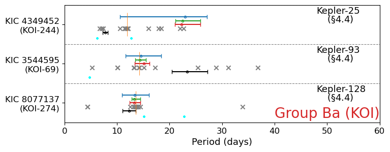
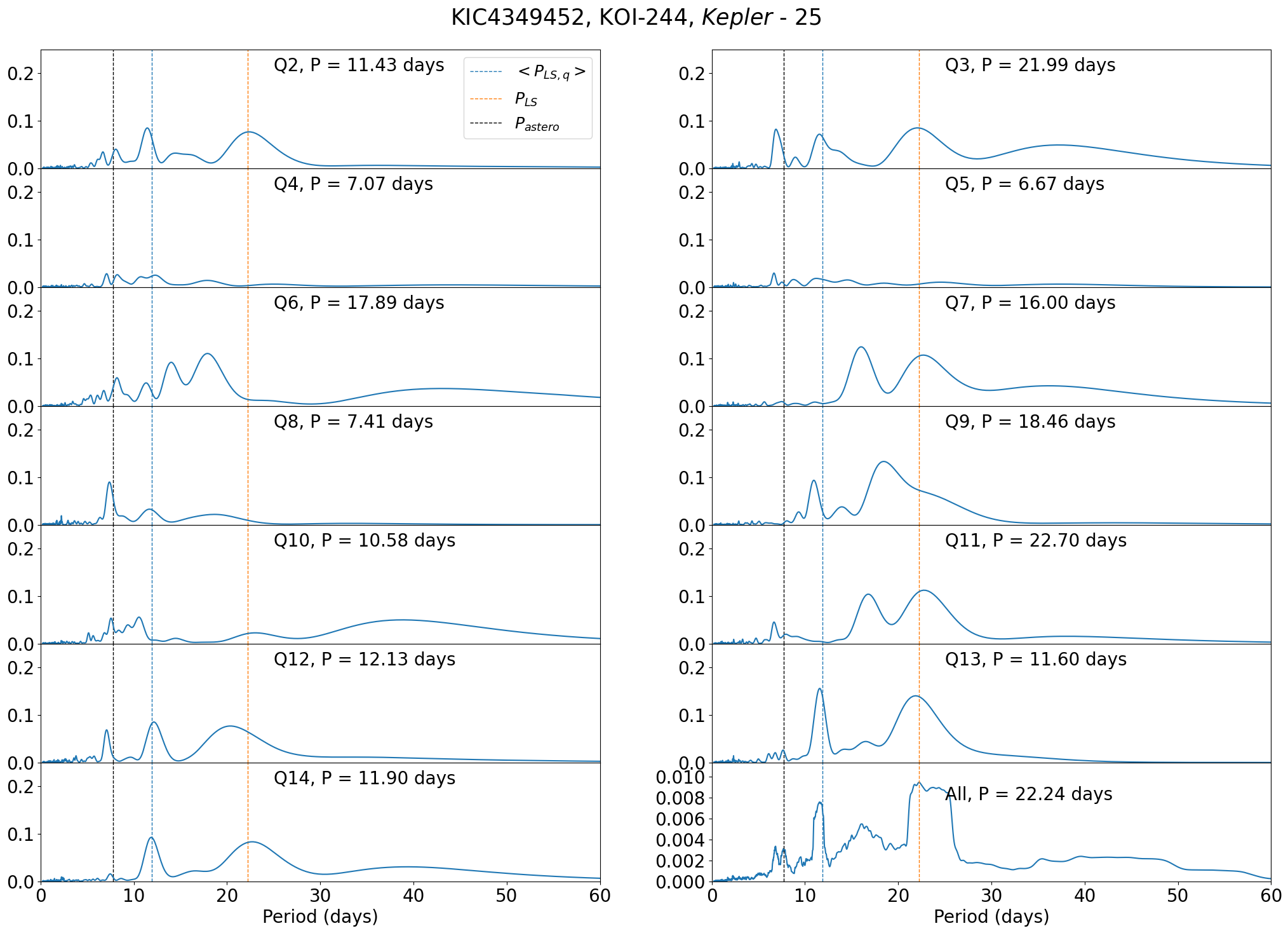
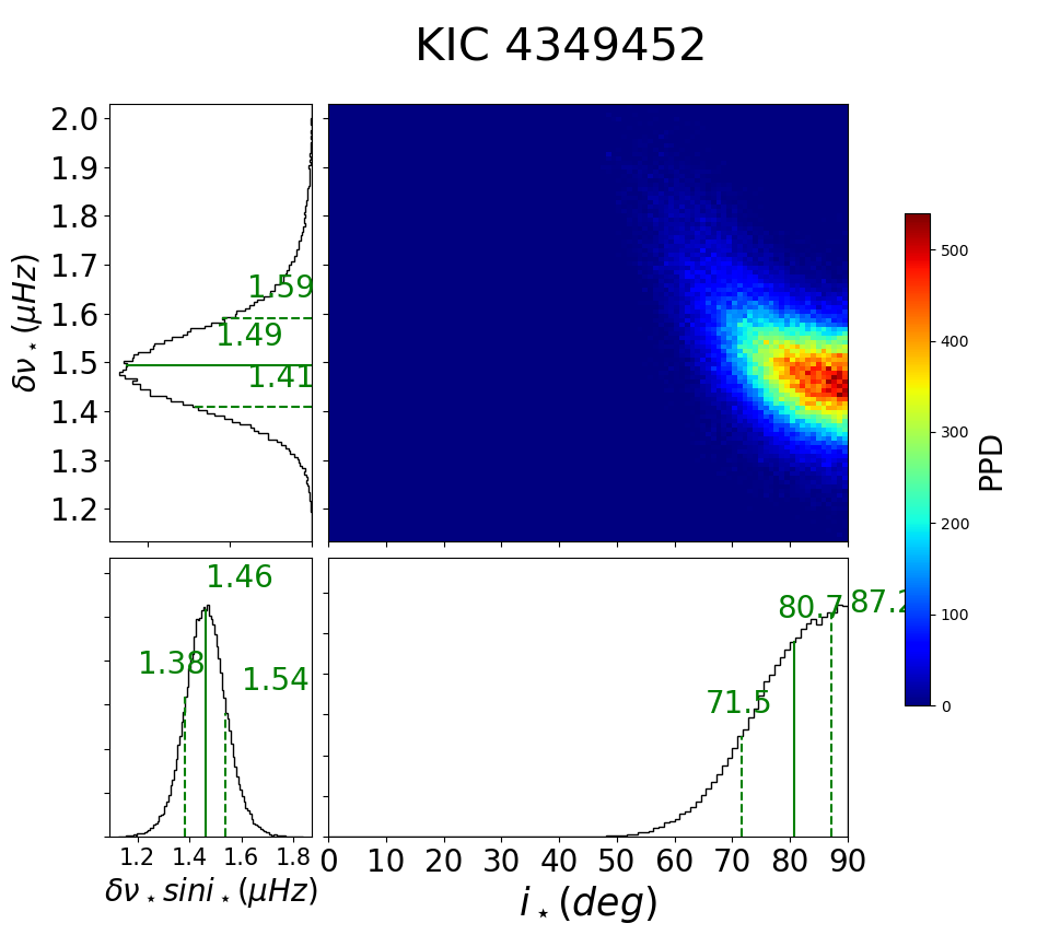
There are three planet-hosting stars in Group Ba (Figure 12). Kepler-25 (KIC 4349452, KOI-244) is one of the two transiting planetary systems for which the real spin-orbit misalignment angle has been estimated jointly from the Rossiter-McLaughlin effect and asteroseismology (Benomar et al., 2014; Campante et al., 2016).
Figure 34 indicates that the photometric rotation period for Kepler-25 varies significantly from quarter to quarter and not reliable. On the other hand, the asteroseismic rotation period seems to be very precisely estimated; days. Adopting km/s and (Marcy et al., 2014), which is in rough agreement with .
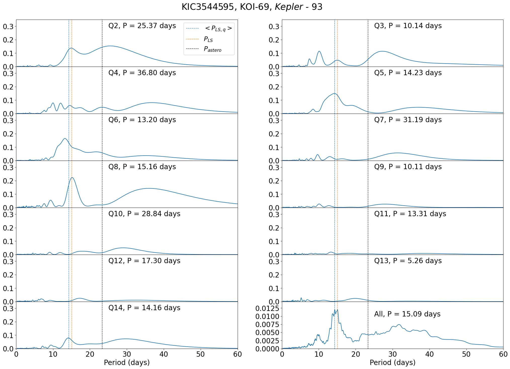
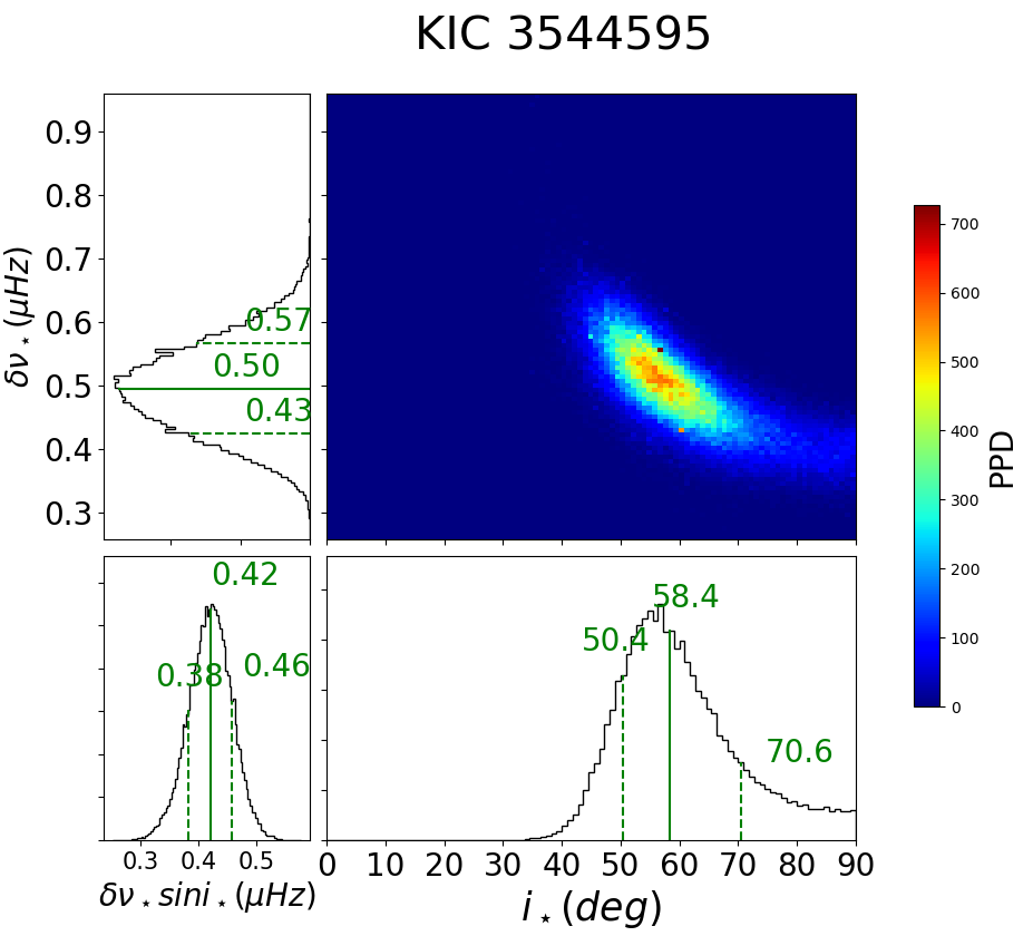
Kepler-93 (KIC 3544595, KOI-69) also exhibits large variation in (Figure 36). Referring to spectroscopic measurement from (Marcy et al., 2014), we obtain days with km/s and . However, such a small value of is not so reliable as it is subject to a large uncertainty in turbulence modeling. On the contrary, asteroseismic analysis provides a relatively precise estimation of days (Figure 37).
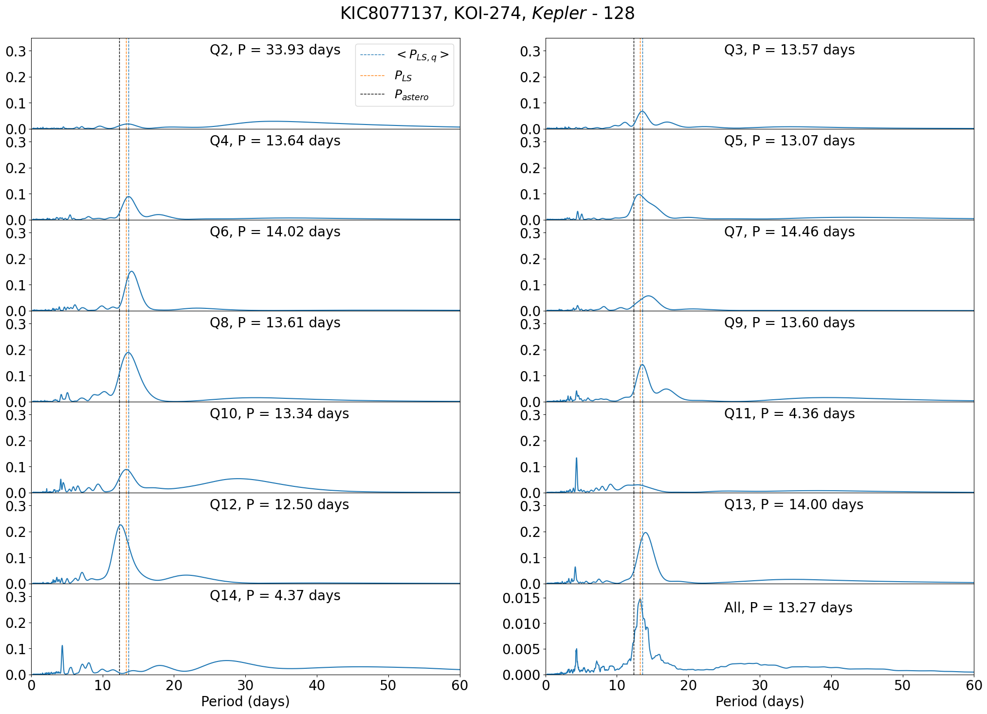
Finally, we note that Kepler-128 (KOI-274, KIC 8077137) is classified as Group B because of three apparent outliers, which are days for Q11 and Q14 and days for Q2. Except for the three quarters, days persistently, and indeed agrees well with days. Thus, Kepler-128 had better be classified as Group A in reality.
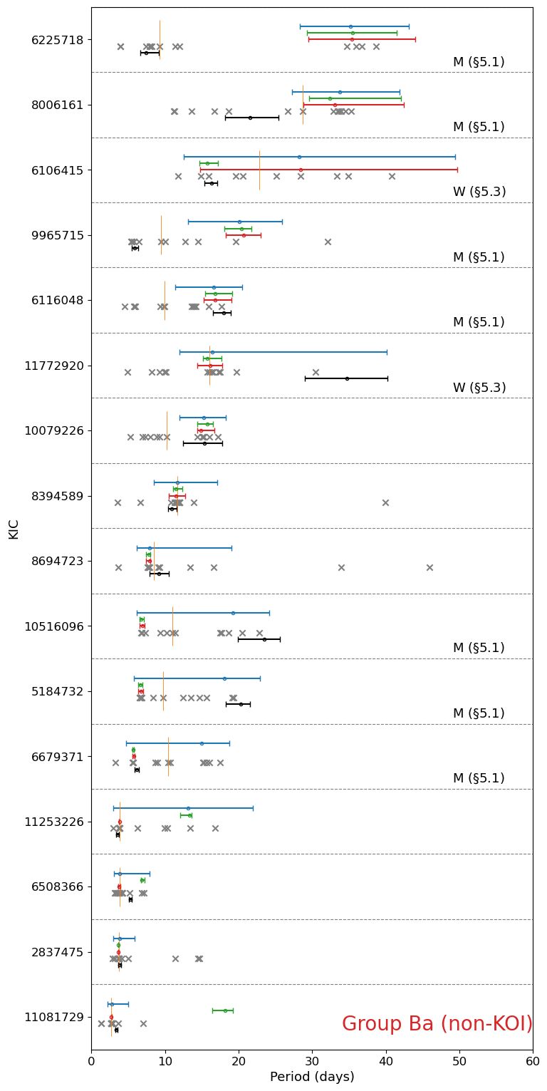
4.5 non-KOI stars in Group Ba
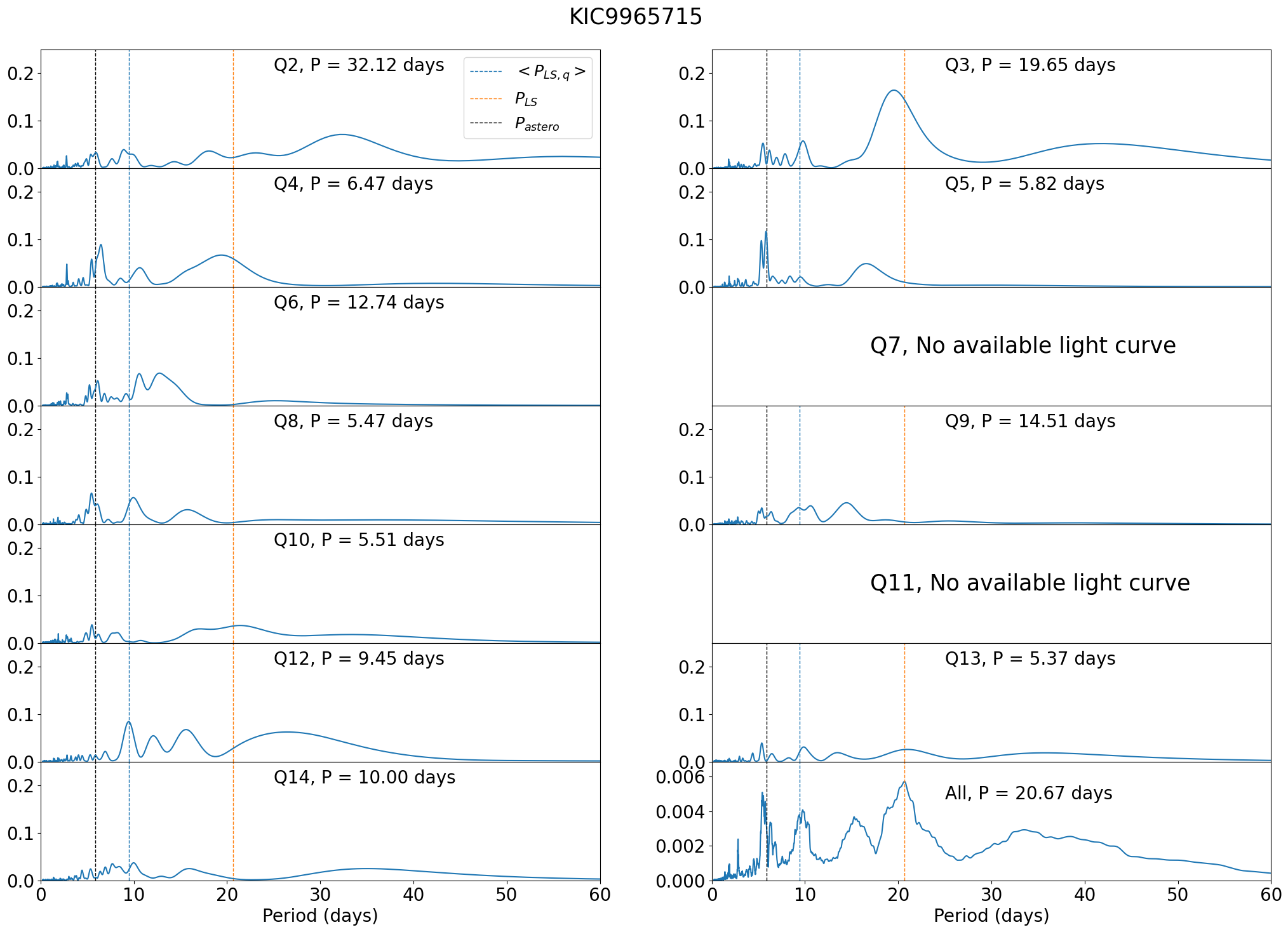
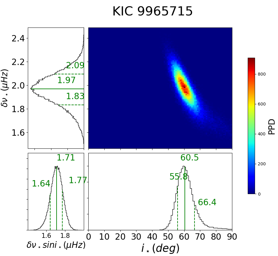
Sixteen non-KOI stars in Group Ba exhibit a diverse distribution of periodicities in the LS periodogram at different quarters. Most of them have multiple peaks whose relative heights vary among different quarters so that it is not easy to determine the photometric rotation period robustly. We show two examples (KIC 6225718 and 9965715) in Figures 46 to 48. As examined in §4.4, is likely to provide better period estimate for stars in Group Ba.
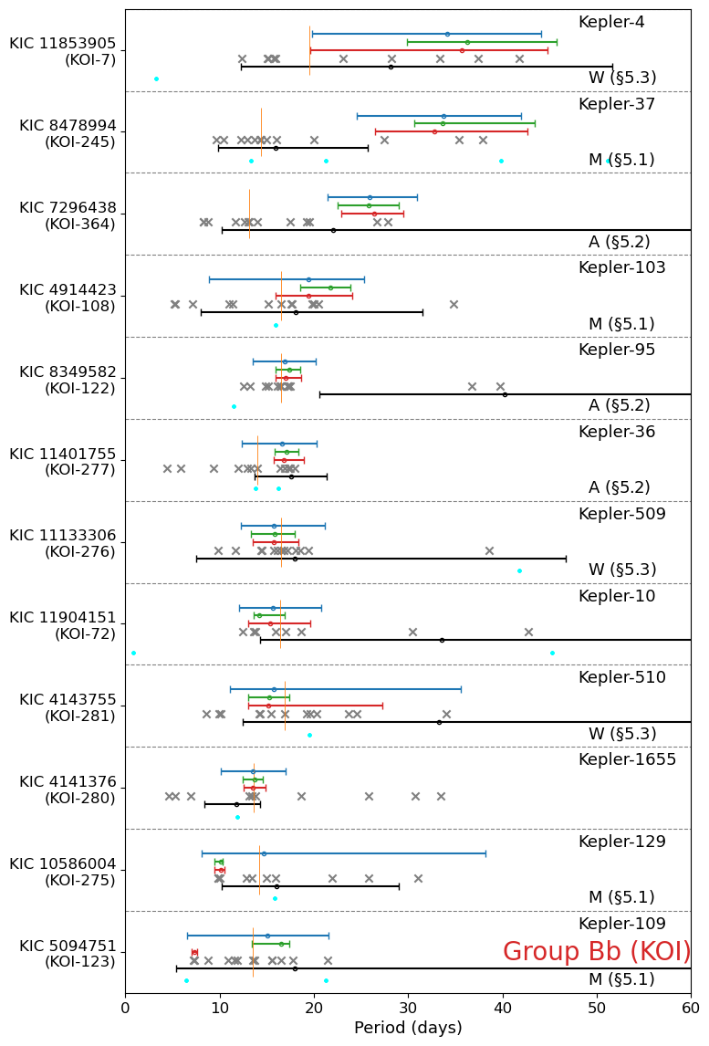
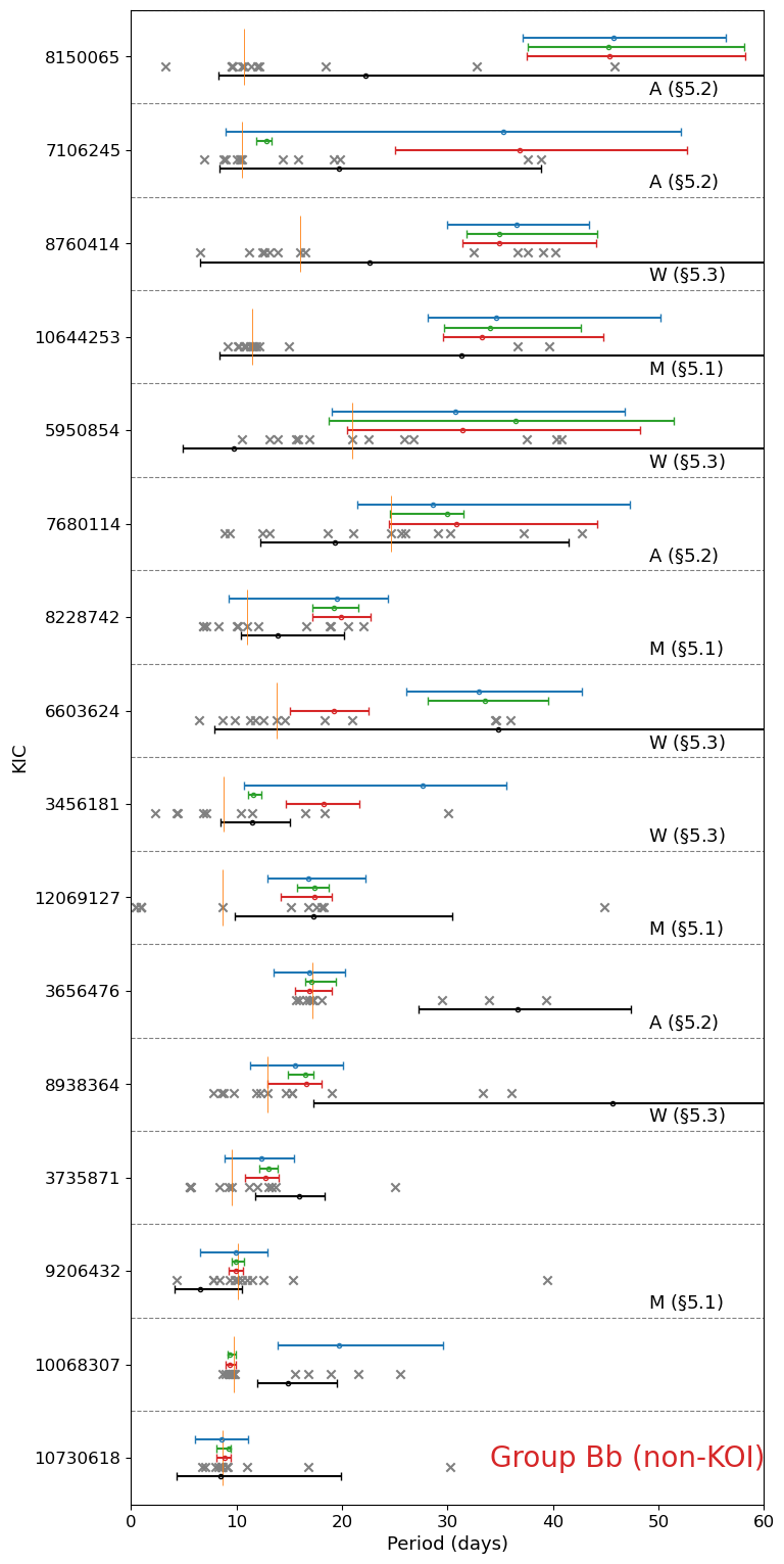
Finally, we show the results for KOI and non-KOI stars in Group Bb (Figures 14 and 15), without discussing them individually.
5 Comparison among photometric analyses
Figure 16 presents the comparison of the rotation periods , , , and . The quoted error-bars for each method are computed according to the description in section A. Thus, they do not necessarily represent the same confidence level, and should be interpreted with caution.
We classified our targets based on defined by equation (1). Thus, the good agreement between and for Group A is as expected; see the lower-right panel of Figure 16. On the other hand, agreement among , , and implies that those photometrically measured periods are reliable and robust, at least for 23 stars in Group A. This should be kept in mind when we discuss the comparison against in subsection 6 below.
The majority of 47 targets in Group B still exhibit consistent rotation periods even though their error-bars are relatively large. Figure 16 shows that 8 stars have inconsistent estimates among , , and ; after careful examination, we find five targets with multiple periodic components, two targets with an anomalous quarter, and one target with no clear periodic signal. We discuss those eight targets individually below.
5.1 Multiple periodic components: KIC 1108172, 11253226, 6508366, 10068307, 5094751
When multiple periodic components exist in the lightcurve, photometric analyses are not enough to discern the true rotation period. In such case, three different analyses assign different relative power to candidate peaks in spectra which occasionally leads to inconsistencies in period detected. For instance, the GWPS is known to increase the power of the fundamental period of a signal (Ceillier et al., 2017), and the ACF method uses a Gaussian smoothing to suppress the short-term modulation including the possible influence of harmonics. Thus both of them may be biased toward a longer period. Here, we provide our interpretation for 5 stars that exhibit multiple periodic components and have different estimates among , , and .
-
•
KIC 11081729 and 11253226: their is much shorter than . The visual inspection of their wavelet power spectra indicates that the short period component persists more than half of the entire observed time span. Thus, is more likely to represent their true rotation periods.
-
•
KIC 6508366 and 10068307: they both have two components roughly different by a factor of two. For KIC 6508366, the shorter period component is observed in the wavelet spectra for all quarters, while the longer period is visible only for a few quarters. For KIC 10068307, in contrast, the two components exist simultaneously within all of the quarters. Thus, we interpret the longer period corresponding to as the true rotation period, while the shorter period being its second harmonics.
-
•
KIC 5094751 (Kepler-109, KOI-123): It has multiple periodic components in Q4 and Q6 with being longer than both and ; see also the right panel of Figure 4. It could be due to a complex spot configuration and/or stellar surface differential rotation, and we can not be certain about which represents the true rotation period.
5.2 Abrupt increase of photometric variation in a single quarter: KIC 3456181, 7106245
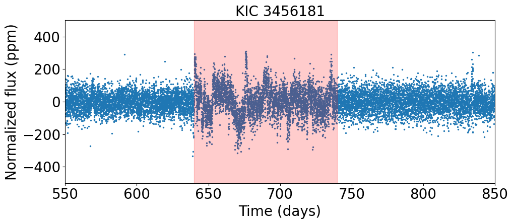
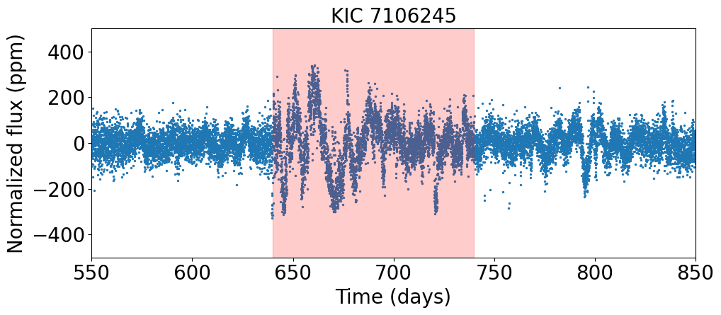
As described in Section 2.2, using a systematic method, we removed anomalous quarters whose median absolute flux variations are three times larger than those of the neighboring quarters for six targets in total; Kepler-1655 (KIC 4141376, KOI-280), Kepler-100 (KIC 6521045), Kepler-409 (KIC 9955598, KOI-1925), KOI-72 (KIC 11904151), KIC 8694723, and KIC 10730618. The goal is to reduce the risk of having a biased measurement. However, among the stars for which the procedure does not detect anomalous quarters (that is, stars for which no quarter removal is performed), there still remains some irregular and abrupt increases in flux, though less prominent, which may affect the estimation of the rotation period.
These abnormal parts might be partly due to residual systematics, or a contamination from other neighbor sources. Such abnormal variation usually give a dominating peak in the power spectrum, over-weighing other weaker peaks that are more likely associated with the actual rotational signals. Examples of this type of light curves are given in Figure 17, whose shaded region shows a strong but transient flux variation. We visual inspect the wavelet spectra of the two given targets and notice that measured low frequency peaks ( 27 days in for KIC 3456181 and 35 days in and for KIC 7106245) are associated with the abnormal regions instead of periodic modulation that we look for. In such circumstance, is less biased by those abnormal quarters.
For all targets in our sample with abrupt increase in flux variation, we check the module and channel number of the abnormal quarters to see whether it comes from a specific CCD plate. However, we notice that such abrupt variations are found in various modules and channels. In addition, we check the position of image on the plate and ensure that the location of image is not around the edge. It is natural to think of the increase in variation as the modulation from a large spot. Nevertheless, known that the lifetime of a spot scales with its size, abrupt variations which last for only 30-40 days seems less likely to be the lifetime of a large spot. Alternatively, such abnormal variation could be the residual of systematics like 30-day re-orientation of telescope. Especially, for relatively ’quiet’ stars with few active regions, there is barely any rotational modulation in the light curve. The residual of systematics would become significant and act like a sudden increase in flux variation.
5.3 Weak or ambiguous periodic variation: KIC 6603624
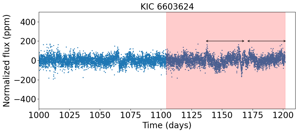
Figure 18 illustrates part of light curves for KIC 6603624 as an example of stars exhibiting a weak flux variation. The WA power spectrum for this type of targets is generally very noisy, and we find that it is simply dominated by the peak at days in Q14 alone for KIC 6603624. As Figure 18 indicated, however, it lasts just for two cycles and it is not clear if it should be interpreted as a rotational feature. Thus, for this type of targets, the measured period is very unreliable, and should be taken with caution. We identify eight such targets with weak or ambiguous periodic components, and label them by “W” in the ’Remark’ column of Table 3, 4, 5, and 6.
6 Comparison between photometric and asteroseismic estimates
Figure 19 compares the rotation period of our targets derived from asteroseismic analysis by Kamiaka et al. (2018) against our four photometric estimates: (upper-left), (upper-right), (lower-left), and (lower-right). Figure 20 plots 17/19 stars whose and do not agree within their uncertainties defined by equations (2), (A7) and (A8). Since we have already discussed most of the 17 targets in §4, we do not repeat such discussion here on an individual basis, but present a few general conclusions below.
First, stars classified as Group Aa are in good agreement except Kepler-100 (§4.1). While it is quite expected from the definition of our classification scheme, it is still encouraging. Second, there exist a population of stars whose is approximately twice of the corresponding photometric estimate. For those stars in Group Ba, is likely to be the true period. For those in Group Ab, on the other hand, it may not necessarily imply that is closer to the true value due to a possible bias toward shorter period for .
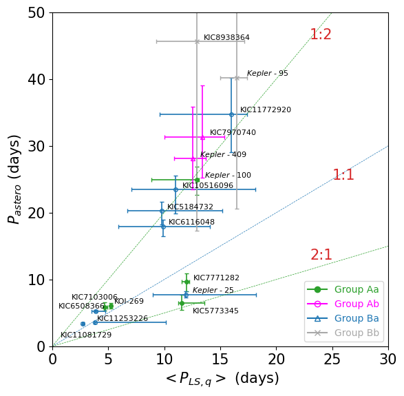
Of course, the difference between and may point to an interesting physical effect, instead of an unknown artifact. Photometric estimates are based on the stellar surface variation, and thus sensitive to the latitudinal and size distribution of starspots, as well as other surface activities, while asteroseismic analysis is supposed to provide an averaged rotation period over a range of latitudes and depths inside the star. On the other hand, Figure 20 seems to suggest a tendency of . This may be interpreted that represents the second harmonics of the true rotation period of , as already pointed out by García et al. (2013). If confirmed, it implies the importance of the complementary visual inspection of automatic photometric analyses.
7 Discussion
7.1 Possible implications for differential rotation
Figures 7 to 15 show that a majority of our targets have a range of different values of in different quarters. The origin of those variations is not easy to identify, and may be a combination of stellar surface activity, instrumental effect, and unknown noise/contamination.
Of course, the variation of could be of physical origin, at least for some targets. The most likely possibility includes an effect of the latitudinal differential rotation coupled with the surface distribution and dynamics of starspots. For instance, the presence of active regions along the same latitude would result in significant peaks with the -th harmonics of the rotation period in the LS periodogram. Such alias would outweigh the fundamental rotation period if such active regions are equally spaced along the same latitude band (e.g. Chowdhury et al., 2018). Furthermore, the co-existence of dark spots (the central darker part, umbra, and surrounding lighter part, penumbra) and brighter spots (faculae) may cancel out part of the photometric variation, which complicates the extraction of the true rotational signal. Our Sun is an example of stars with complex surface configuration (frequent appearance of multiple active regions) which leads to unstable and occasionally low variability in both chromospheric and photometric measurements (see e.g. Donahue et al., 1996; Reinhold et al., 2020). As Donahue et al. (1996) pointed out, it is very likely solar-like star with similar surface configuration to our Sun may not pass the threshold for reliable detection of rotation period.
Consider a simple model of the latitudinal differential rotation (Reiners & Schmitt, 2003; Hirano et al., 2012):
| (5) |
where is the angular velocity of the stellar surface at latitude , is its value at the equator (), and is a parameter characterizing the strength of the differential rotation. For the Sun, .
In order to proceed further, we need to assume the size and latitude distribution functions of starspots and their dynamics (migration over the stellar surface and creation/annihilation timescales), which is unknown. Suto et al. (2022) examined the variation of assuming that the spot distribution in each quarter is independently drawn from the empirical distribution to match the observed flux modulation of the Sun.
For simplicity, we may equate our to the variation of in equation (5). Furthermore, if the spot latitude varies between and , . Thus, in principle, we may estimate individually for our targets. In reality, however, most of the variation of in Figures 7 to 15 are very diverse, implying that the differential rotation combined with the spot distribution may not be dominant except for stars exhibiting modest variations. While we do not conduct further quatitative examination, Kepler-408, KOI-974, Kepler-50, KOI-269, KIC 7103006, KIC 7206837, and KOI-268 may be potentially interesting targets for tightly constraining their differential rotation.
7.2 KOI stars in stellar binary/multiple systems
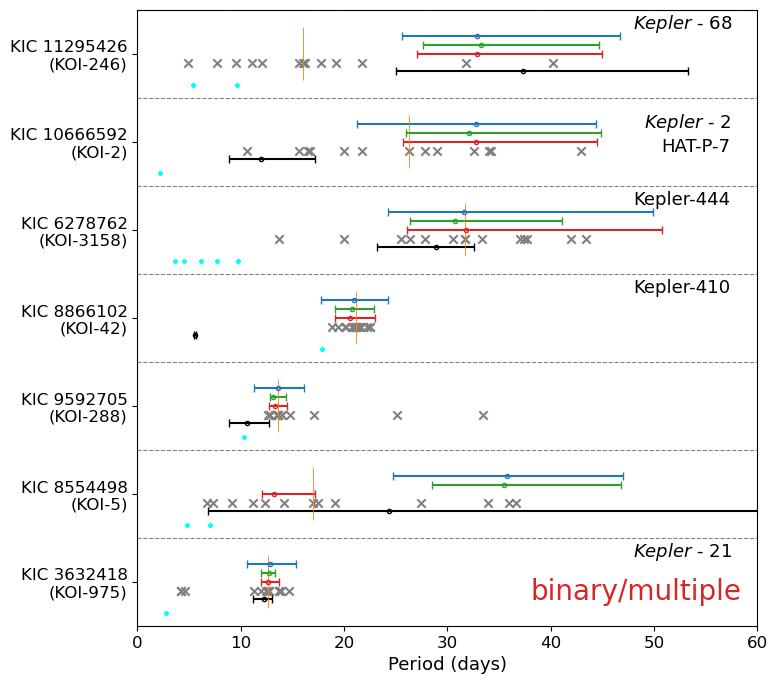
We have 22 stars with possible stellar companions (§2.3). Since their lightcurves might be contaminated by the companions, we exclude them from our main analysis. Nevertheless, we examine seven KOI stars in this subsection because they may have interesting implications for their planetary architecture. Figure 21 plots their rotation periods in the same manner as Figure 7. Among them, we select the following three stars that are potentially interesting, the LS periodogram and asteroseismic constraints of which are shown in §C.11, §C.12, and §C.13.
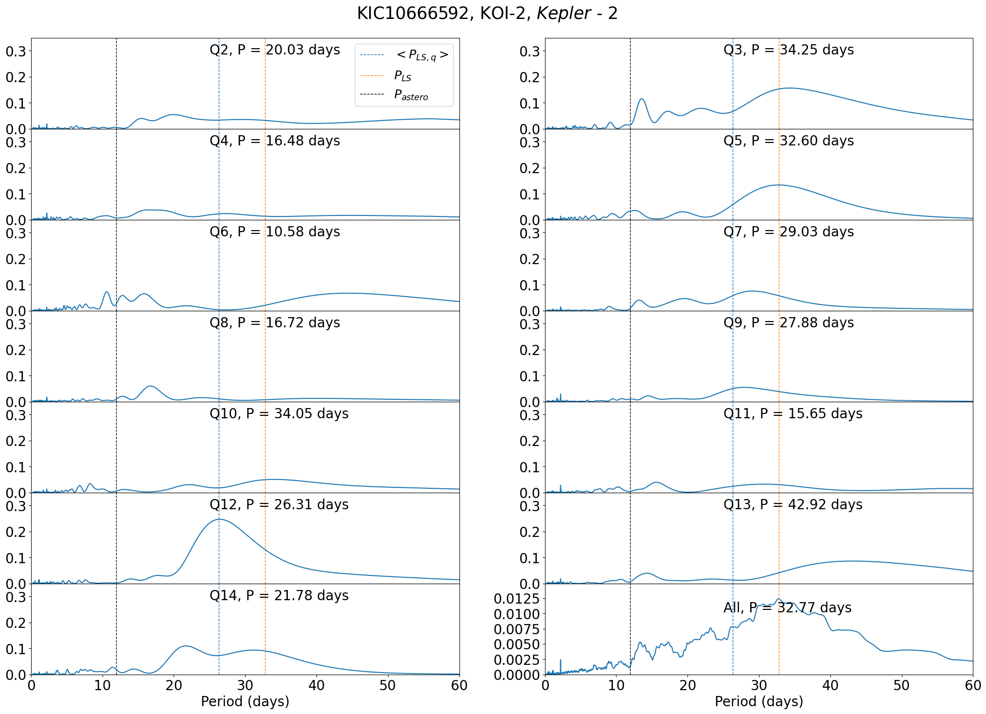
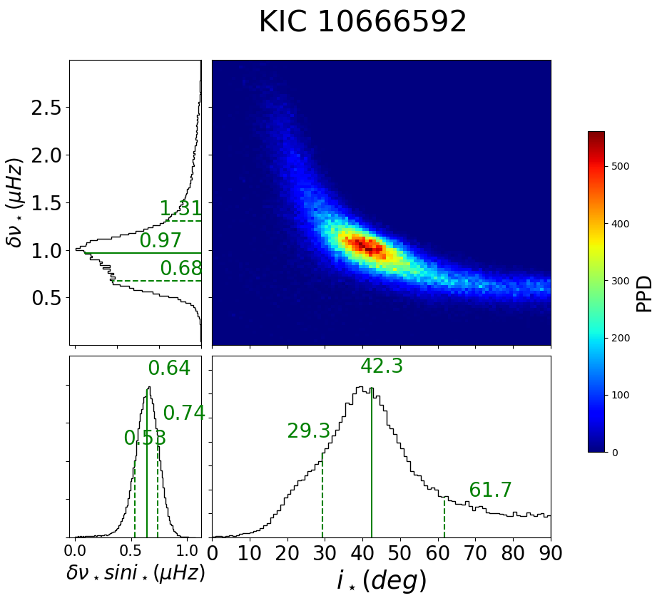
Kepler-2 (HAT-P-7, KOI-2, KIC 10666592) is one of the two transiting planetary systems along with Kepler-25 for which the real spin-orbit misalignment angle has been estimated jointly from the Rossiter-McLaughlin effect and asteroseismology (Benomar et al., 2014; Campante et al., 2016). In reality, however, it is not easy to identify its rotation period photometrically from Figure 50. On the other hand, days from Figure 51 seems to be a reliable estimation of rotation period. This is a good example of the complementary power of asteroseismology.
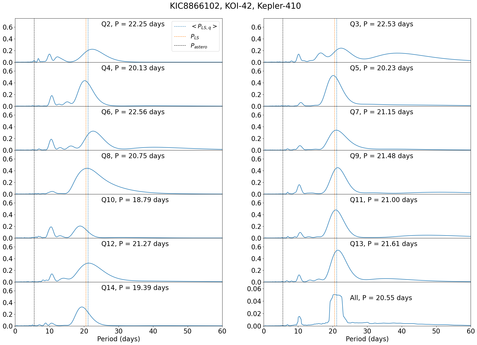
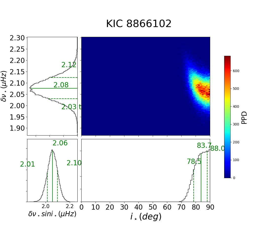
Kepler-410 (KOI-41, KIC 8866102) has precise estimates for both photometric and asteroseismic rotation periods, but their values are very different (). Intriguingly, Figure 52 indicates that the LS periodograms for all quarters have persistent secondary peaks at days, which is very close to the second harmonics of the starspot modulation analytically predicted by Suto et al. (2022). Thus, it is possible that days, instead of 6 days, is the true rotation period of Kepler-410. On the other hand, Kepler-410 is a binary system(Van Eylen et al., 2014), and it is also likely that either asteroseismic or photometric analyses may be contaminated by the companion star to some extent.
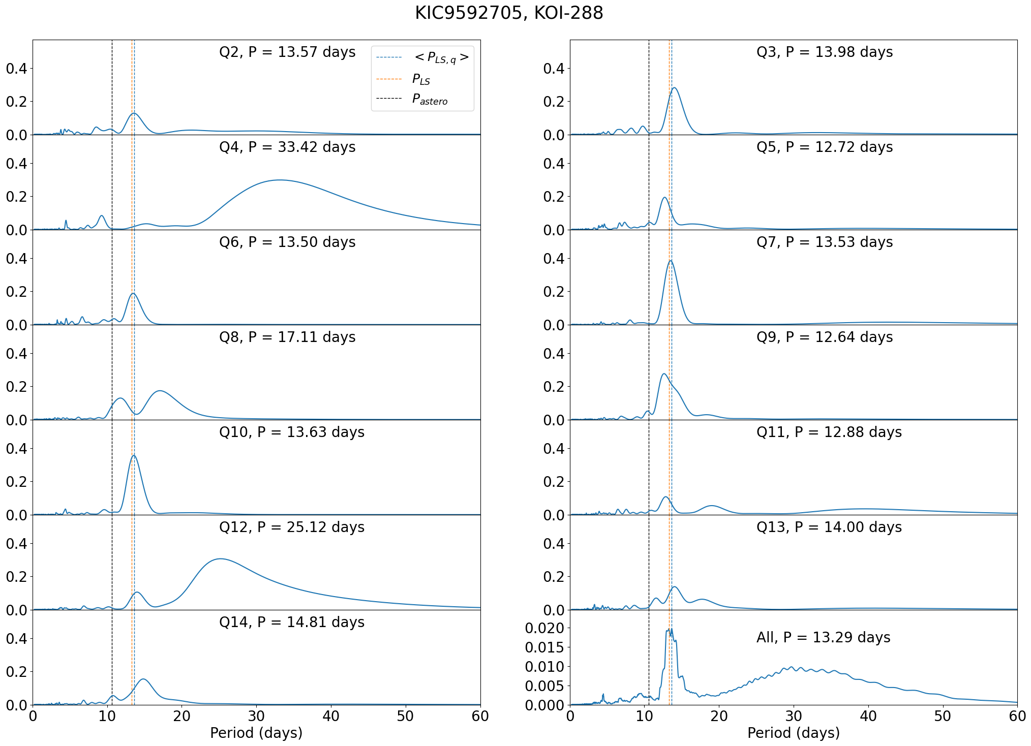
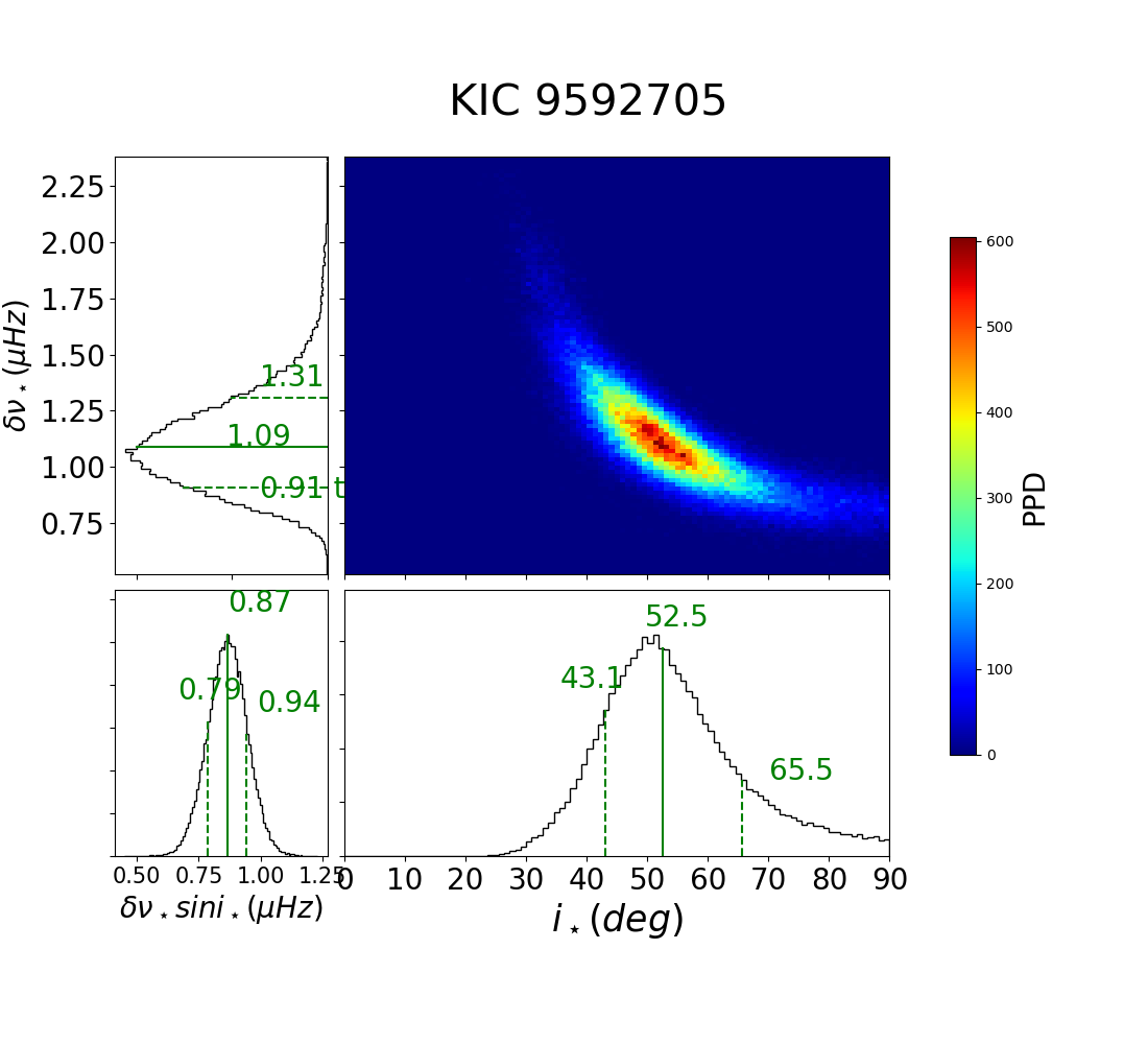
Finally, and of KOI-288 (KIC 9592705) agree within their error-bars. Figure 54 shows that its photometric periods are very robust. Thus, the joint photometric and asteroseismic analysis of KOI-288 may put a tighter constraint on its inclination. Incidentally, this is an example of systems whose is close to the orbital period of the planetary companion (Suto et al., 2019), although it may be just by chance.
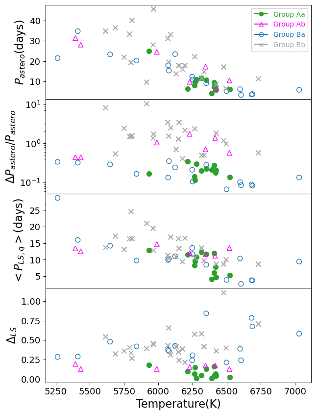
7.3 Photometric and asteroseismic rotation periods as a function of stellar effective temperature
Stars lose the angular momentum through magnetic winds, and the loss rate is supposed to be sensitive to the depth of the convective zone, and therefore to their mass and effective temperature. Indeed, it is known observationally that stars with K have a thicker convective envelope and much slower rotation rate than those with K (Kraft, 1967). Winn et al. (2010) found that hot Jupiters around stars with K prefer the orbital axis well-aligned to the stellar spin axis, and proposed that the spin-orbit alignment results from the stronger tidal interaction between close-in giant planets and their host stars with a thicker convective envelope.
Figure 22 plots the photometric and asteroseismic rotation periods against the stellar effective temperature. We adopt the SDSS from Table 7 of Pinsonneault et al. (2012) for 60 stars. Our result is basically consistent with Figure 3 of Hall et al. (2021) and qualitatively reproduce the Kraft break. On the other hand, our targets with days often have smaller values of and may not properly represent the surface rotation period. Furthermore, the uncertainties of the asteroseismic measurements seem to be anti-correlated with (see Figures 19 and 20).
7.4 Stellar inclinations as a function of stellar effective temperature
Finally, we study the stellar inclination as it could be an indicator of misalignment for planetary systems observed by transit and also has an imprint of the genesis of the stars. The stars are considered as a single population, from which we seek to identify the underlying distribution of stellar inclination and its dependence with temperature. The adopted criteria is the , which is obtained following the method described below.
For the asteroseismic sample of stars, we directly convert the posterior distribution of by Kamiaka et al. (2018), and compute the distribution of . For the spectroscopic determination of , it is required to use equation (3), which depends on , (substituted by the photometric rotation period for the current purpose) and . Furthermore, it is necessary to consider the distribution functions of and and . Here, we assume uncorrelated Gaussian distributions9 for and with their mean being the measured value and standard deviation being its error. Finally, in order to evaluate the distribution of the period, we directly use the LS periodogram of as the underlying probability distribution. However, we only use a range of the LS periodogram that spans over a slice that is twice the HWHM around the highest peak. This distribution is also normalised by integration over the considered range mentioned above. All of the probability distributions of the variables being defined, we then compute the distribution of via Monte Carlo sampling of , and .
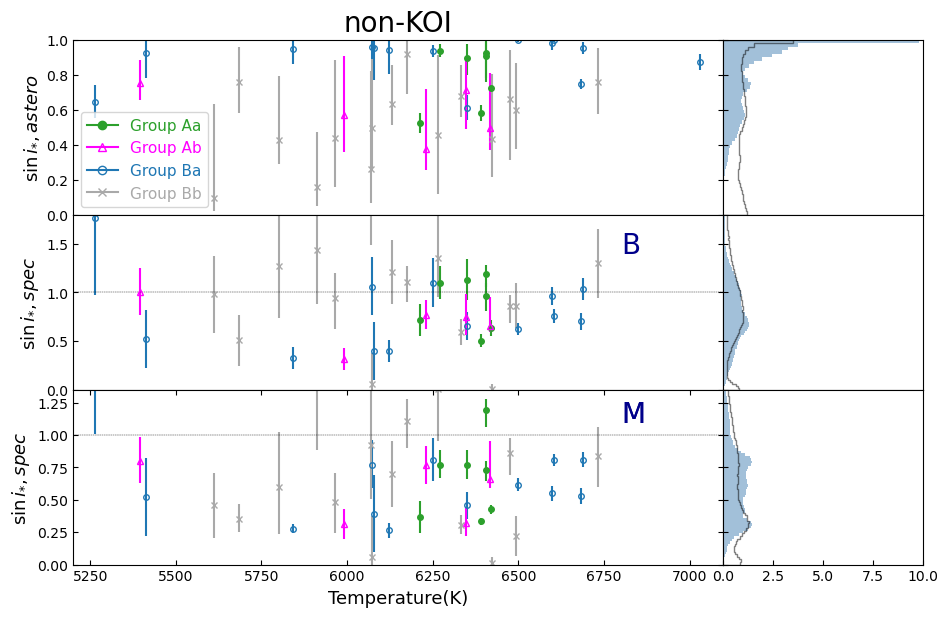
Left panels of Figure 24 plot and for KOI stars against the stellar effective temperature following the same procedure as described in Kamiaka et al. (2018) (in their Section 5.3), while right panels show the corresponding distribution functions.
Although the sample of KOI stars is small, we note that if one excludes stars from Group Bb (the least reliable stars), KOIs tend to have clustered around unity, and that spectroscopy and seismology are in good agreement. This indicates that a majority of stars with planets show a preference for a spin-orbit alignment, which is consistent with the previous conclusion by Kamiaka et al. (2018).
Figure 24 focuses on non-KOI stars. Excluding stars from Group Bb, exhibits a broader distribution compared to KOI stars. We note that the distribution is not uniform in as it would be expected if there was no preference in their rotational spin direction on the sky. As shown by Kamiaka et al. (2018), asteroseismology overestimates inclinations below , corresponding to . This is likely the cause for a lack of population with reliable measurement when . In addition, as pointed out by Kamiaka et al. (2018), available spectroscopic measurements are unreliable for some stars, in particular when the is low (due to the dominance of the stellar turbulence). Therefore, spectroscopic results from Molenda-Żakowicz et al. (2013) and from Bruntt et al. (2012) sometimes lead to a mathematically inconsistent result of . If we exclude these impossible cases, there is no clear preferential stellar inclination. This is again consistent with an isotropic distribution of stars and contrasts with results from the KOI case shown in Figure 24.
7.5 Complementarity of photometric and asteroseismic analyses
This paper has performed comprehensive photometric analyses of the 92 Kepler stars selected by Kamiaka et al. (2018) for the asterosesmic analysis. The photometric intensity variability measures the period of rotational modulation caused by the active regions at a specific latitude on stellar surface. The asteroseismic analysis, on the other hand, studies the pulsation pattern and derives an averaged rotation period over a range of latitudes and depths inside the star. Since stars are not ideal solid-body rotators, their radial and latitudinal differential rotations would affect the estimates of their rotation periods in different methods. Therefore, the comparison between the photometric and asteroseismic results provides unique and complementary insights into the nature of those targets. One of the most important examples is the stellar inclination angle measured from asteroseismic analysis, which is a key ingredient for measuring a three-dimensional spin-orbit angle of exoplanetary systems (see e.g. Benomar et al., 2014; Winn & Fabrycky, 2015; Kamiaka et al., 2018, 2019; Suto et al., 2019). While the asteroseismic analysis provides a unique relation between the stellar inclination and the rotation period, its degeneracy is not easy to be broken by asteroseismology alone (see Kamiaka et al., 2018). When a more precise estimate of the rotational period is available from the intensity variability, it is very useful to break the degeneracy. Hence, a detailed examination of various photometric methods as presented in this work provides an important framework for those complementary approaches.
8 Summary and conclusions
We have performed a comprehensive photometric and asteroseismic analysis of 92 solar-like main-sequence stars observed by Kepler. We focus on 70 stars that do not have stellar companions, and classify them in four groups (Aa, Ab, Ba, and Bb) according to the fractional variance and precision of the rotation periods and ; see §3.1 and 3.2. We have presented detailed comparison among photometric and asteroseismic constraints for those stars on an individual basis.
Group Aa has 14 stars with robust estimates for both and . Twelve out of the 14 stars have as expected. The remaining two include Kepler-100 ( days and days), and KIC 5773345 ( days and days); see §C.1 and C.2. They are potentially interesting targets for further study. Group Ab has 9 stars. For these stars, is consistent with , except for Kepler-409 and KIC 7970740; see §C.6 andC.7.
There are 19 stars in Group Ba and 28 stars in Group Bb. Since their photometric rotation periods vary from quarters to quarters, it is not easy to assign definite rotation periods photometrically. For stars in Group Ba, provides a better estimate for the true rotation period without being affected by the stellar surface activity. It is interesting to note that the stars for which photometric and asteroseismic periods are different exhibit a tendency of (Figure 20). This may imply that represents the second harmonics of the true rotation period of , at least for some of those stars.
We find that there are 4 KOI stars in our sample whose rotation period agrees with the orbital period of their planetary companion; Kepler-65 (Group Aa), Kepler-50 (Group Aa), Kepler-1655 (Group Bb), and KOI-288. Due to a limited number of our sample, this may be simply a statistical fluke and not definitive, but could imply a possible interaction between the star and planet in those systems (Suto et al., 2019).
Most of stars exhibit significant quarter-to-quarter variations of , which come from the combined effects of the differential rotation, various stellar surface activities, and other noises. Among them, 7 targets including Kepler-408, KOI-974, Kepler-50, KOI-269, KIC 7103006, KIC 7206837, and KOI-268 may be potentially interesting in constraining their differential rotation.
Our main findings are summarized as follows.
-
1.
Most of our targets exhibit significant quarter-to-quarter variances in the photometric periods. This is reasonable, given the complicated dynamics and activities of the stellar surface and starspots. Thus, the estimated photometric period should be regarded as a simplified characterization of the true stellar rotation period, especially under the presence of the latitudinal differential rotation.
-
2.
There is a fraction of stars with a relatively small quarter-to-quarter variance in the photometric periods (Group A; 23 out of 70 stars in our sample), for which the three photometric methods (the Lomb-Scargle periodogram, autocorrelation function, and wavelet analysis) enable the precise determination of the stellar rotation period in a consistent manner. Furthermore, it is encouraging that the asteroseismic rotation period for most of those stars agrees with the photometric rotation period within their uncertainties. Thus, rotation periods for stars satisfying our photometric classification condition should be reliable and accurate even without the asteroseismic estimate (that is not available in most cases).
-
3.
Rotation periods more than 30 days either photometrically or asteroseismically are not reliable in our Kepler sample. They may suffer from some residual systematics or correspond to the harmonics, and should be interpreted with caution. If the 30-day systematic trend is caused by the monthly re-pointing of Kepler, it will vanish in other missions with less frequent re-orientation such as PLATO (Rauer et al., 2014).
-
4.
There are 19 stars whose photometric and asteroseismic periods are not consistent. They should be potentially interesting targets deserved for further individual investigations.
We would like to note that the large variability observed in some stars and reflected by our classification might be further explored in another study. Indeed, in some stars and through a spot modeling, it may be possible to estimate the latitudes of the spots, their migration over time and the stellar rotation profile.
Appendix A Methods to estimate the stellar rotation period
There are a variety of methods to identify the periodicity in the photometric variations of the light curve. Among them, the Lomb-Scargle (LS) periodogram, autocorrelation function (ACF), and wavelet analysis (WA) have been applied extensively to the high-quality photometric data from space missions including Kepler.
For instance, Nielsen et al. (2013) applied the LS periodogram to Kepler main-sequence stars and detected their rotation periods. McQuillan et al. (2014) measured rotation periods of Kepler main-sequence stars using autocorrelation function. García et al. (2014) estimated the rotation period of 310 solar-like stars by combining autocorrelation function and wavelet analysis. Finally, we consider the asteroseismic rotation periods obtained by Kamiaka et al. (2018).
Even though those methods have been widely used in the literature, they may have their own advantage and disadvantage. Thus, we compute the rotation periods separately derived from the four methods. The detailed comparison of the resulting values is useful in understanding their robustness and reliability. In what follows, we briefly describe the basic principle of the four methods, together with typical examples of their outputs.
A.1 Photometric analysis
A.1.1 The Lomb-Scargle periodogram
The LS periodogram is one of the most popular methods to detect periodic signals embedded in the data (Lomb, 1976; Scargle, 1982). Specifically, we adopt the generalized LS periodogram by Zechmeister & Kürster (2009), which fits the data to a single -mode sinusoidal function of frequency and a constant term. We denote the resulting best-fit squared residuals at each frequency as . In the present paper, we adopt the standard normalization:
| (A1) |
where is the best-fit squared residuals with respect to a non-varying constant reference model.
We compute equation (A1) for each target at frequencies:
| (A2) |
where is an integer, and we set and so as to cover the range of the rotation period of the solar-type stars. The frequency interval is set to be , where is the total time span of the light curve for each star (typically days), the oversampling factor is chosen to be (see VanderPlas, 2018, e.g.,).
Finally, we smooth the periodogram sampled at using a box-car filtering over 0.1 Hz to suppress the spurious discreteness effect in the frequency space.
Figure 25 shows an example of the LS periodogram in time domain, i.e., . We identify the highest peak in the smoothed periodogram, and estimate the LS rotation period and the associated errors and from the peak location and the corresponding HWHM (half width at half maximum) as illustrated in the vertical line and boundaries in the blue shaded region of Figure 25.
We repeat the same procedure using the light curve for the -th quarter (each with days) separately, and obtain (). As we discuss extensively below, the distribution of for different and the comparison against are useful in examining both the reliability of the measurements and the degree of the latitudinal differential rotation due to the non-static nature of starspots.
We note here a fairly common problem in selecting the the highest peak in the LS periodogram as the stellar rotation period . Figure 25, for example, shows another significant peak around 4 days, and it could correspond to a true rotation period, a higher harmonic, or a false positive due to stellar surface activity, instrumental noise, and/or contamination from possible companions (e.g. Reinhold & Reiners, 2013; Santos et al., 2017; Chowdhury et al., 2018). It could also come from the symmetric distribution of starspots (Suto et al., 2022). Hence, we examine the reliability of the highest peak in the LS periodogram by repeating the analysis in individual quarters and also through the close comparison against other complementary methods, in particular a time-localized spectrum-wavelet power spectrum.
A.1.2 Autocorrelation function
We compute auto-correlation function (see e.g. McQuillan et al., 2013, 2014) of the light curve :
| (A3) |
Then, we smooth using the Gaussian filter of in order to suppress the short-term modulations unrelated to, and/or the harmonics of, the stellar rotation.
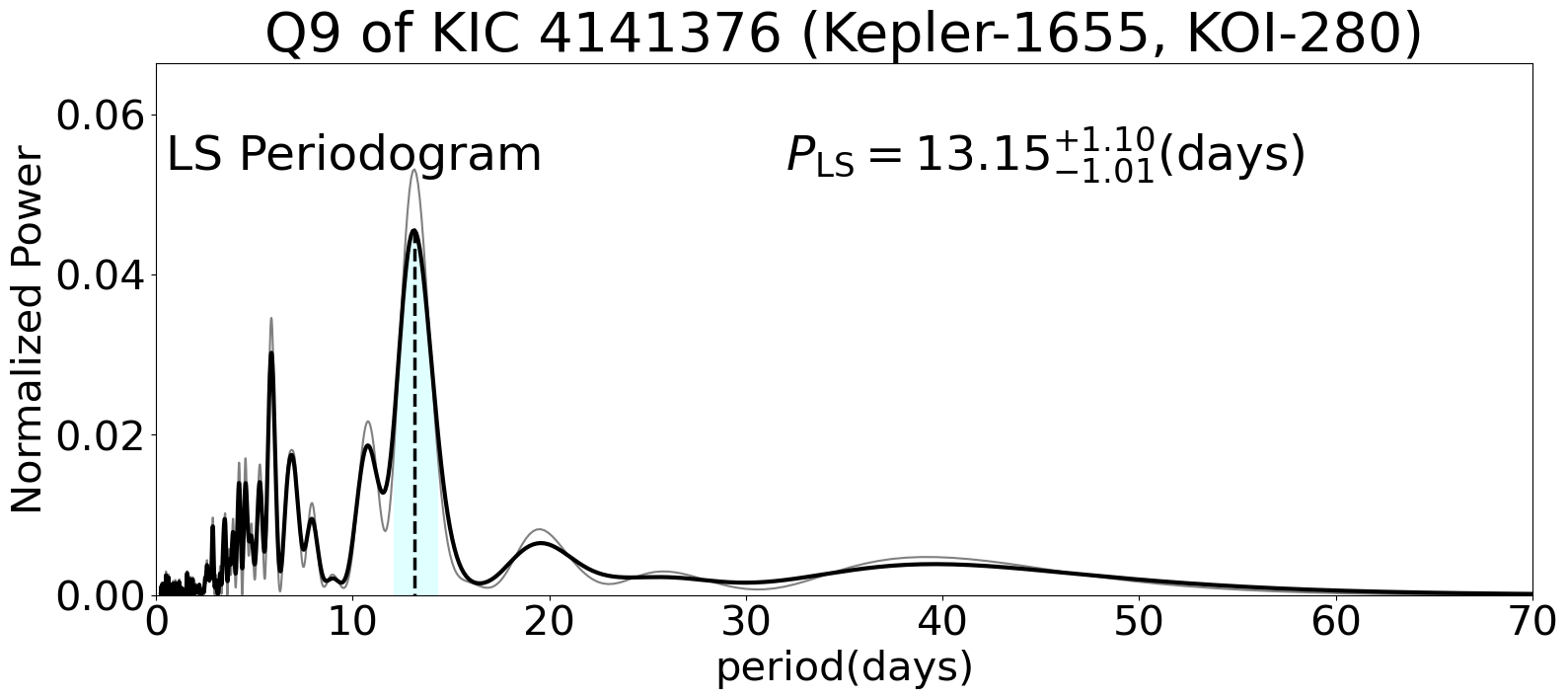
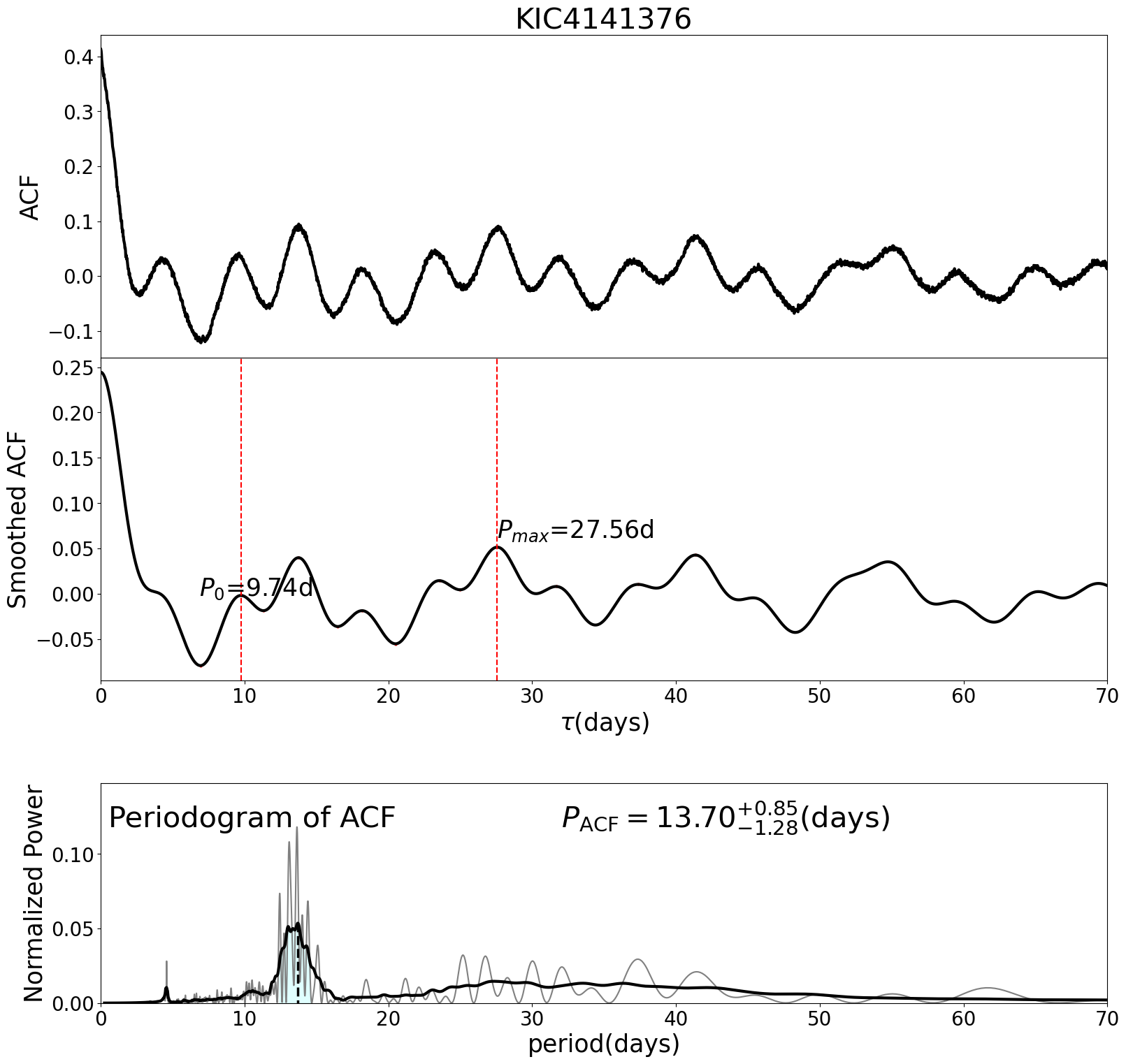
Figure 26 shows examples of the ACF analysis for Kepler-1655 (KIC 4141376, KOI-280). The periodic patterns in the top and middle panels are the clear signature of the stellar rotation. A substantial fraction of our current targets, however, exhibits a more complicated pattern. So we apply the generalized LS periodogram to the smoothed ACF, and extract the embedded period. Following the procedure described in §A.1.1, we define the stellar rotation period and the associated uncertainties from the ACF method.
A.1.3 Wavelet
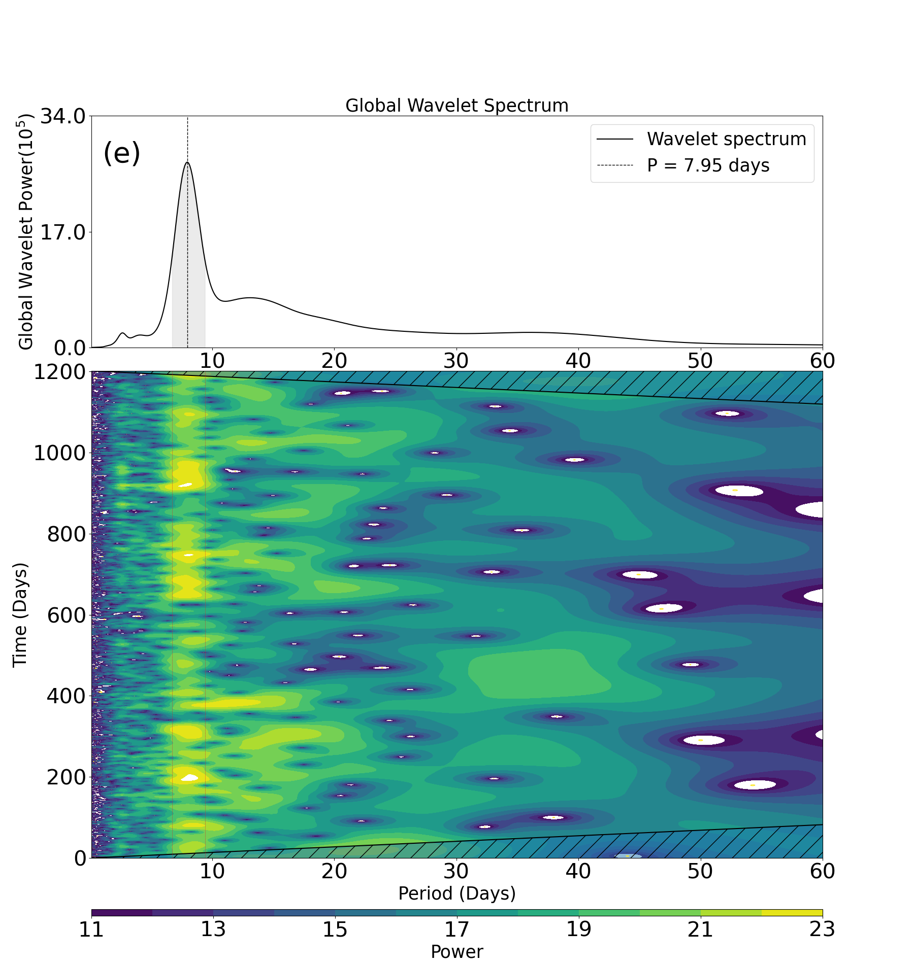
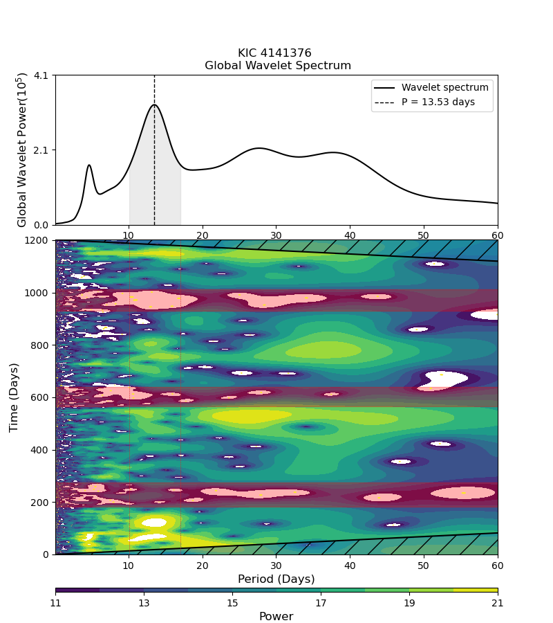
Wavelet analysis (WA) is one of the widely applied methods that identify time-dependent signals in a time-frequency domain. Since the photometric variations in the stellar light curves are time-dependent over the observed duration () reflecting the dynamical nature of spots on the stellar surface, WA is naturally suited for the detection of the underlying stellar rotation period including the possible effect of the differential rotation.
Following Torrence & Compo (1998); García et al. (2014), we adopt the Morlet wavelet that corresponds to a sinusoidal wave localized in the time domain using a Gaussian window of the form:
| (A4) |
and search for the best-fit value of the scale . The dimensionless parameter in introduced to control the resolution in the time-domain, and we adopt the common value of . The scale is related to the period of the signal in the standard Fourier mode as
| (A5) |
Torrence & Compo (1998). In practice, we search for in the range between 0.1 days and 65 days in a linearly equal bin of 0.1 days.
Figure 27 presents an example of WA for Kepler-1655 (KIC 4141376, KOI-280). The left panel shows the wavelet power spectrum (WPS), while the right panel is the corresponding global wavelet power spectrum (GWPS). GWPS is defined as the average of WPS over time axis multiplied by the variance of the time series. Note that the wavelet spectra in the present paper are plotted against , equation (A5), instead of . Finally, we define the WA rotation period from the highest peak in the GWPS, and compute the uncertainties based on its HWHM.
While the above definition of the uncertainties in GWPS turns out to be generally larger than those in LS and ACF, this may be simply due to a matter of definition, given the fact that a majority of their peak profiles is far from Gaussian nor symmetric. Thus, their quantitative interpretation and comparison against other results should be made with caution.
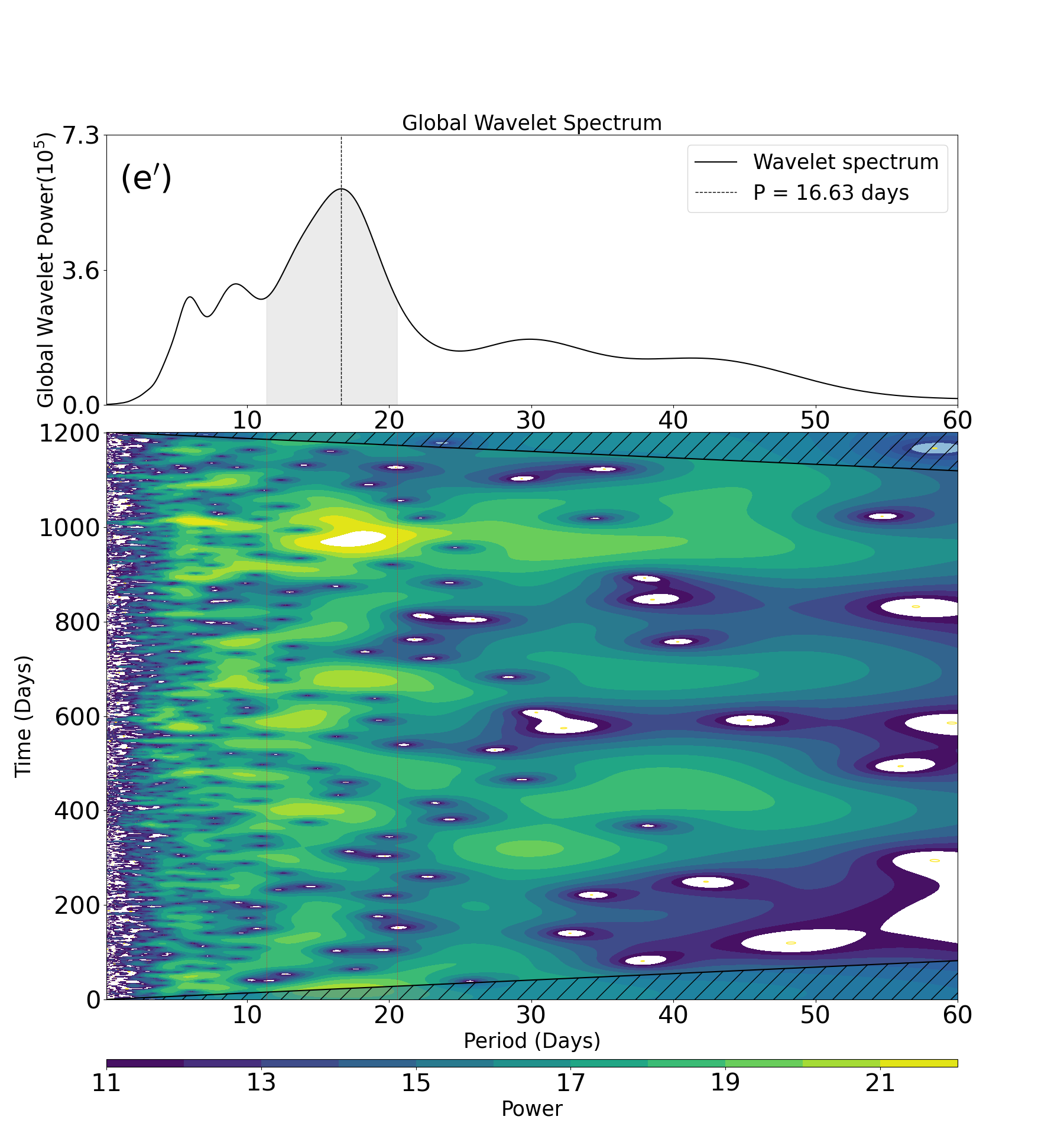
Instead, we would like to emphasize that WPS provides useful information on the time-dependence of the measured stellar rotation period over the entire observing time, which is likely related to the strength of the differential rotation of each star. This is the most important and complementary aspect of WA. For instance, the left panel of Figure 27 indicates that the measured rotation period is relatively stable and does not show any detectable variation, implying that the differential rotation is very weak and/or that those spots responsible for the photometric variations are static over a timescale of 1200 days.
It is also important to note that Figure 27 clearly indicates that the peak around 4 days exhibited in Figures 25 and 26 mainly come from the contribution of Q2. While it is not clear why Q2 behaves very differently from the other quarters, WA strongly indicates that the 4 day period does not correspond to the true stellar rotation period. This illustrates the complementary role of the WA relative to other methods.
A.2 Asteroseismic analysis
Asteroseismic analysis estimates the stellar rotation frequency and inclination by modeling the pulsation pattern of stars around a few thousands Hz (see Ledoux, 1951; Tassoul, 1980; Gizon & Solanki, 2003; Mosser et al., 2013, e.g.,).
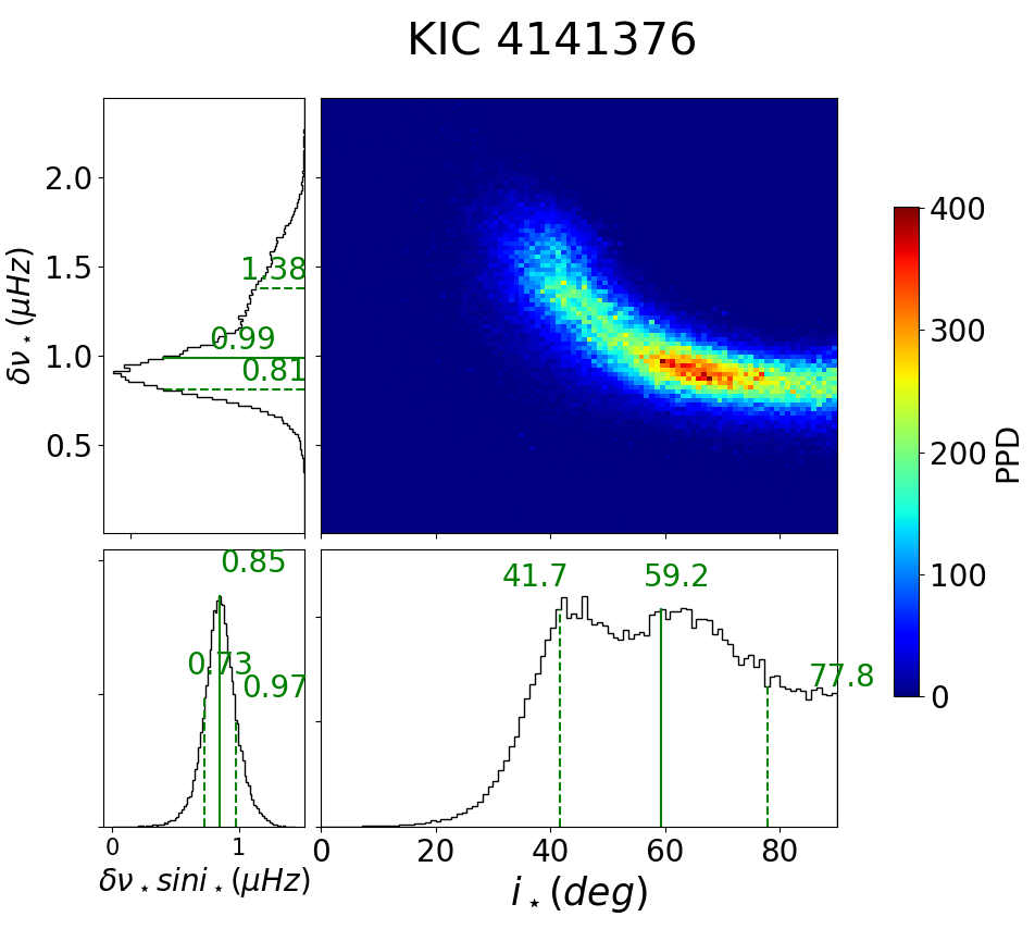
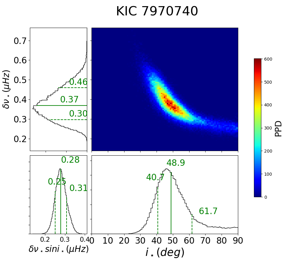
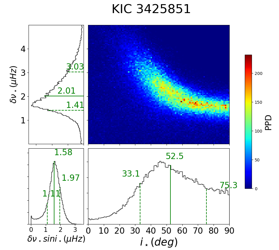
Figure 28 shows an example of constraints on and for Kepler-1655 (KIC 4141376, KOI-280), derived from asteroseismic analysis by Kamiaka et al. (2018). Following them, we define the asteroseismic rotation period and their uncertainty as
| (A6) | |||||
| (A7) | |||||
| (A8) |
where refers to the value at the percentile in its one-dimensional marginalized density (top-left panel in Figure 28). We emphasize that the above definitions are not necessarily unique, and that the comparison against the photometric rotation period needs to be interpreted with caution especially when is large. We adopt the asteroseismic result by Kamiaka et al. (2018) for all the target stars. Further details of their analysis may be found in Kamiaka et al. (2018), Kamiaka et al. (2019), and Suto et al. (2019).
Appendix B Comparison with previous photometric analysis
Among our 70 targets discussed in the previous section, 44 have their photometric rotation periods published in previous literature. Left panel of Figure 29 plots the comparison of the rotation periods derived from the same photometric method. We use different colors to distinguish the four groups that we introduced in the previous section, while different symbols indicate different papers shown in the caption; from Nielsen et al. (2013) and Karoff et al. (2013), from McQuillan et al. (2013) and McQuillan et al. (2014), and from Ceillier et al. (2016) and García et al. (2014). Right panel of Figure 29 plots the rotation periods in previous literature against our on which our photometric classification is based. In what follows, we present detailed discussion of the comparison against those papers individually.
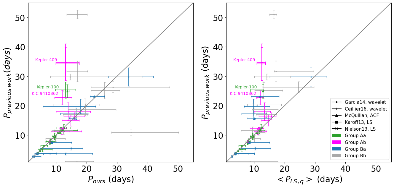
B.1 Nielsen et al. (2013)
Nielsen et al. (2013) first conducted the LS analysis for Q2 to Q9 separately, using the Kepler PDC-SAP light curve (SAP is light curve without removal of systematic effect. msMAP is light curve which has been processed, e.g. removal of systematic effect). They assume that should be within days and define the median of those as as the rotation period, . Among their final sample of 12151 stars, we have 7 targets in common; 5 targets belong to our category of likely binary/multiple-star systems (see Table 2) which we exclude in the comparison, and the other two stars (KIC 7206837 and 9812850) belong to our Group Aa and their rotation periods are in good agreement with our .
B.2 Karoff et al. (2013)
Similarly, Karoff et al. (2013) performed a quarter-wise LS analysis for a sample of 20 stars using Q2-Q14 of Kepler PDC-SAP. They defined from the peak with S/N higher than 4 in all 14 quarters. We have 8 overlapped targets, 4 in the category of likely binary/multiple-star systems. The remaining 4 targets in Group Aa (KIC 12009504) and Group Ba (KIC 2837475, KIC 11253226, KIC 8694723) have rotation periods consistent with our results.
Incidentally, we note that KIC 11253226 is one of the 8 targets for which our LS, ACF and WA methods indicate different rotation periods (Figure 13). As we discuss in Section 5.1, when multiple peaks occur in spectra, the LS analysis tends to prefer the high frequency signal which lasts for over half of the entire observation, while ACF and WA select a lower frequency signal. Since Karoff et al. (2013) required the signal to exist clearly in all quarters of Q2-Q14, their value for KIC 11253226 is consistent with our estimates of days, instead of days.
B.3 McQuillan et al. (2013) and McQuillan et al. (2014)
McQuillan et al. (2013) and McQuillan et al. (2014) applied ACF method on Q3-Q14 of Kepler PDC-MAP lightcurve. PDC-MAP is an earlier version of data release for Kepler PDC light curve. It differs from PDC-msMAP in that the later one conducts a stricter correction of the 30 days Earth-point recovery artifactStumpe et al. (2014). We have 20 stars in common, including 10 KOI stars and 10 non-KOI stars; ten stars belong to Group Aa, two stars to Group Ba, two stars to Group Ab, and the remaining six stars are in likely binary/multiple star systems.
Among 14 stars with no apparent stellar companion, Kepler-100 is the only case for which our ( days) is different from their estimate (days). This potentially interesting case has been carefully examined in §4.1.
B.4 García et al. (2014)
García et al. (2014) applied both wavelet analysis and ACF(McQuillan et al., 2013) method on concatenated Q0-Q14 Kepler light curves. When the two different methods estimate the rotation periods in agreement within 20%, they adopt the peak location of the GWPS as and the HWHM of the corresponding peak as its uncertainty.
We have 28 stars in common; three targets in Group Aa, eight in Group Ba, five in Group Ab, nine in Group Bb, and three in the category of possible binary/multiple star systems. Among single star systems, two stars in Group Ab (KIC 9410862 and Kepler-409) and three stars in Group Bb (KIC 12069127, 10644253 and 3656476) have rotation periods inconsistent with their results.
The rotation periods for KIC 9410862, Kepler-409, and 3656476 reported in García et al. (2014) are about two to three times larger than our results. We examined the GWPS spectra for these three targets, and were unable to identify significant periodic components corresponding to their values.
For KIC 9955598 (Kepler-409, KOI-1925), we recover a period consistent with the value of days (García et al., 2014) if we include an anomalous quarter Q13 with sudden increase in photometric variation that is removed in our analysis (Figure 10). Further discussion on Kepler-409 is found in §4.3.
For KIC 9410862 (Figure 11) and 3656476 (Figure 15), the high-pass filter of a frequency of day-1 applied to the latest PDC-SAP light curve (and PDC-msMAP) tends to suppress the signal of fundamental period for slow rotators (Santos et al., 2019; García et al., 2014). This may explain why our result prefers shorter periods than theirs. Our days for KIC 9410862 is consistent with our photometric value, while days for KIC 3656476 is a factor of two larger than our photometric estimate and indeed consistent with the value of García et al. (2014).
As for the other two stars in Group Bb, KIC 12069127 (Figure 15) is one of the targets with multiple significant periodic components in the GWPS spectra. The low frequency peak with P17 days is selected by us while the high frequency peak with P1 day is selected by García et al. (2014). Despite both peaks are detected in our GWPS spectra, smoothing applied to the raw power suppress the extremely high frequency which would lead to a different selection of period. It would be important to note that a periodicity less than 1 day is close to the frequency range of stellar pulsation. In our sample, there are two targets showing significant peak at period less than 1 day (KIC 12069127 and 9139163).
KIC 10644253 is also a target with multiple periodic components, a continuous high frequency signal and a short low frequency signal. Our quarter-wise measurements prefer over , and (Figure 15 and Table 6). Result from García et al. (2014) is consistent with our instead of , and .
The rotation periods of García et al. (2014) for the other 20 targets are in agreement with our . We note here, however, that there are four targets whose values of disagree with our and/or ; their for KIC 10068307 disagrees with our and (Figure 15), and those for KIC 11081729, 11253226, and 6508366 agree with our , but disagree with our (Figure 13).
B.5 Ceillier et al. (2016)
Ceillier et al. (2016) basically followed the method of García et al. (2014), and measured the rotation period of 11 KOI stars, all of which are included in our sample; four stars are in Group Aa, two stars are in Group Ab, three in Group Bb, and the other two stars are in likely binary/multiple star systems. There are three out of 11 stars for which their is different from our ; of Kepler-100 is around twice of our , and of Kepler-95, and Kepler-409 is around thee times larger than our .
For Kepler-100 and Kepler-409, we confirmed that we could recover consistent with of Ceillier et al. (2016) if we repeat the analysis with keeping somewhat anomalous quarters; see discussion in §4.1 and 4.3, respectively. Their measured period for Kepler-95 (KIC 8349582, KOI-122) is longer than 50 days, which is beyond our detection limit (50 days).
It is also useful to add the fact that the inconsistency for the above targets arise mainly due to the different choice of light curves; Ceillier et al. (2016) and García et al. (2014) adopt KADACS, which tends to select longer period signals than PDC-msMAP light curve that is adopted in the present paper.
Appendix C Potentially interesting targets
There are several targets that are potentially interesting and deserve further studies. We show their LS periodogram for all quarters and asteroseismic constraint in this section.
C.1 Kepler-100 (KIC 6521045, KOI-41)
C.2 KIC 5773345
C.3 Kepler-25 (KIC 4349452, KOI-244)
C.4 Kepler-93 (KIC 3544595, KOI-69)
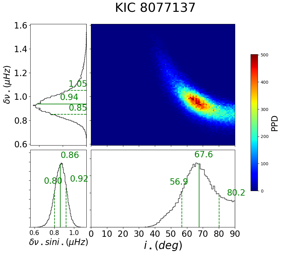
C.5 Kepler-128 (KOI-274, KIC 8077137)
C.6 Kepler-409 (KIC 9955598, KOI-1925)
C.7 KIC 7970740
C.8 KOI-268 (KIC 3425851)
C.9 KIC 6225718
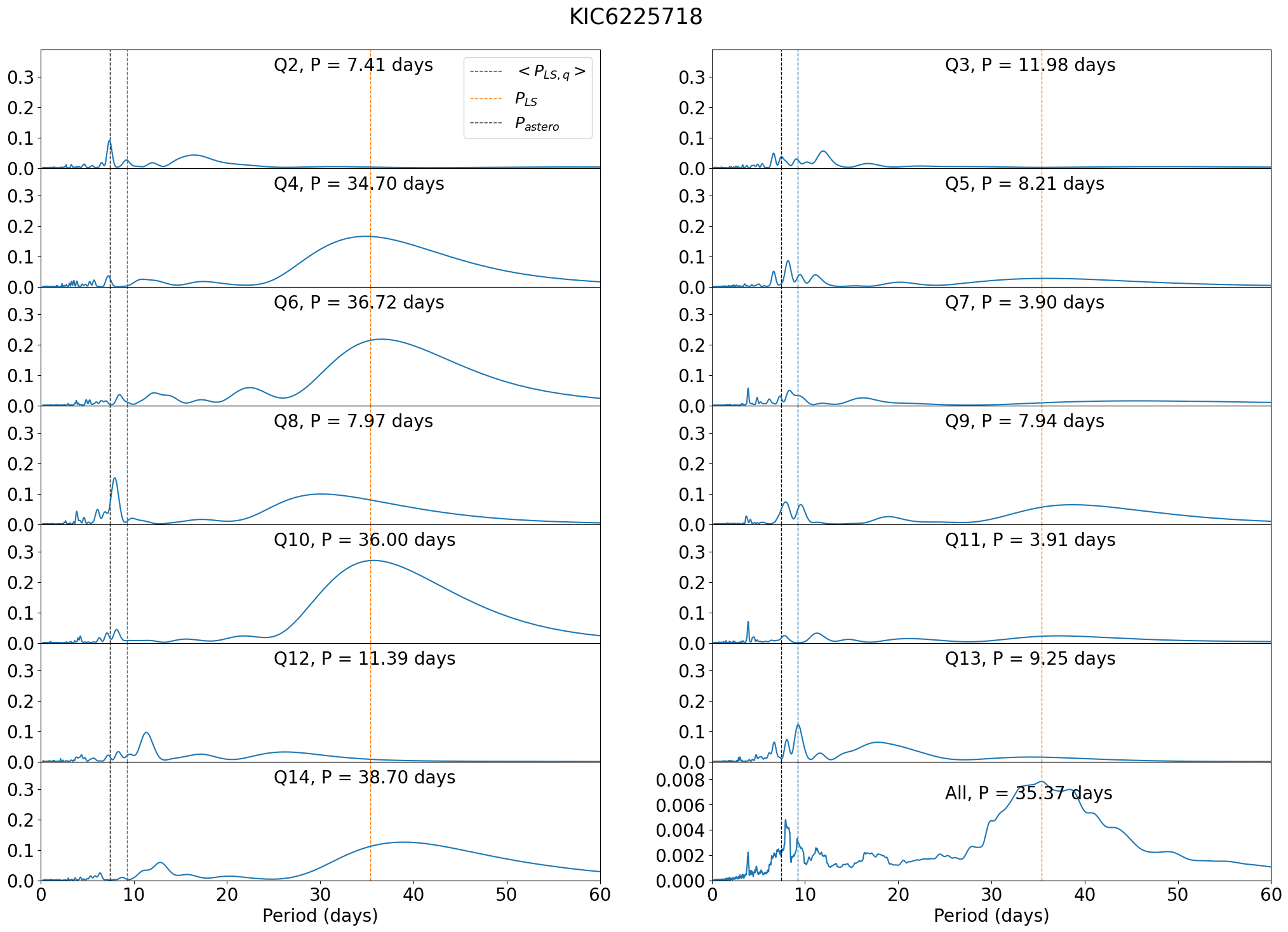
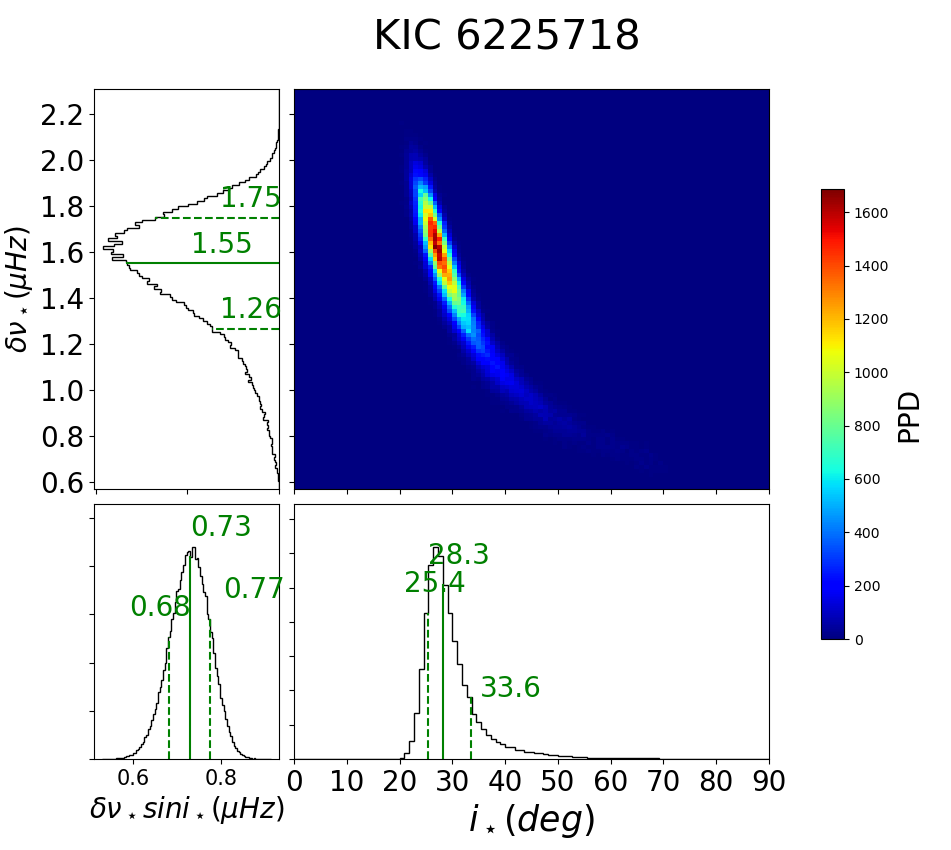
C.10 KIC 9965715
C.11 Kepler-2 (HAT-P-7, KOI-2, KIC 10666592)
C.12 Kepler-410 (KOI-42, KIC 8866102)
C.13 KOI-288 (KIC 9592705)
| \topruleKIC | KOIb | Kepler ID | RUWE | Ref. | |||||
|---|---|---|---|---|---|---|---|---|---|
| (Day) | (Day) | (Day) | (Day) | (Day) | |||||
| 11295426 | KOI-246 | Kepler-68 | 0.92 | 1 | |||||
| 8866102 | KOI-42 | Kepler-410 | 0.97 | 6 | |||||
| 10666592 | KOI-2 | HAT-P-7 | 0.98 | 4 | |||||
| 6278762 | KOI-3158 | Kepler-444 | 1 | 3 | |||||
| 3632418 | KOI-975 | Kepler-21 | 1.05 | 4 | |||||
| 9592705 | KOI-288 | 1.67 | 1 | ||||||
| 8554498 | KOI-5 | 4.89 | 1 | ||||||
| 9139151 | 0.8 | 2 | |||||||
| 9139163 | 0.93 | 2 | |||||||
| 3427720 | 1 | 2 | |||||||
| 9098294 | 1.64 | 5 | |||||||
| 8179536 | 1.8 | 5 | |||||||
| 8424992 | 2.08 | 5 | |||||||
| 12317678 | 3.93 | 5 | |||||||
| 7510397 | 4.28 | 2 | |||||||
| 4914923 | 5.14 | 5 | |||||||
| 9025370 | 5.16 | 2 | |||||||
| 1435467 | 5.73 | 5 | |||||||
| 10454113 | 5.96 | 5 | |||||||
| 7871531 | 9.7 | 5 | |||||||
| 6933899 | 13.14 | 5 | |||||||
| 8379927 | 32.79 | 2 |
-
a
Data adopted from Kamiaka et al. (2018)
- b
| \topruleKIC | KOIb | Kepler ID | Remark | |||||
|---|---|---|---|---|---|---|---|---|
| (Day) | (Day) | (Day) | (Day) | (Day) | ||||
| 11807274 | KOI-262 | Kepler - 50 | ||||||
| 5866724 | KOI-85 | Kepler - 65 | ||||||
| 6521045 | KOI-41 | Kepler - 100 | ||||||
| 8292840 | KOI-260 | Kepler - 126 | ||||||
| 10963065 | KOI-1612 | Kepler - 408 | ||||||
| 7670943 | KOI-269 | |||||||
| 9414417 | KOI-974 | |||||||
| 5773345 | ||||||||
| 7103006 | ||||||||
| 7206837 | ||||||||
| 7771282 | ||||||||
| 7940546 | ||||||||
| 9812850 | ||||||||
| 12009504 |
-
a
Data adopted from Kamiaka et al. (2018)
-
b
KOI number only available for systems with reported planet detection.
-
M
Suggested candidate of rotation period, (days). Target with multiple periodic component.
-
A
Suggested candidate of rotation period, (days). Target with abnormal quarter.
-
W
Targets with weak or no periodic signals.
| \topruleKIC | KOIb | Kepler ID | Remark | |||||
|---|---|---|---|---|---|---|---|---|
| (Day) | (Day) | (Day) | (Day) | (Day) | ||||
| 6196457 | KOI-285 | Kepler - 92 | ||||||
| 8494142 | KOI-370 | Kepler - 145 | ||||||
| 9955598 | KOI-1925 | Kepler - 409 | ||||||
| 3425851 | KOI-268 | |||||||
| 7970740 | ||||||||
| 9353712 | ||||||||
| 9410862 | ||||||||
| 10162436 | ||||||||
| 12258514 |
| \topruleKIC | KOIb | Kepler ID | Remark | |||||
|---|---|---|---|---|---|---|---|---|
| (Day) | (Day) | (Day) | (Day) | (Day) | ||||
| 4349452 | KOI-244 | Kepler - 25 | ||||||
| 3544595 | KOI-69 | Kepler - 93 | ||||||
| 8077137 | KOI-274 | Kepler - 128 | ||||||
| 2837475 | ||||||||
| 5184732 | ||||||||
| 6106415 | ||||||||
| 6116048 | ||||||||
| 6225718 | ||||||||
| 6508366 | ||||||||
| 6679371 | ||||||||
| 8006161 | ||||||||
| 8394589 | ||||||||
| 8694723 | ||||||||
| 9965715 | ||||||||
| 10079226 | ||||||||
| 10516096 | ||||||||
| 11081729 | ||||||||
| 11253226 | ||||||||
| 11772920 |
| \topruleKIC | KOIb | Kepler ID | Remark | |||||
|---|---|---|---|---|---|---|---|---|
| (Day) | (Day) | (Day) | (Day) | (Day) | ||||
| 11853905 | KOI-7 | Kepler - 4 | ||||||
| 11904151 | KOI-72 | Kepler - 10 | ||||||
| 11401755 | KOI-277 | Kepler - 36 | ||||||
| 8478994 | KOI-245 | Kepler - 37 | ||||||
| 8349582 | KOI-122 | Kepler - 95 | ||||||
| 4914423 | KOI-108 | Kepler - 103 | ||||||
| 5094751 | KOI-123 | Kepler - 109 | ||||||
| 10586004 | KOI-275 | Kepler - 129 | ||||||
| 11133306 | KOI-276 | Kepler - 509 | ||||||
| 4143755 | KOI-281 | Kepler - 510 | ||||||
| 4141376 | KOI-280 | Kepler - 1655 | ||||||
| 7296438 | KOI-364 | |||||||
| 3456181 | ||||||||
| 3656476 | ||||||||
| 3735871 | ||||||||
| 5950854 | ||||||||
| 6603624 | ||||||||
| 7106245 | ||||||||
| 7680114 | ||||||||
| 8150065 | ||||||||
| 8228742 | ||||||||
| 8760414 | ||||||||
| 8938364 | ||||||||
| 9206432 | ||||||||
| 10068307 | ||||||||
| 10644253 | ||||||||
| 10730618 | ||||||||
| 12069127 |
References
- Aguirre et al. (2017) Aguirre, V. S., Lund, M. N., Antia, H. M., et al. 2017, The Astrophysical Journal, 835, 173. https://iopscience.iop.org/article/10.3847/1538-4357/835/2/173https://iopscience.iop.org/article/10.3847/1538-4357/835/2/173/meta
- Aigrain et al. (2015) Aigrain, S., Llama, J., Ceillier, T., et al. 2015, MNRAS, 450, 3211. https://academic.oup.com/mnras/article-abstract/450/3/3211/1072143
- Appourchaux et al. (2008) Appourchaux, T., Michel, E., Auvergne, M., et al. 2008, A&A, 488, 705
- Astropy Collaboration et al. (2013) Astropy Collaboration, Robitaille, T. P., Tollerud, E. J., et al. 2013, A&A, 558, A33
- Astropy Collaboration et al. (2018) Astropy Collaboration, Price-Whelan, A. M., Sipőcz, B. M., et al. 2018, AJ, 156, 123
- Barclay et al. (2013) Barclay, T., Rowe, J. F., Lissauer, J. J., et al. 2013, Nature, 494, 452. http://arxiv.org/abs/1301.0842
- Benomar et al. (2014) Benomar, O., Masuda, K., Shibahashi, H., & Suto, Y. 2014, PASJ, 66, 94
- Benomar et al. (2018) Benomar, O., Bazot, M., Nielsen, M. B., et al. 2018, Science, 361, 1231
- Brasseur et al. (2019) Brasseur, C. E., Phillip, C., Fleming, S. W., Mullally, S. E., & White, R. L. 2019, Astrocut: Tools for creating cutouts of TESS images, Astrophysics Source Code Library, record ascl:1905.007, ascl:1905.007
- Brewer et al. (2016) Brewer, J. M., Fischer, D. A., Valenti, J. A., & Piskunov, N. 2016, The Astrophysical Journal Supplement Series, 225, 32. https://doi.org/10.3847/0067-0049/225/2/32
- Bruntt et al. (2012) Bruntt, H., Basu, S., Smalley, B., et al. 2012, MNRAS, 423, 122
- Campante et al. (2016) Campante, T. L., Lund, M. N., Kuszlewicz, J. S., et al. 2016, ApJ, 819, 85
- Ceillier et al. (2016) Ceillier, T., Van Saders, J., García, R. A., et al. 2016, MNRAS, 456, 119. http://archive.stsci.edu/kepler/koi/search.php
- Ceillier et al. (2017) Ceillier, T., Tayar, J., Mathur, S., et al. 2017, A&A, 605, A111. https://doi.org/10.1051/0004-6361/201629884
- Chaplin et al. (2013) Chaplin, W. J., Sanchis-Ojeda, R., Campante, T. L., et al. 2013, ApJ, 766, 101
- Chowdhury et al. (2018) Chowdhury, S., Joshi, S., Engelbrecht, C. A., et al. 2018, Ap&SS, 363, 260
- Donahue et al. (1996) Donahue, R. A., Saar, S. H., & Baliunas, S. L. 1996, ApJ, 466, 384
- Evans (2018) Evans, D. F. 2018, Research Notes of the American Astronomical Society, 2, 20
- Eylen et al. (2014) Eylen, V. V., Lund, M. N., Aguirre, V. S., et al. 2014, The Astrophysical Journal, 782, 14. https://doi.org/10.1088/0004-637x/782/1/14
- Fabricius et al. (2021) Fabricius, C., Luri, X., Arenou, F., et al. 2021, A&A, 649, A5. https://doi.org/10.1051/0004-6361/202039834
- García et al. (2019) García, R. A., Ballot, J., García, R. A., & Ballot, J. 2019, Living Reviews in Solar Physics, 16, 4. http://irfu.cea.fr/Sap/
- García et al. (2013) García, R. A., Ceillier, T., Mathur, S., & Salabert, D. 2013, in Astronomical Society of the Pacific Conference Series, Vol. 479, Progress in Physics of the Sun and Stars: A New Era in Helio- and Asteroseismology, ed. H. Shibahashi & A. E. Lynas-Gray, 129
- García et al. (2014) García, R. A., Ceillier, T., Salabert, D., et al. 2014, A&A, 572, A34
- Ginsburg et al. (2019) Ginsburg, A., Sipőcz, B. M., Brasseur, C. E., et al. 2019, AJ, 157, 98
- Gizon & Solanki (2003) Gizon, L., & Solanki, S. K. 2003, ApJ, 589, 1009
- Gizon & Solanki (2004) —. 2004, Sol. Phys., 220, 169
- Hall et al. (2021) Hall, O. J., Davies, G. R., van Saders, J., et al. 2021, Nature Astronomy, 5, 707
- Hartmann & Noyes (1987) Hartmann, L. W., & Noyes, R. W. 1987, ARA&A, 25, 271
- Hirano et al. (2012) Hirano, T., Sanchis-Ojeda, R., Takeda, Y., et al. 2012, ApJ, 756, 66
- Howard & Harvey (1970) Howard, R., & Harvey, J. 1970, Sol. Phys., 12, 23
- Huber et al. (2013) Huber, D., Chaplin, W. J., Christensen-Dalsgaard, J., et al. 2013, ApJ, 767, 127
- Hunter (2007) Hunter, J. D. 2007, Computing in Science & Engineering, 9, 90
- Kamiaka et al. (2018) Kamiaka, S., Benomar, O., & Suto, Y. 2018, Monthly Notices of the Royal Astronomical Society, 479, 391. https://academic.oup.com/mnras/advance-article/doi/10.1093/mnras/sty1358/5001890
- Kamiaka et al. (2019) Kamiaka, S., Benomar, O., Suto, Y., et al. 2019, AJ, 157, 137
- Karoff et al. (2013) Karoff, C., Metcalfe, T. S., Chaplin, W. J., et al. 2013, MNRAS, 433, 3227
- Kepler Eclipsing Binary working group (2019) Kepler Eclipsing Binary working group. 2019, Kepler Eclipsing Binary catalogue, v3rd Revsion; Last Accessed: 2021-11-14, , . http://keplerebs.villanova.edu
- Kepler Mission (2019) Kepler Mission. 2019, Kepler Stellar Properties Table, vVersion 2; Last Accessed: 2021-10-06, IPAC, doi:10.26133/NEA6. https://catcopy.ipac.caltech.edu/dois/doi.php?id=10.26133/NEA6
- Kjeldsen & Bedding (1995) Kjeldsen, H., & Bedding, T. R. 1995, A&A, 293, 87
- Kraft (1967) Kraft, R. P. 1967, ApJ, 150, 551
- Ledoux (1951) Ledoux, P. 1951, ApJ, 114, 373
- Lightkurve Collaboration et al. (2018) Lightkurve Collaboration, Cardoso, J. V. d. M., Hedges, C., et al. 2018, Lightkurve: Kepler and TESS time series analysis in Python, Astrophysics Source Code Library, ascl:1812.013
- Lillo-Box et al. (2014) Lillo-Box, J., Barrado, D., & Bouy, H. 2014, A&A, 566, A103. https://doi.org/10.1051/0004-6361/201423497
- Lomb (1976) Lomb, N. R. 1976, Astrophysics and Space Science, 39, 447. http://dx.doi.org/10.1007/BF00648343
- Lund et al. (2017) Lund, M. N., Silva Aguirre, V., Davies, G. R., et al. 2017, ApJ, 835, 172
- Mabelcalim (2014) Mabelcalim. 2014, waipy, https://github.com/mabelcalim/waipy, GitHub
- Marcy et al. (2014) Marcy, G. W., Isaacson, H., Howard, A. W., et al. 2014, ApJS, 210, 20
- McQuillan et al. (2013) McQuillan, A., Mazeh, T., & Aigrain, S. 2013, The Astrophysical Journal Letters, 775, L11
- McQuillan et al. (2014) McQuillan, A., Mazeh, T., & Aigrain, S. 2014, ApJS, 211, 24
- Molenda-Żakowicz et al. (2013) Molenda-Żakowicz, J., Sousa, S. G., Frasca, A., et al. 2013, MNRAS, 434, 1422
- Mosser et al. (2013) Mosser, B., Michel, E., Belkacem, K., et al. 2013, A&A, 550, A126
- Nielsen et al. (2013) Nielsen, M. B., Gizon, L., Schunker, H., & Karoff, C. 2013, A&A, 557, 10. http://cdsarc.u-strasbg.fr/viz-bin/qcat?J/A+A/557/L10
- Nielsen et al. (2015) Nielsen, M. B., Schunker, H., Gizon, L., & Ball, W. H. 2015, Astronomy & Astrophysics, 582, A10. https://www.aanda.org/articles/aa/full{_}html/2015/10/aa26615-15/aa26615-15.htmlhttps://www.aanda.org/articles/aa/abs/2015/10/aa26615-15/aa26615-15.html
- Paxton et al. (2011) Paxton, B., Bildsten, L., Dotter, A., et al. 2011, ApJS, 192, 3
- Petigura et al. (2017) Petigura, E. A., Howard, A. W., Marcy, G. W., et al. 2017, AJ, 154, 107
- Pinsonneault et al. (2012) Pinsonneault, M. H., An, D., Molenda-Żakowicz, J., et al. 2012, ApJS, 199, 30
- Rauer et al. (2014) Rauer, H., Catala, C., Aerts, C., et al. 2014, Experimental Astronomy, 38, 249
- Reiners & Schmitt (2003) Reiners, A., & Schmitt, J. H. M. M. 2003, A&A, 412, 813
- Reinhold & Gizon (2015) Reinhold, T., & Gizon, L. 2015, Astronomy & Astrophysics, 583, A65. http://www.aanda.org/10.1051/0004-6361/201526216
- Reinhold & Reiners (2013) Reinhold, T., & Reiners, A. 2013, Astronomy & Astrophysics, 557, A11. http://www.aanda.org/10.1051/0004-6361/201321161
- Reinhold et al. (2020) Reinhold, T., Shapiro, A. I., Solanki, S. K., et al. 2020, Science, 368, 518. https://www.science.org/doi/abs/10.1126/science.aay3821
- Santos et al. (2017) Santos, A. R. G., Cunha, M. S., Avelino, P. P., García, R. A., & Mathur, S. 2017, A&A, 599, A1. https://doi.org/10.1051/0004-6361/201629923
- Santos et al. (2019) Santos, A. R. G., García, R. A., Mathur, S., et al. 2019, The Astrophysical Journal Supplement Series, 244, 21. https://doi.org/10.3847/1538-4365/ab3b56
- Scargle (1982) Scargle, J. D. 1982, ApJ, 263, 835
- Schou et al. (1998) Schou, J., Antia, H. M., Basu, S., et al. 1998, ApJ, 505, 390
- Skumanich (1972) Skumanich, A. 1972, apj, 171, 565
- Stumpe et al. (2014) Stumpe, M. C., Smith, J. C., Catanzarite, J. H., et al. 2014, Publications of the Astronomical Society of the Pacific, 126, 100. https://doi.org/10.1086%2F674989
- Suto et al. (2019) Suto, Y., Kamiaka, S., & Benomar, O. 2019, AJ, 157, 172
- Suto et al. (2022) Suto, Y., Sasaki, S., Nakagawa, Y., & Benomar, O. 2022, arXiv e-prints, arXiv:2205.04836
- Tassoul (1980) Tassoul, M. 1980, ApJS, 43, 469
- Thompson et al. (2003) Thompson, M. J., Christensen-Dalsgaard, J., Miesch, M. S., & Toomre, J. 2003, ARA&A, 41, 599
- Torrence & Compo (1998) Torrence, C., & Compo, G. P. 1998, Bulletin of the American Meteorological Society, 79, 61. http://paos.colorado.edu/research/wavelets/bams{_}79{_}01{_}0061.pdfhttp://journals.ametsoc.org/doi/abs/10.1175/1520-0477{%}281998{%}29079{%}3C0061{%}3AAPGTWA{%}3E2.0.CO{%}3B2
- Van Eylen et al. (2014) Van Eylen, V., Lund, M. N., Silva Aguirre, V., et al. 2014, ApJ, 782, 14
- van Saders et al. (2016) van Saders, J., Ceillier, T., Metcalfe, T., et al. 2016, nat, 529, 181
- VanderPlas (2018) VanderPlas, J. T. 2018, The Astrophysical Journal Supplement Series, 236, 16. http://stacks.iop.org/0067-0049/236/i=1/a=16?key=crossref.2d79c6c284b1df1e8149df501e36ea6bhttps://iopscience.iop.org/article/10.3847/1538-4365/aab766
- Wes McKinney (2010) Wes McKinney. 2010, in Proceedings of the 9th Python in Science Conference, ed. Stéfan van der Walt & Jarrod Millman, 56 – 61
- Winn et al. (2010) Winn, J. N., Fabrycky, D., Albrecht, S., & Johnson, J. A. 2010, ApJ, 718, L145
- Winn & Fabrycky (2015) Winn, J. N., & Fabrycky, D. C. 2015, ARA&A, 53, 409
- Wolniewicz et al. (2021) Wolniewicz, L. M., Berger, T. A., & Huber, D. 2021, The Astronomical Journal, 161, 231. https://doi.org/10.3847/1538-3881/abee1d
- Zechmeister & Kürster (2009) Zechmeister, M., & Kürster, M. 2009, Astronomy & Astrophysics, 496, 577. https://www.aanda.org/articles/aa/pdf/2009/11/aa11296-08.pdfhttp://www.aanda.org/10.1051/0004-6361:200811296