Metastability in Stochastic Replicator Dynamics
Abstract: We consider a novel model of stochastic replicator dynamics for potential games that converts to a Langevin equation on a sphere after a change of variables. This is distinct from the models of stochastic replicator dynamics studied earlier. In particular, it is ill-posed due to non-uniqueness of solutions, but is amenable to a natural selection principle that picks a unique solution. The model allows us to make specific statements regarding metastable states such as small noise asymptotics for mean exit times from their domain of attraction, and quasi-stationary measures. We illustrate the general results by specializing them to replicator
dynamics on graphs and demonstrate that the numerical experiments support theoretical predictions.
Key words: stochastic replicator dynamics; Langevin equation on sphere; metastable states; intermittency; small noise asymptotics; mean exit time; quasi-stationary distributions
MSC: Primary: 91A22 Secondary: 91A25; 60H10; 34F05
1 Introduction
This work is motivated by the studies on intermittent dynamics of complex large-scale systems [23], [54], [62]. We model the dynamics of a large-scale complex system by replicator dynamics with noise, a classical model in evolutionary biology. Replicator dynamics per se is an extensively studied dynamics [36], [55], [65]. Its noisy version is much less so. In their seminal work, Foster and Young [27] considered small noise asymptotics of the stationary regime of replicator dynamics perturbed by small noise and used it to formulate the notion of stochastically stable equilibria, i.e., Nash equilibria that arise as limit(s) when noise is reduced to nil in the stationary regime. This provided a selection principle for Nash equilibria (see also [67]). This is of interest because multiple Nash equilibria is a commonplace situation and one does need a selection principle of some sort to narrow down the relevant possibilities. While early work in this direction was based on static refinements of the notion of Nash equilibrium [34], [64], later developments sought dynamic models where some Nash equilibria would naturally emerge as stable equilibria of the dynamics [30], [55]. This, however, only partially solves the problem, because, as mentioned above, even stable equilibria can be many. The important observation of Foster and Young was that only some of them may be stable under stochastic perturbations in the stationary regime, a physically relevant concern. (See also [45], [47] for interesting takes on behavioral aspects of noise and [14], [25], [32] for connections with finite population models. The general philosophy of using small noise limits for selection principles in ill-posed dynamics has been attributed to Kolmogorov in [26], p. 626.)
The elegant machinery for small noise asymptotics of noise-perturbed dynamics due to Freidlin and Wentzell [28] gives us a handle to tag these equilibria in a precise manner, viz., as minimizers of the so-called Freidlin-Wentzell potential associated with the process. This is precisely what Foster and Young did. But this still leaves wide open the issue of metastability, a familiar phenomenon in statistical physics [18]. Well known examples are supercooled water, air supersaturated with vapor, etc., which on suitable perturbation result in resp. freezing (ice) or condensation (rain). There have been various analytic approaches to quantitative analysis of metastability, see the opening chapters of [18] for a succinct overview and historical account. Our approach follows that formulated by Kramers [43] who viewed them as equilibria of a gradient system perturbed by noise. The later seminal work of Freidlin and Wentzell [28] generalized this viewpoint considerably, encompassing non-gradient systems and attractors more general than equilibria. In this viewpoint, metastable states are stable equilibria for the deterministic dynamics that will not arise as a small noise limit in the stationary regime, but are still important because of the celebrated quasi-stationarity phenomenon [24]: the process may spend long time near such equilibria on time scales relevant to us before approaching true stationarity. An alternative though related viewpoint is that these are equilibria which the system gets out of when given a perturbation of a certain magnitude. In case of gradient systems, the size of the perturbation will be related to the barrier between the current metastable state and its neighboring equilibria as captured by the optimal trajectory (i.e., one minimizing the ‘rate function’ of the associated large deviations) needed to climb in order to get out of the current ‘valley’ or domain of attraction for the noiseless system. Analogous ideas exist for non-gradient systems in terms of the aforementioned Freidlin-Wentzell potential. See [50] for an extensive account of this approach and [8] for some recent developments.
A related phenomenon is that of intermittency, where one sees the process spend nontrivial time in the neighborhood of a succession of stable equilibria with abrupt noise-induced episodic transitions between them (see [23], [54], [62] for examples from physics and biology). This will be the case when the noise is small but not too small so that these transitions occur on an observable time scale. This should not be confused with the phenomenon of intermittency in chaotic systems wherein a deterministic dynamics exhibits long periods of slow variation punctuated by spurts of chaotic behavior [51]. The analysis of Fredlin-Wentzell shows that the process may be viewed as approximating a Markov chain over stable equilibria (more generally, stable attractors) with transition times and probabilities characterized in terms of a suitable ‘action’ functional [28]. The small noise asymptotics gives a feel for the noise levels for which one expects intermittency instead of quasi-stationarity.
In view of the foregoing one important numerical quantity associated with such a metastable equilibrium is the mean exit time from its domain of attraction, or rather, the scaling properties thereof in the small noise limit. Our aim here is to present one such result in the case of replicator dynamics with potential. While bounds on this quantity are available [39] for the specific model considered by [19], [29], we give a finer result using the Freidlin–Wentzell theory [28]. A highlight of our approach is that it is based on an interesting connection between replicator dynamics for potential games and gradient descent on a sphere, a compact manifold without boundary which allows the application of Freidlin-Wentzell theory without facing the complications encountered by Foster and Young in doing so - see, e.g., the correction note to [27]. It provides an alternative treatment to such issues distinct from that of [39] that is simpler in many ways. We also gain some important insights into quasi-stationary distributions.
In related works [57], [58], replicator dynamics is viewed as a large population ‘mean field’ limit of finite population stochastic models (see, e.g., [16]) and large deviations phenomena in the stationary regime are analyzed. Our emphasis, in contrast, is on quasi-stationary behavior. As noted in [52], the quasi-stationary behavior is closely associated with the ‘hardness’ of the underlying optimization problem of minimizing the potential. This also reflects in the slow convergence of the simulated annealing algorithm for non-convex potentials, which is a time-inhomogeneous stochastic gradient descent with slowly decreasing noise [2], [20], [21]. Other related works on asymptotic behavior of noisy replicator dynamics are [35], [48], [49]. Mathematically, what sets our model apart is a diffusion matrix involving in non-diagonal positions square-roots of state variables that puts it beyond available well-posedness results for stochastic differential equations. In fact it is ill-posed due to non-uniqueness of solutions, thus we need to resort to a well motivated selection principle to pick a unique choice.
To summarize, the main contributions of the present work are: (a) we introduce a new variant of the stochastic replicator dynamics, which in particular allows us to work around the problem of “corners” in [27], (b) we propose a transformation that converts our model to a Langevin equation on a sphere; (c) a selection principle to overcome the ill-posedness of the original model is then proposed; (c) we characterize for our model the exit time asymptotics from metastable states and also characterize its quasi-stationary distributions; (d) we apply these general results to study the intermittent behaviour of large complex systems described by graphs; and finally, (e) we illustrate main theoretical findings by numerical examples.
The article is organized as follows. The next section introduces our model of stochastic replicator dynamics
and discusses in detail its relationship to other stochastic replicator dynamics in literature.
Section 3 uses a transformation to map it into the Langevin equation on a sphere and exploits the structure therein to analyze the small noise asymptotics. Section 4 specializes the results to the case of quadratic
potentials on graphs and makes some relevant observations for this special case which has important applications
such as the study of the intermittent behaviour in complex large-scale systems [23], [54],
[62] and clique detection problem [4], [10], [11], [12].
Section 5 presents some numerical experiments to support the theoretical findings.
We conclude the paper with suggestions for future research in Section 6.
2 Stochastic replicator dynamics with potential
Replicator dynamics, introduced by Taylor and Jonker [61], is a model for behavior adjustment of population games, i.e., a game theoretic scenario in which we analyze collective behavior of a population of agents belonging to certain ‘types’ or ‘species’ in conflict situation, retaining only their species/type tag and erasing their individual identity. This is because their strategic behavior is dictated by the type, as also the environment they face is dictated by the collective sizes and strategic behavior of other types. The origin of this particular dynamics of population games (among many, see [55] for an extensive treatment) lies in models of Darwinian evolution in biology [36]. Issues of interest typically are convergence to an equilibrium behavior, persistence or non-extinction, etc. Among others, one very significant outcome of this theory is the link between the so-called evolutionarily stable states, a biologically relevant equilibrium notion introduced by John Maynard Smith, and asymptotically stable equilibrium points of replicator dynamics. See [36], [55], [65] for a detailed treatment. We further restrict to a special subclass of these, viz., potential games wherein the payoff function is restricted to be of a particular form, see again [55] for an extensive account of the deterministic case. This subclass, defined later, is much more analytically amenable and has important applications, e.g., in congestion games.
Our focus will be on stochastic replicator dynamics with potential. We begin with a motivating example of deterministic replicator dynamics with linear payoffs and then introduce the more general paradigm.
2.1 Deterministic replicator dynamics and potential games
Let
denote the -dimensional probability simplex. The deterministic replicator dynamics with linear payoffs is the following differential equation in :
| (1) |
where the matrix is a payoff matrix, i.e., the th element of is the payoff to species when the population profile is . We assume that is symmetric.
In evolutionary biology, is interpreted as the fraction of species in the population, thus being the overall population profile. The quantity is the payoff for species at time when the population profile is . The quantity is then the average payoff for the population at time . Thus, the population share of species waxes or wanes at a rate proportional to its excess, resp., deficit of payoff over the population average. The standard equilibrium notion for population game is that of Nash equilibrium defined as follows: is a Nash equilibrium if . An analogous definition is also used when is replaced by a nonlinear payoff function , as we do a bit later. A population profile is evolutionarily stable if for sufficiently close to . Then Nash equilibria are the equilibrium points of the deterministic replicator dynamics and the evolutionarily stable states are asymptotically stable equilibria, though neither converse holds (see e.g., [36], [55], [65].) While natural and appealing, the problem with stopping with these definitions is that of multiple equilibria as already mentioned, calling for a selection principle which stochastic replicator dynamics tries to provide.
Equation (1) can be written in the following matrix-vector form
| (2) |
where we introduce the notation:
-
•
diag for is the diagonal matrix whose th diagonal entry is and,
-
•
1 is the constant vector of all ’s.
Then, we observe that (2) is a particular case of
| (3) |
with . Given , the right hand side summed over its components adds to zero, implying that a constant on . Since the th component of this dynamics is of the form
for a suitably defined , its solution is of the form , which together with the preceding observation implies that the simplex
of probability vectors is invariant under (3). In fact, it is also clear that if a component is zero for some , it is always so - this is immediate from the uniqueness of solutions. So the faces of are also invariant under (3) and the trajectory in any face cannot enter a lower dimensional face in finite time.
For a replicator dynamics of form (3), is said to be its associated potential function, assumed continuously differentiable (which it indeed is in our case). Then it is easy to check (see [65], p. 110, or [55], Section 7.1, for a more general statement and an extensive account of the deterministic dynamics (3)) that
with equality on the set
This includes the critical points of . Then the above inequality implies that is non-decreasing along any trajectory of (3) and strictly increasing outside . This ensures convergence of all trajectories to . Note that is specified by a set of nonlinear equations. We shall assume that it is a union of lower dimensional manifolds, which can usually be verified by using the implicit function theorem. In that case, it is clear that for any points in other than the local maxima of , there will be a direction transversal to along which must increase (otherwise it would have been a local maximum). (See [55], p. 273, for a related discussion.) Thus serves as a Liapunov function for (3), implying convergence to the local maxima of for generic (i.e., belonging to an open dense set) initial conditions. Then (2) is a special case with . The entire development to follow goes through for general continuously differentiable , so we shall consider this general case henceforth.
2.2 Stochastic replicator dynamics
The stochastic or noise-perturbed replicator dynamics is the following stochastic differential equation in :
| (4) |
where
-
•
is the standard -dimensional Wiener process;
-
•
is a small parameter;
-
•
is a continuously differentiable potential function and is a payoff to species when the population profile is ;
-
•
with the th row thereof.
In order that
truly evolves in a probability simplex, we require that
| (5) |
In [27], there is an additional requirement of continuity on which ensures well-posedness of (4). It is worth noting that in the model we shall propose, we do away with this: our choice is continuous in the interior of , but singular at its boundaries. The product is, however, continuous, but not Lipschitz at the boundary. Not surprisingly, well-posedness fails - the solutions are not unique. Note also that our state space is the simplex and hence the above applies only to , the rest of is irrelevant. Except for the aforementioned regularity requirement, our model does fit the Foster-Young framework [27] in its overall structure.
In [27], the noise component of (4) is attributed to mutation and migration. The latter is also used to justify a reflected diffusion formulation. The continuity assumption on suffices to ensure the existence of a weak solution, but since (5) implies in particular that the ensuing diffusion is not uniformly nondegenerate, some additional care is needed to ensure uniqueness. For example, Lipschitz condition would suffice. That said, the variant we introduce later does away with the uniqueness requirement and opts for a selection principle instead – more on that later.
The standard framework for analyzing diffusions described by stochastic differential equations that allows one to handle a sufficiently rich class of problems is the Stroock-Varadhan martingale formulation, which is a ‘weak’ formulation as opposed to the original Ito formulation in terms of ‘strong’ solutions. In this formulation, one is given a densely defined local333Extensions to non-local operators for, e.g., discontinuous processes, exist. operator on the space of bounded continuous functions on the state space, with suitable technical conditions. By a solution for a given initial condition , one means a process defined on some probability space so that
is a martingale with respect to the natural filtration of -fields generated by , for bounded continuous on the state space in the domain of . The problem is well-posed if this process is unique in law for each and the resulting laws, tagged by , satisfy the Chapman-Kolmogorov equation. In case of non-uniqueness, under mild continuity requirements one has a nonempty compact family of solutions for each . A selection principle then entails picking one solution per so that the Chapman-Kolmogorov equation is satisfied. The classic work in this direction is that of [44], which, however, has limitations that we shall point out later. We shall employ a different selection principle suited for our purposes, which can be developed in a more principled manner. In particular, it is in the spirit of the Kolmogorov philosophy alluded to in the introduction and thus well-motivated for game theoretic application, somewhat in the spirit of ‘trembling hand perfect equilibria’, a refinement of Nash equilibria in static framework defined in terms of stability under random perturbations (see, e.g., [31], [67]).
On purely mathematical grounds, an advantage of our formulation is that it is the natural extension of deterministic replicator dynamics for which the celebrated coordinate transformation of [3], [59] that maps deterministic replicator dynamics for potential games to a gradient flow on sphere, extends to the stochastic case. In fact we exploit this fact in a major way in our analysis. Furthermore, it avoids artificial restrictions on the state space in the passage from deterministic to stochastic and when converted to gradient dynamics on sphere, it allows for seamless conversion from Ito to Stratonovich form and back due to absence of a correction term, allowing either formulation to be used according to convenience. All these issues are explained later in this work, as they require some preparatory material.
Note that is an -dimensional manifold with boundary and corners. This presented some problem in the analysis of small noise limit for the noisy replicator dynamics in [27], which required the authors to use the extension of the Freidlin-Wentzell theory due to Anderson and Orey [5] that handles such cases (see the correction note to [27]). We propose here a simpler route by confining ourselves to an alternative of , which we motivate next.
Let denote the payoff accumulation rate for species when the population profile is . Consider first the unnormalized population dynamics for the th species given by
| (6) |
where is the population of species at time and
| (7) |
is resp. the total population at time and the population share (as a fraction of total population) of species at time ( by convention). We assume to be Lipschitz so that well-posedness of the corresponding deterministic dynamics
in is not an issue. We do not consider the well-posedness of (6) which is a degenerate diffusion with a non-Lipschitz diffusion coefficient. But we do so later in this article for the stochastic replicator dynamics we get after normalization. Our point of departure from earlier models of stochastic replicator dynamics is the stochastic forcing term, which is to be interpreted as follows. The noise seen by the th species as a whole has incremental variance proportional to its own population and the population of each of other species (inclusive of itself, because the ‘infinitesimal’ agents of a species also interact with other such agents in the same species), summed over the latter. In other words, it is where is the time increment. This is motivated by the fact that the variance of a sum of i.i.d. random variables scales linearly with the number thereof, therefore the net variance in the stochastic interaction of two populations should be proportional to the product of their respective sizes, assuming that each ‘infinitesimal’ interaction between two agents picks independent noise. This leads to the noise term above where is a scale parameter and are independent standard Brownian motions. This is in contrast to the earlier models that add noise directly to the normalized (replicator) dynamics or to the payoffs in the unnormalized population dynamics - the noise is now attached to each (infinitesimal) interaction episode and not to any overall gross feature such as the net payoff. This makes ours a game theoretically distinct model.
Lemma 2.1 The process satisfies
| (9) | |||||
This will be the stochastic replicator dynamics we analyze. Note that the diffusion coefficients in
are not Lipschitz near the boundary of , so the standard proof of well-posedness of stochastic differential equations with Lipschitz coefficients does not apply. Even the celebrated work of Watanabe and Yamada [66] that establishes well-posedness under weaker (e.g., certain Hölder continuity) conditions does not apply because of the presence of non-diagonal terms. In fact (9) is not well-posed - its solution is not unique as we shall see later. We shall therefore propose a selection principle to choose a specific solution as the ‘natural’ or ‘physical’ solution. For the time being, note that in the notation of (4),
or,
where is the Kronecker delta. Letting , we have for as desired, because is the projection to the space .
We take up the ill-posedness issues and subsequent analysis of this dynamics in the next section.
As was already mentioned, our model is a particular instance of a general formulation in [27], but with different regularity conditions. We now compare it with other models somewhat similar in spirit. An important predecessor is the work of Fudenberg and Harris [29] mentioned earlier, followed by a series of works [19, 39, 35, 42]. In that model, they begin with a ‘raw’ (i.e., unnormalized) growth model for the populations with the payoffs perturbed by scaled Brownian noise, in the spirit of the classical derivation of the deterministic replicator dynamics [65]. This leads to the equation (6) modified by using geometric Brownian motion as follows:
When the Ito transformation is applied to obtain the s.d.e. for the population fractions , this leads to
Note that new terms appear in the deterministic part.
Recently, Mertikopoulos and Viossat [49] proposed to introduce directly the geometric-type Brownian motion in the s.d.e. for the population fractions, which resulted in the following version of the stochastic replicator dynamics:
with the diffusion coefficients being Lipschitz. This is a well-posed stochastic differential equation unlike ours and while also a particular case of [27], it is qualitatively different in various aspects as will become apparent as we proceed. Most importantly, their model shares with classical models the feature that no species can become extinct (i.e., the corresponding component hit zero) in finite time, whereas ours can, and get reflected, implying fresh arrivals of the species into the system. Also, in [49] the authors address issues different from the ones we do.
3 A transformation of the state space and analysis of metastability
Our first objective is to overcome the difficulty in treating corners in [27] by using dynamics (9).
This is achieved through a change of variable . For the -dimensional sphere, define . For the deterministic o.d.e. (3), this change of variable leads to
| (10) |
where denotes the projected gradient operator that gives gradient in the tangent space of . The new dynamics (10) is then nothing but gradient ascent on , a compact manifold without boundary.
This transformation goes back to [3], [59], see [56] for a recent treatment which also discusses other related projection dynamics. The dynamics (10) as defined above is well defined on the entire , not just on its positive orthant. Setting establishes a one-to-one correspondence of each orthant of with . Note that all local maxima, resp. minima of in get mapped to local maxima, resp. minima of in a one to many map. At the boundary of the orthants, the vector fields on either side will exhibit a mirror symmetry with respect to this boundary because of the nature of our transformation, in particular, the component of the driving vector field normal to the boundary will be symmetric across the boundary and being continuous, must vanish at the boundary. As observed earlier, the replicator dynamics in a face of does not reach a lower dimensional face in finite time. The same will be true for the gradient ascent above vis-a-vis boundaries of orthants, because the normal component of the above vector field vanishes at the boundary, slowing down its approach to the boundary. This, however, is not the case for the stochastic version as we shall see later.
Consider now the process satisfying
| (11) | |||||
| (12) |
where ‘’ denotes the Stratonovich integral and
is a Brownian motion in . (This is a consequence of the fact that for is a projection to the tangent space of at . Note that this is an extrinsic description of which requires that be viewed as a manifold embedded in .)
The state space of is the entire , with full support because as a diffusion in , is non-degenerate. In particular, unlike the deterministic case, the trajectories do cross over from one orthant to another because of the Brownian component: at a point on the boundary, the normal component of the gradient drift is zero, so the normal component of the diffusion is a pure Brownian motion, implying that it will be on either side of the boundary with probability one in an arbitrarily small time interval.
Proof: The Ito to Stratonovich conversion of a vector s.d.e.
written componentwise as
goes as follows. For any twice continuously differentiable , we have by Ito formula,
and
Hence
Applying this to (11), we have
| (14) |
which proves the claim.
Remark: Ito and Stratonovich444The work [42] suggests the use of Stratonovich formulation for a different reason, viz., that it correctly captures the limiting behavior of ordinary differential equations with rapidly varying random right hand side. An older work [63], however, is critical of Stratonovich formulation because it misses out on some biologically relevant or realistic aspects, but as our main motivation is not from biology, we do not address these issues. See [37] for general background on diffusions on manifolds. integrals are certainly not always identical and there can be an error term. The lemma states that this term is zero for us. We emphasize this need not always be the case. The reason it works out for us is that our stochastic gradient dynamics on sphere is driven by a pure Brownian motion for which the diffusion coefficient is identity and therefore there is no Stratonovich correction. Our aim in stating (11) in Stratonovich form is purely to avoid technicalities in handling the Ito version (13) in the manifold framework. The advantage of Stratonovich formulation is that it is more amenable to smooth coordinate transformations: even though we eventually work on the probability simplex, a compact manifold with boundary that admits a single local chart for the entire manifold, our passage to it is via a stochastic differential equation on a sphere, a compact manifold without boundary that does not admit a single local chart.
We may identify a vector in with in its positive orthant. Under this equivalence relation, the quotient space is the positive orthant of and maps to a reflected diffusion in . This requires that we modify (9)-(9) to include a boundary term to account for the reflection, specifically a bounded variation increasing process supported on the boundary that confines the original process to the prescribed domain. We also need to specify a direction of reflection. This is because the Brownian and hence the diffusion trajectory is non-differentiable everywhere with probability one, therefore its direction of reflection on the boundary cannot be defined in a conventional manner. As in the case of simple reflected Brownian motion, pure reflection across a codimension one smooth surface entails normal reflection, as can be justified also by symmetry considerations: is the mirror image of across the plane and the line joining the two is normal to this plane. The other specification needed is whether the reflection is instantaneous or ‘sticky’. Our definition of implies instantaneous reflection. Both these specifications are achieved by adding to the dynamics a bounded variation process which confines the process to the desired domain while respecting the prescribed reflection direction. We describe this in detail below. This material is standard and a nice exposition can be found in [38]. Thus, if is a reflected diffusion with normal reflection in , it satisfies
| (15) |
where is a process (called the ‘local time’ at the boundary) satisfying:
-
1.
the zero vector;
-
2.
If denotes the total variation of on , then (i.e., it is a bounded variation process) and
(i.e., it increases only when , implying instantaneous reflection);
-
3.
For , let the inward normal if belongs to one of the primary faces of , and the cone formed by the inward normals to the adjoining faces if belongs to the intersection of two or more primary faces of . Then there exists a measurable such that and
(This specifies the direction of reflection.)
Theorem 3.1 The stochastic differential equation (15) has a unique strong solution.
Proof: Consider the stochastic differential equation in the convex set
for some , given by
| (16) | |||||
with defined analogously to the above. This is a degenerate reflected diffusion in with normal reflection, with the property that it stays a.s. on the spherical shell whenever . In particular, if , it remains in and reduces to . By Theorem 4.1, p. 175, of [60], the claim follows for (16) and ipso facto for (15), since is arbitrary.
Recall that for an ill-posed diffusion, a selection principle involves picking one solution law per initial condition so that collectively they satisfy the Chapman-Kolmogorov conditions, see, e.g., the classical work of Krylov [44].
Theorem 3.2 Setting
| (17) |
gives a unique selection for a strong Markov solution to the ill-posed s.d.e. (9)-(9).
Proof: By Ito formula,
for , where we have used the fact that because increases only on the set . Thus defined by (17) satisfies (9) and (9). Furthermore, by Theorem 3.1, (17) uniquely specifies . On the other hand, hits the boundary of and therefore must hit the boundary of . Then any solution that remains confined to a face of after hitting the same with some prescribed probability is also a solution. This shows that the above is not a unique solution. In other words, (9) and (9) are ill-posed. Hence (17) implies a genuine selection process. The strong Markov property follows from that of the well-posed reflected diffusion because the two are interconvertible by a continuous invertible transformation .
Remarks 1. This interconvertibility also implies that is adapted to the increasing filtration of -fields generated by the driving Brownian motion (because is) and since it has continuous paths, is also predictable with respect to it. Thus it remains amenable to the use of standard tools of Ito calculus such as the Ito formula, a fact we shall use implicitly throughout what follows.
2. Observe that by the well-posedness of (15) in the strong and therefore weak sense, is also the unique limit in law as of the well-posed non-degenerate reflected diffusion in given by
where is an independent Brownian motion in and . Setting , satisfies the stochastic differential equation in given by
This is indeed well posed as an -valued diffusion in the sense of Stroock-Varadhan martingale problem, in particular it has a unique weak solution [7]. Furthermore, we recover as the unique limit in law thereof as (because the corresponding limit in law of is unique). This selection is along the lines of the selection principle enunciated in [17], but cannot be directly deduced from the results of [17] because (9) and (9) do not satisfy the conditions stipulated therein. Note also that the selection procedure employed above is in the spirit of the Kolmogorov philosophy of ‘selection through small noise limit’ alluded to in the introduction and leads to a unique choice, unlike the procedure of [44] where the result depends on the choice and ordering of the ‘test functionals’ employed. It is also worth noting that a key condition, condition (1.4) of [7], fails here for and sure enough, there is no uniqueness as already observed.
We also lose the phenomenon of extinction in this framework. In fact, our model describes a community of fixed size where different sub-communities wax or wane in their relative share depending on the selection mechanism, but do not become extinct - they can bounce back from zero population.
We next consider the asymptotic behavior of the above mentioned processes.
Theorem 3.3 The process is ergodic with stationary distribution
| (18) |
for the uniform surface measure on , where is the normalizing factor
Proof: Note that is the Gibbs distribution with potential . Its invariance is easily established by verifying that the stationary Fokker-Planck equation , where
is the generator of the diffusion and is its formal adjoint, given by
for , . ( denotes the Laplace-Beltrami operator on .) Ergodicity follows by classical arguments: As a non-degenerate diffusion on , has for each a transition probability that is absolutely continuous with respect to with strictly positive density (say) . Then every invariant distribution must satisfy
by invariance. It follows that any two candidate are mutually absolutely continuous w.r.t. and therefore w.r.t. each other. From the Doeblin decomposition from ergodic theory of Markov processes, we know that extremal invariant measures are singular with respect to each other. The foregoing then implies that there is only one invariant measure.
For an extensive treatment of invariant measures of reflected diffusions, see [41]. In particular, we have
Corollary 3.1 The process has a stationary distribution supported on the interior of given by
| (19) |
with the normalized Lebesgue measure on , being the normalizing factor. In particular, as , the stationary distribution concentrates on the global maxima of , rendering them stochastically stable.
Proof: The first claim follows by an application of the change of variables formula to (18). The second claim then follows by standard arguments.
Note that we proved ergodicity for the process . That of follows. The latter, however, is a statement regarding the specific selection. Other solutions remain, e.g., those restricted to the boundary, but we do not consider them. An important advantage of the explicit Gibbs distribution above is that it lays bare the metastable states as local maxima of and flags the global maxima as stochastically stable states.
We analyze next the important phenomenon of metastability. The advantage of taking the present route is twofold. First, working with a compact manifold without boundary, we are spared the technicalities due to a non-smooth boundary which occurred in [27]. Secondly, as in [27], we shall be seeking small noise asymptotics for concentration on the minima of the associated Freidlin-Wentzell potential ([28], Chapter 6), which for the above gradient ascent, is simply proportional to . Hence for this special case, one can get a good handle on exit times from the domain of attraction of a stable equilibrium of (3):
Lemma 3.2 Let be the domain of attraction of a stable equilibrium of (10) with boundary and let
where is given by o.d.e. (13). Then for ,
| (20) |
Proof: Let . Then it is easy to see that . By combining Theorem 3.1, p. 100, and Theorem 4.1, p. 106, of [28], we then have
The claim follows.
Theorem 3.4 If is the domain of attraction of a stable equilibrium (possibly on the boundary) of (3) and let
where is given by (17). Then for ,
| (21) |
Proof: In Lemma 3.2, let . The claim then follows from the relationship between and .
It should be emphasized that this captures the dominant part of the small noise asymptotics for mean exit times. A finer analysis is possible by combining Theorem 11.2, p. 267; Proposition 11.7, p. 275, and Theorem 11.12, p. 280, of [18].
Note also that we are able to make a statement about boundary equilibria for which a general theory appears unavailable. We are able to do so because we first derive our results for a process on a manifold without boundary and then deduce the result for the desired process by a change of variables.
Following [28], Chapter 6, we can infer considerable additional information regarding the behavior of the process for small . For example, we know that with probability approaching as , the exit from the domain of attraction of occurs near a minimizer of the r.h.s. in (21). This allows us to consider possible paths from to a ‘ground state’ or global minimum of the potential via a succession of stable equilibria, subject to the transition between two consecutive ones being compatible with the foregoing. By Theorem 4.2, Chapter 4 of [28], we also know that the exit time distribution for each successive jump is approximately exponential. Furthermore, the process behaves like a continuous time Markov chain on the set of metastable states, i.e., the stable equilibria. Then each path is traversed with time approximately distributed as sums of independent (by the strong Markov property) approximately exponential random variables, of which the smallest exponential rate will dominate in the limit. Thus the transit time from to a ground state will be approximately exponential with exponential rate equal to the largest, over the aforementioned paths, of the smallest exponential rate along the path. This is akin to the considerations that characterize the optimal constant for logarithmic cooling in simulated annealing [33].
We conclude this section with a remark on quasi-stationary distributions. In the small noise regime, the process may spend a long time in the domain of attraction of a stable equilibrium, and thereby be well approximated by another process confined to . The stationary distribution of the latter then well approximates the behavior of the original process in the time scales of interest. In discrete Markov chain case, several notions of quasi-stationary distributions exist, but they agree in the small noise limit [6]. In case of diffusions, one of these notions is the most convenient to work with: the limit in law as of the conditional law of the process conditioned on never exiting the region of interest till . This is the so called ‘Q-process’ of [24], Chapter 7. As shown in [53], this turns out to be the stationary distribution of another diffusion which lives in and whose extended generator can be exactly characterized, viz., it is given as the unique minimizer of the (convex, lower semi-continuous) Donsker-Varadhan rate function for large deviations of empirical measures of the original diffusion from its stationary distribution, when the minimization is performed over probability measures supported in . The results of [53] are for diffusions in , but similar results will hold for diffusions on a sphere. A recent work [22] provides an alternative route to the Q-process for diffusions which is more explicit. Translated into our framework, their Theorems 3.1-3.2 state that the extended generator of the Q-process is given by
where is the extended generator of the original diffusion (in our case, (12)) and are respectively the principal eigenfunction and eigenvalue associated with with Dirichlet boundary condition on . In particular, a simple application of Girsanov transformation shows that this amounts to changing the drift of (12) by an additional term
We summarize this below as a theorem.
Theorem 3.5 The law of the Q-process corresponds to the diffusion in given by
where is the principal eigenfunction of the operator above with Dirichlet boundary condition on .
4 Intermittent dynamics on large graphs
We next describe our general results for the case of quadratic potential with belonging to a high dimensional space and representing a network structure. We know at least two important applications motivating such a setting. The first motivation comes from the Tangled Nature model [23] or its high level abstraction based on replicator dynamics [54, 62]. These models have been proposed to explain the intermittent behaviour of complex ecological systems as well as sudden, fundamental changes in economic systems. The authors of [54, 62] considered a discretized version of the standard replicator dynamics with matrix representing a large weighted random graph. They add to the standard replicator dynamics the processes of extinction and mutation. The extinction happens when the population density of a species drops below a certain threshold. Also, at each time step, a fraction of a species can mutate to some other species with a certain probability distribution, which can be tuned to encourage or discourage mutation to similar species. We feel that our continuous time model share important features with the models of [23, 54, 62]. As in [23, 54, 62], we too observe in our model an intermittent behaviour when a state stable for relatively long time changes suddenly to a new state, which can be quite different in terms of its set of strategies that have a significant population share relative to the noise level. As in [23, 54, 62], our model is not confined to the interior of the simplex. Also, as in the above cited models, the metastable states in our model have only a small number of strategies with significant population share. The reader will be able to see these features in the numerical examples described in the ensuing section.
Our second motivating application comes from the series of works [10, 11, 12]
on the application of the replicator dynamics to Maximum Clique Detection Problem (MCP). The goal
of MCP is to find in a graph a clique, i.e., a complete subgraph, with maximum size.
Let be the adjacency matrix of a graph , with as the vertex set, , and as the edge set, . In other words, is an symmetric matrix whose th element
if and , otherwise. We assume that there are no self-loops,
i.e., . If we take ,
the strict local maxima of over the simplex and therefore Evolutionarily Stable Strategies (ESS),
will correspond to maximal cliques, see e.g. [10, 11, 12].
Specifically, if is a maximal clique (i.e., not a proper subset of another clique) and
is an associated characteristic vector with mass at each vertex
belonging to and with zero mass at all other vertices, then defined over the simplex
achieves a local maximum at . Clearly, achieves the global maximum over the simplex
at the characteristic vector corresponding to the maximum clique (the largest clique in the graph.)
Note that maximal cliques will typically correspond to boundary equilibria, for which our model is particularly suited, because they become interior equilibria when the dynamics is lifted to the sphere. In general we expect the
analysis of such equilibria to be much harder in models where the boundary is not reached in finite time.
Now let us provide an upper bound on the expected intermittence times by specializing further
the results of Theorem 3.4. Let in Theorem 3.4 with its domain of attraction and defined correspondingly.
Theorem 4.1 For any graph we have the following bound on the asymptotics of the expected exit times from metastable states
Proof: Recall from [13] the following lower bound for the quadratic function over the simplex:
Since in our case , we obtain
Using the above bound, we can write
| (22) |
where is the clique associated with a local maximum. The claim follows.
This suggests that the maximum mean exit time from the domain of attraction of the local maxima grows very slowly with , implying that while the number of local maxima increases, the sizes of the barrier heights for their domains of attraction do not increase drastically.
We can make the result even more precise if we consider a particular model of large graphs,
e.g., the Erdős-Rényi random graph model [9]. Recall that in random graph
of size , the edges between any two vertices are drawn at random with probability .
Theorem 4.2 For sufficiently large , with high probability we have
5 Numerical examples
Before proceeding to the description of two particular numerical examples, let us describe the overall discretization scheme that is used for numerical experiments:
Here the components of are i.i.d. for all . The second step above is a renormalization step to ensure that the iterates remain on the unit sphere despite numerical approximations. This is an example of a retraction, a common operation for, e.g., optimization algorithms on an embedded manifold (see, e.g., [1], section 4.1).
Let us first consider the simplest non-trivial example with two edges connected in one node. Equivalently, it is described by the following interaction matrix:
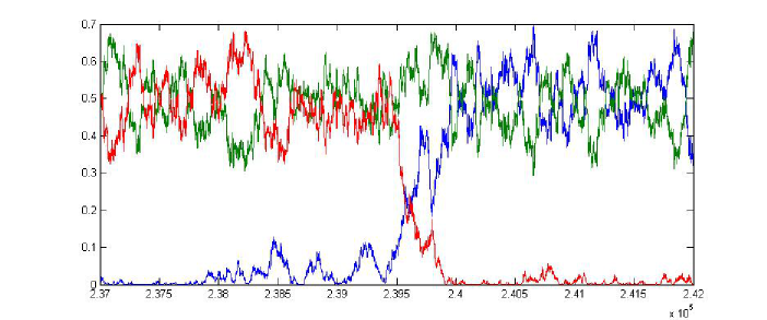
An example of system trajectory is presented in Figure 1 with a zoom of one of transitions between the metastable states shown in Figure 2.
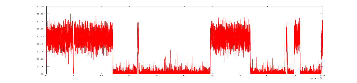
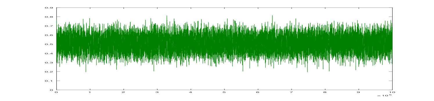
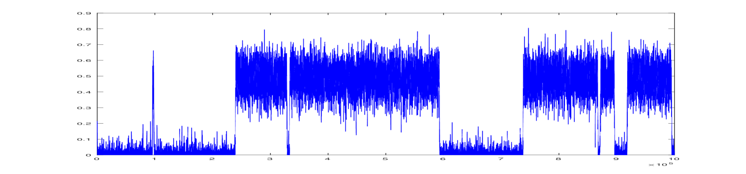
The associated potential function has two global maxima at and , corresponding to the two maximum cliques. In game theoretic terminology, these are two evolutionarily stable strategies. In this simple example, two maximal, and also maximum, cliques are just the two edges.
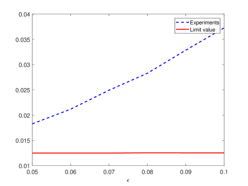
At the maxima, the potential achieves the value of 3/8. It is easy to see from the symmetry of the problem and one-dimensional optimization that the easiest path to reach one maximum from the other goes through the point with the value of the potential 7/20. Thus, in formula (21) we have that
In Figure 3 we plot vs , where is the average exit time obtained from experiments and changes from 0.1 down to 0.05. We note that for values of smaller than 0.05, the exit times become excessively large and we cannot collect enough reliable statistics. Figure 3 suggests that formula (21) describes correctly the asymptotics of the system for small values of .
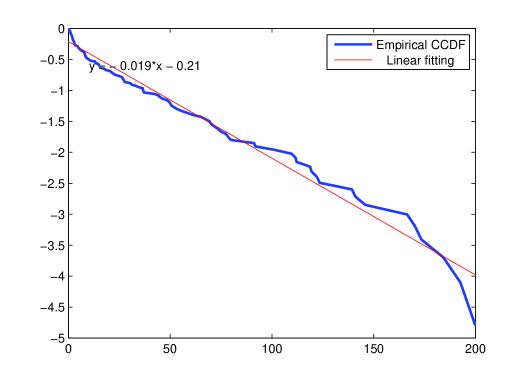
We also plot in Figure 4 the empirical complementary cumulative distribution function of the exit times for in semi-log scale. An approximately linear shape of the curve is in agreement with our expectation that the exit times are exponentially distributed. In all numerical experiments of this section we took the step size and the number of steps between one and ten million depending on the value of .
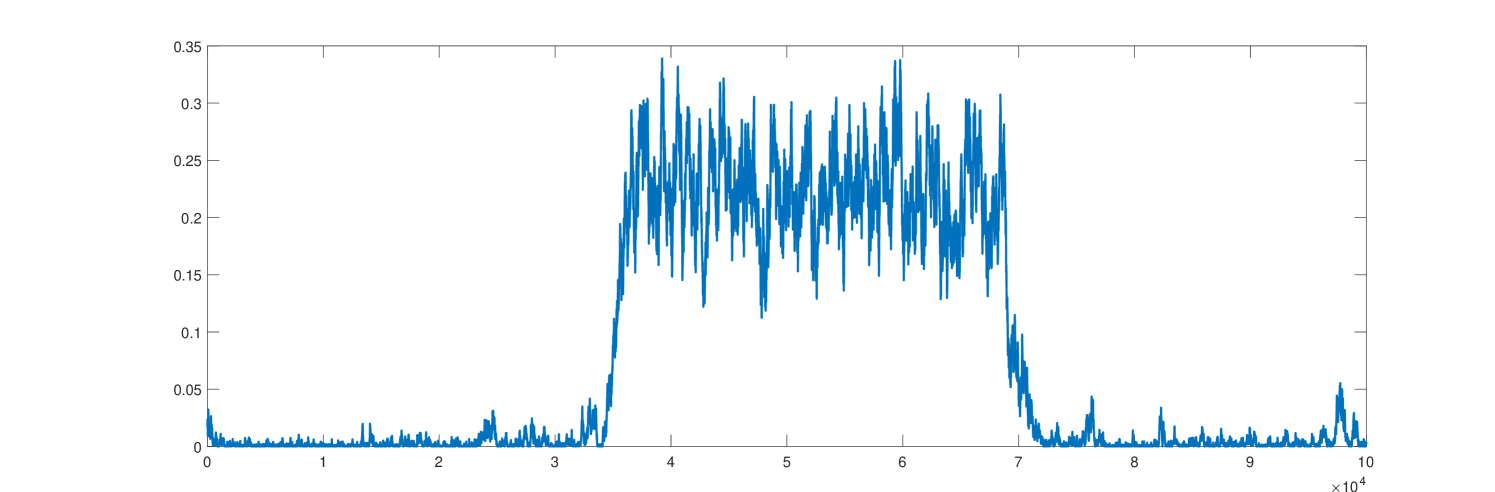
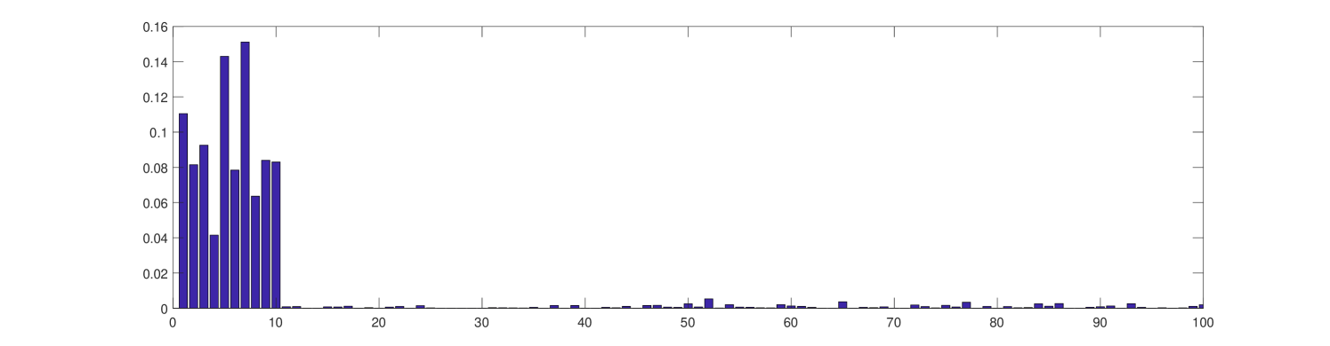
Our second numerical example is based on a sample of Erdős-Rényi random graph with vertices, with the edge probability , and with the noise level in the stochastic replicator dynamics. According to [9, Chapter 11], with high probability, the size of the maximum clique in Erdős-Rényi graph is either or . The substitution of , into the latter formulas indicates that in our example the maximum clique size is either 6 or 7. Furthermore, using [9, Eq. (11.6)], we calculate that the expected number of maximal cliques is 1273 in . The cliques of sizes 3 and 4 contribute most to this number. Thus, it is no surprise that most often we observe the cliques of sizes 3 and 4 and rarely 5. In our experiments, we could never observe a clique of size 6 or 7. The system moves from one metastable state to another and it can take a very long time for the system to come across the metastable state corresponding to the maximum clique. A sample of the intermittent evolution of one subpopulation fraction is shown in Figure 5.
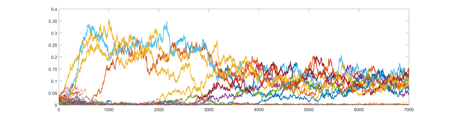
Next, we planted a clique of size 10 in the same realization of . We have chosen the size 10, because is believed to be the critical scaling for detecting the planted clique [4, 40]. It is interesting to observe that in most simulation runs the system state is concentrated on the subpopulations corresponding to the planted clique (see as example Figures 6 and 7).
The planted clique experiments, in agreement with the theoretical results from [4, 40], indicate that there is a critical threshold such that, if cardinality of a tightly interacting subpopulation (clique) exceeds this threshold, the system will fairly quickly converge to the metastable state corresponding to the planted clique and will remain in that metastable state over long time intervals.
6 Conclusions and future research
We studied the phenomena of metastability and quasi-invariance as well as intermittent dynamics of a class of stochastic replicator equation in the small noise regime by invoking the Freidlin-Wentzell theory for small noise asymptotics of diffusions and some recent works on quasi-stationarity. We further specialized these results to a noisy replicator dynamics on graphs, with numerical experiments that confirmed our theoretical observations. We see a number of interesting future research directions worth note.
-
1.
The exit time from the domain of attraction of a stable equilibrium is approximately exponentially distributed. Our example of a stochastic replicator dynamics on graphs shows that an exponential distribution still remains a very good approximation even for the empirical distribution of exit times when the identity of the metastable state is erased, so that each exit episode could be from a different metastable state. In some highly irregular potential functions, however, the exit distribution is observed to be closer to Pareto [23]. This could be because of clusters of closely spaced metastable states at many length scales, which leads to aggregate effects from a large number of individually exponential random variables. Clearly a more refined analysis is needed to explain this observation.
-
2.
In the context of graph problems, estimating the depth of the deepest well of the potential and finding the precise scaling behavior of the mixing time with the size of the graph (see, e.g., [52]) are interesting problems, as is that of characterizing the mixing time in terms of other related stopping times such as hitting times [46]. Specializing further the graph dynamics to the planted clique problem [4, 40], it would be interesting to explore for what scales and after what time the clique becomes detectable by the replicator dynamics. These questions have been investigated for a different Metropolis dynamics in [40]. It will be interesting to carry out a parallel development for our model emphasizing the role of metastability.
Acknowledgements
This work was partly supported by EU Project Congas FP7-ICT-2011-8-317672, CEFIPRA Grants 5100-IT and IFC/DST-Inria-2016-01/448 and ARC Discovery Grant DP 160101236. We thank the referees and the editor for their careful reading and valuable suggestions which have immensely improved this article. We would like to acknowledge the fruitful discussions with Henrik Jensen and Jelena Grujić. We also thank Professors Siva Athreya, K. Suresh Kumar, Laurent Miclo, Kavita Ramanan, K. S. Mallikarjuna Rao and Alexander Veretennikov for valuable pointers to the literature.
This is the author version of the paper accepted to Dynamic Games and Applications journal.
References
- [1] Absil, P.-A., Mahoney, R. and Sepulchre, R. (2008) Optimization Algorithms on Matrix Manifolds, Princeton Uni. Press, Princeton, NJ.
- [2] Aiba, K. (2015) “Waiting times in evolutionary dynamics with time-decreasing noise”, International J. Game Theory 44(2), 499-514.
- [3] Akin, E. (1979) The Geometry of Population Genetics, Springer Verlag, Berlin.
- [4] Alon, N., Krivelevich, M. and Sudakov, B. (1998) “Finding a large hidden clique in a random graph”, Random Structures and Algorithms 13(3-4), 457-466.
- [5] Anderson, R. F. and Orey, S. (1976) “Small random perturbation of dynamical systems with reflecting boundary”, Nagoya Math. J. 60, 189-216.
- [6] Avrachenkov, K., Borkar, V. S. and Nemirovski, D. (2010) “Quasi-stationary distributions as centrality measures for the giant strongly connected component of a reducible graph”, J. Computational and Appl. Math. 234(11), 3075-3090.
- [7] Bass, R. F. and Perkins, E. A. (2002) “Degenerate stochastic differential equations with Hölder continuous coefficients and super-Markov chains”, Trans. of the American Math. Society 355(1), 373-405.
- [8] Bianchi, A. and Gaudilliere, A. (2016) “Metastable states, quasi-stationary and soft measures”, Stochastic Processes and Their Applications 126(6), 1622-1680.
- [9] Bollobas B. (2001) Random Graphs, 2nd ed., Cambridge University Press.
- [10] Bomze, I. M. (1997) “Evolution towards the maximum clique”, J. Global Optimization 10(2), 143-164.
- [11] Bomze, I. M., Budinich, M., Pardalos, P. M. and Pelillo, M. (1999) “The maximum clique problem”. In Handbook of Combinatorial Optimization (pp. 1-74). Springer.
- [12] Bomze, I. M., Budinich, M., Pelillo, M. and Rossi, C. (2002) “Annealed replication: a new heuristic for the maximum clique problem”, Discrete Applied Mathematics, 121(1), 27-49.
- [13] Bomze, I. M., Locatelli, M. and Tardella, F. (2008) “New and old bounds for standard quadratic optimization: dominance, equivalence and incomparability”, Mathematical Programming (Ser. A), 115(1), 31-64.
- [14] Börgers, T. and Sarin, R. (1997) “Learning through reinforcement and replicator dynamics”, Journal of Economic Theory 77(1), 1-14.
- [15] Borkar, V. S. (2008) Stochastic Approximation: A Dynamical Systems Viewpoint, Hindustan Publ. Agency, New Delhi, and Cambridge Uni. Press, Cambridge, UK.
- [16] Borkar, V.S. and Sundaresan R. (2012) “Asymptotics of the invariant measure in mean field model with jumps”, Stochastic Systems, 2, 322-380.
- [17] Borkar, V. S. and Kumar, K. S. (2010) “A new Markov selection procedure for degenerate diffusions”, Journal of Theoretical Probability 23(3), 729-747.
- [18] Bovier, A. and Den Hollander, F. (2015) Metastability: A Potential Theoretic Approach, Springer Verlag, Berlin-Heidelberg.
- [19] Cabrales, A. (2000). Stochastic replicator dynamics. International Economic Review, 41(2), 451-481.
- [20] Catoni, O. (1991) “Sharp large deviations estimates for simulated annealing algorithms.” Annales de l’IHP Probabilités et statistiques. Vol. 27. No. 3.
- [21] Catoni, O. (1992) “Rough large deviation estimates for simulated annealing: Application to exponential schedules.” Annals of Probability, 20(3), 1109-1146.
- [22] Champagnat, N. and Villemonais, D. (2016) “Exponential convergence to quasi-stationary distribution and Q-process”, Prob. Theory and Related Fields 164(1), 243-283.
- [23] Christensen, K., Di Collobiano, S. A., Hall, M. and Jensen, H. J. (2002) “Tangled nature: A model of evolutionary ecology”, Journal of Theoretical Biology 216(1), 73-84.
- [24] Collet, P., Martinez, S. and San Martin J. (2014) Quasi-stationary Distributions: Markov Chains, Diffusions and Dynamical Systems, Springer Verlag, Berlin-Heidelberg.
- [25] Corradi, V. and Sarin, R. (2000) “Continuous approximations of stochastic evolutionary game dynamics”, J. Economic Theory 94(2), 163-191. (Corrigendum in ibid., 140(1) (2008), e2-e4.)
- [26] Eckmann, J. P. and Ruelle, D. (1985) “Ergodic theory of chaos and strange attractors”, Reviews of Modern Physics 57(3), 617-656.
- [27] Foster, D. and Young H. P. (1990) “Stochastic evolutionary game dynamics”, Theoretical Population Biology 38(2), 219-232. (Correction note in ibid. (1997) 51(1), 77-78.)
- [28] Freidlin, M. I. and Wentzell, A. D. (2012) Random Perturbations of Dynamical Systems (3rd ed.). Springer Verlag, New York.
- [29] Fudenberg, D. and Harris, C. (1992) “Evolutionary dynamics with aggregate shocks”, J. Economic Theory 57(2), 420-441.
- [30] Fudenberg, D. and Levine, D. K. (1998) Theory of Learning in Games, MIT Press, Cambridge, Mass.
- [31] Fudenberg, D. and Tirole, J. (1991) Game Theory, MIT Press, Cambridge, Mass.
- [32] Gao, X., Zhong, W. and Mei, S. (2013) “Stochastic evolutionary game dynamics and their selection mechanisms”, Computational Economics 41(2), 233-247.
- [33] Hajek, B. (1988) “Cooling schedules for optimal annealing”, Mathematics of Operations Research 13(2), 311-329.
- [34] Harsanyi, J. C. and Selten, R. (1988) A General Theory of Equilibrium Selection in Games, MIT Press, Cambridge, Mass.
- [35] Hofbauer, J. and Imhof, L. A. (2009) “Time averages, recurrence and transience in stochastic replicator dynamics”, Annals Appl. Prob. 19(4), 1347-1368.
- [36] Hofbauer, J. and Sigmund, K. (1998) Evolutionary Games and Population Dynamics, Cambridge Uni. Press, Cambridge, UK.
- [37] Hsu, E. P. (2002) Stochastic Analysis on Manifolds, Graduate Studies in Mathematics Vol. 38, American Math. Society.
- [38] Ikeda, N. and Watanabe, S. (1989) Stochastic Differential Equations and Diffusion Processes (2nd edition), North Holland–Kodansha, Amsterdam/Tokyo.
- [39] Imhof, L. A. (2005) “The long-run behavior of the stochastic replicator dynamics”, Annals Appl. Prob., 15(1B), 1019-1045.
- [40] Jerrum, M. (1992). “Large cliques elude the Metropolis process”, Random Structures and Algorithms 3(4), 347-359.
- [41] Kang, W. and Ramanan, K. (2014) “Characterization of stationary distributions of reflected diffusions”, Ann. Applied Prob. 24(4), 1329-1374.
- [42] Khasminskii, R. and Potsepun, N. (2006) “On the replicator dynamics behavior under Stratonovich type random perturbations”, Stochastics and Dynamics 6(2), 197-211.
- [43] Kramers, H. A. (1940) “Brownian motion in a field of force and the difffusion model of chemical reactions”, Physica 7, 284-304.
- [44] Krylov, N. V. (1973) “The selection of a Markov proccess from a Markov system of processes” (in Russian) Izv. Akad. Nauk SSSR, Ser. Mat. 37, 691-708.
- [45] Manapat, M. L., Rand, D. G., Pawlowitsch, C. and Nowak, M. A. (2012) “Stochastic evolutionary dynamics resolve the traveler’s dilemma.”, Journal of Theoretical Biology 303, 119-127.
- [46] Manzo, F. and Scoppola, E. (2016) “Strong times and first hitting”, arXiv preprint arXiv:1606.07244.
- [47] Mäs, M. and Nax, H. H. (2016) “A behavioral study of “noise” in coordination games”, Journal of Economic Theory 162, 195-208.
- [48] Mertikopoulos, P. and Moustakas, A. L. (2010) “The emergence of rational behavior in the presence of stochastic perturbations”, Ann. Appl. Prob. 20(4), 1359-1388.
- [49] Mertikopoulos, P. and Viossat, Y. (2016) “Imitation dynamics with payoff shocks”, Intern. J. Game Theory 45, 291-320.
- [50] Olivieri, E. and Vares, M. E. (2004) Large Deviations and Metastability, Encyclopedia of Mathematics and its Applications Vol. 100, Cambridge Uni. Press, Cambridge, UK.
- [51] Ott, E. (2002) Chaos in Dynamical Systems, Cambridge University Press, Cambridge, UK.
- [52] Panageas I. and Vishnoi N.K. (2016) “Mixing time of Markov chains, dynamical systems and evolution”, in LIPIcs-Leibniz International Proceedings in Informatics (Vol. 55). Schloss Dagstuhl-Leibniz-Zentrum fuer Informatik.
- [53] Pinsky, R. (1985) “On the convergence of diffusion processes conditioned to remain in a bounded region for large time to limiting positive recurrent diffusion processes”, Annals of Probability 13(2), 363-378.
- [54] Piovani, D., Grujić, J. and Jensen, H. J. (2016) “Linear stability theory as an early warning sign for transitions in high dimensional complex systems”, Journal of Physics A: Mathematical and Theoretical 49(29), 295102.
- [55] Sandholm, W. H. (2011) Population Games and Evolutionary Dynamics, MIT Press, Cambridge, Mass.
- [56] Sandholm, W. H., Documaci, E. and Lahkar, R. (2008) “The projection dynamic and the replicator dynamic”, Games and Economic Behavior 64(2), 666-683.
- [57] Sandholm, W. H. and Staudigl, M. (2016) “Large deviations and stochastic stability in the small noise double limit”, Theoretical Economics 11.1, 279-355.
- [58] Sandholm, W. H. and Staudigl, M., “Sample path large deviations for stochastic evolutionary game dynamics”, ArXiv preprint arXiv:1511.07897.
- [59] Shahshahani, S. (1979) A new mathematical framework for the study of linkage and selection, Mem. American Math. Society 211.
- [60] Tanaka, H. (1979) “Stochastic differential equations with reflecting boundary condition in convex regions”, Hiroshima Math. J. 9, 163-177.
- [61] Taylor, P. D. and Jonker, L. B. (1978) “Evolutionary stable strategies and game dynamics”, Mathematical Biosciences 40(1+2), 145-156.
- [62] Tokita, K. and Yasutomi, A. (2003) “Emergence of a complex and stable network in a model ecosystem with extinction and mutation”, Theoretical Population Biology 63(2), 131-146.
- [63] Turelli, M. (1977) “Random environments and stochastic calculus”, Theoretical Population Biology 12(2), 140-178.
- [64] van Damme, E. (2002) Stability and Perfection of Nash Equilibria (2nd ed.), Springer Verlag, Berlin-Heidelberg.
- [65] Weibull, J. (1995) Evolutionary Game Theory, MIT Press, Cambridge, Mass.
- [66] Watanabe, S. and Yamada, T. (1971) “On the uniqueness of solutions of stochastic differential equations II”, Journal of Mathematics of Kyoto University 11(3), 553-563.
- [67] Young, H. P. (1998) Individual Strategy and Social Structure, Princeton Uni. Press, Princeton, NJ.