Metric thickenings, Borsuk–Ulam theorems, and orbitopes

The classical Borsuk–Ulam theorem states that any continuous map $f\colon S^{n}\to\mathbb{R}^{n}$ identifies some point with its antipode: $f(x)=f(-x)$ for some $x\in S^{n}$. Equivalently, any odd map $f\colon S^{n}\to\mathbb{R}^{n}$, namely a map satisfying $f(-x)=-f(x)$ for all $x\in S^{n}$, must have a zero: $f(x)=\vec{0}$ for some $x\in S^{n}$. For lower-dimensional codomains, Gromov’s “waist of the sphere” theorem gives quantitative bounds for size of the preimage of some point: for any map $f\colon S^{n}\to\mathbb{R}^{k}$ with $k\leq n$, there is a point $y\in\mathbb{R}^{k}$ such that $\varepsilon$-neighborhoods of $f^{-1}(y)$ have volume bounded below by the volume of the $\varepsilon$-neighborhood of an $(n-k)$-dimensional equator of $S^{n}$ [22, 23, 35]. Here we investigate quantified generalizations of the Borsuk–Ulam theorem for maps to Euclidean space of dimension greater than $n$; see [33] for a different generalization. While a generic odd map $f\colon S^{n}\to\mathbb{R}^{k}$ for $k>n$ does not have a zero, we will show that a convex combination of function values must achieve zero for points contained in a set of diameter strictly less than $\pi$. Further, the diameter bounds obtained are sharp for maps of the form $S^{1}\to\mathbb{R}^{k}$, $S^{n}\to\mathbb{R}^{n+1}$, and $S^{n}\to\mathbb{R}^{n+2}$.

In the following, $r_{n}$ denotes the diameter of a regular $(n+1)$-simplex inscribed into $S^{n}$, where $S^{n}$ carries the standard spherical metric and where each great circle has length $2\pi$.

This result generalizes, with the same diameter bound, to odd maps $f\colon S^{2n-1}\to\mathbb{R}^{2kn+2n-1}$. When $k=0$, we recover the classic Borsuk–Ulam theorem.

We remark that the diameter bound obtained in Theorem 2 also applies to odd and continuous maps $f\colon S^{2n}\to\mathbb{R}^{2kn+2n-1}$; indeed, $f$ restricted to the equator $S^{2n-1}\hookrightarrow S^{2n}$ is odd and continuous with the same codomain.

The diameter bounds in Theorems 1 and 3 are optimal. In the case of the circle, there exist odd maps $f\colon S^{1}\to\mathbb{R}^{2k}\subseteq\mathbb{R}^{2k+1}$ already into one dimension lower such that $\mathrm{conv}(f(X))$ misses the origin for any set $X$ of diameter less than $\frac{2\pi k}{2k+1}$. Constructing such an example map $f$ also proves a result about the structure of zeros of raked trigonometric polynomials, which we explain next.

A trigonometric polynomial is an expression of the form $p(t)=c+\sum_{k=1}^{n}a_{k}\cos(kt)+b_{k}\sin(kt)$, inducing a map $S^{1}\to\mathbb{R}$. In the case that $c=0,$ we call $p$ a homogeneous trigonometric polynomial. The set $S\subseteq\{1,\dots,n\}$ of integers $k$ with $a_{k}\neq 0$ or $b_{k}\neq 0$ is called the spectrum of $p$, and the largest integer in $S$ is the degree of $p$. The spectrum of $p$ constrains the set of roots of $p$; for example, if $p$ is homogeneous of degree $n$ then it has a root on any closed circular arc of length $\frac{2\pi n}{n+1}$; see [9, 20]. Kozma and Oravecz in [29] give upper bounds on the length of an arc where a trigonometric polynomial with spectrum bounded away from zero (that is, $S\subseteq[k,n]$) is non-zero. If the spectrum of $p$ consists only of odd integers, then $p$ is called a raked trigonometric polynomial. We show the following structural result about the roots of raked trigonometric polynomials:

The proof of the first part of Theorem 4 can be used to imply that the quantitative bound on the diameter in Theorem 1 is tight, while the second part of this theorem is a corollary of Theorem 1.

The relation between Theorems 1 and 4 is explained by choosing $f\colon S^{1}\to\mathbb{R}^{2k}\subseteq\mathbb{R}^{2k+1}$ to be the symmetric moment curve

which is an odd function. The convex hull of the curve $\mathrm{SM}_{2k}$ is referred to as the Barvinok–Novik orbitope $\mathcal{B}_{2k}$. Now, Theorem 1 implies that there is a set $X\subseteq S^{1}$ of diameter $\frac{2\pi k}{2k+1}$ such that $\mathrm{conv}(\mathrm{SM}_{2k}(X))$ captures the origin. Thus, for any given $z\in\mathbb{R}^{2k}\setminus\{0\}$, the inner product $\langle z,\mathrm{SM}_{2k}(X)\rangle$ changes sign in $X$ since no hyperplane can separate $\mathrm{SM}(X)$ from the origin. For varying $z$, these inner products range over all possible raked homogeneous trigonometric polynomials, giving the second part of Theorem 4.

The geometry of the Barvinok–Novik orbitope also shows that the bound $\frac{2\pi k}{2k+1}$ in Theorem 1 is optimal:

This also shows that, given $X\subseteq S^{1}$ with $\mathrm{diam}(X)<\frac{2\pi k}{2k+1}$, there is a raked trigonometric polynomial of degree $2k-1$ that is positive on $X$.

For any metric space $X$, we get a continuum spectrum of metric spaces $\mathrm{VR}^{m}(X;r)$, $r>0$, of Vietoris–Rips metric thickenings that capture the local connectivity of $X$ [3]. Note that the superscript $m$ is used here to denote the metric thickening of the Vietoris–Rips complex, as opposed to the geometric realization, and is not a numerical parameter. A point in $\mathrm{VR}^{m}(X;r)$ is a probability measure on $X$ with finite support of diameter at most $r$. Recently, Vietoris–Rips thickenings have been used in topological data analysis and persistent homology [15, 16]; specifically, they allow for a growing filtration of topological spaces associated to a finite collection or sampling of data. Conjecturally, for $X$ the circle $S^{1}$, this spectrum ranges over all odd-dimensional spheres $S^{1},S^{3},S^{5},\dots,$ until eventually becoming contractible.¹¹1These homotopy types are known for the Vietoris–Rips simplicial complexes $\mathrm{VR}(S^{1};r)$ [2], but not yet for the more natural Vietoris–Rips thickenings $\mathrm{VR}^{m}(S^{1};r)$.

As partial evidence towards this conjecture, we explain how Theorem 5 implies that, for scale parameter $r$ in this range, the $(2k-1)$-dimensional homology, cohomology, and homotopy groups of $\mathrm{VR}^{m}(S^{1};r)$ are nontrivial.

In Section 5, we show that Conjecture 6 is true up to $r=\frac{2\pi}{3}$, the side-length of an inscribed equilateral triangle, where $\mathrm{VR}^{m}(S^{1};r)\simeq S^{3}$. More importantly, we provide a geometric picture of why this homotopy equivalence is plausible for $r\geq 0$, as follows. For $\frac{2\pi(k-1)}{2k-1}\leq r<\frac{2\pi k}{2k+1}$ we define a continuous map $\mathrm{VR}^{m}(S^{1};r)\to\mathbb{R}^{2k}\setminus\{\vec{0}\}$ via the centrally symmetric moment curve $(\cos t,\sin t,\cos 3t,\sin 3t,\ldots)$. We relate $\mathrm{VR}^{m}(S^{1};r)$ to the facial structure of the Barvinok–Novik orbitope by composing with the radial projection map $\mathbb{R}^{2k}\setminus\{\vec{0}\}\to\partial\mathcal{B}_{2k}$. Finally, for $r=\frac{2\pi}{3}$ we obtain the homotopy equivalence $\mathrm{VR}^{m}(S^{1};r)\simeq\partial\mathcal{B}_{4}\cong S^{3}$ via a linear homotopy. This is the only step that we are currently unable to extend to large $r$ and $k$; the missing ingredient is a “diameter non-increasing” property for higher-dimensional Barvinok–Novik orbitopes (Conjecture 22).

To our knowledge, this is the first approach to determine the homotopy type of a Vietoris–Rips thickening by mapping the underlying metric space into a higher-dimensional Euclidean space. This technique is analogous to the “kernel trick” of machine learning, in which data is mapped into a higher dimensional space to illuminate the underlying structure of the data.

As a step towards understanding the relationship between metric thickenings of the circle and the Barvinok–Novik orbitopes, we show that given arbitrary $t_{1},\dots,t_{2k-1}\in S^{1}$, there exists a raked homogeneous trigonometric polynomial $f$ of degree $2k-1$ with a root at each $t_{i}$ and its antipode. Further, the polynomial $f$ alternates signs between these roots, has no other roots in $S^{1}$, and may be written down explicitly in terms of the parameters $t_{1},\dots,t_{2k-1}$ (Theorem 26).

We remark that there is an analogous connection between the Čech thickenings of the circle and the Carathéodory orbitopes, i.e. the convex hull of the curve $(\cos t,\sin t,\cos 2t,\sin 2t,\ldots,\cos kt,\sin kt\bigr{)}$ [38].

A preliminary version of several results in this paper appeared in the second author’s master’s thesis [14].

We say two continuous maps $f,g\colon X\to Y$ are homotopic, written $f\simeq g$, if there exists a continuous map $H\colon X\times[0,1]\to Y$ such that $H(x,0)=f(x)$ and $H(x,1)=g(x)$ for all $x\in X$ [24]. Such a map $H$ is called a homotopy. We say $X$ and $Y$ are homotopy equivalent, denoted $X\simeq Y$, if there exist continuous maps $f\colon X\to Y$ and $g\colon Y\to X$ such that $g\circ f\simeq\mathrm{id}_{X}$ and $f\circ g\simeq\mathrm{id}_{Y}$. We furthermore write $X\cong Y$ if spaces $X$ and $Y$ are homeomorphic.

Given a set of points $S\subseteq X$ in a metric space $(X,d)$, let the diameter of $S$ be $\mathrm{diam}(S)=\sup\{d(x,y)~|~x,y\in S\}$; this value may be infinite.

We equip $S^{1}$ with the geodesic metric (of total circumference $2\pi$), though our results also hold when $S^{1}$ is instead equipped with the restriction of the Euclidean metric on $\mathbb{R}^{2}$. Unless otherwise stated, we will always take a representative $t\in S^{1}=\mathbb{R}/2\pi\mathbb{Z}$ as belonging to $[0,2\pi)$. Let $a,b\in S^{1}$, where $a\neq b$, and where $a$ and $b$ are each identified with a point in $[0,2\pi)$. Define the open arc $(a,b)_{S^{1}}$ as

Define the closed arc $[a,b]_{S^{1}}$ similarly.

We identify an abstract simplicial complex with its geometric realization, which is a topological space.

A point in $\mathrm{VR}(X;r)$ can be written in barycentric coordinates as $\sum_{i=0}^{k}\lambda_{i}x_{i}$, with $\mathrm{diam}(\{x_{0},\ldots,x_{k}\})\leq r$. We emphasize that in this paper we are using the $\leq$ convention instead of the $<$ convention.

While the theorems of [25, 30] describe conditions under which the homotopy type of a manifold is recoverable from a Vietoris–Rips complex for sufficiently small $r\geq 0$, much less is known about the topological behavior of these constructions for large values of $r$, even though large values of $r$ commonly arise in applications of persistent homology [16]. However, more is known in the specific case when the underlying manifold is the circle. The following theorem from [2] is based on [1, 4].

Related papers include [19] which studies the 1-dimensional persistence of Čech and Vietoris–Rips complexes of metric graphs, [46] which extends this to geodesic spaces, [47] which studies approximations of Vietoris–Rips complexes by finite samples even at higher scale parameters, and [49] which applies Bestvina–Brady discrete Morse theory to Vietoris–Rips complexes.

When a metric space $X$ is not finite, it is often impossible²²2A simplicial complex (for example $\mathrm{VR}(X;r)$) is metrizable if and only if it is locally finite [37, Proposition 4.2.16(2)]. to equip $\mathrm{VR}(X;r)$ with a metric without changing the homeomorphism type. In such instances the simplicial complex $\mathrm{VR}(X;r)$ destroys the metric information about the underlying space $X$. This motivates the consideration of the Vietoris–Rips metric thickening, $\mathrm{VR}^{m}(X;r)$, which preserves metric information.

Let $\delta_{x}$ denote the Dirac delta mass at a point $x\in X$.

This metric is also called the Kantorovich, optimal transport, or earth mover’s metric [42, 43, 44]; it provides a notion of distance between probability measures defined on a metric space. Although it exists much more generally [17, 27, 28], the $1$-Wasserstein metric on $\mathrm{VR}^{m}(X;r)$ can be defined as follows. Given $\mu,\mu^{\prime}\in\mathrm{VR}^{m}(X;r)$ with $\mu=\sum_{i=0}^{k}\lambda_{i}\delta_{x_{i}}$ and $\mu^{\prime}=\sum_{j=0}^{k^{\prime}}\lambda_{j}^{\prime}\delta_{x_{j}^{\prime}}$, define a matching $p$ between $\mu$ and $\mu^{\prime}$ to be any collection of non-negative real numbers $\{p_{i,j}\}_{i,j}$ such that $\sum_{j=0}^{k^{\prime}}p_{i,j}=\lambda_{i}$ and $\sum_{i=0}^{k}p_{i,j}=\lambda_{j}^{\prime}$. Define the cost of the matching $p$ to be $\sum_{i,j}p_{i,j}d(x_{i},x_{j}^{\prime})$. The $1$-Wasserstein distance between $\mu,\mu^{\prime}\in\mathrm{VR}^{m}(X;r)$ is then the infimum, varying over all matchings $p$ between $\mu$ and $\mu^{\prime}$, of the cost of $p$.

Note that $\mathrm{VR}^{m}(X;0)$ is isometric to $X$. Contrary to the situation for an arbitrary Vietoris–Rips complex, the embedding $X\to\mathrm{VR}^{m}(X;r)$ into the Vietoris–Rips metric thickening given by $x\mapsto\delta_{x}$ is continuous. In fact, more is true: $\mathrm{VR}^{m}(X;r)$ is an $r$-thickening of $X$ [21, 3]. For this reason, we identify $x\in X$ with the measure $\delta_{x}\in\mathrm{VR}^{m}(X;r)$ in the image of this embedding.

If $M$ is a complete Riemannian manifold with curvature bounded from above and below, then $\mathrm{VR}^{m}(M;r)$ is homotopy equivalent to $M$ for $r$ sufficiently small [3, 6]. This property provides an analogue of Hausmann’s theorem [25] for metric thickenings.

Given a measure $\mu=\sum_{i=0}^{k}\lambda_{i}\delta_{x_{i}}$ with $\lambda_{i}>0$, we denote the support of $\mu$ by $\mathrm{supp}(\mu)=\{x_{0},\ldots,x_{k}\}$.

Convex geometry is the study of convex sets, especially polytopes and their facial structures [50]. Given an arbitrary subset $Y\subseteq\mathbb{R}^{n}$, we let

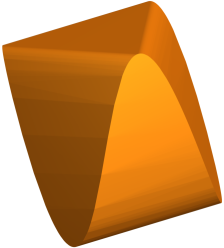
denote the convex hull of $Y$. For example, Figure 1 shows the convex hull of the image of the map $f\colon S^{1}\to\mathbb{R}^{3}$ defined by $f(t)=(\cos(t),\sin(t),\cos(3t))$. Similarly, the conical hull of $Y$ is

Let $Y\subseteq\mathbb{R}^{n}$ be convex. Define a face of $Y$ to be any convex set $F\subseteq Y$ such that, given $x\in F$, if $x=\lambda y+(1-\lambda)z$ for some $0<\lambda<1$ and $y,z\in Y$, then $y,z\in F$.

The centrally symmetric moment curve is analogous to the trigonometric moment curve, with the additional property that it is symmetric under reflecting through the origin.

Here we identify the domain $S^{1}$ with $\mathbb{R}/2\pi\mathbb{Z}$. Since $\mathrm{SM}_{2k}(t+\pi)=-\mathrm{SM}_{2k}(t)$, we say that $\mathrm{SM}_{2k}$ is centrally symmetric about the origin. Interestingly, this curve is closely related to the multidimensional scaling (MDS) embedding $S^{1}\hookrightarrow\mathbb{R}^{2k}$ of the geodesic circle [5, 12, 26, 48]; multidimensional scaling is a way to map a metric space into Euclidean space in a way that distorts the metric (in some sense) as little as possible.

The Barvinok–Novik orbitope is defined by $\mathcal{B}_{2k}=\mathrm{conv}(\mathrm{SM}_{2k}(S^{1}))\subseteq\mathbb{R}^{2k}$ [11]. This convex body is not the convex hull of a finite set of points; it is an orbitope instead of a polytope [38].

The faces of $\mathcal{B}_{2k}$ are known for $k=2$; a subset of these faces are visible in Figure 1 (which is in $\mathbb{R}^{3}$ instead of $\mathbb{R}^{4}$).

Though the facial structure of the Barvinok–Novik orbitopes $\mathcal{B}_{2k}$ is not known for $k>2$, certain neighborliness results have been established [10]. Sinn has shown that the orbitopes are simplicial [39]. Additionally, Vinzant proved that the edges of $\partial\mathcal{B}_{2k}$ consist of all line segments $\mathrm{conv}\left(\mathrm{SM}_{2k}(\{t_{0},t_{1}\})\right)$ with $|t_{0}-t_{1}|\leq\frac{2\pi(k-1)}{2k-1}$ [45]. In other words, the edges of $\mathcal{B}_{2k}$ are the same as the edges of $\mathrm{VR}(S^{1};\frac{2\pi(k-1)}{2k-1})$. The following is an immediate corollary of the work of Sinn and Vinzant.

References

- [1] Michał Adamaszek. Clique complexes and graph powers. Israel Journal of Mathematics, 196(1):295–319, 2013.
- [2] Michał Adamaszek and Henry Adams. The Vietoris–Rips complexes of a circle. Pacific Journal of Mathematics, 290(1):1–40, 2017.
- [3] Michał Adamaszek, Henry Adams, and Florian Frick. Metric reconstruction via optimal transport. SIAM Journal on Applied Algebra and Geometry, 2(4):597–619, 2018.
- [4] Michał Adamaszek, Henry Adams, Florian Frick, Chris Peterson, and Corrine Previte-Johnson. Nerve complexes of circular arcs. Discrete & Computational Geometry, 56(2):251–273, 2016.
- [5] Henry Adams, Mark Blumstein, and Lara Kassab. Multidimensional scaling on metric measure spaces. Accepted to appear in Rocky Mountain Journal of Mathematics, arXiv preprint arXiv:1907.01379, 2019.
- [6] Henry Adams and Joshua Mirth. Vietoris–Rips thickenings of Euclidean submanifolds. Topology and its Applications, 254:69–84, 2019.
- [7] Arseniy Akopyan, Roman Karasev, and Alexey Volovikov. Borsuk–Ulam type theorems for metric spaces. arXiv preprint arXiv:1209.1249, 2012.
- [8] Mark Anthony Armstrong. Basic Topology. Springer Science & Business Media, 2013.
- [9] Alexander G Babenko. An extremal problem for polynomials. Mathematical Notes, 35(3):181–186, 1984.
- [10] Alexander Barvinok, Seung Jin Lee, and Isabella Novik. Neighborliness of the symmetric moment curve. Mathematika, 59(1):223–249, 2013.
- [11] Alexander Barvinok and Isabella Novik. A centrally symmetric version of the cyclic polytope. Discrete & Computational Geometry, 39(1-3):76–99, 2008.
- [12] JM Bibby, JT Kent, and KV Mardia. Multivariate analysis. Academic Press, London, 1979.
- [13] Stephen Boyd and Lieven Vandenberghe. Convex optimization. Cambridge University Press, 2004.
- [14] Johnathan Bush. Vietoris–Rips thickenings of the circle and centrally-symmetric orbitopes. Master’s thesis, Colorado State University, 2018.
- [15] Gunnar Carlsson. Topology and data. Bulletin of the American Mathematical Society, 46(2):255–308, 2009.
- [16] H. Edelsbrunner and J. Harer. Computational Topology: An Introduction. AMS, Providence, 2010.
- [17] David A Edwards. On the Kantorovich–Rubinstein theorem. Expositiones Mathematicae, 29(4):387–398, 2011.
- [18] Jean Gallier and Dianna Xu. Computing exponentials of skew-symmetric matrices and logarithms of orthogonal matrices. International Journal of Robotics and Automation, 18(1):10–20, 2003.
- [19] Ellen Gasparovic, Maria Gommel, Emilie Purvine, Radmila Sazdanovic, Bei Wang, Yusu Wang, and Lori Ziegelmeier. A complete characterization of the one-dimensional intrinsic Čech persistence diagrams for metric graphs. In Research in Computational Topology, pages 33–56. Springer, 2018.
- [20] Anthony D Gilbert and Christopher J Smyth. Zero-mean cosine polynomials which are non-negative for as long as possible. Journal of the London Mathematical Society, 62(2):489–504, 2000.
- [21] Mikhail Gromov. Geometric group theory, volume 2: Asymptotic invariants of infinite groups. London Mathematical Society Lecture Notes, 182:1–295, 1993.
- [22] Mikhail Gromov. Isoperimetry of waists and concentration of maps. Geometric & Functional Analysis GAFA, 13(1):178–215, 2003.
- [23] Larry Guth. The waist inequality in Gromov’s work. The Abel Prize, 2012:181–95, 2008.
- [24] Allen Hatcher. Algebraic Topology. Cambridge University Press, Cambridge, 2002.
- [25] Jean-Claude Hausmann. On the Vietoris–Rips complexes and a cohomology theory for metric spaces. Ann. Math. Studies, 138:175–188, 1995.
- [26] Lara Kassab. Multidimensional scaling: Infinite metric measure spaces. Master’s thesis, Colorado State University, 2019. arXiv preprint arXiv:1904.07763.
- [27] Hans G Kellerer. Duality theorems for marginal problems. Zeitschrift für Wahrscheinlichkeitstheorie und verwandte Gebiete, 67(4):399–432, 1984.
- [28] Hans G Kellerer. Duality theorems and probability metrics. In Proceedings of the Seventh Conference on Probability theory, Braşov, Romania, pages 211–220, 1985.
- [29] Gady Kozma and Ferencz Oravecz. On the gaps between zeros of trigonometric polynomials. Real Analysis Exchange, 28(2):447–454, 2002.
- [30] Janko Latschev. Vietoris–Rips complexes of metric spaces near a closed Riemannian manifold. Archiv der Mathematik, 77(6):522–528, 2001.
- [31] Lásló Lovász. Self-dual polytopes and the chromatic number of distance graphs on the sphere. Acta Scientiarum Mathematicarum, 45(1-4):317–323, 1983.
- [32] Aleksander Maliszewski and Marcin Szyszkowski. Level sets on disks. The American Mathematical Monthly, 121(3):222–228, 2014.
- [33] Andrei V Malyutin and Oleg R Musin. Neighboring mapping points theorem. arXiv preprint arXiv:1812.10895, 2018.
- [34] Jiří Matoušek. Using the Borsuk–Ulam theorem. Springer Science & Business Media, 2008.
- [35] Yashar Memarian. On Gromov’s waist of the sphere theorem. Journal of Topology and Analysis, 3(1):7–36, 2011.
- [36] William H Press, Saul A Teukolsky, William T Vetterling, and Brian P Flannery. Numerical recipes 3rd edition: The art of scientific computing. Cambridge University Press, 2007.
- [37] Katsuro Sakai. Geometric aspects of general topology. Springer, 2013.
- [38] Raman Sanyal, Frank Sottile, and Bernd Sturmfels. Orbitopes. Mathematika, 57(02):275–314, 2011.
- [39] Rainer Sinn. Algebraic boundaries of -orbitopes. Discrete & Computational Geometry, 50(1):219–235, 2013.
- [40] Zeev Smilansky. Convex hulls of generalized moment curves. Israel Journal of Mathematics, 52(1):115–128, 1985.
- [41] Vladimir Mikhailovich Tikhomirov. Some problems in approximation theory. Mathematical notes of the Academy of Sciences of the USSR, 9(5):343–350, 1971.
- [42] Anatoly Moiseevich Vershik. Long history of the Monge–Kantorovich transportation problem. The Mathematical Intelligencer, 35(4):1–9, 2013.
- [43] Cédric Villani. Topics in optimal transportation. Number 58. American Mathematical Soc., 2003.
- [44] Cédric Villani. Optimal transport: Old and new, volume 338. Springer, 2008.
- [45] Cynthia Vinzant. Edges of the Barvinok–Novik orbitope. Discrete & Computational Geometry, 46(3):479–487, 2011.
- [46] Žiga Virk. 1-dimensional intrinsic persistence of geodesic spaces. Topology and Analysis, 2019.
- [47] Žiga Virk. Approximations of 1-dimensional intrinsic persistence of geodesic spaces and their stability. Revista Matemática Complutense, 32:195–213, 2019.
- [48] John Von Neumann and Isaac Jacob Schoenberg. Fourier integrals and metric geometry. Transactions of the American Mathematical Society, 50(2):226–251, 1941.
- [49] Matthew C. B. Zaremsky. Bestvina–Brady discrete Morse theory and Vietoris–Rips complexes. arXiv preprint arXiv:1812.10976, 2018.
- [50] Günter M Ziegler. Lectures on polytopes, volume 152. Springer Science & Business Media, 2012.