\thankstext

e1e-mail: zhao@nucl.sci.hokdai.ac.jp

¹¹institutetext: Nuclear Reaction Data Centre (JCPRG), Hokkaido University, Sapporo 060-0810, Japan ²²institutetext: Department of Physics, Hokkaido University, Sapporo 060-0810, Japan ³³institutetext: Institute of Modern Physics, Fudan University, Shanghai 200433, China ⁴⁴institutetext: Research Center for Nuclear Physics (RCNP), Osaka University, Ibaraki 567-0047, Japan

Microscopic calculations of ⁶He and ⁶Li with real-time evolution method

Q. Zhao\thanksrefe1,addr1 B. Zhou\thanksrefaddr2,addr3 M. Kimura\thanksrefaddr2,addr1,addr4 H. Motoki\thanksrefaddr2 Seung-heon Shin\thanksrefaddr2

Abstract

The low-lying cluster states of ⁶He ( $\alpha$ +n+n) and ⁶Li ( $\alpha$ +n+p) are calculated by the real-time evolution method (REM) which generates basis wave functions for the generator coordinate method (GCM) from the equation of motion of Gaussian wave packets. The $0^{+}$ state of ⁶He as well as the $1^{+}$ , $0^{+}$ and $3^{+}$ states of ⁶Li are calculated as a benchmark. We also calculate the root-mean-square (r.m.s.) radii of the point matter, the point proton, and the point neutron of these states, particularly for the study of the halo characters of these two nuclei. It is shown that REM can be one constructive way for generating effective basis wave functions in GCM calculations.

Keywords:

\alpha

cluster, halo nuclei, r.m.s. radius

1 Introduction

The light nuclei have been studied within the view of the cluster feature for more than five decades Brink1966 ; Fujiwara1980 ; Tohsaki2001 , and various nuclear theories have been developed for the study of nuclear clustering Oertzen2006 ; Horiuchi1991 ; Ito2012 . By assuming the cluster structure, various cluster states of light nuclei have been investigated explicitly Lyu2016 ; Suhara2010 ; Zhou2012 . However, as the number of the constituent clusters and nucleons increases or nuclear system becomes dilute, the number of required basis wave functions increases very quickly. Therefore, a method which can efficiently sift out the basis is highly desired. For this purpose, many efforts have been made, such as the stochastic sampling Suzuki1998 ; Itagaki2003 ; Mitroy2013 and the imaginary-time development method Fukuoka2013 .

Recently, a newly time-dependent many-body theory has been developed in Refs. Imai2019 ; Zhou2020 ; Shin2021 for the calculations of Be and C isotopes. This real-time evolution method (REM) generates the basis wave function using the equation of motion (EOM) which has been applied in the study of heavy-ion collisions Zhang2011 ; Ono1996 ; Ono2019 , but now is found to be very effective in searching the basis wave functions for the microscopic calculations because of its ergodic nature.

We intend to apply the REM on the $0^{+}$ ground state of ⁶He nucleus ( $\alpha$ +n+n). It is a Borromean nucleus consisting of loosely bound and spatially extended three-body systems, typically composed of a compact core plus two weakly bound neutrons (n+n+core) Ogan1999 ; Danilin1998 ; Zhukov1993 . These properties can lead to the huge computational difficulties despite of its simple physical structure. Meanwhile, the low lying states of ⁶Li ( $\alpha$ +n+p) also can be a good comparison, where the more compact states ( $1^{+}$ and $3^{+}$ states with $T=0$ ) and the dilute state ( $0^{+}$ state with $T=1$ ) present simultaneously. In this study, aiming to explore the applicability of REM, we will calculate the $0^{+}$ ground state of ⁶He as well as the low lying states of ⁶Li to reproduce the halo and un-halo properties of these states.

This paper is organized as follows: Section 2 explains the framework of the wave function and the real-time evolution method (REM). The numerical results including the energy and the root-mean-square (r.m.s.) radius are presented and discussed in Sec. 3. The conclusion is summarized in Sec. 4.

2 Framework

2.1 Hamiltonian

We begin with the Hamiltonian given below

\hat{H}=\sum_{i=1}^{A}\hat{t}_{i}-\hat{T}_{c.m.}+\sum_{i<j}^{A}\hat{v}_{N}+\sum_{i<j}^{A}\hat{v}_{C}+\sum_{i<j}^{A}\hat{v}_{LS}

(1)

where $\hat{t}_{i}$ and $\hat{T}_{c.m.}$ denote the kinetic energies of each nucleon and the center of mass, respectively. $\hat{v}_{N}$ denotes the effective nucleon-nucleon interaction and $\hat{v}_{C}$ denotes the Coulomb interaction. $\hat{v}_{LS}$ denotes the spin-orbit interaction.

For the nucleon-nucleon interaction, we take the Volkov No.2 interaction volkov1965 as

\begin{split}V(\mathbf{r})=&(W-M\hat{P}^{\sigma}\hat{P}^{\tau}+B\hat{P}^{\sigma}-H\hat{P}^{\tau})\\ &\times[V_{1}\text{exp}(-r^{2}/c_{1}^{2})+V_{2}\text{exp}(-r^{2}/c_{2}^{2})]~{}.\end{split}

(2)

The corresponding exchange parameters are, $W=0.4$ , $M=0.6$ and $B=H=0.125$ . The parameters in the Gaussian terms are, $V_{1}=-60.65$ MeV, $V_{2}=61.14$ MeV, $c_{1}=1.80$ fm and $c_{2}=1.01$ fm.

We take the G3RS potential Tamagaki1968 ; Yamaguchi1979 as the spin-orbit interaction,

V_{ls}=V_{0}(e^{d_{1}r^{2}}-e^{d_{2}r^{2}})\hat{P}_{31}\hat{L}\cdot\hat{S}~{}.

(3)

The strength parameter $V_{0}$ is set to be 2000 MeV. The Gaussian parameters $d_{1}$ and $d_{2}$ are set to be $5.0$ fm^-2 and $2.778$ fm^-2, respectively.

2.2 Generator coordinate method

In the current work, the single-particle wave function $\phi(\mathbf{r},Z)$ are expressed in a Gaussian form multiplied by the spin-isospin part $\chi_{\tau,\sigma}$ as

\phi(\mathbf{r},Z)=(\frac{2\nu}{\pi})^{3/4}\text{exp}[-\nu(\mathbf{r}-\frac{\bm{z}}{\sqrt{\nu}})^{2}+\frac{1}{2}z^{2}]\chi_{\tau,\sigma}.

(4)

Here the coordinate $Z$ represents the generator coordinates, which includes the three-dimensional coordinate $\bm{z}$ for the spatial part of the wave function as well as the spinor $a$ and $b$ for the spin part $\chi_{\sigma}=a\ket{\uparrow}+b\ket{\downarrow}$ . In this work, the spinor $a$ and $b$ are also regarded as time-dependent variables which will be generated similarly to the spatial coordinates as introduced later. The harmonic oscillator parameter $b=\sqrt{1/(2\nu)}=1.46$ fm, which is same with that used in Refs. Itagaki2003 ; Furumoto2018 .

We describe the ⁶He and ⁶Li as the $\alpha$ -cluster plus two valence nucleon systems in the wave function. Thus the corresponding wave function can be written as

\Phi(Z_{1},Z_{2},\bm{z}_{\alpha})=\mathcal{A}\{\phi(\mathbf{r}_{1},Z_{1})\phi(\mathbf{r}_{2},Z_{2})\Phi_{\alpha}(\mathbf{r}_{3-6},\bm{z}_{\alpha})\}~{}.

(5)

Here $\Phi_{\alpha}$ is the wave function of the $\alpha$ -cluster with $(0s)^{4}$ configuration. $\phi$ are the single-particle wave functions as introduced above, which are used to describe the valence nucleons in ⁶He and ⁶Li. Thus, the coordinates $\mathbf{r}_{1}$ and $\mathbf{r}_{2}$ represent the real spatial position of valence nucleons while $\mathbf{r}_{3-6}$ are for the nucleons in the $\alpha$ -cluster.

Within the framework of generator coordinate method (GCM), the final wave function is the superposition of the basis wave functions with different sets of generator coordinates ( $Z_{1},Z_{2},\bm{z}_{\alpha}$ ):

\Psi=\sum_{i}f_{i}\hat{P}^{J^{\pi}}_{MK}\Phi_{i}(Z_{1,i},Z_{2,i},\bm{z}_{\alpha,i})

(6)

where $\hat{P}^{J^{\pi}}_{MK}$ is the parity and the angular momentum projector. The generator coordinates $\mathbf{Z}$ can be obtained by solving the equation of motion in REM as explained in the next subsection. The corresponding coefficients $f_{i}$ will be determined by the diagonalization of the Hamiltonian.

2.3 Real-time evolution method

In the quantum system, the wave function should satisfy the Schrodinger equation at all times. Thus, the time-dependent variational principle holds for the intrinsic wave function mathematically:

\delta\int dt\frac{\bra{\Phi(\mathbf{Z}_{1},\mathbf{Z}_{2},\mathbf{Z}_{\alpha})}i\hbar~{}d/dt-\hat{H}\ket{\Phi(\mathbf{Z}_{1},\mathbf{Z}_{2},\mathbf{Z}_{\alpha})}}{\langle\Phi(\mathbf{Z}_{1},\mathbf{Z}_{2},\mathbf{Z}_{\alpha})|\Phi(\mathbf{Z}_{1},\mathbf{Z}_{2},\mathbf{Z}_{\alpha})\rangle}=0

(7)

Regarding the coordinate $Z$ as the function of the time $t$ , we obtain the equation of the motion (EOM) as

i\hbar\sum_{j=1,2,\alpha}\sum_{\sigma=x,y,z,a}C_{i\rho j\sigma}\frac{dZ_{j\sigma}}{dt}=\frac{\partial\mathcal{H}_{\text{int}}}{\partial Z^{*}_{i\rho}}

(8)

\mathcal{H}_{\text{int}}\equiv\frac{\bra{\Phi(\mathbf{Z}_{1},\mathbf{Z}_{2},\mathbf{Z}_{\alpha})}\hat{H}\ket{\Phi(\mathbf{Z}_{1},\mathbf{Z}_{2},\mathbf{Z}_{\alpha})}}{\langle\Phi(\mathbf{Z}_{1},\mathbf{Z}_{2},\mathbf{Z}_{\alpha})|\Phi(\mathbf{Z}_{1},\mathbf{Z}_{2},\mathbf{Z}_{\alpha})\rangle}

(9)

C_{i\rho j\sigma}\equiv\frac{\partial^{2}\text{ln}\langle\Phi(\mathbf{Z}_{1},\mathbf{Z}_{2},\mathbf{Z}_{\alpha})|\Phi(\mathbf{Z}_{1},\mathbf{Z}_{2},\mathbf{Z}_{\alpha})\rangle}{\partial Z^{*}_{i\rho}\partial Z_{j\sigma}}

(10)

By following the EOM, from an initial wave function at $t=0$ , the sets of the generator coordinates ( $Z_{1},Z_{2},\bm{z}_{\alpha}$ ) for GCM can be yielded as a function of time $t$ . The ensemble of the basis wave functions $\Phi_{i}(Z_{1,i},Z_{2,i},\bm{z}_{\alpha,i})$ denoted by these sets of the generated coordinates will hold the information of the quantum system. Thus, effective basis can be generated.

In practical calculations, we choose the proper initial excitation energy (the definition can be found in Ref. Imai2019 ; Zhou2020 ) for obtaining various cluster configurations in the evolution. To avoid the clusters or valence nucleons move to unphysical regions, the rebound condition is imposed in our REM calculations. By following the work in Ref. Ono1996 , we add a potential barrier to the Hamiltonian during the REM procedure with the form:

\begin{split}V_{\text{reb}}=\frac{k}{2}\sum_{i}&f(|\mathbf{R}_{i}-\mathbf{R}_{\text{c.m.}}|)\\ f(x)=(x&-d)^{2}\theta(x-d)\\ \mathbf{R}_{i}=\frac{\text{Re}(\bm{z}_{i})}{\sqrt{\nu}},~{}&\mathbf{R}_{\text{c.m.}}=\frac{4}{6}~{}\mathbf{R}_{\alpha}+\frac{1}{6}\sum_{j=1}^{2}\mathbf{R}_{j}~{}.\end{split}

(11)

Here $\mathbf{R}_{i}$ and $\mathbf{R}_{\text{c.m.}}$ represent the spatial position of the $i$ th valence nucleon and the center of mass, respectively, so that $|\mathbf{R}_{i}-\mathbf{R}_{c.m.}|$ is the distance between them. Because of the step function $\theta(x-d)$ , the evolving valence nucleon will face potential barrier when it is $d$ fm far from the center of mass, and be smoothly pushed back in later evolution. We set the strength of the potential barrier $k=6$ MeV/fm², which determines how rapidly the height of the barrier increases. This value is not physically important as long as it is not too large or too small. The rebound radius parameter $d$ is set to be $8$ fm in our calculations, which is large enough for the current work.

We perform the above REM process for the intrinsic wave function of ⁶He and obtain an ensemble of basis. This ensemble of basis are used for both the calculations of ⁶He and ⁶Li.

3 Results

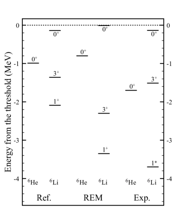
We firstly show the energy spectra for the low-lying states of ⁶He and ⁶Li nuclei in Fig. 1.

Refer to caption — Figure 1: The energy spectra of ⁶He and ⁶Li. Ref. denotes the results from the reference works Itagaki2003 ; Furumoto2018 . REM denotes the results from the current work. Exp. denotes the corresponding experimental data Tilley2004 . The energy is measured relative to the $\alpha$ + n + n threshold, which is set as 0 level with the dotted line. For the calculated results of both in this work and the reference works, the energy of ⁴He is $-27.57$ MeV, while it is $-28.30$ MeV in the experimental data.

Table 1: The numerical results of the

0^{+}

ground state of ⁶He, as well as the

1^{+}

3^{+}

and

0^{+}

states of ⁶Li from the calculations of REM.

	Energy (MeV)	Point matter (fm)	Point proton (fm)	Point neutron (fm)
⁶He ( $0^{+}$ )	-28.37	$2.71$	$2.03$	$2.99$
⁶Li ( $1^{+}$ )	-30.92	$2.65$	$2.66$	$2.65$
⁶Li ( $3^{+}$ )	-29.87	$2.42$	$2.43$	$2.41$
⁶Li ( $0^{+}$ )	-27.58	$2.79$	$2.81$	$2.77$

The experimental data and the corresponding results in the referenced works Itagaki2003 ; Furumoto2018 are also included for comparison. It should be noted that we are using the same Hamiltonian and the same form of the basis wave functions. In Fig. 1, it clearly shows that our REM method provides the almost consistent results for the $0^{+}$ states of ⁶He and ⁶Li nuclei as the references. Besides, for the $1^{+}$ ground state and the $3^{+}$ excited state of ⁶Li, the wave functions from our REM procedure provide better results than the reference work, which means that we have found more sufficient wave function through the evolution with the EOM. These results support the validity of the REM. Furthermore, it should be noted that we are using one ensemble of the basis for both of the ⁶He and ⁶Li calculations, it is interesting that one EOM can reproduce both the $\text{T}=0$ states and $\text{T}=1$ states, and it indicates that the REM may have the potential for the investigation of the isospin mixing states in the future study.

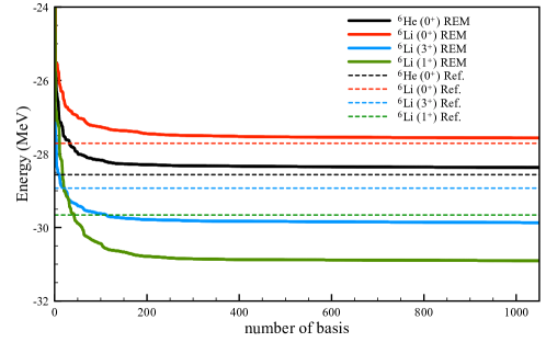
Next we shall check the accuracy of our calculations. We show the energy convergences with the increasing number of basis in Fig. 2. It shows that the huge number of the basis have been included and the binding energies of all these states are well converged. These results prove that the number of basis in our calculations is sufficient to converge the energy results. Furthermore, we can see that the converged results of $1^{+}$ and $3^{+}$ states in our calculation are much lower than the results from the reference works. It denotes that the REM procedure have found more effective basis, which should be included to the total wave function.

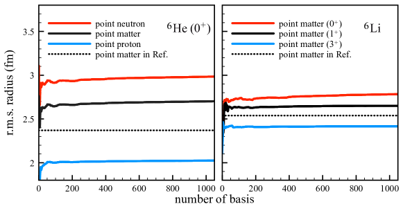
It is also an essential topic to investigate the halo property of the ⁶He nucleus as well as the ⁶Li nucleus. The $0^{+}$ ground state of ⁶He is the well known two-neutron halo. Likewise, the $0^{+}$ excited states of ⁶Li also has the controversial halo property Li2002 . To investigate the halo property in these two nuclei, we calculate the root-mean-square (r.m.s.) radii of ⁶He and ⁶Li with the wave function from REM. The corresponding results are shown in Fig. 3.

In the left panel of this figure, the calculated r.m.s. radii of point matter, point proton and point neutron of the $0^{+}$ state of ⁶He are $2.71$ fm, $2.03$ fm, and $2.99$ fm, respectively. These results are showing the explicit halo property of the ground state of ⁶He. From the right panel of Fig. 3), one can also find that the r.m.s. radius of point matter of the $0^{+}$ state of ⁶Li ( $2.79$ fm) is larger than the radii of its $1^{+}$ ( $2.65$ fm) and $3^{+}$ ( $2.42$ fm). It implies that the $0^{+}$ state of ⁶Li can be treated as a halo state, which is consistent with the experimental conclusion Li2002 . These results show that the halo property of these states can be naturally included in the ensemble of the basis from the REM. Comparing with the reference works, we notice that our results on the r.m.s. radii are larger than the results in the reference works, which are denoted by the dotted lines in Fig. 3. It indicates that our ensemble of basis from REM includes the basis, where valence nucleons spread far from the core, so that we provide more dilute structure for the halo states of ⁶He and ⁶Li nuclei than theirs.

In the end, the detailed numerical results are summarized in Table 1. The current results should be the most accuracy calculation on ⁶He and ⁶Li nuclei within the GCM framework.

4 Conclusion

We perform the calculations for ⁶He and ⁶Li nuclei with a recently developed model named REM, which can generate the ergodic ensemble of the basis wave functions. During this work, we generate the basis wave functions from the procedure of REM and superpose them to construct the total wave functions. The converged results for the energy and the r.m.s. radius of the $0^{+}$ state of ⁶He as well as the $1^{+}$ , $0^{+}$ and $3^{+}$ states of ⁶Li nuclei have been obtained in this work. The halo properties of ⁶He and ⁶Li are well described in the current work, which indicates that the REM can search the basis more efficiently. The current works on ⁶He and ⁶Li nuclei could be the most accurate calculations within the GCM framework to date. The benchmark calculations performed in this work can be instructive for further calculation with REM.

Acknowledgements.

One of the author (M.K.) acknowledges that this work was supported by the JSPS KAKENHI Grant No. 19K03859 and by the COREnet program at RCNP Osaka University.

References

(1) D. M. Brink. in Proceedings of the International School of Physics Enrico Fermi, Course 36, Varenna, edited by C. Bloch, Academic Press, New York, 1966.
(2) Y. Fujiwara, H. Horiuchi, K. Ikeda, M. Kamimura, K. Kato, Y. Suzuki, , and E. Uegaki. Prog. Theor. Phys. Suppl., 68:29, 1980.
(3) A. Tohsaki, H. Horiuchi, P. Schuck, , and G. Roepke. Phys. Rev. Lett., 87:192501, 2001.
(4) T. Kokalova, W. von Oertzen N. Itagaki, , and C. Wheldon. Phys. Rev. Lett., 96:192502, 2006.
(5) H. Horiuchi. Nucl. Phys. A, 522:257, 1991.
(6) M. Ito, N. Itagaki, and K. Ikeda. Phys. Rev. C, 85:014302, 2012.
(7) M. Lyu, Z. Ren, B. Zhou, Y. Funaki, H. Horiuchi, G. Roepke, P. Schuck, A. Tohsaki, C. Xu, and T. Yamada. Phys. Rev. C, 93:054308, 2016.
(8) T. Suhara and Y. Kanada-En’yo. Phys. Rev. C, 82:044301, 2010.
(9) B. Zhou, Y. Funaki, H. Horiuchi, Z. Ren, G. Roepke, P. Schuck, A. Tohsaki, C. Xu, and T. Yamada. Phys. Rev. Lett., 110:262501, 2013.
(10) Y. Suzuki and K. Varga. in Stochastic Variable Approach to Quantum-Mechanical Few-Body Problem, Springer, Berlin, Heidelberg, 1998.
(11) N. Itagaki, A. Kobayakawa, and S. Aoyama. Phys. Rev. C, 68:054302, 2003.
(12) J. Mitroy, S. Bubin, W. Horiuchi, Y. Suzuki, L. Adamowicz, W. Cencek, K. Szalewicz, J. Komasa, D. Blume, and K. Varga. Rev. Mod. Phys., 85:693, 2013.
(13) Y. Fukuoka, S. Shinohara, Y. Funaki, T. Nakatsukasa, and K. Yabana. Phys. Rev. C, 88:014321, 2013.
(14) R. Imai, T. Tada, , and M. Kimura. Phys. Rev. C, 99:064327, 2019.
(15) B. Zhou, M. Kimura, Q. Zhao, and S. Shin. Eur. Phys. J. A, 56:298, 2020.
(16) S. Shin, B. Zhou, and M. Kimura. arXiv:2012.14055, 2020.
(17) G. Q. Zhang, Y. G. Ma, X. G. Cao, C. L. Zhou, X. Z. Cai, D. Q. Fang, W. D. Tian, and H. W. Wang. Phys. Rev. C, 8:034612, 2011.
(18) A. Ono and H. Horiuchi. Phys. Rev. C, 53:845, 1996.
(19) A. Ono. Prog. Part. Nucl. Phys., 105:139, 2019.
(20) Y. Oganessian, V. Zagrebaev, and J. Vaagen. Phys. Rev. Lett., 82:4996, 1999.
(21) B. Danilin, I. Thompson, J. Vaagen, and M. Zhukov. Nucl. Phys. A, 632:383, 1998.
(22) M. Zhukov, B. Danilin, D. Fedorov, J. Bang, I. Thompson, and J. Vaagen. Phys. Rep., 231:151, 1993.
(23) A. Volkov. Nucl. Phys., 7:33, 1965.
(24) R. Tamagaki. Prog. Theor. Phys., 39:91, 1968.
(25) N. Yamaguchi, T. Kasahara, S. Nagata, and Y. Akaishi. Prog. Theor. Phys., 6:1018, 1979.
(26) T. Furumoto, T. Suhara, and N. Itagaki. Phys. Rev. C, 97:044602, 2018.
(27) D.R. Tilley, J.H. Kelley, J.L. Godwin, D.J. Millener, J.E. Purcell, C.G. Sheu, and H.R. Weller. Nucl. Phys. A, 745:155, 2004.
(28) Z. Li, W. Liu, X. Bai, Y. Wang, G. Lian, Z. Li, and S. Zeng. Phys. Lett. B, 527(1):50, 2002.

Microscopic calculations of 6He and 6Li with real-time evolution method