Microwave spectroscopy of Majorana vortex modes

Introduction.  Majorana zero modes were originally proposed within the context of vortices in a topological superconductor (SC) Volovik (1999); Read and Green (2000); Ivanov (2001); Fu and Kane (2008); Sau et al. (2010), and have since emerged as a captivating subject of study in the field of superconductivity. The recent discovery of zero-bias conductance peaks Chen et al. (2018); Wang et al. (2018); Liu et al. (2018); Chen et al. (2019); Machida et al. (2019); Kong et al. (2019); Zhu et al. (2020); Liu et al. (2020); Kong et al. (2021) in the vortex cores of certain Fe-based superconductors Shi et al. (2017); Zhang et al. (2018, 2019a); Peng et al. (2019); Li et al. (2022) has sparked renewed interest in vortex Majorana zero modes (MZMs), which are predicted to be bound in these vortices Sau et al. (2010); Qin et al. (2019); Machida and Hanaguri (2023). The inherent topological nature of vortices as excitations within the superconducting condensate gives hope that the bound states hosted by them would be less susceptible to the disorder, unlike Majorana approaches that require engineered interfaces Banerjee et al. (2023); Aghaee et al. (2023). The key motivation behind studying MZMs is their predicted non-Abelian braiding statistics and possible use in a topologically protected quantum computer Ivanov (2001); Kitaev (2003); Nayak et al. (2008); Grosfeld et al. (2011).

However, the measurement of the topological quantum state of a non-local vortex MZM remains a challenge, hindering progress toward a vortex-based topological qubit. While it is in principle possible to move the vortices and associated MZMs Tewari et al. (2007); Ma et al. (2020, 2021); Hua et al. (2021), it will be challenging to do this adiabatically for a large vortex, but at the same time fast enough to avoid quasiparticle poisoning, the timescale of which in vortices is currently unknown. Alternatively, measurement-based braiding techniques could potentially circumvent the need for moving the MZMs Bonderson et al. (2008). Non-local conductance Liu et al. (2019); Sbierski et al. (2022) and interferometric Fu and Kane (2009); Akhmerov et al. (2009) measurements have been suggested as a means to identify and control Majorana vortex modes. Nevertheless, it is important to note that a microwave-based technique would be optimal for achieving fast readout Smith et al. (2020); Razmadze et al. (2019).

In this paper, we propose a solution to the measurement problem using microwave (MW) techniques, which have been established and demonstrated as an extremely versatile tool to address electronic systems in various experiments Bretheau et al. (2013); van Woerkom et al. (2017); Tosi et al. (2019); Hays et al. (2020, 2021); Fatemi et al. (2022); Matute-Cañadas et al. (2022); Wesdorp et al. (2022). Specifically, we present a microwave-based method for MZM charge parity readout analogous to what has been proposed in different platforms Yavilberg et al. (2015); Ginossar and Grosfeld (2014); Dmytruk et al. (2015); Väyrynen et al. (2015); Yavilberg et al. (2015); Smith et al. (2020).

Our approach focuses on studying the coupling between electrons in the Fe-based superconductor and the microwave photons from a resonator positioned above it. By analyzing the frequency-dependent transmission of the resonator, we can achieve a dispersive readout of the non-local vortex Majorana state. We provide the necessary requirements for the resonator quality factor $Q$ to enable the parity readout. Importantly, our technique can also be applied to vortices in conventional superconductors, offering insights into the lifetime and coherent manipulation of vortex-bound quasiparticles, surpassing the capabilities of existing scanning tunneling microscopy.

General theory of MW coupling to vortex state.  The interaction between the external electromagnetic field with the charge density of the superconductor results in a MW coupling Hamiltonian

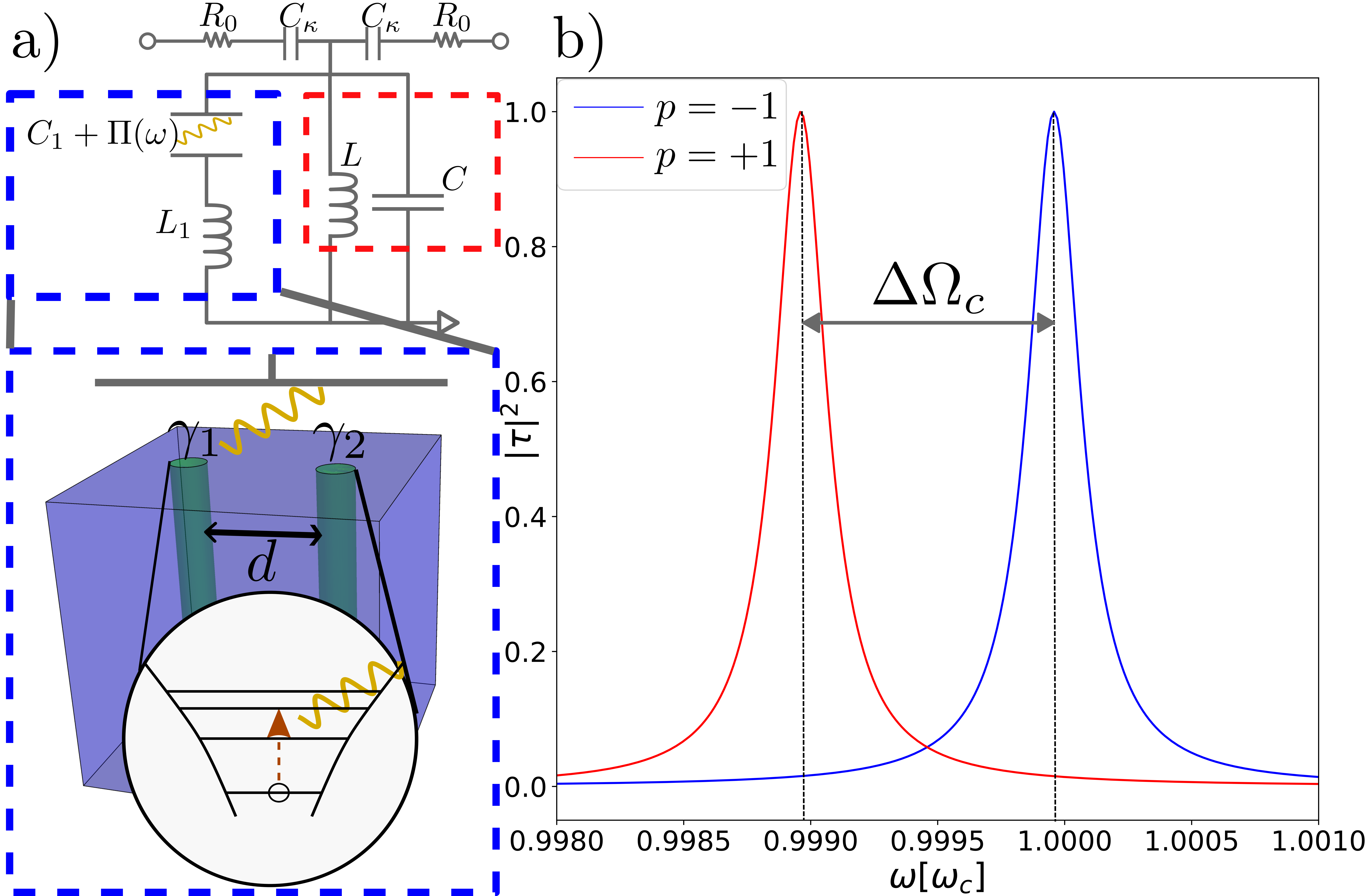
where $\rho_{e}(\mathbf{r})$ is the charge density operator and $V(\mathbf{r})\cos{\omega t}$ is the scalar potential of the external electromagnetic field. This electromagnetic field is created by a resonator, which is within a wavelength of the SC surface. Thus the field can be treated in the quasistatic approximation. The sketch of the measurement setup is shown in Fig. 1(a).

In the static field approximation, screening in the superconductor results in a decay of the field, characterized by a screening length $\lambda_{\text{TF}}$. The scalar potential of the external electromagnetic field can be written as $V(\mathbf{r})=V_{0}e^{-\frac{z}{\lambda_{\text{TF}}}}$, where $z$ is the distance from the top surface of the superconductor and $V_{0}$ is the amplitude of the external field.

In Eq. (1), the charge density $\rho_{e}$ can be expressed as $\rho_{e}=-\frac{1}{2}e\Psi^{\dagger}\tau_{z}\Psi$, where $\Psi=((c_{\uparrow},c_{\downarrow}),(c_{\uparrow}^{\dagger},c_{\downarrow}^{\dagger}))^{T}$ is the Nambu field operator and $\tau_{z}=\text{diag}(1,1,-1,-1)$. In order to expand the field operator in the exact eigenbasis of the unperturbed Hamiltonian $H_{0}$, which is given by Eq. (10) below, we define $\Phi_{n}$ as the spinor wave function of the eigenstate with energy $E_{n}$, and $\Gamma_{n}$ as the second quantized annihilation operators of these quasiparticles.

The eigenstates of the system exhibit a particle-hole symmetry (PHS) that is represented by an antiunitary operator $\mathcal{P}$. For each eigenstate $\Phi_{n}$ with energy $E_{n}$, there exists another eigenstate $\Phi_{-n}=\mathcal{P}\Phi_{n}$ with energy $-E_{n}$. The corresponding annihilation operator satisfies $\Gamma_{-n}=\Gamma_{n}^{\dagger}$. We consider energies below the SC gap and include the excited vortex-bound states (Caroli-de Gennes-Matricon states). The lowest energy state in the system is the Majorana state $\Phi_{\text{M}}$ with energy $E_{\text{M}}$, and its corresponding operator is given by $\Gamma_{\text{M}}=\frac{1}{2}(\gamma_{1}-i\gamma_{2})$, where $\gamma_{1}$ and $\gamma_{2}$ are two Majorana operators as shown in Fig. 1. We aim to read out the occupation number $n_{\text{M}}=\Gamma_{\text{M}}^{\dagger}\Gamma_{\text{M}}$ [or its parity, $(-1)^{n_{\text{M}}}=i\gamma_{1}\gamma_{2}$] of this Majorana zero mode.

Expanding the Nambu spinor $\Psi$ in terms of $\Gamma_{n}$,

the MW coupling (1) can be written as

Here we introduced the matrix elements of the (surface) charge operator $\hat{q}=2\int d^{3}\mathbf{r}\rho_{e}e^{-z/\lambda_{\text{TF}}}$, e.g.,

Because the charge operator preserves PHS, the matrix elements obey the same symmetry, encoded by the relations $q_{n,-m}=-q_{-n,m}^{*}$ and $q_{n.-n}=0$.

Microwave readout of Majorana parity.  In circuit quantum electrodynamics Blais et al. (2021), the MW coupling between a resonator and the superconductor allows us to read out the Majorana parity Dmytruk et al. (2015). The electromagnetic fields induced by the resonator interact with the superconductor in the manner described by the Hamiltonian $\delta H$, Eq. (3). This interaction influences the complex transmission coefficient $\tau^{(p)}(\omega)$ that relates the output and input photonic fields of the resonator. Under the limit $L_{1}C_{1}\ll LC$ (see Fig. 1a) and frequency close to the cavity resonance $\omega_{c}=1/\sqrt{LC_{\text{tot}}}$, we find

where $\kappa=2/(C_{\text{tot}}R^{*})$ is the escape rate of the cavity, and $p=(-1)^{n_{\text{M}}}$ denotes the Majorana parity. We denote $\Pi^{(p)}(\omega)$ the parity-dependent charge-charge correlation function. In the time domain, it is given by $\Pi^{(p)}(t)=-\frac{i}{\hbar}\Theta(t)\langle[\hat{q}(t),\hat{q}(0)]\rangle_{p}$, where $\Theta(t)$ is the Heaviside step function. As shown in Fig. 1a, $C_{\text{tot}}=C+C_{\text{1}}$, where $C$ and $C_{\text{1}}$ are the capacitance of the resonator and the superconductor, respectively. The resonator is coupled with capacitance $C_{\kappa}$ to the input-output transmission line with resistance $R_{0}$, and the effective resistance $R^{*}=\frac{1+\omega_{c}^{2}C^{2}_{\kappa}R_{0}^{2}}{\omega_{c}^{2}C^{2}_{\kappa}R_{0}}$ incorporates the coupling strength $C_{\kappa}$ Göppl et al. (2008).

The interaction between the resonator and the superconductor induces transitions between the Majorana state and the vortex-bound states localized near the top surface. The correlation function $\Pi^{(p)}$ contains information of these transitions and can be written as a sum (from hereon we set $\hbar=1$)

here $\omega_{l}^{(p)}=E_{l}+pE_{\text{M}}$ is the transition frequency and $E_{\text{M}}$, $E_{l}$, $n_{\text{M}}$ and $n_{l}$ are the energies and occupation numbers of the Majorana state and the bound state $l$. The infinitesimal level width $\delta>0$ accounts for causality and $q_{l,\pm\text{M}}$ are the charge matrix elements between bound state $l$ and occupied/unoccupied ($+/-\text{M}$) Majorana state. At low temperatures, in the absence of occupied bound states ($n_{l}=0$), we obtain that $\Pi^{(+)}(\omega)\propto|q_{l,-\text{M}}|^{2}$ for $n_{\text{M}}=0$ and $\Pi^{(-)}(\omega)\propto|q_{l,+\text{M}}|^{2}$ for $n_{\text{M}}=1$. The unequal charge matrix elements $q_{l,\text{M}},q_{l,-\text{M}}$ and transition frequencies $\omega_{l}^{(p)}$ result in different $\Pi^{(\pm)}(\omega)$, which suggests that the MW coupling can be used to probe the Majorana occupation number $n_{\text{M}}$.

The critical cavity Q-factor.  The parity-dependent correlation function $\Pi^{(p)}$ allows for the microwave readout of MZM parity based on the transmission [Eq. (5)]. For simplicity, let us only consider the first vortex-bound state $l=1$ on the surface. Our primary interest lies in the strong coupling regime where the coupling strength $|q_{1,\pm\mathrm{M}}|$ greatly exceeds the level width $\delta$. In this regime, the transmission $|\tau^{(p)}|^{2}$ versus $\omega$ displays two parity-dependent peaks at $\omega>0$. Parity readout is contingent upon the ability to distinguish peaks between different parity, which sets limitations for the cavity Q-factor $Q=\frac{\omega_{c}}{\kappa}$. Here, we define a minimum critical cavity Q-factor $Q_{c}$ required for parity distinction,

where $\Delta\Omega_{c}=\Omega_{c}^{(+)}-\Omega_{c}^{(-)}$ is the peak seperation of two parities in Fig. 1(b), $\Omega_{c}=\frac{1}{2}(\Omega_{c}^{(+)}+\Omega_{c}^{(-)})$ is the average of peak positions, and $\Omega_{c}^{(\pm)}$ are the shifted resonator frequencies of $p=\pm 1$ parity Sup , i.e., $|\tau^{(p)}(\Omega_{c}^{(p)})|^{2}=1$.

The Eq. (7) determines the approximate requirement $Q>Q_{c}$ for distinguishing the different parity resonances. There are two variables that affect the critical cavity Q-factor $Q_{c}$: the parity-dependent charge matrix elements $q_{1,\pm\text{M}}$ and the parity-dependent transition energies $\omega_{1}^{(p)}$ associated with the Majorana energy splitting $E_{\text{M}}$. We define the dimensionless variable $\zeta_{\pm\text{M}}=\sqrt{\frac{U_{\pm\text{M}}}{\omega_{c}}}$ and the capacitive energy $U_{\pm\text{M}}=\frac{q_{1,\pm\text{M}}^{2}}{2C_{\text{tot}}}$.

In the resonant regime, when the resonator frequency is close to the energy of the first bound state, characterized by $|\omega_{c}-E_{1}|\ll\omega_{c}\zeta$, where $\zeta=\frac{1}{2}(\zeta_{+\text{M}}+\zeta_{-\text{M}})$, the transmission curve of each parity exhibits two peaks of width $\kappa$, separated by $2\omega_{c}\zeta$. The parity difference causes a shift in the position of the peaks by $\omega_{c}\delta\zeta-\frac{1}{2}\delta E$, where $\delta\zeta=\zeta_{+\text{M}}-\zeta_{-\text{M}}$ is the dimensionless transition matrix element difference, and $\delta E$ is the change in resonance frequency given by $\delta E=-2E_{\text{M}}$. It is important to note that these two contributions have opposite effects, which can affect the behavior of the transmission curve in this regime. By setting the shift in peak position equal to the escape rate $\kappa$, we obtain

It is worth mentioning that $Q_{c}$ diverges at $\delta\zeta=-E_{\text{M}}/\omega_{c}$ since the peak position does not shift, and thus parity detection becomes difficult.

In the detuning regime, where the resonator frequency is significantly detuned from the first bound state’s energy ($|E_{1}-\omega_{c}|\gg\omega_{c}\zeta,E_{\text{M}}$), the full expression for $Q_{c}$ is more complex compared to the resonant regime (for detailed derivation, see Ref. Sup ). Nevertheless, $Q_{c}$ can be approximated as:

where $|E_{1}-\omega_{c}|\gg\omega_{c}\zeta,E_{\text{M}}$. The two different forms highlight the parity readout based on the parity-dependence of the charge matrix element ($\delta\zeta$) or the transition energy ($E_{\text{M}}$). The first form [Eq. (9a)] depends only on the change in the dimensionless charge matrix element difference $\delta\zeta$ as the parity-dependent factor, while the second form [Eq. (9b)] depends only on the change in transition energy $2E_{\text{M}}$ as the parity-dependent factor.

Model for Fe-based superconductor.  In order to estimate the feasibility of the parity readout discussed above, we will use a microscopic Hamiltonian to evaluate the transition matrix element between the Majorana state and the vortex-bound states.

We will analyze a two-band effective BdG model for an Fe-based superconductor Qin et al. (2019); Zhang et al. (2019b); Ghazaryan et al. (2020); Chiu et al. (2020); Hou and Klinovaja (2021); Barik and Sau (2022). The Hamiltonian in the Nambu basis $\Psi(\textbf{k})=(c_{1\uparrow},c_{1\downarrow},c_{2\uparrow},c_{2\downarrow},c_{1\uparrow}^{\dagger},c_{1\downarrow}^{\dagger},c_{2\uparrow}^{\dagger},c_{2\downarrow}^{\dagger})^{T}$ can be represented as $H_{\text{SC}}=\frac{1}{2}\int dk\Psi^{\dagger}\mathcal{H}_{\text{SC}}\Psi$, where the BdG Hamiltonian $\mathcal{H}_{\text{SC}}$ is given by

here $\mu=5$ meV represents the chemical potential, and $\Delta_{0}=1.8$ meV is the bulk pairing gap. In our lattice model, $H_{0}(\textbf{k})=\nu\eta_{x}(\sigma_{x}\sin k_{x}a+\sigma_{y}\sin k_{y}a+\sigma_{z}\sin k_{z}a)+m(\textbf{k})\eta_{z}$ with $m(\textbf{k})=m_{0}-m_{1}(\cos k_{x}a+\cos k_{y}a)-m_{2}\cos k_{z}a$, where $\eta_{i}$ and $\sigma_{i}$ represent the Pauli matrices that account for the orbital and spin degrees of freedom, respectively Zhang et al. (2019b). In this basis, $\mathcal{P}=\tau_{x}K$, where $\tau_{x}$ represents the Pauli matrix that accounts for the particle-hole degrees of freedom and $K$ denotes complex conjugation. In our numerical simulation, we set $\nu=10$ meV and $a=5$ nm (the lattice constant), $m_{0}=-4\nu,m_{1}=-2\nu$, and $m_{2}=\nu$ so that the system is in the topological phase Zhang et al. (2019b); Hou and Klinovaja (2021) which can have vortex Majorana zero modes.

In the context of our model, we consider the s-wave superconducting pairing potential in the presence of vortices that extend along the z-axis. For a single vortex centered at the origin, the pairing term can be expressed as Blatter et al. (1996)

where $\xi=5$ nm represents the characteristic radius of the vortex and $w=x+iy$.

In our specific model (shown in Fig. 1a), we consider the presence of two vortices, each hosting a pair of MBSs within the Fe-based superconductor. Assuming the vortices are far apart, we can approximate the pairing term as follows,

where $w_{1}$ and $w_{2}$ correspond to the respective locations of the two vortices.

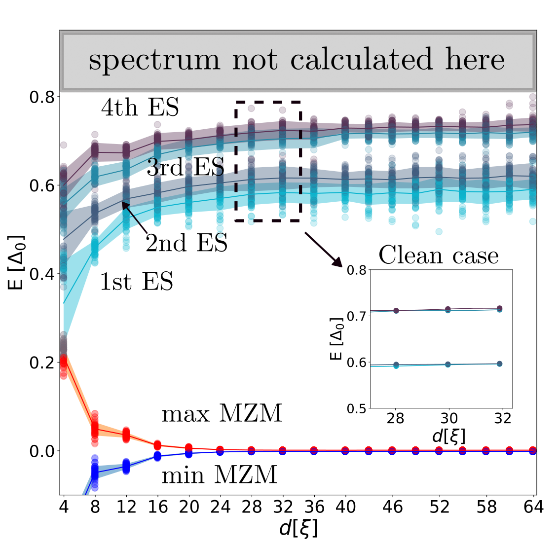
The two-vortex pairing term and the BdG Hamiltonian exhibit a $\text{Z}_{2}$ symmetry represented by $\mathcal{R}_{\text{Z}_{2}}=R(z,\pi)\tau_{z}\eta_{z}$. This operator is characterized by a $\pi$ rotation around the z-axis, with respect to the midpoint of the two vortices, taken here as the origin. Its action on a function $f(x,y,z)$ is given by $R(z,\pi)f(x,y,z)=f(-x,-y,z)$. The symmetry operator has eigenvalues $\pm 1$. The manifestation of this symmetry results in the observation of double degeneracy in the system’s spectrum, as evident in the inset of Fig. 2. The operator $\mathcal{R}_{\text{Z}_{2}}$ commutes with the Hamiltonian (1), establishing a selection rule that governs the allowed MW transitions within the system. According to the selection rule, transitions within the system can only occur between states that share the same eigenvalues of $\mathcal{R}_{\text{Z}_{2}}$. Since the PHS operator $\mathcal{P}=\tau_{x}K$ changes the eigenvalue of $\mathcal{R}_{\text{Z}_{2}}$, at least one of the transition matrix elements $q_{n,+\text{M}},q_{n,-\text{M}}$ vanishes.

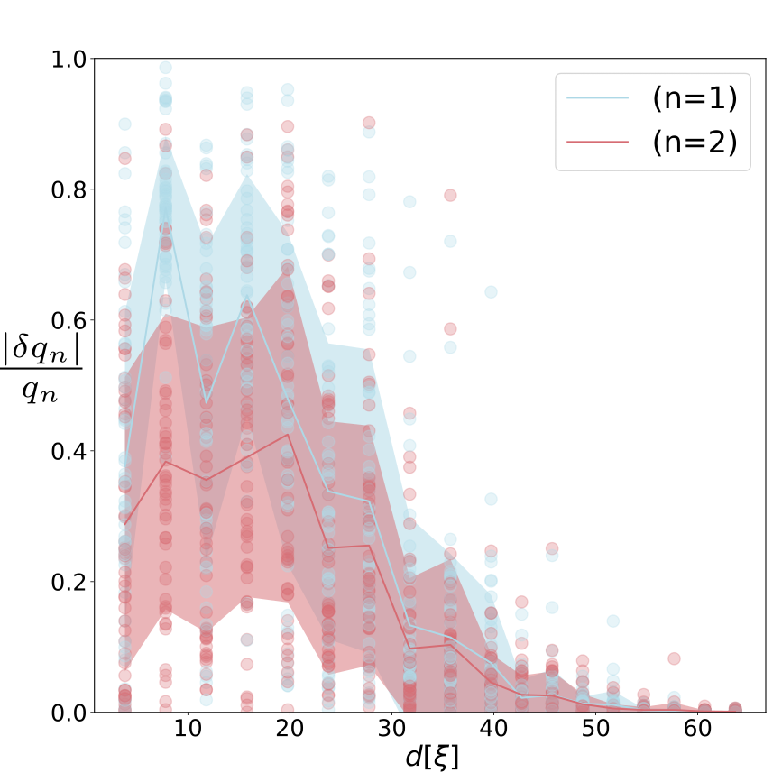
However, the presence of random disorder in realistic conditions disrupts the symmetry, resulting in the elimination of the double degeneracy in the spectrum (Fig. 2). Consequently, this compromises the strict adherence to the selection rule. None of the transition matrix elements $q_{n,+\text{M}},q_{n,-\text{M}}$ are generally zero (Fig. 3). Thus, in realistic experimental settings, the selection rule is not rigorously maintained.

Numerical studies of two-vortex systems.  We employ a numerical approach to investigate a two-vortex system. To perform the numerical analysis, we discretize the Hamiltonian given by Eq. (10) and utilize the Kwant package Groth et al. (2014) in Python to implement and solve the corresponding tight-binding model. The system under consideration is a cuboid with dimensions 500 nm $\crossproduct$ 250 nm $\crossproduct$ 25 nm (refer to Fig. 1a for an illustration), discretized with a lattice constant $a=5$ nm.

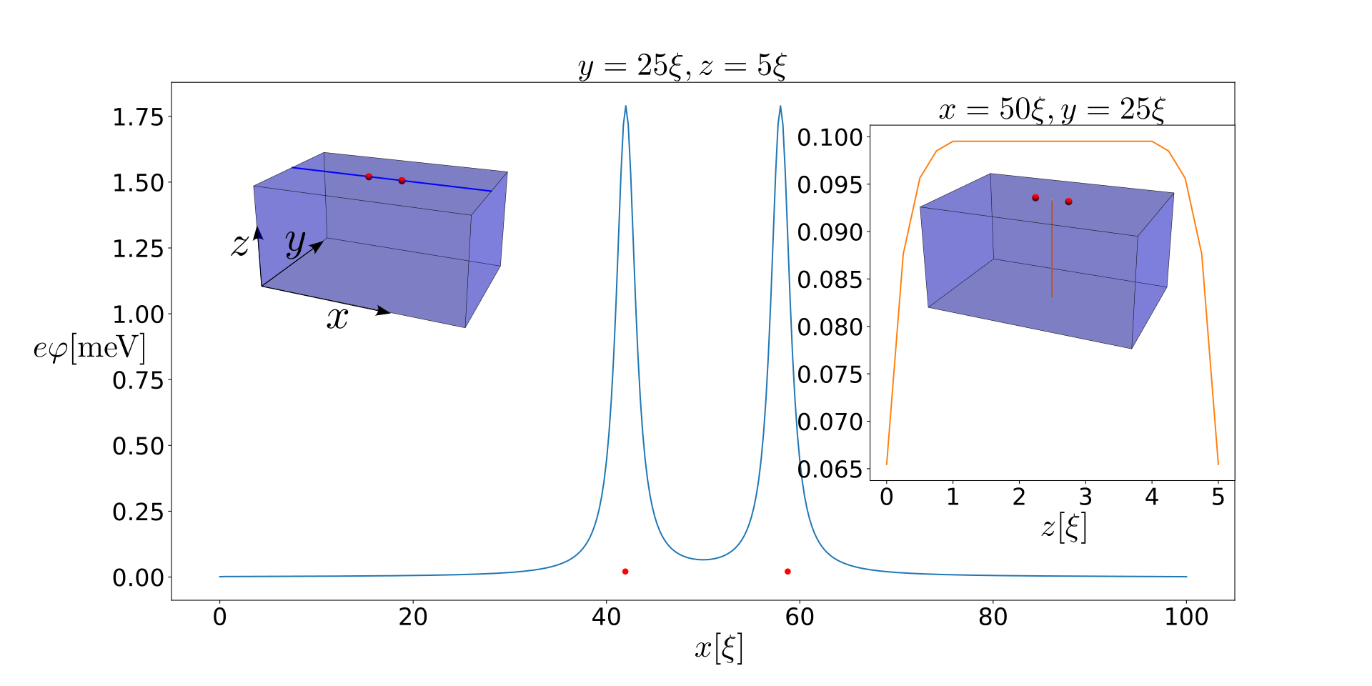
We utilize the results obtained in Ref. Sup to calculate the screened electric potential of two vortices Blatter et al. (1996), which is then included in the real space version of the Hamiltonian in Eq. (10), similar to the way the chemical potential $\mu$ is incorporated. We take the screening length $\lambda_{\text{TF}}$ as one lattice constant. Our investigation encompasses both clean and disordered systems. To model the disorder, we introduce a position-dependent random potential into the Hamiltonian. The disorder potential follows a normal distribution, with the standard deviation of this distribution matching the gap $\Delta_{0}$. The spectrums and charge matrix elements acquired through numerical computations are depicted in Fig. 2 and Fig. 3.

Discussion.  We showed that a microwave coupling enables the parity readout of a non-local Majorana zero mode hosted in a vortex pair. We quantified the sensitivity of the readout by defining a critical cavity Q-factor $Q_{c}$, Eqs. (8)-(9b), required of the resonant cavity coupled to the vortices. To estimate a typical value of $Q_{c}$, let us consider a resonant frequency 5 GHz (much below a typical superconducting gap $\Delta_{0}$) and effective capacitance $1\times 10^{-12}$ F of a typical coplanar waveguide resonator Göppl et al. (2008). In our simulation, we find that the MZM energy $E_{\text{M}}$ for a system with a large vortex separation $d=36\xi$ can be neglected while the first excited state is approximately at $E_{1}\approx 0.58\Delta_{0}\gg\omega_{c}$ (see Fig. 2), implying the system is in the detuning regime. The relevant charge matrix elements are numerically estimated to be $q_{1}\approx 0.009e$ and $\delta q_{1}\approx 0.002e$, the ratio of which is shown in Fig. 3. In this case, Eq. (9a) gives the required critical cavity Q-factor $Q_{c}\sim 10^{8}$, which is close to state-of-the-art experimental conditions Noguchi et al. (2019). Below distance $d\approx 20\xi$, the system is still in the detuning regime of Eq. (9a). There, $Q_{c}\sim 10^{6}$, well within reach of the experiments.

Our method offers a compelling approach to measuring the non-Abelian nature of Majorana zero modes. By employing two resonators to measure quantities $s_{z}=i\gamma_{1}\gamma_{2}$ and $s_{x}=i\gamma_{2}\gamma_{3}$, we can effectively measure two non-commuting parities of MZMs. Through monitoring these observables Vool et al. (2014); Hays et al. (2018), we can estimate quasi-particle poisoning time and MZM hybridization $E_{\text{M}}$. Additionally, incorporating a third resonator to measure $s_{y}=i\gamma_{1}\gamma_{3}$ and an ancillary pair of MZMs, would enable measurement-based braiding Bonderson et al. (2008); Liu et al. (2019); Karzig et al. (2017) within timescales shorter than the quasi-particle poisoning time, when the total parity is conserved. Alternatively, braiding can be achieved through time-dependent control of MZM hybridization in a non-topologically protected manner Trif and Simon (2019). Thus, the resonator-based approach not only allows one to measure the essential quasi-particle poisoning time but also enables one to demonstrate the non-Abelian characteristics of vortex-based MZMs, thus holding significant promise for advancing topological quantum computing and related technologies.

These supplementary materials contain details about the critical cavity Q-factor and screened potential of a vortex.