Mildly Overparameterized ReLU Networks Have a Favorable Loss Landscape
Abstract
We study the loss landscape of both shallow and deep, mildly overparameterized ReLU neural networks on a generic finite input dataset for the squared error loss. We show both by count and volume that most activation patterns correspond to parameter regions with no bad local minima. Furthermore, for one-dimensional input data, we show most activation regions realizable by the network contain a high dimensional set of global minima and no bad local minima. We experimentally confirm these results by finding a phase transition from most regions having full rank Jacobian to many regions having deficient rank depending on the amount of overparameterization.
1 Introduction
The optimization landscape of neural networks has been a topic of enormous interest over the years. A particularly puzzling question is why bad local minima do not seem to be a problem for training. In this context, an important observation is that overparameterization can yield a more benevolent optimization landscapes. While this type of observation can be traced back at least to the works of Poston et al. (1991); Gori & Tesi (1992), it has increasingly become a focus of investigation in recent years. In this article we follow this line of work and describe the optimization landscape of a moderately overparameterized ReLU network with a view on the different activation regions of the parameter space.
Before going into the details of our results we first provide some context. The existence of non-global local minima has been documented in numerous works. This is the case even for networks without hidden units (Sontag & Sussmann, 1989) and single units (Auer et al., 1995). For shallow networks, Fukumizu & Amari (2000) showed how local minima and plateaus can arise from the hierarchical structure of the model for general types of targets, loss functions and activation functions. Other works have also constructed concrete examples of non-global local minima for several architectures (Swirszcz et al., 2017). While these works considered finite datasets, Safran & Shamir (2018) observed that spurious minima are also common for the student-teacher population loss of a two-layer ReLU network with unit output weights. In fact, for ReLU networks Yun et al. (2019b); Goldblum et al. (2020) show that if linear models cannot perfectly fit the data, one can construct local minima that are not global. He et al. (2020) shows the existence of spurious minima for arbitrary piecewise linear (non-linear) activations and arbitrary continuously differentiable loss functions.
A number of works suggest overparameterized networks have a more benevolent optimization landscape than underparameterized ones. For instance, Soudry & Carmon (2016) show for mildly overparameterized networks with leaky ReLUs that for almost every dataset every differentiable local minimum of the squared error training loss is a zero-loss global minimum, provided a certain type of dropout noise is used. In addition, for the case of one hidden layer they show this is the case whenever the number of weights in the first layer matches the number of training samples, . In another work, Safran & Shamir (2016) used a computer aided approach to study the existence of spurious local minima, arriving at the key finding that when the student and teacher networks are equal in width spurious local minima are commonly encountered. However, under only mild overparameterization, no spurious local minima were identified, implying again that overparameterization leads to a more benign loss landscape. In the work of Tian (2017), the student and teacher networks are assumed to be equal in width and it is shown that if the dimension of the data is sufficiently large relative to the width, then the critical points lying outside the span of the ground truth weight vectors of the teacher network form manifolds. Another related line of works studies the connectivity of sublevel sets (Nguyen, 2019) and bounds on the overparameterization that ensures existence of descent paths (Sharifnassab et al., 2020).
The key objects in our investigation will be the rank of the Jacobian of the parametrization map over a finite input dataset, and the combinatorics of the corresponding subdivision of parameter space into pieces where the loss is differentiable. The Jacobian map captures the local dependency of the functions represented over the dataset on their parameters. The notion of connecting parameters and functions is prevalent in old and new studies of neural networks: for instance, in discussions of parameter symmetries (Chen et al., 1993), functional equivalence (Phuong & Lampert, 2020), functional dimension (Grigsby et al., 2022), the question of when a ReLU network is a universal approximator over a finite input dataset (Yun et al., 2019a), as well as in studies involving the neural tangent kernel (Jacot et al., 2018).
We highlight a few works that take a geometric or combinatorial perspective to discuss the optimization landscape. Using dimension counting arguments, Cooper (2021) showed that, under suitable overparameterization and smoothness assumptions, the set of zero-training loss parameters has the expected codimension, equal to the number of training data points. In the case of ReLU networks, Laurent & von Brecht (2018) used the piecewise multilinear structure of the parameterization map to describe the location of the minimizers of the hinge loss. Further, for piecewise linear activation functions Zhou & Liang (2018) partition the parameter space into cones corresponding to different activation patterns of the network to show that, while linear networks have no spurious minima, shallow ReLU networks do. In a similar vein, Liu (2021) study one hidden layer ReLU networks and show for a convex loss that differentiable local minima in an activation region are global minima within the region, as well as providing conditions for the existence of differentiable local minima, saddles and non differentiable local minima. Considering the parameter symmetries, Simsek et al. (2021) show that the level of overparameterization changes the relative number of subspaces that make up the set of global minima. As a result, overparameterization implies a larger set of global minima relative to the set of critical points, and underparameterization the reverse. Wang et al. (2022) studied the optimization landscape in two-layer ReLU networks and showed that all optimal solutions of the non-convex loss can be found via the optimal solutions of a convex program.
1.1 Contributions
For both shallow and deep neural networks we show most linear regions of parameter space have no bad local minima and often contain a high-dimensional space of global minima. We examine the loss landscape for various scalings of the input dimension , hidden dimensions , and number of data points .
-
•
Theorem 5 shows for two-layer networks that if and , then all activation regions, except for a fraction of size at most , have no bad local minima. We establish this by studying the rank of the Jacobian with respect to the parameters. By appealing to results from random matrix theory on binary matrices, we show for most choices of activation patterns that the Jacobian will have full rank. Given this, all local minima within a region will be zero-loss global minima. For generic high-dimensional input data , this implies most non-empty activation regions will have no bad local minima as all activation regions are non-empty for generic data in high dimensions. We extend these results to the deep case in Theorem 14.
-
•
In Theorem 10, we specialize to the case of one-dimensional input data , and consider two-layer networks with a bias term. We show that if , all but at most a fraction of non-empty linear regions in parameter space will have no bad local minima. We remark that this includes the non-differentiable local minima on the boundary between activation regions as per Theorem 13. Further, in contrast to Theorem 5 which looks at all binary matrices of potential activation patterns, in the one-dimensional case we are able to explicitly enumerate the binary matrices which correspond to non-empty activation regions.
-
•
Theorem 12 continues our investigation of one-dimensional input data, this time concerning the existence of global minima within a region. Suppose that the output head has positive weights and negative weights and . We show that if , then all but at most a fraction of non-empty linear regions in parameter space will have global minima. Moreover, the regions with global minima will contain an affine set of global minima of codimension .
-
•
In addition to counting the number of activation regions with bad local minima, Proposition 15 and Theorem 17 provide bounds on the fraction of regions with bad local minima by volume under additional assumptions on the data, notably anti-concentratedness. These results imply that mild overparameterization suffices again to ensure that the ‘size’ of activation regions with bad local minima is small not only as measured by number but also by volume.
1.2 Relation to prior works
As indicated above, several works have studied sets of local and global critical points of two-layer ReLU networks, so it is in order to give a comparison. We take a different approach by identifying the number of regions which have a favorable optimization landscape, and as a result are able to avoid having to make certain assumptions about the dataset or network. Since we are able to exclude pathological regions with many dead neurons, we can formulate our results for ReLU activations rather than LeakyReLU or other smooth activation functions. In contrast to Soudry & Carmon (2016), we do not assume dropout noise on the outputs of the network, and as a result global minima in our setting typically attain zero loss. Unlike Safran & Shamir (2018), we do not assume any particular distribution on our datasets; our results hold for almost all datasets (a set of full Lebesgue measure). Extremely overparameterized networks (with ) are known to follow lazy training (see Chizat et al., 2019); our theorems hold under more realistic assumptions of mild overparameterization or even for high-dimensional inputs. We are able to avoid excessive overparameterization by emphasizing qualitative aspects of the loss landscape, using only the rank of the Jacobian rather than the smallest eigenvalue of the neural tangent kernel, for instance.
2 Preliminaries
Before specializing to specific neural network architectures, we introduce general definitions which encompass all of the models we will study. For any we will write . We will write for a vector of ones, and drop the subscript when the dimension is clear from the context. The Hadamard (entry-wise) product of two matrices and of the same dimension is defined as . The Kronecker product of two vectors and is defined as .
Let denote the set of polynomials in variables with real coefficients. We say that a set is an algebraic set if there exist such that is the zero locus of the polynomials ; that is,
Clearly, and are algebraic, being zero sets of and respectively. A finite union of algebraic subsets is algebraic, as well as an arbitrary intersection of algebraic subsets. In other words, algebraic sets form a topological space. Its topology is known as the Zariski topology. The following lemma is a basic fact of algebraic geometry, and follows from subdividing algebraic sets into submanifolds of .
Lemma 1.
Let be a proper algebraic subset of . Then has Lebesgue measure .
For more details on the above facts, we refer the reader to Harris (2013). Justified by Lemma 1, we say that a property depending on holds for generic if there exists a proper algebraic set such that holds whenever . So if is a property that holds for generic , then in particular it holds for a set of full Lebesgue measure.
We consider input data
and output data
A parameterized model with parameter space is a mapping
We overload notation and also define as a map from to by
Whether we are thinking of as a mapping on individual data points or on datasets will be clear from the context. We define the mean squared error loss by
| (1) |
For a fixed dataset , let denote the set of global minima of the loss ; that is,
If there exists such that , then , so is a global minimum. In such a case,
For a dataset , we say that is a local minimum if there exists an open set containing such that for all . We say that is a bad local minimum if it is a local minimum but not a global minimum.
A key indicator of the local optimization landscape of a neural network is the rank of the Jacobian of the map with respect to the parameters . We will use the following observation.
Lemma 2.
Fix a dataset . Let be a parameterized model and let be a differentiable critical point of the squared error loss equation 1. If , then is a global minimizer.
Proof.
Suppose that is a differentiable critical point of . Then
Since , this implies that . In other words, is a global minimizer. ∎
Finally, in what follows given data we study activation regions in parameter space. Informally, these are sets of parameters which give rise to particular activation patterns of the neurons of a network over the dataset. We will define this notion formally for each setting we study in the subsequent sections.
3 Shallow ReLU networks: counting activation regions with bad local minima
Here we focus on a two-layer network with inputs, one hidden layer of ReLUs, and an output layer. The key takeaway of this section is that moderate overparameterization is sufficient to ensure that bad local minima are scarce. With regard to setup, our parameter space is the input weight matrix in . Our input dataset will be an element and our output dataset an element , where is the cardinality of the dataset. The model is defined by
where is the ReLU activation function applied componentwise. We write , where is the th row of . Since is piecewise linear, for any finite input dataset we may split the parameter space into a finite number of regions on which is linear in (and linear in ). For any binary matrix and input dataset , we define a corresponding activation region in parameter space by
This is a polyhedral cone defined by linear inequalities for each . For each and , we have for all , which is linear in . The Jacobian with respect to is and with respect to is
where denotes the th column of . To show that the Jacobian has rank , we need to ensure that the activation matrix does not have too much linear dependence between its rows. The following result, due to Bourgain et al. (2010), establishes this for most choices of .
Theorem 3.
Let be a matrix whose entries are iid random variables sampled uniformly from . Then is singular with probability at most
The next lemma shows that the specific values of are not relevant to the rank of the Jacobian.
Lemma 4.
Let , for and be vectors, with for all . Then
Using algebraic techniques, we show that for generic , the rank of the Jacobian is determined by . Then by the above results, Lemma 2 concludes that for most activation regions the smooth critical points are global minima (see full details in Appendix A):
Theorem 5.
Let . If
then for generic datasets , the following holds. In all but at most activation regions (i.e., an fraction of all regions), every differentiable critical point of with nonzero entries for is a global minimum.
The takeaway of Theorem 5 is that most activation regions do no contain local minima. However, for a given dataset not all activation regions, each encoded by a binary matrix , may be realizable by the network. Equivalently, is not realizable if and only if and we call such activation regions empty. We therefore turn our attention to evaluating the number of non-empty activation regions. Different activation regions in parameter space are separated by the hyperplanes , , . We say that a set of vectors in a -dimensional space is in general position if any of them are linearly independent, which is a generic property. Standard results on hyperplane arrangements give the following proposition.
Proposition 6 (Number of non-empty regions).
Consider a network with one layer of ReLUs. If the columns of are in general position in a -dimensional linear space, then the number of non-empty activation regions in the parameter space is .
The formula provided above in Proposition 6 is equal to if and only if , and is if . We therefore observe that if is large in relation to and the data is in general position then by Proposition 6 most activation regions are non-empty. Thus we obtain the following corollary of Theorem 5.
Corollary 7.
Under the same assumptions as Theorem 5, if , then for in general position and arbitrary , the following holds. In all but at most an fraction of all non-empty activation regions, every differentiable critical point of with nonzero entries for is a zero loss global minimum.
More generally, for an arbitrary dataset that is not necessarily in general position the regions can be enumerated using a celebrated formula by Zaslavsky (1975), in terms of the intersection poset of the hyperplanes. Moreover, importantly one can show that the maximal number of non-empty regions is attained when the dataset is in general position.
From the above discussion we conclude we have a relatively good understanding of how many activation regions are non-empty. Notably, the number is the same for any dataset that is in general position. However, it is worth reflecting on the fact that the identity of the non-empty regions depends more closely on the specific dataset and is harder to catalogue. For a given dataset the non-empty regions correspond to the vertices of the Minkowski sum of the line segments with end points , for , as can be inferred from results in tropical geometry (see Joswig, 2021).
Proposition 8 (Identity of non-empty regions).
Let . The corresponding activation region is non-empty if and only if is a vertex of for all .
This provides a sense of which activation regions are non-empty, depending on . The explicit list of non-empty regions is known in the literature as the list of maximal covectors of an oriented matroid (see Björner et al., 1999), which can be interpreted as a combinatorial type of the dataset.
4 Shallow univariate ReLU networks: activation regions with global vs local minima
In Section 3 we showed that mild overparameterization suffices to ensure that most activation regions do not contain bad local minima. This result however does not discuss the relative scarcity of activation regions with global versus local minima. To this end in this section we take a closer look at the case of a single input dimension, . Importantly, in the univariate setting we are able to entirely characterize the realizable (non-empty) activation regions.
Consider a two-layer ReLU network with input dimension , hidden dimension , and a dataset consisting of data points. We suppose the network has a bias term . The model is given by
Since we include a bias term here, we define the activation region by
In this one-dimensional case, we first obtain new bounds on the fraction of favorable activation regions to show that most non-empty activation regions have no bad differentiable local minima. We begin with a characterization of which activation regions are non-empty. For , we introduce the step vectors , defined by
Note that and . There are step vectors in total. Intuitively, step vectors describe activation regions because all data points on one side of a threshold value activate the neuron. The following lemma makes this notion precise.
Lemma 9.
Fix a dataset with . Let be a binary matrix. Then is non-empty if and only if the rows of are step vectors. In particular, there are exactly non-empty activation regions.
Using this characterization of the non-empty activation regions, we show that most activation patterns corresponding to these regions yield full-rank Jacobian matrices, and hence the regions have no bad local minima.
Theorem 10.
Let . Suppose that consists of distinct data points, and
Then in all but at most a fraction of non-empty activation regions, is full rank and every differentiable critical point of where has nonzero entries is a global minimum.
Our strategy for proving Theorem 10 hinges on the following observation. For the sake of example, consider the step vectors . This set of vectors forms a basis of , so if each of these vectors was a row of the activation matrix , it would have full rank. This observation generalizes to cases where some of the step vectors are taken to be instead of . If enough step vectors are “collected” by rows of the activation matrix, it will be of full rank. We can interpret this condition in a probabilistic way. Suppose that the rows of are sampled randomly from the set of step vectors. We wish to determine the probability that after samples, enough step vectors have been sampled to cover a certain set. We use the following lemma.
Lemma 11 (Coupon collector’s problem).
Let , and let be positive integers. Let be iid random variables such that for all one has . If
then with probability at least .
This gives us a bound for the probability that a randomly sampled region is of full rank. We finally convert this into a combinatorial statement to obtain Theorem 10. For the details and a complete proof, see Appendix C.
In one-dimensional input space, the existence of global minima within a region requires similar conditions to the region having a full rank Jacobian. Both of them depend on having many different step vectors represented among the rows of the activation matrix. The condition we need to check for the existence of global minima is slightly more stringent, and depends on there being enough step vectors for both the positive and negative entries of .
Theorem 12 (Fraction of regions with global minima).
Let and let have nonzero entries. Suppose that consists of distinct data points,
and
Then in all but at most an fraction of non-empty activation regions , the subset of global minimizers in , , is a non-empty affine set of codimension . Moreover, all global minima of have zero loss.
We provide the proof of this statement in Appendix C. To conclude, for shallow ReLU networks and univariate data we have shown that mild overparameterization suffices to ensure that the loss landscape is favorable in the sense that most activation regions contain a set of global minima of significant codimension and do not contain any local minima. Furthermore, considering both Sections 3 and 4, we have shown in both the one-dimensional and higher-dimensional cases that most activation regions have a full rank Jacobian and contain no bad local minima. This suggests that a large fraction of parameter space by volume should also have a full rank Jacobian. This indeed turns out to be the case and is discussed in Section 6. Finally, we highlight to the reader that we provide a discussion of the function space perspective of this setting in Appendix D.
4.1 Nonsmooth critical points
Our results in this section considered the local minima in the interior of a given activation region. Here we extend our analysis to handle points on the boundaries between regions where the loss is non-differentiable. We consider a network on univariate data as in Section 4. Let be the unit step function:
Here we define the activation regions to include the boundaries:
We assume that the input dataset consists of distinct data points . By the same argument as Lemma 9, an activation region is non-empty if and only if the rows of are step vectors and we derive the following result.
Theorem 13.
Let . If
then in all but at most a fraction of non-empty activation regions , every local minimum of in is a global minimum.
5 Extension to deep networks
While the results presented so far focused on shallow networks, they admit generalizations to deep networks. These generalizations are achieved by considering the Jacobian with respect to parameters of individual layers of the network. In this section, we demonstrate this technique and prove that in deeper networks, most activation regions have no spurious critical points. We consider fully connected deep networks with layers, where layer maps from to , and . The parameter space consists of tuples of matrices
where . We identify the vector space of all such tuples with , where . For , we define the -th layer recursively by
if , and
where is a fixed vector whose entries are nonzero. Then is the final layer output of the network, so the model is given by . We denote the -th row of by . The activation patterns of a deep network are given by tuples
where for each , . For an activation pattern , let denote the subset of parameter space corresponding to . More precisely,
Assuming linear scaling of the second-to-last layer of the network in the number of data points, along with mild restrictions on the other layers, we prove that most activation regions for deep networks have a full rank Jacobian.
Theorem 14.
Let be an input dataset with distinct points. Suppose that for all ,
and that
Then for at least a fraction of all activation patterns , the following holds. For all , has rank .
We provide a proof of this statement in Appendix E.
6 Volumes of activation regions
Our main results so far have concerned the number of activation regions containing bad local versus global minima. Here we compute bounds for the volume of the union of these bad versus good activation regions, which recall are subsets of parameter space. Proofs of all results in this section are provided in Appendix F.
6.1 One-dimensional input data
Consider the setting of Section 4, where we have a network on one-dimensional input data. Recall that for , we defined the activation region by
For , and corresponding step vectors , we also define the individual neuron activation regions by
Let denote the Lebesgue measure. First, we compute an exact formula for the volume of the activation regions intersected with the unit interval. That is, we compute the Lebesgue measure of the set .
Proposition 15.
Let be defined by
Consider data . Then for and ,
Here we define , .
We apply this result to bound the volume of activation regions with full rank Jacobian in terms of the amount of separation between the data points. For overparameterized networks with sufficient separation, the activation regions with full rank Jacobian fill up most of the parameter space by volume.
Proposition 16.
Let . Suppose that the entries of are nonzero. Suppose that for all with , we have and . If
then
6.2 Arbitrary dimension input data
We now consider the setting of Section 3. Our model is defined by
We consider the volume of the set of points such that has rank . We can formulate this problem probabilistically. Suppose that the entries of and are sampled from the standard normal distribution . We wish to compute the probability that the Jacobian has full rank.
Let denote the step function:
For an input dataset , consider the random variable
where , and is defined entrywise. This defines the distribution of activation patterns on the dataset, which we denote by . We say that an input dataset is -anticoncentrated if for all nonzero ,
We can interpret this as a condition on the amount of separation between data points. For example, suppose that two data points and are highly correlated: and . Let us take to be defined by , , and for . Then
So in this case, the dataset is not -anticoncentrated for . At the other extreme, suppose that the dataset is uncorrelated: for all . Then for all ,
For with ,
So in this case, the dataset is -anticoncentrated with . In order to prove that the Jacobian has full rank with high probability, we must impose a separation condition such as this one – as data points get closer together, it becomes harder for the network to distinguish between them and the Jacobian drops rank. Once we impose -anticoncentration, a mildly overparameterized network will attain full rank at randomly selected parameters with high probability.
Theorem 17.
Let . Suppose that is generic and -anticoncentrated. If
then with probability at least , has rank .
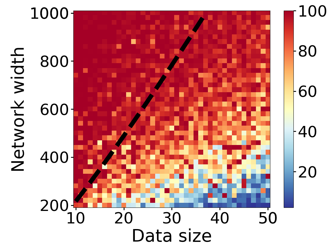
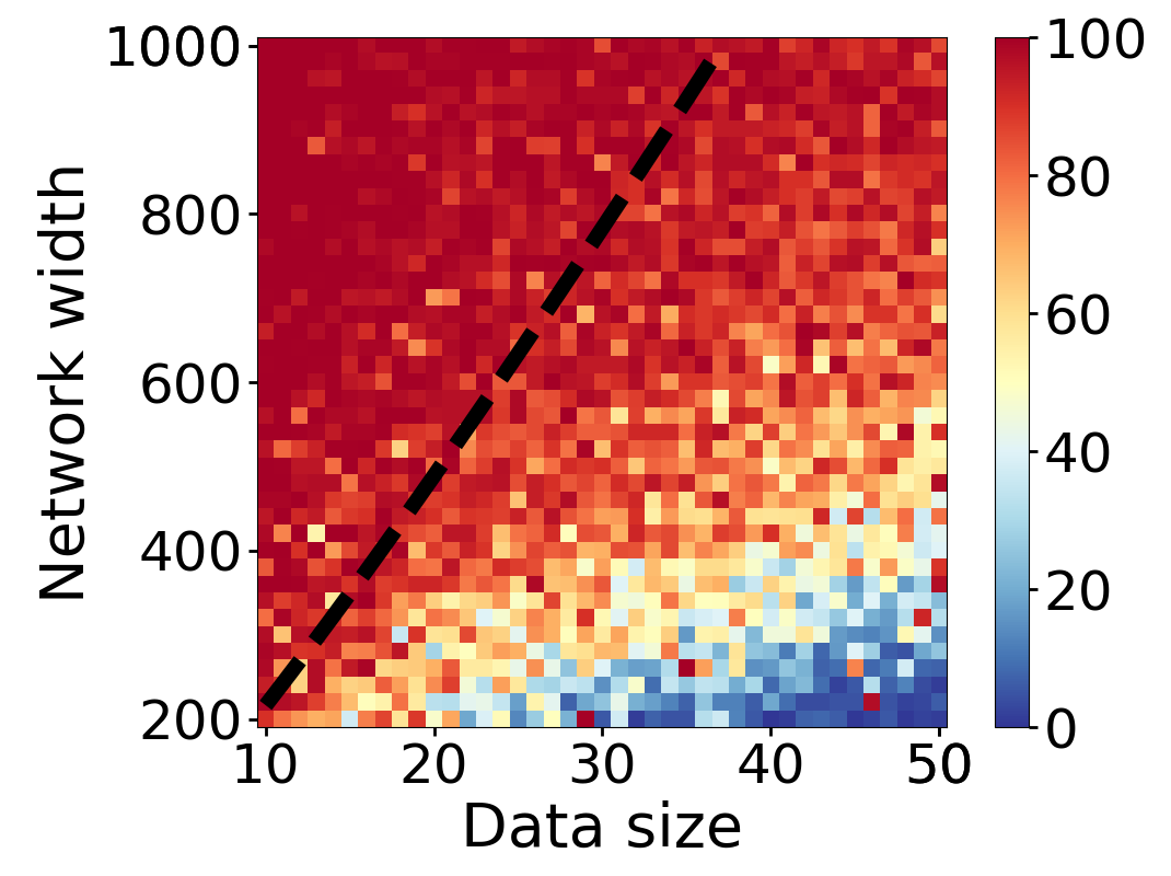
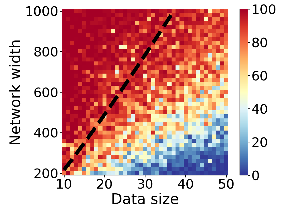
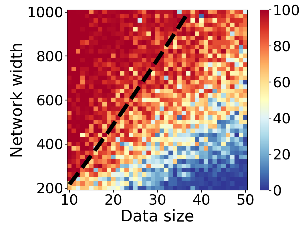
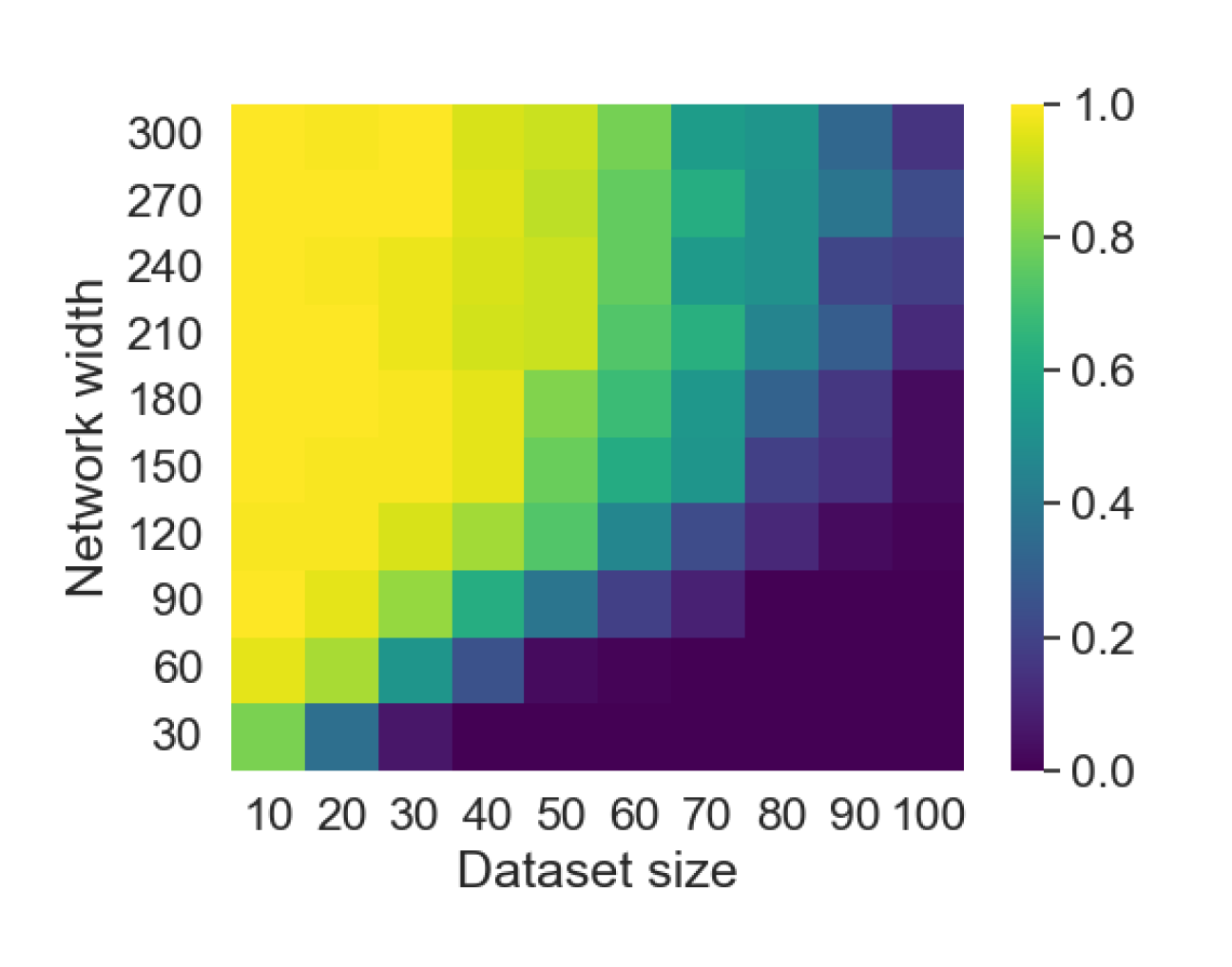
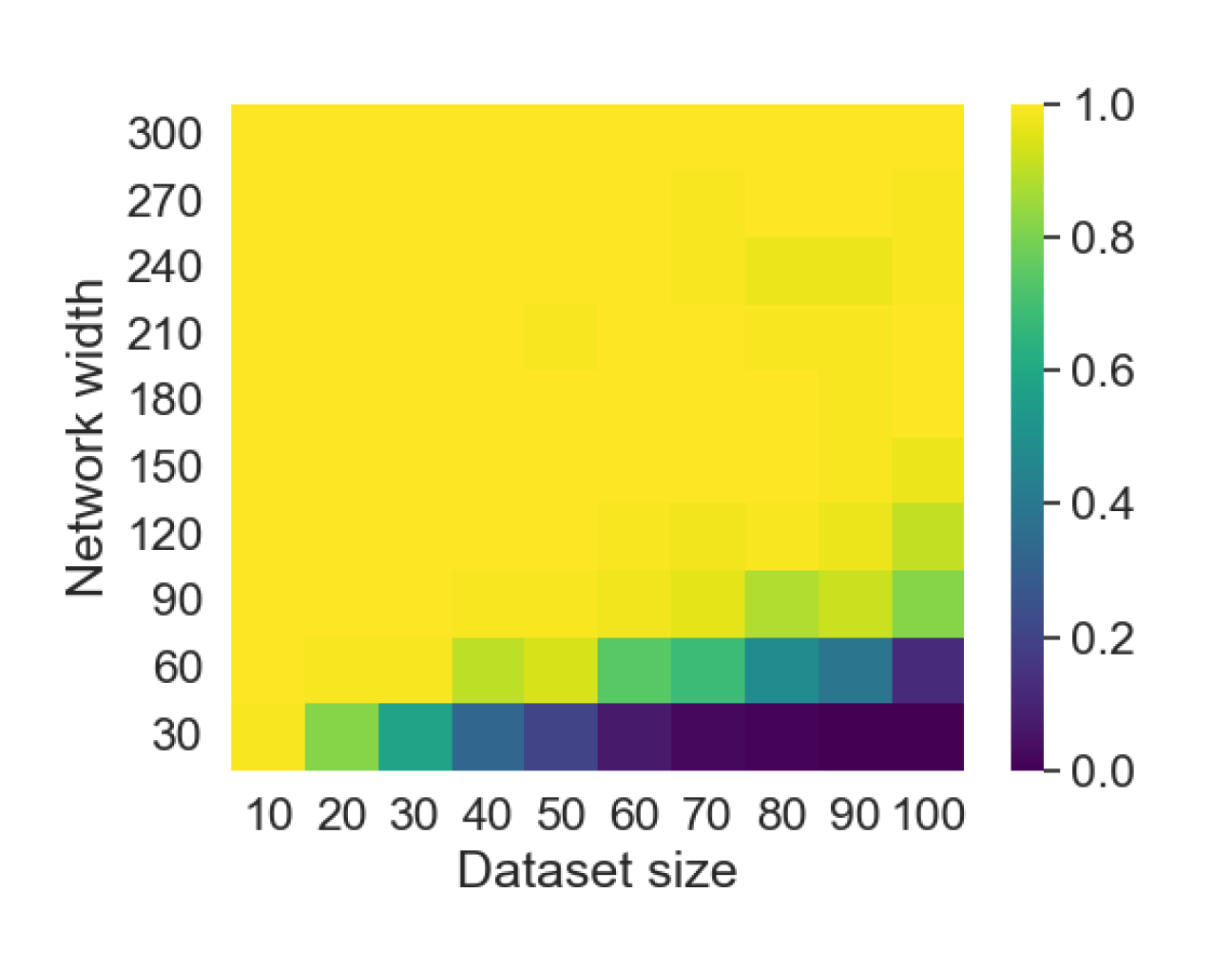
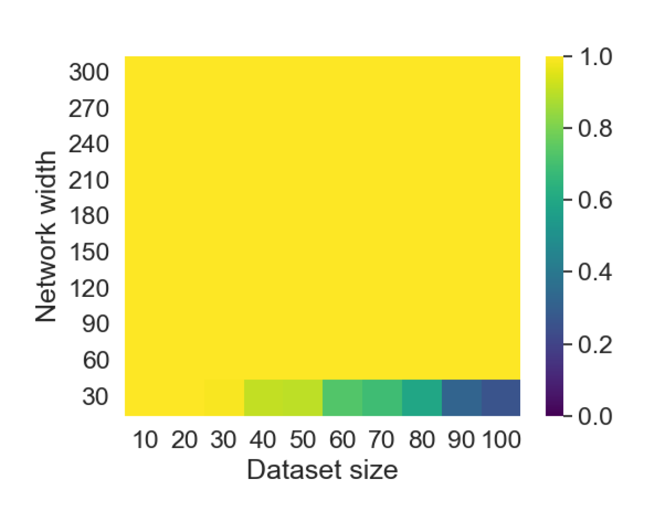
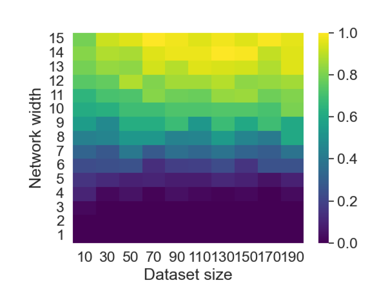
7 Experiments
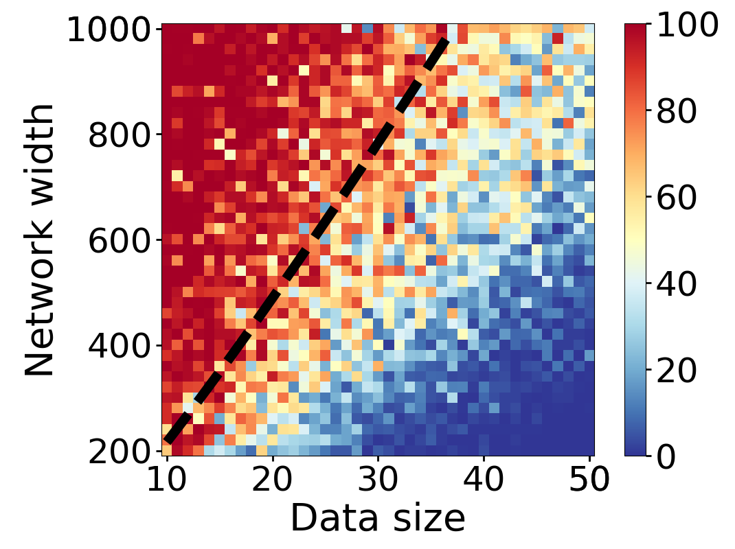
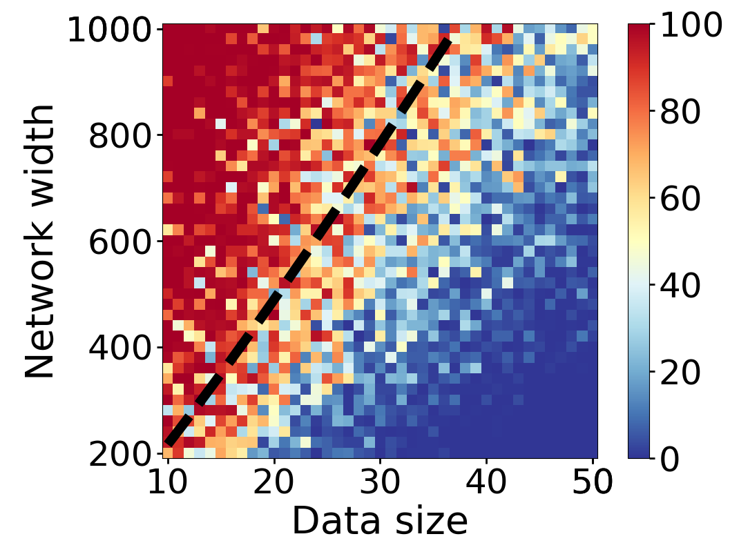
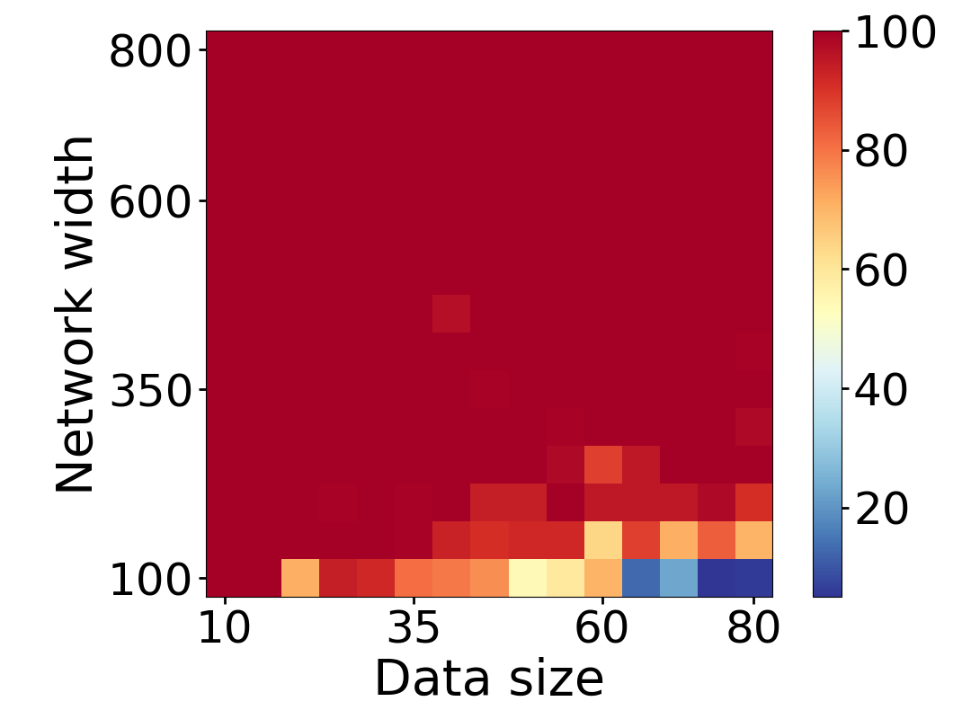
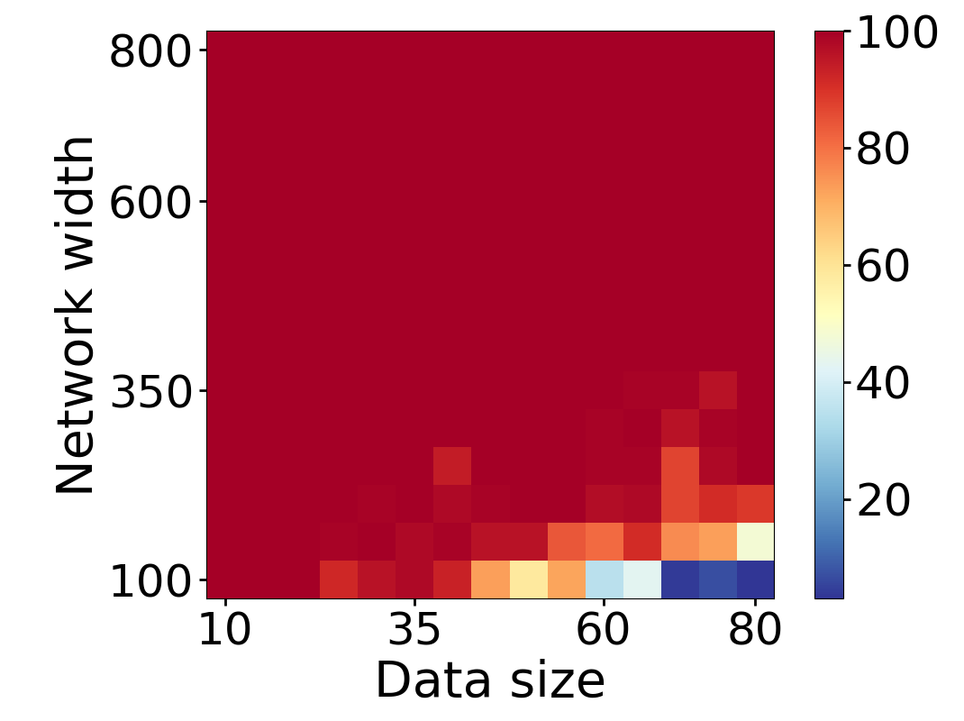
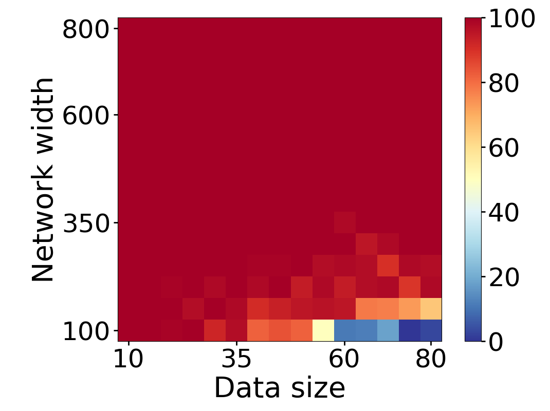
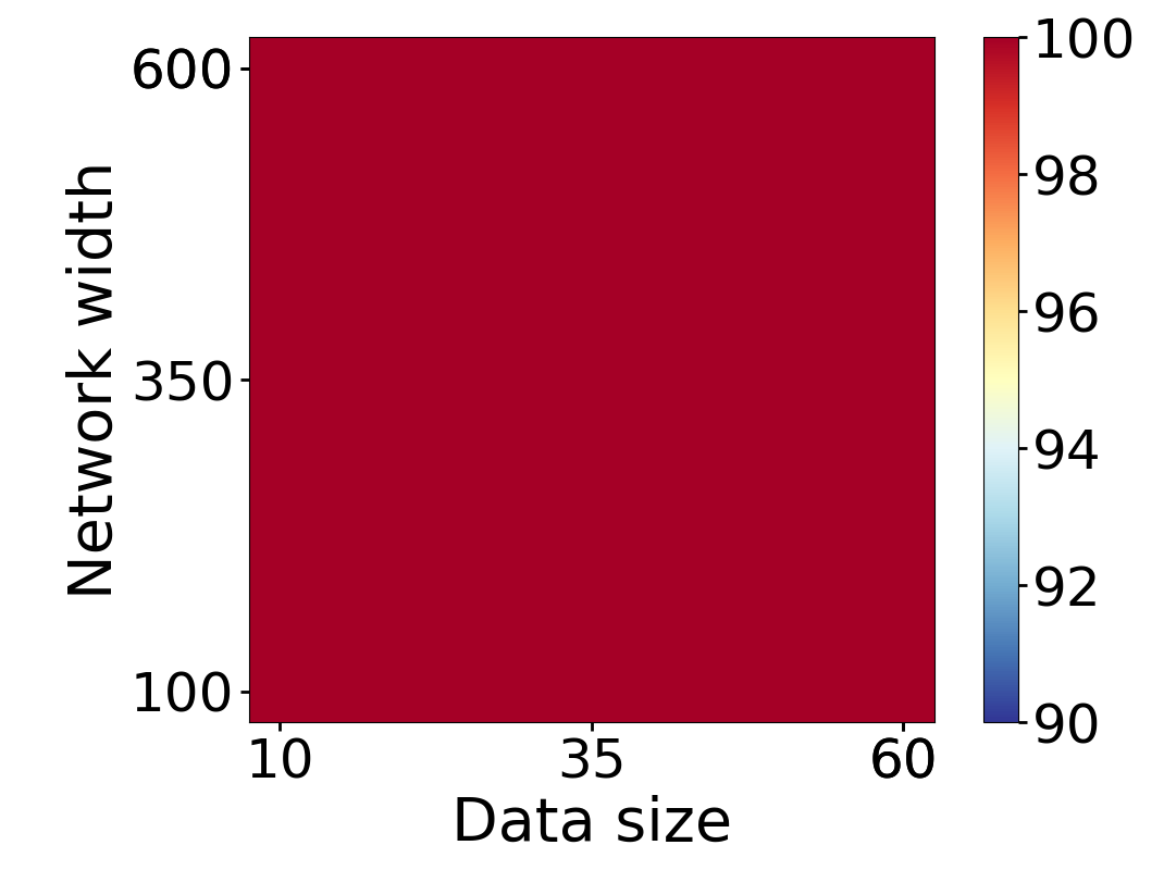
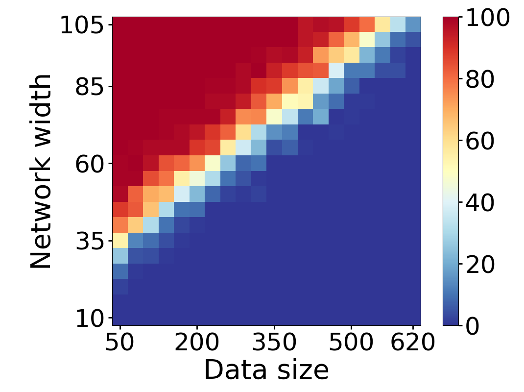
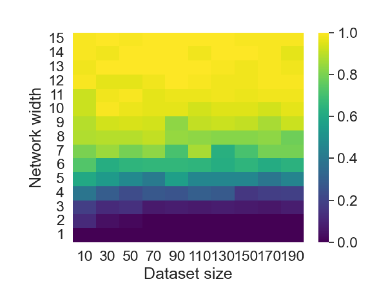
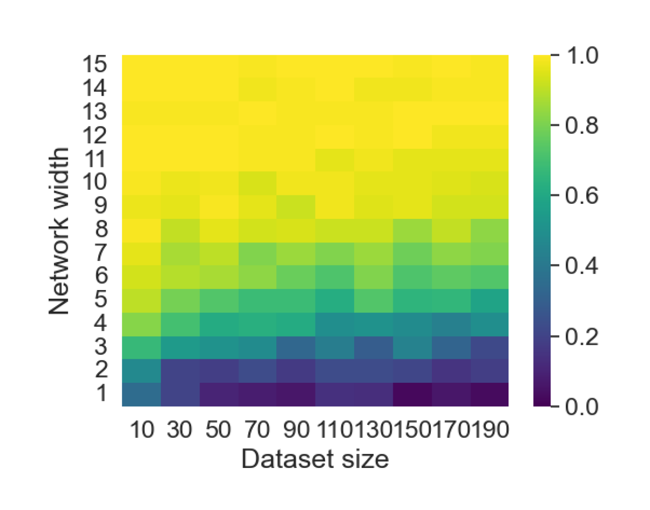
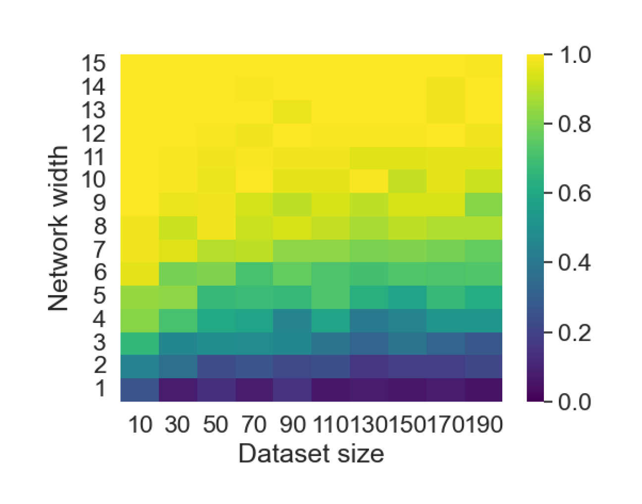
Here we empirically demonstrate that most regions of parameter space have a good optimization landscape by computing the rank of the Jacobian for two-layer neural networks. We initialize our network with random weights and biases sampled iid uniformly on . We evaluate the network on a random dataset whose entries are sampled iid Gaussian with mean 0 and variance 1. This gives us an activation region corresponding to the network evaluated at , and we record the rank of the Jacobian of that matrix. For each choice of , and , we run 100 trials and record the fraction of them which resulted in a Jacobian of full rank. The results are shown in Figures 1 and 2.
For different scalings of and , we observe different minimal widths needed for the Jacobian to achieve full rank with high probability. Figure 1 suggests that the minimum value of needed to achieve full rank increases linearly in the dataset size , and that the slope of this linear dependence decreases as the input dimension increases. This is exactly the behavior predicted by Theorem 2, which finds full rank regions for . Figure 2 operates in the regime , and shows that the necessary hidden dimension remains constant in the dataset size . This is again consistent with Theorem 5, whose bounds depend only on the ratio . Further supporting experiments, including those involving real-world data, are provided in Appendix G.
8 Conclusion
In this work we studied the loss landscape of both shallow and deep ReLU networks. The key takeaway is that mildly overparameterization in terms of network width suffices to ensure the loss landscape is favorable in the sense that bad local minima exist in only a small fraction of parameter space. In particular, using random matrix theory and combinatorial techniques we showed that most activation regions have no bad differentiable local minima by determining which regions have a full rank Jacobian. For univariate data we further proved that most regions contain a high-dimensional set of global minimizers and also showed illustrated that the same takeaway is true when also considering potential bad non-differentiable local minima on the boundaries between regions. Finally the combinatorial approach we adopted allowed us to prove results independent of the specific choice of initialization of parameters, or on the distribution of the dataset. There are a number of directions for improvement. Notably we obtain our strongest results for shallow one-dimensional input case, where we have a concrete grasp of the possible activation patterns; the case remains open. We leave strengthening our results concerning deep networks and high dimensional data to future work, and hope that our contributions inspire further exploration to address them.
Reproducibility statement
The computer implementation of the scripts needed to reproduce our experiments can be found at https://anonymous.4open.science/r/loss-landscape-4271.
Acknowledgments
This project has been supported by NSF CAREER 2145630, NSF 2212520, DFG SPP 2298 grant 464109215, ERC Starting Grant 757983, and BMBF in DAAD project 57616814.
References
- Anthony & Bartlett (1999) Martin Anthony and Peter L. Bartlett. Neural Network Learning: Theoretical Foundations. Cambridge University Press, 1999. URL https://doi.org/10.1017/CBO9780511624216.
- Auer et al. (1995) Peter Auer, Mark Herbster, and Manfred K. K Warmuth. Exponentially many local minima for single neurons. In D. Touretzky, M.C. Mozer, and M. Hasselmo (eds.), Advances in Neural Information Processing Systems, volume 8. MIT Press, 1995. URL https://proceedings.neurips.cc/paper_files/paper/1995/file/3806734b256c27e41ec2c6bffa26d9e7-Paper.pdf.
- Björner et al. (1999) Anders Björner, Michel Las Vergnas, Bernd Sturmfels, Neil White, and Gunter M. Ziegler. Oriented Matroids. Encyclopedia of Mathematics and its Applications. Cambridge University Press, 2 edition, 1999. URL https://www.cambridge.org/core/books/oriented-matroids/A34966F40E168883C68362886EF5D334.
- Bourgain et al. (2010) Jean Bourgain, Van H Vu, and Philip Matchett Wood. On the singularity probability of discrete random matrices. Journal of Functional Analysis, 258(2):559–603, 2010. URL https://www.sciencedirect.com/science/article/pii/S0022123609001955.
- Chen et al. (1993) An Mei Chen, Haw-minn Lu, and Robert Hecht-Nielsen. On the geometry of feedforward neural network error surfaces. Neural Computation, 5(6):910–927, 1993. URL https://ieeexplore.ieee.org/document/6796044.
- Chizat et al. (2019) Lénaïc Chizat, Edouard Oyallon, and Francis Bach. On lazy training in differentiable programming. In H. Wallach, H. Larochelle, A. Beygelzimer, F. d'Alché-Buc, E. Fox, and R. Garnett (eds.), Advances in Neural Information Processing Systems, volume 32. Curran Associates, Inc., 2019. URL https://proceedings.neurips.cc/paper_files/paper/2019/file/ae614c557843b1df326cb29c57225459-Paper.pdf.
- Cooper (2021) Yaim Cooper. Global minima of overparameterized neural networks. SIAM Journal on Mathematics of Data Science, 3(2):676–691, 2021. URL https://doi.org/10.1137/19M1308943.
- Cover (1964) Thomas M. Cover. Geometrical and Statistical Properties of Linear Threshold Devices. PhD thesis, Stanford Electronics Laboratories Technical Report #6107-1, May 1964. URL https://isl.stanford.edu/~cover/papers/paper1.pdf.
- Cover (1965) Thomas M. Cover. Geometrical and statistical properties of systems of linear inequalities with applications in pattern recognition. IEEE Transactions on Electronic Computers, EC-14(3):326–334, 1965.
- Dalcin et al. (2011) Lisandro D Dalcin, Rodrigo R Paz, Pablo A Kler, and Alejandro Cosimo. Parallel distributed computing using python. Advances in Water Resources, 34(9):1124–1139, 2011.
- Fukumizu & Amari (2000) Kenji Fukumizu and Shun-ichi Amari. Local minima and plateaus in hierarchical structures of multilayer perceptrons. Neural Networks, 13(3):317–327, 2000. URL https://www.sciencedirect.com/science/article/pii/S0893608000000095.
- Goldblum et al. (2020) Micah Goldblum, Jonas Geiping, Avi Schwarzschild, Michael Moeller, and Tom Goldstein. Truth or backpropaganda? an empirical investigation of deep learning theory. In International Conference on Learning Representations, 2020. URL https://openreview.net/forum?id=HyxyIgHFvr.
- Gori & Tesi (1992) Marco Gori and Alberto Tesi. On the problem of local minima in backpropagation. IEEE Transactions on Pattern Analysis and Machine Intelligence, 14(1):76–86, 1992. URL https://ieeexplore.ieee.org/document/107014.
- Grigsby et al. (2022) J. Elisenda Grigsby, Kathryn Lindsey, Robert Meyerhoff, and Chenxi Wu. Functional dimension of feedforward ReLU neural networks. arXiv preprint arXiv:2209.04036, 2022.
- Harris et al. (2020) Charles R Harris, K Jarrod Millman, Stéfan J Van Der Walt, Ralf Gommers, Pauli Virtanen, David Cournapeau, Eric Wieser, Julian Taylor, Sebastian Berg, Nathaniel J Smith, et al. Array programming with numpy. Nature, 585(7825):357–362, 2020.
- Harris (2013) Joe Harris. Algebraic geometry: A first course, volume 133. Springer Science & Business Media, 2013. URL https://link.springer.com/book/10.1007/978-1-4757-2189-8.
- He et al. (2020) Fengxiang He, Bohan Wang, and Dacheng Tao. Piecewise linear activations substantially shape the loss surfaces of neural networks. In International Conference on Learning Representations, 2020. URL https://openreview.net/forum?id=B1x6BTEKwr.
- He et al. (2015) Kaiming He, Xiangyu Zhang, Shaoqing Ren, and Jian Sun. Delving deep into rectifiers: Surpassing human-level performance on imagenet classification. In Proceedings of the IEEE international conference on computer vision, pp. 1026–1034, 2015. URL https://openaccess.thecvf.com/content_iccv_2015/html/He_Delving_Deep_into_ICCV_2015_paper.html.
- Hunter (2007) John D Hunter. Matplotlib: A 2D graphics environment. Computing in science & engineering, 9(03):90–95, 2007.
- Jacot et al. (2018) Arthur Jacot, Franck Gabriel, and Clement Hongler. Neural tangent kernel: Convergence and generalization in neural networks. In S. Bengio, H. Wallach, H. Larochelle, K. Grauman, N. Cesa-Bianchi, and R. Garnett (eds.), Advances in Neural Information Processing Systems, volume 31. Curran Associates, Inc., 2018. URL https://proceedings.neurips.cc/paper_files/paper/2018/file/5a4be1fa34e62bb8a6ec6b91d2462f5a-Paper.pdf.
- Joswig (2021) Michael Joswig. Essentials of tropical combinatorics, volume 219 of Graduate Studies in Mathematics. American Mathematical Society, Providence, RI, 2021. URL https://page.math.tu-berlin.de/~joswig/etc/index.html.
- Laurent & von Brecht (2018) Thomas Laurent and James von Brecht. The multilinear structure of ReLU networks. In Jennifer Dy and Andreas Krause (eds.), Proceedings of the 35th International Conference on Machine Learning, volume 80 of Proceedings of Machine Learning Research, pp. 2908–2916. PMLR, 10–15 Jul 2018. URL https://proceedings.mlr.press/v80/laurent18b.html.
- Liu (2021) Bo Liu. Understanding the loss landscape of one-hidden-layer relu networks. Knowledge-Based Systems, 220:106923, 2021. URL https://www.sciencedirect.com/science/article/pii/S0950705121001866.
- Montúfar et al. (2014) Guido Montúfar, Razvan Pascanu, Kyunghyun Cho, and Yoshua Bengio. On the number of linear regions of deep neural networks. In Z. Ghahramani, M. Welling, C. Cortes, N. Lawrence, and K.Q. Weinberger (eds.), Advances in Neural Information Processing Systems, volume 27. Curran Associates, Inc., 2014. URL https://proceedings.neurips.cc/paper_files/paper/2014/file/109d2dd3608f669ca17920c511c2a41e-Paper.pdf.
- Montúfar et al. (2022) Guido Montúfar, Yue Ren, and Leon Zhang. Sharp bounds for the number of regions of maxout networks and vertices of Minkowski sums. SIAM Journal on Applied Algebra and Geometry, 6(4):618–649, 2022. URL https://doi.org/10.1137/21M1413699.
- Nguyen (2019) Quynh Nguyen. On connected sublevel sets in deep learning. In Kamalika Chaudhuri and Ruslan Salakhutdinov (eds.), Proceedings of the 36th International Conference on Machine Learning, volume 97 of Proceedings of Machine Learning Research, pp. 4790–4799. PMLR, 09–15 Jun 2019. URL https://proceedings.mlr.press/v97/nguyen19a.html.
- Oymak & Soltanolkotabi (2019) Samet Oymak and Mahdi Soltanolkotabi. Toward moderate overparameterization: Global convergence guarantees for training shallow neural networks. IEEE Journal on Selected Areas in Information Theory, 1:84–105, 2019.
- Paszke et al. (2019) Adam Paszke, Sam Gross, Francisco Massa, Adam Lerer, James Bradbury, Gregory Chanan, Trevor Killeen, Zeming Lin, Natalia Gimelshein, Luca Antiga, et al. Pytorch: An imperative style, high-performance deep learning library. Advances in neural information processing systems, 32, 2019.
- Phuong & Lampert (2020) Mary Phuong and Christoph H. Lampert. Functional vs. parametric equivalence of ReLU networks. In International Conference on Learning Representations, 2020. URL https://openreview.net/forum?id=Bylx-TNKvH.
- Poston et al. (1991) T. Poston, C.-N. Lee, Y. Choie, and Y. Kwon. Local minima and back propagation. In IJCNN-91-Seattle International Joint Conference on Neural Networks, volume ii, pp. 173–176 vol.2, 1991. URL https://ieeexplore.ieee.org/document/155333.
- Safran & Shamir (2016) Itay Safran and Ohad Shamir. On the quality of the initial basin in overspecified neural networks. In Maria Florina Balcan and Kilian Q. Weinberger (eds.), Proceedings of The 33rd International Conference on Machine Learning, volume 48 of Proceedings of Machine Learning Research, pp. 774–782, New York, New York, USA, 20–22 Jun 2016. PMLR. URL https://proceedings.mlr.press/v48/safran16.html.
- Safran & Shamir (2018) Itay Safran and Ohad Shamir. Spurious local minima are common in two-layer ReLU neural networks. In Jennifer Dy and Andreas Krause (eds.), Proceedings of the 35th International Conference on Machine Learning, volume 80 of Proceedings of Machine Learning Research, pp. 4433–4441. PMLR, 10–15 Jul 2018. URL https://proceedings.mlr.press/v80/safran18a.html.
- Sakurai (1998) Akito Sakurai. Tight bounds for the VC-dimension of piecewise polynomial networks. In M. Kearns, S. Solla, and D. Cohn (eds.), Advances in Neural Information Processing Systems, volume 11. MIT Press, 1998. URL https://proceedings.neurips.cc/paper_files/paper/1998/file/f18a6d1cde4b205199de8729a6637b42-Paper.pdf.
- Schläfli (1950) Ludwig Schläfli. Theorie der vielfachen Kontinuität, pp. 167–387. Springer Basel, Basel, 1950. URL https://doi.org/10.1007/978-3-0348-4118-4_13.
- Sharifnassab et al. (2020) Arsalan Sharifnassab, Saber Salehkaleybar, and S. Jamaloddin Golestani. Bounds on over-parameterization for guaranteed existence of descent paths in shallow ReLU networks. In International Conference on Learning Representations, 2020. URL https://openreview.net/forum?id=BkgXHTNtvS.
- Simsek et al. (2021) Berfin Simsek, François Ged, Arthur Jacot, Francesco Spadaro, Clement Hongler, Wulfram Gerstner, and Johanni Brea. Geometry of the loss landscape in overparameterized neural networks: Symmetries and invariances. In Marina Meila and Tong Zhang (eds.), Proceedings of the 38th International Conference on Machine Learning, volume 139 of Proceedings of Machine Learning Research, pp. 9722–9732. PMLR, 18–24 Jul 2021. URL https://proceedings.mlr.press/v139/simsek21a.html.
- Sontag & Sussmann (1989) Eduardo Sontag and Héctor J. Sussmann. Backpropagation can give rise to spurious local minima even for networks without hidden layers. Complex Syst., 3, 1989. URL https://www.complex-systems.com/abstracts/v03_i01_a07/.
- Soudry & Carmon (2016) Daniel Soudry and Yair Carmon. No bad local minima: Data independent training error guarantees for multilayer neural networks. arXiv preprint arXiv:1605.08361, 2016.
- Swirszcz et al. (2017) Grzegorz Swirszcz, Wojciech Marian Czarnecki, and Razvan Pascanu. Local minima in training of deep networks, 2017. URL https://openreview.net/forum?id=Syoiqwcxx.
- Tian (2017) Yuandong Tian. An analytical formula of population gradient for two-layered ReLU network and its applications in convergence and critical point analysis. In Doina Precup and Yee Whye Teh (eds.), Proceedings of the 34th International Conference on Machine Learning, volume 70 of Proceedings of Machine Learning Research, pp. 3404–3413. PMLR, 06–11 Aug 2017. URL https://proceedings.mlr.press/v70/tian17a.html.
- Wang et al. (2022) Yifei Wang, Jonathan Lacotte, and Mert Pilanci. The hidden convex optimization landscape of regularized two-layer reLU networks: an exact characterization of optimal solutions. In International Conference on Learning Representations, 2022. URL https://openreview.net/forum?id=Z7Lk2cQEG8a.
- Yun et al. (2019a) Chulhee Yun, Suvrit Sra, and Ali Jadbabaie. Small ReLU networks are powerful memorizers: a tight analysis of memorization capacity. In H. Wallach, H. Larochelle, A. Beygelzimer, F. d'Alché-Buc, E. Fox, and R. Garnett (eds.), Advances in Neural Information Processing Systems, volume 32. Curran Associates, Inc., 2019a. URL https://proceedings.neurips.cc/paper_files/paper/2019/file/dbea3d0e2a17c170c412c74273778159-Paper.pdf.
- Yun et al. (2019b) Chulhee Yun, Suvrit Sra, and Ali Jadbabaie. Small nonlinearities in activation functions create bad local minima in neural networks. In International Conference on Learning Representations, 2019b. URL https://openreview.net/forum?id=rke_YiRct7.
- Zaslavsky (1975) Thomas Zaslavsky. Facing up to Arrangements: Face-Count Formulas for Partitions of Space by Hyperplanes. American Mathematical Society: Memoirs of the American Mathematical Society. American Mathematical Society, 1975. URL https://books.google.com/books?id=K-nTCQAAQBAJ.
- Zhang et al. (2018) Liwen Zhang, Gregory Naitzat, and Lek-Heng Lim. Tropical geometry of deep neural networks. In Jennifer Dy and Andreas Krause (eds.), Proceedings of the 35th International Conference on Machine Learning, volume 80 of Proceedings of Machine Learning Research, pp. 5824–5832, Stockholmsmässan, Stockholm Sweden, 10–15 Jul 2018. PMLR. URL http://proceedings.mlr.press/v80/zhang18i.html.
- Zhou & Liang (2018) Yi Zhou and Yingbin Liang. Critical points of linear neural networks: Analytical forms and landscape properties. In International Conference on Learning Representations, 2018. URL https://openreview.net/forum?id=SysEexbRb.
Appendix A Details on counting activation regions with no bad local minima
We provide the proofs of the results presented in Section 3.
Proof of Lemma 4.
Suppose that . Since the entries of are nonzero, the following are equivalent:
So the kernel of the matrix whose -th row is is equal to the kernel of the matrix whose -th row is . It follows that
∎
Proof of Theorem 5.
Suppose that . Consider a matrix , which corresponds to one of the theoretically possible activation pattern of all units across all input examples, and denote its columns by . For any given input dataset , the function is piecewise linear in . More specifically, on each activation region , is a linear map in of the form
So on the Jacobian of is given by the Khatri-Rao (columnwise Kronecker) product
| (2) |
In particular, is of full rank on exactly when the set
consists of linearly independent elements of , since . By Lemma 4, this is equivalent to the set
consisting of linearly independent vectors, or in another words, the Khatri-Rao product having full rank.
For a given consider the set
The expression corresponds to in the case that . Suppose that is large enough that . We will show that for most , is non-empty and in fact contains almost every . We may partition into subsets such that for all and partition the set of columns of accordingly into blocks for all . Let us form a matrix whose columns are the . We will use a probabilistic argument. For this, consider the entries of as being iid Bernoulli random variables with parameter . We may extend to a random matrix whose entries are iid Bernoulli random variables with parameter . By Theorem 3, will be singular with probability at most
where is a universal constant. Whenever is nonsingular, the vectors are linearly independent. Using a simple union bound, we have
Now suppose that are linearly independent for all . Let be the standard basis of . Since , there exists such that whenever . For such an , we claim that the set
consists of linearly independent elements of . To see this, suppose that there exist such that
Then
The above equation can only hold if
By the linear independence of , this implies that for all . This shows that the elements are linearly independent for a particular whenever the are all linearly independent. In other words, is non-empty with probability at least when the activation region is chosen uniformly at random.
Let us define
We have shown that if is chosen uniformly at random from , then with high probability. Note that is defined in terms of polynomials of not vanishing, so is the complement of a Zariski-closed subset of . Let
Then is a Zariski-open set of full measure, since it is a finite intersection of non-empty Zariski-open sets (which are themselves of full measure by Lemma 1). If and , then is of full rank for all , and therefore all local minima in will be global minima by Lemma 2. So if we take and such that
and choose uniformly at random, then with probability at least
will have no bad local minima. We rephrase this as a combinatorial result: if satisfies the same bounds above, then for generic datasets we have the following: for all but at most activation regions , has no bad local minima. The theorem follows. ∎
The argument that we used to prove that the Jacobian is full rank for generic data can be applied to arbitrary binary matrices. The proof is exactly the same as the sub-argument in the proof of Theorem 5.
Lemma 18.
For generic datasets , the following holds. Let for . Suppose that there exists a partition of into subsets such that for all ,
Then
Appendix B Details on counting non-empty activation regions
We provide the proofs of the results presented in Section 3. The subdivisions of parameter space by activation properties of neurons is classically studied in VC-dimension computation (Cover, 1965; Sakurai, 1998; Anthony & Bartlett, 1999). This has similarities to the analysis of linear regions in input space for neural networks with piecewise linear activation functions (Montúfar et al., 2014).
Proof of Proposition 6.
Consider the map that takes the input weights of a single ReLU to its activation values over input data points given by the columns of . This can equivalently be interpreted as a map taking an input vector to the activation values of ReLUs with input weights given by the columns of . The linear regions of the latter correspond to the (full-dimensional) regions of a central arrangement of hyperplanes in with normals . Denote the number of such regions by . If the columns of are in general position in a -dimensional linear space, meaning that they are contained in a -dimensional linear space and any columns are linearly independent, then
| (3) |
This is a classic result that can be traced back to the work of Schläfli (1950), and which also appeared in the discussion of linear threshold devices by Cover (1964).
Now for a layer of ReLUs, each unit has its parameter space subdivided by an equivalent hyperplane arrangement that is determined solely by . Since all units have individual parameters, the arrangement of each unit essentially lives in a different set of coordinates. In turn, the overall arrangement in the parameter space of all units is a so-called product arrangement, and the number of regions is . This conclusion is sufficiently intuitive, but it can also be derived from Zaslavsky (1975, Lemma 4A3). If the input data is in general position in a -dimensional linear subspace of the input space, then we can substitute equation 3 into and obtain the number of regions stated in the proposition. ∎
We are also interested in the specific identity of the non-empty regions; that is, the sign patterns that are associated with them. As we have seen above, the set of sign patterns of a layer of units is the -Cartesian power of the set of sign patterns of an individual unit. Therefore, it is sufficient to understand the set of sign patterns of an individual unit; that is, the set of dichotomies that can be computed over the columns of by a bias-free simple perceptron . Note that this subsumes networks with biases as the special case where the first row of consists of ones, in which case the first component of the weight vector can be regarded as the bias. Let be the matrix whose rows are the different possible dichotomies . If we extend the definition of dichotomies to allow not only and but also zeros for the case that data points fall on the decision boundary, then we obtain a matrix that is referred to as the oriented matroid of the vector configuration , and whose rows are referred to as the covectors of (Björner et al., 1999). This is also known as the list of sign sequences of the faces of the hyperplane arrangement.
To provide more intuitions for Proposition 8, we give a self-contained proof below.
Proof of Proposition 8.
For each unit, the parameter space is subdivided by an arrangement of hyperplanes with normals given by , . A weight vector is in the interior of the activation region with pattern if and only if for all . Equivalently,
| for all with | |||
This means that is a point where the function attains the maximum value among of all linear functions with gradients given by sums of s, meaning that at this function attains the same value as
| (4) |
Dually, the linear function attains its maximum over the polytope
| (5) |
precisely at . In other words, is an extreme point or vertex of with a supporting hyperplane with normal . For a polytope , the normal cone of at a point is defined as the set of such that for all . For any let us denote by the vector with ones at components in and zeros otherwise. Then the above discussion shows that the activation region with is the interior of the normal cone of at . In particular, the activation region is non empty if and only if is a vertex of .
To conclude, we show that is a Minkowski sum of line segments,
To see this note that if and only if there exist , with
where and . Thus, if and only if is a sum of points , meaning that as was claimed. ∎
The polytope equation 5 may be regarded as the Newton polytope of the piecewise linear convex function equation 4 in the context of tropical geometry (Joswig, 2021). This perspective has been used to study the linear regions in input space for ReLU (Zhang et al., 2018) and maxout networks (Montúfar et al., 2022).
We note that each vertex of a Minkowski sum of polytopes is a sum of vertices of the summands , but not every sum of vertices of the results in a vertex of . Our polytope is a sum of line segments, which is a type of polytope known as a zonotope. Each vertex of takes the form , where each is a vertex of , either the zero vertex or the nonzero vertex , and is naturally labeled by a vector that indicates the s for which . A zonotope can be interpreted as the image of a cube by a linear map; in our case it is the projection of the -cube into by the matrix . The situation is illustrated in Figure 3.
Example 19 (Non-empty activation regions for 1-dimensional inputs).
In the case of one-dimensional inputs and units with biases, the parameter space of each unit is . We treat the data as points , where the first coordinate is to accommodate the bias. For generic data (i.e., no data points on top of each other), the polytope is a polygon with vertices. The vertices have labels indicating, for each , the subsets containing the largest respectively smallest elements in the dataset with respect to the non-bias coordinate.
Appendix C Details on counting non-empty activation regions with no bad minima
We provide the proofs of the statements in Section 4.
Proof of Lemma 9.
First we establish that the rows of the matrices corresponding to non-empty activation regions must be step vectors. To this end, assume and for an arbitrary row let . If for all , then the -th row of is a step vector equal to either or . Otherwise, there exists a minimal such that . We proceed by contradiction to prove in this setting that for all . Suppose there exists a such that , then as and this implies that the following two inequalities are simultaneously satisfied,
However, these inequalities clearly contradict one another and therefore we conclude is a step vector equal to either or
Conversely, assume the rows of are all step vectors. We proceed to prove is non-empty under this assumption by constructing such that for all and any row . To this end, let . First, consider the case where for all . If then with and it follows that
for all . If , then with and we have
for all . Otherwise, suppose is not constant: then by construction there exists a such that for all and for all . Letting
then for any
Thus, for any with step vector rows, given a dataset consisting distinct one dimensional points we can construct network whose preactivations correspond to the activation pattern encoded by .
In summary, given a fixed, distinct one dimensional dataset we have established a one-to-one correspondence between the non-empty activation regions and the set of binary matrices whose rows are step vectors. For convenience we refer to these as row-step matrices. As there are step vector rows of dimension and rows in , then there are binary row-step matrices and hence non-empty activation regions. ∎
Proof of Lemma 11.
By the union bound,
So if ,
This concludes the proof. ∎
Proof of Theorem 10.
Consider a dataset consisting of distinct data points. Without loss of generality we may index these points such that
Now consider a matrix whose rows are step vectors and which therefore corresponds to a non-empty activation region by Lemma 9. As in the proof of Theorem 5, denote its columns by for . On , the Jacobian of with respect to is given by
We claim that if has full rank, then has full rank for all with the entries of nonzero. To see this, suppose that is of full rank, and that
for some . Then for all ,
But is of full rank, so this implies that for all . As a result, if is full rank then is full rank, and in particular is rank. Therefore, to show most non-empty activation regions have no bad local minima, it suffices to show most non-empty activation regions are defined by a full rank binary matrix .
To this end, if is a binary matrix with step vector rows, we say that is diverse if it satisfies the following properties:
-
1.
For all , there exists such that .
-
2.
There exists such that .
We proceed by i) showing all diverse matrices are of full rank and then ii) non-empty activation regions are defined by a diverse matrix. Suppose is diverse and denote the span of the rows of by . Then and for each either or is in . Observe if then , therefore for all . As the set of vectors
forms a basis of we conclude that all diverse matrices are full rank.
Now we show most binary matrices with step vector rows are diverse. Let be a random binary matrix whose rows are selected mutually iid from the set of all step vectors. For , let be defined as follows: if for some , we define ; if , then we define ; otherwise, we define . By definition is diverse if and only if
As the rows of are chosen uniformly at random from the set of all step vectors, the are iid and
for all , then by Lemma 11, if ,
This holds for a randomly selected matrix with step vector rows. Translating this into a combinatorial statement, we see for all but at most a fraction of matrices with step vector rows are diverse. Furthermore, in each activation region corresponding to a diverse the Jacobian is full rank and every differentiable critical point of is a global minimum. ∎
Proof of Theorem 12.
Let . We define the following two sets of neurons based on the sign of their output weight,
Suppose that . Furthermore, without loss of generality, we index the points in the dataset such that
Now consider a matrix whose rows are step vectors, then by Lemma 9 corresponds to a non-empty activation region. We say that is complete if for all and there exists such that and . We first show that if is complete, then there exists a global minimizer in . Consider the linear map defined by
Note for then . As proved in Lemma 20, for every there exists such that . In particular, this means that is surjective and therefore contains zero-loss global minimizers. Define
then and by the rank-nullity theorem
We therefore conclude that if is complete, then is the restriction of a -dimensional linear subspace to the open set . This is equivalent to being an affine set of codimension as claimed.
To prove the desired result it therefore suffices to show that most binary matrices with step vector rows are complete. Let be a random binary matrix whose rows are selected mutually iid uniformly at random from the set of all step vectors. For and let be defined as follows: if for some then , otherwise . Observe that is complete if and only if
Since there are step vectors,
for all . So by the union bound and Lemma 11,
As this holds for a matrix with step vectors chosen uniformly at random, it therefore follows that all but at most a fraction of such matrices are complete. This concludes the proof. ∎
Lemma 20.
Let be complete, and let be an input dataset with distinct points. Then for any , there exists such that .
Proof.
If is complete then there exist row indices and such that for all and the -th row of is equal to with . For , we define
We will construct weights and biases such that and . For , we define and arbitrarily such that
for all . Note by Lemma 9 that this is possible as each is a step vector. Therefore, in order to show the desired result it suffices only to appropriately construct for . To this end we proceed using the following sequence of steps.
-
1.
First we separately consider the contributions to the output of the network coming from the slack neurons, those with index , and the key neurons, those with index . For , we denote the residual of the target leftover after removing the corresponding output from the slack part of the network as . We then recursively build a sequence of functions in such a manner that for all .
-
2.
Based on this construction, we select the parameters of the key neurons, i.e., for , and prove .
-
3.
Finally, using these parameters and the function we show .
Step 1: for we define the residual
| (6) |
For , consider the values , and the functions , defined recursively across the dataset as
Observe for all that and
In particular, if and otherwise. Moreover, for all ,
We claim that for all , . For the case , we compute
For ,
Hence, for all .
Step 2: based on the construction above we define for . For and , we define
Now we show that this pair satisfies the desired properties. By construction, we have
for , . If , then we can write for some , . Then
where the second-to-last line follows from the construction of and and the last line follows from the fact that .
Step 3: finally, we show that . For ,
where the last line follows from (6). By the definition of and , this is equal to
By construction , so the above is equal to
In conclusion, we have therefore successfully identified weights and biases such that . ∎
Proof of Theorem 13.
We say that a binary matrix with step vector rows is diverse if for all , there exists such that . Suppose that is a binary matrix uniformly selected among all binary matrices with step vector rows. Define the random variables by if for some , and otherwise. Since the rows of are iid, the are iid. Moreover, for each , we have . So by Lemma 11, if
then with probability at least ,
This means that for each , there exists such that . In other words, is diverse. Since we chose uniformly at random among all binary matrices with step vector rows, it follows that all but a fraction of such matrices are diverse.
Now it suffices to show that when is diverse, every local minimum of in is a global minimum. Note that is continuously differentiable with respect to everywhere. We will show that has rank for all . Since is diverse, there exist such that for all , . Consider the submatrix of generated by the rows . That is,
Then
so the entries of are non-negative, and
Hence, is upper triangular with positive entries on its diagonals, implying that . Since is a submatrix of , we have as well. Now suppose that is a local minimum of . Then
Since has rank , this implies that , and so is a global minimizer of . So whenever is diverse, the region has no bad local minima. This concludes the proof. ∎
Appendix D Function space on one-dimensional data
We have studied activation regions in parameter space over which the Jacobian has full rank. We can give a picture of what the function space looks like as follows. We describe the function space of a ReLU over the data and based on this the function space of a network with a hidden layer of ReLUs.
Consider a single ReLU with one input with bias on input data points in . Equivalently, this is as a ReLU with two input dimensions and no bias on input data points in . For fixed , denote by the vector of outputs on all input data points, and by the set of all such vectors for any choice of the parameters. For a network with a single output coordinate, this is a subset of . As before, without loss of generality we sort the input data as (according to the non-constant component). We will use notation of the form . Further, we write , which is a solution of the linear equation . Recall that a polyline is a list of points with line segments drawn between consecutive points.
Since the parametrization map is piecewise linear, the function space is the union of the images of the Jacobian over the parameter regions where it is constant. In the case of a single ReLU one quickly verifies that, for , , and for , . For general , there will be equality and inequality constraints, coming from the bounded rank of the Jacobian and the boundaries of the linear regions in parameter space.
The function space of a single ReLU on and data points is illustrated in Figure 4.
For a single ReLU, there are non-empty activation regions in parameter space. One of them has Jacobian rank 0 and is mapped to the 0 function, two others have Jacobian rank 1 and are mapped to non-negative scalar multiples of the coordinate vectors and , and the other regions have Jacobian rank 2 and are each mapped to the set of non-negative scalar multiples of a line segment in the polyline. Vertices in the list equation 7 correspond to the extreme rays of the linear pieces of the function space of the ReLU. They are the extreme rays of the cone of non-negative convex functions on . Here a function on is convex if . A non-negative sum of ReLUs is always contained in the cone of non-negative convex functions, which over data points is an -dimensional convex polyhedral cone. For an overparameterized network, if an activation region in parameter space has full rank Jacobian, then that region maps to an -dimensional polyhedral cone. It contains a zero-loss minimizer if and only if the corresponding cone intersects the output data vector .
Proposition 21 (Function space on one-dimensional data).
Let be a list of distinct points in sorted in increasing order with respect to the second coordinate.
-
•
Then the set of functions a ReLU represents on is a polyhedral cone consisting of functions , where and is an element of the polyline with vertices
(7) -
•
The set of functions represented by a sum of ReLUs consists of non-negative scalar multiples of convex combinations of any points on this polyline.
-
•
The set of functions represented by arbitrary linear combinations of ReLUs consists of arbitrary scalar multiples of affine combinations of any points on this polyline.
Proof of Proposition 21.
Consider first the case of a single ReLU. We write for the input data points in . The activation regions in parameter space are determined by the arrangement of hyperplanes . Namely, the unit is active on the input data point if and only if the parameter is contained in the half-space and it is inactive otherwise. We write , which is a row vector that satisfies . We write for a vector in with ones at the coordinates and zeros elsewhere, and write for the matrix in where we substitute columns of whose index is not in by zero columns.
With these notations, in the following table we list, for each of the non-empty activation regions, the rank of the Jacobian, the activation pattern, the description of the activation region as an intersection of half-spaces, the extreme rays of the activation region, and the extreme rays of the function space represented by the activation region, which is simply the image of the Jacobian over the activation region.
The situation is illustrated in Figure 5 (see also Figure 4). On one of the parameter regions the unit is inactive on all data points so that the Jacobian has rank 0 and maps to 0. There are precisely two parameter regions where the unit is active on just one data point, or , so that the Jacobian has rank 1 and maps to non-negative multiples of and , respectively. On all the other parameter regions the unit is active at least on two data points. On those data points where the unit is active it can adjust the slope and intercept by local changes of the bias and weight and these are all the available degrees of freedom, so that the Jacobian has rank 2. These regions map to two-dimensional cones in function space. To obtain the extreme rays of these cones, we just evaluate the Jacobian on the two extreme rays of the activation region. This gives us item 1 in the proposition.
Consider now ReLUs. Recall that the Minkowski sum of two sets in a vector space is defined as . An activation region with activation pattern for all units corresponds to picking one region with pattern for each of the units, . Since the parametrization map is linear on the activation region, the overall computed function is simply the sum of the functions computed by each of the units,
Here is the overall function and is the function computed by the th unit. The parameters and activation regions of all units are independent of each other. Thus
Here we write for the function space of the th unit over its activation region . This is a cone and thus it is closed under nonegative scaling,
Thus, for an arbitrary linear combination of ReLUs we have
Here is an arbitrary function represented by the th unit. We have and . Thus if satisfies , then , and hence is an affine combination of the functions . If all are non-negative, then and the affine combination is a convex combination. Each of the summands is an element of the function space of a single ReLU with entries adding to one.
In conclusion, the function space of a network with one hidden layer of ReLUs with non-negative output weights is the set of non-negative scalar multiples of functions in the convex hull of any functions in the normalized function space of a single ReLU. For a network with arbitrary output weights we obtain arbitrary scalar multiples of the affine hulls of any functions in the normalized function space of a single ReLU. This is what was claimed in items 2 and 3, respectively. ∎
Appendix E Details on loss landscapes of deep networks
We provide details and proofs of the results in Section 5. We say that a binary matrix is non-repeating if its columns are distinct.
Proposition 22.
Let be an input dataset with distinct points. Suppose that is an activation pattern such that has rank , and such that is non-repeating for all . Then for all , has rank .
Proof.
Suppose that is an activation pattern satisfying the stated properties. We claim that for all , , and with , that . We prove by induction on . The base case holds by assumption. Suppose that the claim holds for some . By assumption, is non-repeating, so the columns and are not equal. Let be such that . Then, since ,
This implies that
or in other words
So , proving the claim by induction.
Now we consider the gradient of with respect to the -th layer. Let be defined by , and for let denote the -th column of . Let denote the rows of . Then for all ,
By Lemma 4, the rank of this matrix is equal to the rank of the matrix
But has rank by assumption, so the set is linearly independent, implying that the above matrix is full rank. Hence, has full rank, and so has full rank. ∎
Now we count the number of activation patterns which satisfy the assumptions of Proposition 22 and hence correspond to regions with full rank Jacobian.
Lemma 23.
Suppose that has entries chosen iid uniformly from . If
then with probability at least , is non-repeating.
Proof.
For any with ,
So
If
then the above expression is at least . ∎
Lemma 24.
Suppose that has entries chosen iid uniformly from . If
then with probability at least , has rank .
Proof.
Suppose that . Let be a matrix selected uniformly at random from , and let be the top minor of . Note that has entries chosen iid uniformly from . Moreover, has rank whenever is invertible. Moreover, by Theorem 3, will be singular with probability at most , where is a universal constant. Then
Setting
we get that the above expression is at least
Hence, if , then has rank with probability at least . ∎
Proof of Theorem 14.
By Proposition 22, it suffices to count the fraction of activation patterns such that is non-repeating for and has rank . Let be an activation pattern whose entries are chosen iid uniformly from . Fix . Since , by Lemma 23 we have with probability at least that is non-repeating. Hence, with probability at least , all of the for are non-repeating. Since , by Lemma 24 we have with probability at least that has rank . Putting everything together, we have with probability at least that is non-repeating for and has rank . So with this probability, has rank . Since we generated the activation pattern uniformly at random from all activation regions, the fraction of patterns with full rank Jacobian is at least .
∎
Appendix F Details on the volume of activation regions
We provide details and proofs of the statements in Section 6.
F.1 One-dimensional input data
Proof of Proposition 15.
Let us define by
For ,
Moreover, and . So . For all , a neuron has activation pattern if and only if and . So
Similarly, a neuron has activation pattern if and only if and . So
This establishes the result. ∎
If the amount of separation between data points is large enough, the volume of the activation regions separating them should be large. The following proposition formalizes this.
Proposition 25.
Let . Suppose that for all with , we have and . Then for all and ,
Moreover, for all whose rows are step vectors,
Proof.
Since , , and , we have
Let , be defined as in Proposition 15. Fix . If , then by Proposition 15 and the assumption that for ,
If , then
If , then
Hence, for all and , .
The rows of are step vectors, so for each , there exists and such that
Then
∎
Proof of Proposition 16.
We use a probabilistic argument similar to the proof of Theorem 10. Let us choose a parameter initialization uniformly at random. Then the -th row of the activation matrix is a random step vector. By Proposition 25, for all and ,
| (8) |
By the proof of Theorem 10, the Jacobian of is full rank when is a diverse matrix. That is, for all , there exists such that , and there exists such that . For , let be defined as follows. If for some , then we define . If , then we define . Otherwise, we define . By definition, is diverse if and only if
By (8), if , then for all ,
Thus, by Lemma 11,
This holds for selected uniformly from . Hence, the volume of the union of regions with full rank Jacobian is at least
∎
F.2 Arbitrary dimension input data
Suppose that the entries of and are sampled iid from the standard normal distribution . We wish to show that the Jacobian of the network will be full rank with high probability. Our strategy will be to think of a random process which successively adds neurons to the network, and we will bound the amount of time necessary until the network has full rank with high probability.
Definition 26.
For , we say that a distribution on is -anticoncentrated if for all nonzero ,
Lemma 27.
Let . Suppose that is a random matrix whose rows are selected iid from a distribution on which is -anticoncentrated. If
then has rank with probability at least .
Proof.
Suppose that are selected iid from . Define the filtration by letting be the -algebra generated by . For , let denote the dimension of the vector space spanned by , and let
Let be an event in which do not span . Then there exists nonzero such that for all . Then
where the third line from the independence of the . Hence, for all ,
| (9) | ||||
Let be a stopping time with respect to defined by
We also define the sequence by . Then for all ,
where we used (F.2) in the sixth line with properties of the conditional expectation. Moreover, we have for all . Hence, the sequence is a submartinagle with respect to the filtration . We also have for all . By Azuma-Hoeffding, for all and ,
So for any ,
We also have
So we have with probability at most when
If
then
Hence, for such values of , we have with probability at least . In other words, with probability at least , the vectors span . We can rephrase this as follows. If is a random matrix whose columns are selected iid from and
then with probability at least , has full rank. This proves the result. ∎
Now we apply this lemma to study the rank of the Jacobian of the network. We rely on the observation that an input dataset is -anticoncentrated exactly when is -anticoncentrated.
Proof of Theorem 17.
We employ the strategy used in the proof of Theorem 5. The Jacobian of with respect to is given by
where is the activation pattern of the -th data point. With probability 1, none of the entries of are 0. So by Lemma 4, this Jacobian is of full rank when the set
consists of linearly independent elements of . We may partition into subsets such that for all and partition the columns of accordingly into blocks for each . Let denote the matrix whose columns are the , . Then the rows of are activation patterns of individual neurons of the network. So the rows of are iid and distributed according to . Since is -anticoncentrated and
we have by Lemma 24 that with probability at least , has rank . So with probability at least , all of the have full rank. This means that for each ,
Then by Lemma 18,
so the Jacobian has rank . ∎
Appendix G Details on the experiments
We provide details on the experiments presented in Section 7. In addition, we provide experiments evaluating the number of activation regions that contain global optima, illustrating Theorem 12. Experiments were implemented in Python using PyTorch (Paszke et al., 2019), numpy (Harris et al., 2020), and mpi4py (Dalcin et al., 2011). The plots were created using Matplotlib (Hunter, 2007). The experiments in Section G.1 were run on the CPU of a MacBook Pro with an M2 chip and 8GB RAM. The experiments in Section G.2 were run on a CPU cluster that uses Intel Xeon IceLake-SP processors (Platinum 8360Y) with 72 cores per node and 256 GB RAM. The computer implementation of the scripts needed to reproduce our experiments can be found at https://anonymous.4open.science/r/loss-landscape-4271.
G.1 Non-empty activation regions with full rank Jacobian
We sample a dataset whose entries are sampled iid Gaussian with mean 0 and variance 1. We use a two-layer network with weights and biases initialized iid uniformly on . We choose a random activation region by evaluating at parameters and dataset . Then we compute the Jacobian of on this activation region, and record whether or not it is of full rank. We repeat this 100 times to estimate the probability of the Jacobian being of full rank for a randomly sampled activation region. We calculate this probability for various values of , , and . The results are reported in Figure 1 and Figure 2.
G.2 Non-empty activation regions with global minimizers
We sample data as follows. The input data is generated as independent samples from a uniform distribution on the cube . We consider three types of samples for the labels :
-
•
Polynomial: We construct a polynomial of degree with the coefficients sampled from a uniform distribution on the interval . The labels are then the evaluations of this polynomial at the points from .
-
•
Teacher: We construct a teacher network with an identical architecture to the main network used in the experiment. Then we initialize it with the same procedure as described below for the main network, which acts as a student network in this setup, and we take the outputs of the teacher network on as the labels.
-
•
Random output: We sample labels from a uniform distribution on the interval .
We sample activation regions as follows. For each experiment trial, we construct a ReLU fully-connected network with inputs, hidden units, and output. Weights and biases of the hidden units are sampled iid from the uniform distribution on the interval according to the uniform-He initialization (He et al., 2015). The weights of the output layer are initialized as alternating and and look like . Additionally, we generate a new dataset for each experiment trial. Afterward, we consider an activation pattern corresponding to the network and the input data .
For a given dataset and activation pattern , we look for a zero-loss global minimizer to the linear regression problem: subject to , where is a flattened matrix of the first layer weights and is a vector with entries , . Here we appended the first layer biases to the weight rows and appended to each network input. Following the descriptions given in Section 3, the second condition is a system of linear inequalities. Thus, this linear regression problem corresponds to the next quadratic program:
We record the percentage of sampled regions with a zero-loss minimizer. This is reported in Figures 6, 7, 8 for the three different types of data and . The result is consistent with Theorem 12 in that, for , the minimal width , needed for most regions to have a global minimum, is close to predicted by the theorem. We believe that this dependence will be relatively precise for most datasets. However, for specific data distributions, the probability of being in a region with a global minimum might be larger. In Figure 6, we see that, for instance, for data on a parabola, there are more interpolating activation regions than for data from a teacher network or random data. For higher input dimensions, we observe in Figures 7 and 8 that most of the regions contain a global minimum which is consistent with Theorem 5 and Corollary 7, by which any differentiable critical point in most non-empty activation regions is a global minimum.
Our figures are reminiscent of figures in the work of Oymak & Soltanolkotabi (2019). They showed for shallow ReLU networks that if the number of hidden units is large enough, , then gradient descent from random initialization converges to a global optimum. Empirically they observed a phase transition at roughly (but not exactly) for the probability that gradient descent from a random initialization successfully fits random labels. Note that, in contrast, we are recording the number of regions that contain global optima.