This paper was converted on www.awesomepapers.org from LaTeX by an anonymous user.
Want to know more? Visit the Converter page.

Mini-Batch Optimization of Contrastive Loss

Jaewoong Cho
KRAFTON
&Kartik Sreenivasan11footnotemark: 1
University of Wisconsin-Madison
&Keon Lee
KRAFTON
Kyunghoo Mun
KRAFTON
&Soheun Yi
Seoul National University
KRAFTON
&Jeong-Gwan Lee
KRAFTON
&Anna Lee
KRAFTON
&Jy-yong Sohn
Yonsei University
&Dimitris Papailiopoulos
University of Wisconsin-Madison
KRAFTON
&Kangwook Lee
University of Wisconsin-Madison
KRAFTON
Equal Contributions. Emails: <jwcho@krafton.com, ksreenivasan@cs.wisc.edu>. Correspondence to: Kangwook Lee <kangwook.lee@wisc.edu>.
Abstract

Contrastive learning has gained significant attention as a method for self-supervised learning. The contrastive loss function ensures that embeddings of positive sample pairs (e.g., different samples from the same class or different views of the same object) are similar, while embeddings of negative pairs are dissimilar. Practical constraints such as large memory requirements make it challenging to consider all possible positive and negative pairs, leading to the use of mini-batch optimization. In this paper, we investigate the theoretical aspects of mini-batch optimization in contrastive learning. We show that mini-batch optimization is equivalent to full-batch optimization if and only if all (NB)\binom{N}{B} mini-batches are selected, while sub-optimality may arise when examining only a subset. We then demonstrate that utilizing high-loss mini-batches can speed up SGD convergence and propose a spectral clustering-based approach for identifying these high-loss mini-batches. Our experimental results validate our theoretical findings and demonstrate that our proposed algorithm outperforms vanilla SGD in practically relevant settings, providing a better understanding of mini-batch optimization in contrastive learning.

1 Introduction

Contrastive learning has been widely employed in various domains as a prominent method for self-supervised learning [25]. The contrastive loss function is designed to ensure that the embeddings of two samples are similar if they are considered a “positive” pair, in cases such as coming from the same class [30], being an augmented version of one another [9], or being two different modalities of the same data [48]. Conversely, if two samples do not form a positive pair, they are considered a “negative” pair, and the contrastive loss encourages their embeddings to be dissimilar.

In practice, it is not feasible to consider all possible positive and negative pairs when implementing a contrastive learning algorithm due to the quadratic memory requirement 𝒪(N2)\mathcal{O}(N^{2}) when working with NN samples. To mitigate this issue of full-batch training, practitioners typically choose a set of N/BN/B mini-batches, each of size B=𝒪(1)B=\mathcal{O}(1), and consider the loss computed for positive and negative pairs within each of the N/BN/B batches [7, 9, 24, 69, 8, 72, 17]. For instance, Gadre et al. [17] train a model on a dataset where N=1.28×10⁷N=1.28\times 10^{7} and B=4096B=4096. This approach results in a memory requirement of 𝒪(B2)=𝒪(1)\mathcal{O}(B^{2})=\mathcal{O}(1) for each mini-batch, and a total computational complexity linear in the number of chosen mini-batches. Despite the widespread practical use of mini-batch optimization in contrastive learning, there remains a lack of theoretical understanding as to whether this approach is truly reflective of the original goal of minimizing full-batch contrastive loss. This paper examines the theoretical aspects of optimizing mini-batches loaded for the contrastive learning.

Main Contributions.

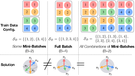
The primary contributions of this paper are twofold. First, we show that under certain parameter settings, mini-batch optimization is equivalent to full-batch optimization if and only if all (NB)\binom{N}{B} mini-batches are selected. These results are based on an interesting connection between contrastive learning and the neural collapse phenomenon [36]. From a computational complexity perspective, the identified equivalence condition may be seen as somewhat prohibitive, as it implies that all (NB)=𝒪(NB)\binom{N}{B}=\mathcal{O}(N^{B}) mini-batches must be considered.

Our second contribution is to show that Ordered SGD (OSGD) [29] can be effective in finding mini-batches that contain the most informative pairs and thereby speeding up convergence. OSGD, proposed in a work by Kawaguchi & Lu [29], is a variant of SGD that modifies the model parameter updates. Instead of using the gradient of the average loss of all samples in a mini-batch, it uses the gradient of the average loss over the top-qq samples in terms of individual loss values. We show that the convergence result from Kawaguchi & Lu [29] can be applied directly to contrastive learning. We also show that OSGD can improve the convergence rate of SGD by a constant factor in certain scenarios. Furthermore, in a novel approach to address the challenge of applying OSGD to the (NB){\binom{N}{B}} mini-batch optimization (which involves examining 𝒪(NB)\mathcal{O}(N^{B}) batches to select high-loss ones), we reinterpret the batch selection as a min-cut problem in graph theory [13]. This novel interpretation allows us to select high-loss batches efficiently via a spectral clustering algorithm [43]. The following informal theorems summarize our main findings.

Theorem 1 (informal).

Under certain parameter settings, the mini-batch optimization of contrastive loss is equivalent to full-batch optimization of contrastive loss if and only if all (NB)\binom{N}{B} mini-batches are selected. Although (NB)\binom{N}{B} mini-batch contrastive loss and full-batch loss are neither identical nor differ by a constant factor, the optimal solutions for both mini-batch and full-batch are identical (see Sec. 4).

Theorem 2 (informal).

In a demonstrative toy example, OSGD operating on the principle of selecting high-loss batches, can potentially converge to the optimal solution of mini-batch contrastive loss optimization faster by a constant factor compared to SGD (see Sec. 5.1).

We validate our theoretical findings and the efficacy of the proposed spectral clustering-based batch selection method by conducting experiments on both synthetic and real data. On synthetic data, we show that our proposed batch-selection algorithms do indeed converge to the optimal solution of full-batch optimization significantly faster than the baselines. We also apply our proposed method to ResNet pre-training with CIFAR-100 [31] and Tiny ImageNet [33]. We evaluate the performance on downstream retrieval tasks, demonstrating that our batch selection method outperforms vanilla SGD in practically relevant settings.

2 Related Work

Contrastive losses.

Contrastive learning has been used for several decades to learn a similarity metric to be used later for applications such as object detection and recognition [41, 1]. Chopra et al. [12] proposed one of the early versions of contrastive loss which has been updated and improved over the years [60, 61, 59, 30, 45]. More recently, contrastive learning has been shown to rival and even surpass traditional supervised learning methods, particularly on image classification tasks [10, 3]. Further, its multi-modal adaptation leverages vast unstructured data, extending its effectiveness beyond image and text modalities [48, 27, 47, 39, 56, 16, 18, 34, 51, 52]. Unfortunately, these methods require extremely large batch sizes in order to perform effectively. Follow-up works showed that using momentum or carefully modifying the augmentation schemes can alleviate this issue to some extent [22, 10, 19, 64].

Effect of batch size.

While most successful applications of contrastive learning use large batch sizes (e.g., 32,768 for CLIP and 8,192 for SimCLR), recent efforts have focused on reducing batch sizes and improving convergence rates [65, 7]. Yuan et al. [68] carefully study the effect of the requirements on the convergence rate when a model is trained for minimizing SimCLR loss, and prove that the gradient of the solution is bounded by 𝒪(1B)\mathcal{O}(\frac{1}{\sqrt{B}}). They also propose SogCLR, an algorithm with a modified gradient update where the correction term allows for an improved convergence rate with better dependence on BB. It is shown that the performance for small batch size can be improved with the technique called hard negative mining [55, 28, 70].

Neural collapse.

Neural collapse is a phenomenon observed in [46] where the final classification layer of deep neural nets collapses to the simplex Equiangular Tight Frame (ETF) when trained well past the point of zero training error [26, 71]. Lu & Steinerberger [36] prove that this occurs when minimizing cross-entropy loss over the unit ball. We extend their proof techniques and show that the optimal solution for minimizing contrastive loss under certain conditions is also the simplex ETF.

Optimal permutations for SGD.

The performance of SGD without replacement under different permutations of samples has been well studied in the literature [5, 53, 54, 42, 66, 2, 49, 40, 58, 57, 20, 44, 37, 50, 63, 38, 6, 11]. One can view batch selection in contrastive learning as a method to choose a specific permutation among the possible (NB)\binom{N}{B} mini-batches of size BB. However, it is important to note that these bounds do not indicate an improved convergence rate for general non-convex functions and thus would not apply to the contrastive loss, particularly in the setting where the embeddings come from a shared embedding network. We show that in the case of OSGD [29], we can indeed prove that contrastive loss satisfies the necessary conditions in order to guarantee convergence.

3 Problem Setting

Suppose we are given a dataset {(𝒙i,𝒚i)}i=1N\{({\bm{x}}_{i},{\bm{y}}_{i})\}_{i=1}^{N} of NN positive pairs (data sample pairs that are conceptually similar or related), where 𝒙i{\bm{x}}_{i} and 𝒚i{\bm{y}}_{i} are two different views of the same object. Note that this setup includes both the multi-modal setting (e.g., CLIP [48]) and the uni-modal setting (e.g., SimCLR [9]) as follows. For the multi-modal case, one can view (𝒙i,𝒚i)({\bm{x}}_{i},{\bm{y}}_{i}) as two different modalities of the same data, e.g., 𝒙i{\bm{x}}_{i} is the image of a scene while 𝒚i{\bm{y}}_{i} is the text description of the scene. For the uni-modal case, one can consider 𝒙i{\bm{x}}_{i} and 𝒚i{\bm{y}}_{i} as different augmented images from the same image.

We consider the contrastive learning problem where the goal is to find embedding vectors for {𝒙i}i=1N\{{\bm{x}}_{i}\}_{i=1}^{N} and {𝒚i}i=1N\{{\bm{y}}_{i}\}_{i=1}^{N}, such that the embedding vectors of positive pairs (𝒙i,𝒚i)({\bm{x}}_{i},{\bm{y}}_{i}) are similar, while ensuring that the embedding vectors of other (negative) pairs are well separated. Let 𝒖id{\bm{u}}_{i}\in{\mathbb{R}}^{d} be the embedding vector of 𝒙i{\bm{x}}_{i}, and 𝒗id{\bm{v}}_{i}\in{\mathbb{R}}^{d} be the embedding vector of 𝒚i{\bm{y}}_{i}. In practical settings, one typically considers parameterized encoders so that 𝒖i=f𝜽(𝒙i){\bm{u}}_{i}=f_{{\bm{\theta}}}({\bm{x}}_{i}) and 𝒗i=gϕ(𝒚i){\bm{v}}_{i}=g_{{\bm{\phi}}}({\bm{y}}_{i}). We define embedding matrices 𝑼:=[𝒖1,𝒖2,𝒖N]{\bm{U}}:=[{\bm{u}}_{1},{\bm{u}}_{2},\ldots{\bm{u}}_{N}] and 𝑽:=[𝒗1,𝒗2,,𝒗N]{\bm{V}}:=[{\bm{v}}_{1},{\bm{v}}_{2},\ldots,{\bm{v}}_{N}] which are the collections of embedding vectors. Now, we focus on the simpler setting of directly optimizing the embedding vectors instead of model parameters 𝜽{\bm{\theta}} and ϕ{\bm{\phi}} in order to gain theoretical insights into the learning embeddings. This approach enables us to develop a deeper understanding of the underlying principles and mechanisms. Consider the problem of directly optimizing the embedding vectors for NN pairs which is given by

min𝑼,𝑽con(𝑼,𝑽)s.t.𝒖i=1,𝒗i=1i[N],\min_{{\bm{U}},{\bm{V}}}\ {\mathcal{L}}^{\operatorname{con}}({\bm{U}},{\bm{V}})\quad\text{s.t.}\quad\lVert{\bm{u}}_{i}\rVert=1,\lVert{\bm{v}}_{i}\rVert=1\;\quad\forall i\in[N], (1)

where \lVert\cdot\rVert denotes the 2\ell_{2} norm, the set [N][N] denotes the set of integers from 11 to NN, and the contrastive loss (the standard InfoNCE loss [45]) is defined as

con(𝑼,𝑽):=1Ni=1Nlog(e𝒖i𝒗ij=1Ne𝒖i𝒗j)1Ni=1Nlog(e𝒗i𝒖ij=1Ne𝒗i𝒖j).\displaystyle{\mathcal{L}}^{\operatorname{con}}({\bm{U}},{\bm{V}}):=-\frac{1}{N}\sum_{i=1}^{N}\log\left(\frac{e^{{\bm{u}}_{i}^{\intercal}{\bm{v}}_{i}}}{\sum_{j=1}^{N}e^{{{\bm{u}}}_{i}^{\intercal}{{\bm{v}}}_{j}}}\right)-\frac{1}{N}\sum_{i=1}^{N}\log\left(\frac{e^{{\bm{v}}_{i}^{\intercal}{\bm{u}}_{i}}}{\sum_{j=1}^{N}e^{{{\bm{v}}}_{i}^{\intercal}{{\bm{u}}}_{j}}}\right). (2)

Note that con(𝑼,𝑽){\mathcal{L}}^{\operatorname{con}}({\bm{U}},{\bm{V}}) is the full-batch version of the loss which contrasts all embeddings with each other. However, due to the large computational complexity and memory requirements during optimization, practitioners often consider the following mini-batch version instead. Note that there exist (NB)\binom{N}{B} different mini-batches, each of which having BB samples. For k[(NB)]k\in\left[\binom{N}{B}\right], let k{\mathcal{B}}_{k} be the kk-th mini-batch satisfying k[N]{\mathcal{B}}_{k}\subset[N] and |k|=B|{\mathcal{B}}_{k}|=B. Let 𝑼k:={𝒖i}ik{\bm{U}}_{{\mathcal{B}}_{k}}:=\{{\bm{u}}_{i}\}_{i\in{\mathcal{B}}_{k}} and 𝑽k:={𝒗i}ik{\bm{V}}_{{\mathcal{B}}_{k}}:=\{{\bm{v}}_{i}\}_{i\in{\mathcal{B}}_{k}}. Then, the contrastive loss for the kk-th mini-batch is con(𝑼k,𝑽k){\mathcal{L}}^{\operatorname{con}}({\bm{U}}_{{\mathcal{B}}_{k}},{\bm{V}}_{{\mathcal{B}}_{k}}).

4 Relationship Between the Optimization for Full-Batch and Mini-Batch

Recall that we focus on finding the optimal embedding matrices (𝑼{\bm{U}}, 𝑽{\bm{V}}) that minimize the contrastive loss. In this section, we investigate the relationship between the problem of optimizing the full-batch loss con(𝑼,𝑽){\mathcal{L}}^{\operatorname{con}}({\bm{U}},{\bm{V}}) and the problem of optimizing the mini-batch loss con(𝑼k,𝑽k){\mathcal{L}}^{\operatorname{con}}({\bm{U}}_{{\mathcal{B}}_{k}},{\bm{V}}_{{\mathcal{B}}_{k}}). Towards this goal, we prove three main results, the proof of which are in Appendix B.1.

  • We derive the optimal solution that minimizes the full-batch loss (Lem. 1, Thm. 3).

  • We show that the solution that minimizes the average of (NB)\binom{N}{B} mini-batch losses is identical to the one that minimizes the full-batch loss (Prop. 1, Thm. 4).

  • We show that minimizing the mini-batch loss summed over only a strict subset of (NB)\binom{N}{B} mini-batches can lead to a sub-optimal solution that does not minimize the full-batch loss (Thm. 5).

4.1 Full-batch Contrastive Loss Optimzation

In this section, we characterize the optimal solution for the full-batch loss minimization in Eq. (1). We start by providing the definition of the simplex equiangular tight frame (ETF) which turns out to be the optimal solution in certain cases. The original definition of ETF [62] is for NN vectors in a dd-dimensional space where Nd+1N\geq d+1 111See Def. 4 in Appendix A for the full definition. Papyan et al. [46] defines the ETF for the case where Nd+1N\leq d+1 to characterize the phenomenon of neural collapse. In our work, we use the latter definition of simplex ETFs which is stated below.

Definition 1 (Simplex ETF).

We call a set of NN vectors {𝒖i}i=1N\{{\bm{u}}_{i}\}_{i=1}^{N} form a simplex Equiangular Tight Frame (ETF) if 𝒖i=1,i[N]\lVert{\bm{u}}_{i}\rVert=1,\forall i\in[N] and 𝒖i𝒖j=1/(N1),ij{\bm{u}}_{i}^{\intercal}{\bm{u}}_{j}=-1/(N-1),\forall i\neq j.

In the following Lemma, we first prove that the optimal solution of full-batch contrastive learning is the simplex ETF for Nd+1N\leq d+1 which follows almost directly from Lu & Steinerberger [36].

Lemma 1 (Optimal solution when Nd+1N\leq d+1).

Suppose Nd+1N\leq d+1. Then, the optimal solution (𝐔,𝐕)({\bm{U}}^{\star},{\bm{V}}^{\star}) of the full-batch contrastive learning problem in Eq. (1) satisfies two properties: (i) 𝐔=𝐕{\bm{U}}^{\star}={\bm{V}}^{\star}, and (ii) the columns of 𝐔{\bm{U}}^{\star} form a simplex ETF.

Actually, many practical scenarios satisfy N>d+1N>d+1. However, the approach used in Lu & Steinerberger [36] cannot be directly applied for N>d+1N>d+1, leaving it as an open problem. While solving the open problem for the general case seems difficult, we characterize the optimal solution for the specific case of N=2dN=2d, subject to the conditions stated below.

Definition 2 (Symmetric and Antipodal).

Embedding matrices 𝑼{\bm{U}} and 𝑽{\bm{V}} are called symmetric and antipodal if (𝑼,𝑽)({\bm{U}},{\bm{V}}) satisfies two properties: (i) Symmetric i.e., 𝑼=𝑽{\bm{U}}={\bm{V}}; (ii) Antipodal i.e., for each i[N]i\in[N], there exists j(i)j(i) such that 𝒖j(i)=𝒖i{\bm{u}}_{j(i)}=-{\bm{u}}_{i}.

We conjecture that the optimal solutions for N=2dN=2d are symmetric and antipodal. Note that the symmetric property holds for Nd+1N\leq d+1 case, and the antipodality is frequently assumed in geometric problems such as the sphere covering problem in [4].

Thm. 3 shows that when N=2dN=2d, the optimal solution for the full-batch loss minimization, under a symmetric and antipodal configuration, form a cross-polytope which is defined as the following.

Definition 3 (Simplex cross-polytope).

We call a set of NN vectors {𝒖}i=1N\{{\bm{u}}\}_{i=1}^{N} form a simplex cross-polytope if, for all ii, the following three conditions hold: 𝒖i=1\|{\bm{u}}_{i}\|=1; there exists a unique jj such that 𝒖i𝒖j=1{\bm{u}}_{i}^{\intercal}{\bm{u}}_{j}=-1; and 𝒖i𝒖k=0{\bm{u}}_{i}^{\intercal}{\bm{u}}_{k}=0 for all k{i,j}k\notin\{i,j\}.

Theorem 3 (Optimal solution when N=2dN=2d).

Let

(𝑼,𝑽):=argmin(𝑼,𝑽)𝒜con(𝑼,𝑽)s.t.𝒖i=1,𝒗i=1i[N],\displaystyle({\bm{U}}^{\star},{\bm{V}}^{\star}):=\arg\min_{({\bm{U}},{\bm{V}})\in{\mathcal{A}}}{\mathcal{L}}^{\operatorname{con}}({\bm{U}},{\bm{V}})\quad\text{s.t.}\quad\|{\bm{u}}_{i}\|=1,\|{\bm{v}}_{i}\|=1\quad\forall i\in[N], (3)

where 𝒜:={(𝐔,𝐕):𝐔,𝐕 are symmetric and antipodal}{\mathcal{A}}:=\{({\bm{U}},{\bm{V}}):{\bm{U}},{\bm{V}}\text{ are symmetric and antipodal}\}. Then, the columns of 𝐔{\bm{U}}^{\star} form a simplex cross-polytope for N=2dN=2d.

Proof Outline. By the antipodality assumption, we can apply Jensen’s inequality to N2N-2 indices without itself 𝒖i{{\bm{u}}}_{i} and antipodal point 𝒖i-{\bm{u}}_{i} for a given i[N]i\in[N]. Then we show that the simplex cross-polytope also minimizes this lower bound while satisfying the conditions that make the applications of Jensen’s inequality tight.

For the general case of N>d+1N>d+1, excluding N=2d,N=2d, we still leave it as an open problem.

4.2 Mini-batch Contrastive Loss Optimization

Refer to caption
Refer to caption
Figure 1: (a) Comparing mini-batch loss and full-batch loss when N=10,B=2N=10,B=2, and d=2d=2. We illustrate this by manipulating a single embedding vector 𝒖1{\bm{u}}_{1} while maintaining all other embeddings (𝒗1{\bm{v}}_{1} and {𝒖i,𝒗i}i=210\{{\bm{u}}_{i},{\bm{v}}_{i}\}_{i=2}^{10}) at their optimal solutions. Specifically, 𝒖1=[u1,1,u1,2]{\bm{u}}_{1}=[u_{1,1},u_{1,2}] is varied as [cos(θ),sin(θ)][\cos(\theta),\sin(\theta)] for θ[π,π]\theta\in[-\pi,\pi]. While the two loss functions are not identical, corroborating Prop.1, their minimizers align, providing empirical support for Thm. 4; (b) The relationship between full-batch and mini-batch optimization in contrastive learning. Consider optimizing N=4N=4 pairs of d=3d=3 dimensional embedding vectors {(𝒖i,𝒗i)}i=1N\{({\bm{u}}_{i},{\bm{v}}_{i})\}_{i=1}^{N} where 𝒖i{\bm{u}}_{i} and 𝒗i{\bm{v}}_{i} are shown as colored square and circle, respectively. The index ii is written in the square/circle. The black rounded box represents a batch. We compare three batch selection options: (i) full batch, i.e., B=4B=4, (ii) all (NB)=6\binom{N}{B}=6 mini-batches with size B=2B=2, and (iii) some mini-batches. Here, 𝒮B{\mathcal{S}}_{B} is the set of mini-batches where each mini-batch is represented by the set of constituent samples’ indices. Our theoretical/empirical findings are: the optimal embedding that minimizes full-batch loss and the one that minimizes the sum of (NB)\binom{N}{B} mini-batch losses are identical, while the one that minimizes the mini-batch losses summed over only a strict subset of (NB)\binom{N}{B} batches does not guarantee the negative correlation between 𝒖i{\bm{u}}_{i} and 𝒖j{\bm{u}}_{j} for iji\neq j. This illustration is supported by our mathematical results in Thms. 4 and  5.

Here we consider the mini-batch contrastive loss optimization problem, where we first choose multiple mini-batches of size BB and then find 𝑼,𝑽{\bm{U}},{\bm{V}} that minimize the sum of contrastive losses computed for the chosen mini-batches. Note that this is the loss that is typically considered in the contrastive learning since computing the full-batch loss is intractable in practice. Let us consider a subset of all possible (NB)\binom{N}{B} mini-batches and denote their indices by 𝒮B[(NB)]{\mathcal{S}}_{B}\subseteq\left[\binom{N}{B}\right]. For a fixed 𝒮B{\mathcal{S}}_{B}, the mini-batch loss optimization problem is formulated as:

min𝑼,𝑽minicon(𝑼,𝑽;𝒮B)s.t.𝒖i=1,𝒗i=1i[N],\min_{{\bm{U}},{\bm{V}}}\ {\mathcal{L}}^{\operatorname{con}}_{\operatorname{mini}}({\bm{U}},{\bm{V}};{\mathcal{S}}_{B})\quad\text{s.t.}\quad\lVert{\bm{u}}_{i}\rVert=1,\lVert{\bm{v}}_{i}\rVert=1\;\quad\forall i\in[N], (4)

where the loss of given mini-batches is minicon(𝑼,𝑽;𝒮B):=1|𝒮B|i𝒮Bcon(𝑼i,𝑽i).{\mathcal{L}}^{\operatorname{con}}_{\operatorname{mini}}({\bm{U}},{\bm{V}};{\mathcal{S}}_{B}):=\frac{1}{|{\mathcal{S}}_{B}|}\sum_{i\in{\mathcal{S}}_{B}}{\mathcal{L}}^{\operatorname{con}}({\bm{U}}_{{\mathcal{B}}_{i}},{\bm{V}}_{{\mathcal{B}}_{i}}). To analyze the relationship between the full-batch loss minimization in Eq. (1) and the mini-batch loss minimization in Eq. (4), we first compare the objective functions of two problems as below.

Proposition 1.

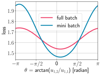
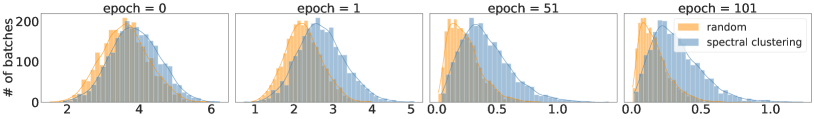
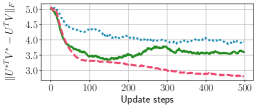
The mini-batch loss and full-batch loss are not identical, nor is one a simple scaling of the other by a constant factor. In other words, when 𝒮B=[(NB)]{\mathcal{S}}_{B}=\left[\binom{N}{B}\right], for all B2B\geq 2, there exists no constant cc such that minicon(𝐔,𝐕;𝒮B)=ccon(𝐔,𝐕)for all𝐔,𝐕{\mathcal{L}}^{\operatorname{con}}_{\operatorname{mini}}({\bm{U}},{\bm{V}};{\mathcal{S}}_{B})=c\cdot{\mathcal{L}}^{\operatorname{con}}({\bm{U}},{\bm{V}})\quad\text{for all}\quad{\bm{U}},{\bm{V}}.

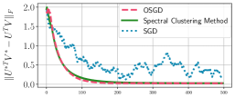
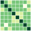
We illustrate this proposition by visualizing the two loss functions in Fig. 1 when N=10,B=2N=10,B=2, and d=2d=2. We visualize it along a single embedding vector 𝒖1{\bm{u}}_{1} by freezing all other embeddings (𝒗1{\bm{v}}_{1} and {𝒖i,𝒗i}i=210\{{\bm{u}}_{i},{\bm{v}}_{i}\}_{i=2}^{10}) at the optimal solution and varying 𝒖1=[u1,1,u1,2]{\bm{u}}_{1}=[u_{1,1},u_{1,2}] as [cos(θ),sin(θ)][\cos(\theta),\sin(\theta)] for θ[π,π]\theta\in[-\pi,\pi]. One can confirm that two losses are not identical (even up to scaling).

Interestingly, the following result shows that the optimal solutions of both problems are identical.

Theorem 4 (Optimization with all possible (NB){\binom{N}{B}} mini-batches).

Suppose B2B\geq 2. The set of minimizers of the (NB)\binom{N}{B} mini-batch problem in Eq. (4) is the same as that of the full-batch problem in Eq. (1) for two cases: (i) Nd+1N\leq d+1, and (ii) N=2dN=2d and the pairs (𝐔{\bm{U}}, 𝐕{\bm{V}}) are restricted to those satisfying the conditions stated in Def. 2. In such cases, the solutions (𝐔,𝐕)({\bm{U}},{\bm{V}}) for the (NB)N\choose B mini-batch optimization problem satisfies the following: Case (i) {𝐮i}i=1N\{{{\bm{u}}_{i}}\}_{i=1}^{N} forms a simplex ETF and 𝐮i=𝐯i{{\bm{u}}}_{i}={{\bm{v}}}_{i} for all i[N]i\in[N]; Case (ii): {𝐮i}i=1N\{{{\bm{u}}_{i}}\}_{i=1}^{N} forms a simplex cross-polytope.

Proof Outline. Similar to the proof of Lem. 1, we bound the objective function from below using Jensen’s inequality. Then, we show that this lower bound is equivalent to a scaling of the bound from the proof of Lem. 1, by using careful counting arguments. Then, we can simply repeat the rest of the proof to show that the simplex ETF also minimizes this lower bound while satisfying the conditions that make the applications of Jensen’s inequality tight.

Now, we present mathematical results specifying the cases when the solutions of mini-batch optimization and full-batch optimization differ. First, we show that when B=2B=2, minimizing the mini-batch loss over any strict subset of (NB)\binom{N}{B} batches, is not equivalent to minimizing the full-batch loss.

Theorem 5 (Optimization with fewer than (NB){\binom{N}{B}} mini-batches).

Suppose B=2B=2 and Nd+1N\leq d+1. Then, the minimizer of Eq. (4) for 𝒮B[(NB)]{\mathcal{S}}_{B}\subsetneq\left[{\binom{N}{B}}\right] is not the minimizer of the full-batch optimization in Eq. (1).

Proof Outline. We show that there exist embedding vectors that are not the simplex ETF, and have a strictly lower objective value. This implies that the optimal solution of any set of mini-batches that does not contain all (N2)\binom{N}{2} mini-batches is not the same as that of the full-batch problem.

The result of Thm. 5 is extended to the general case of B2B\geq 2, under some mild assumption; please check Prop. 2 and 3 in Appendix B.1. Fig. 1 summarizes the main findings in this section.

5 Ordered Stochastic Gradient Descent for Mini-Batch Contrastive Learning

Recall that the optimal embeddings for the full-batch optimization problem in Eq. (1) can be obtained by minimizing the sum of (NB)\binom{N}{B} mini-batch losses, according to Thm. 4. An easy way of approximating the optimal embeddings is using gradient descent (GD) on the sum of losses for (NB)\binom{N}{B} mini-batches, or to use a stochastic approach which applies GD on the loss for a randomly chosen mini-batch. Recent works found that applying GD on selective batches outperforms SGD in some cases [29, 37, 35]. A natural question arises: does this hold for mini-batch contrastive learning? Specifically, (i) Is SGD enough to guarantee good convergence on mini-batch contrastive learning?, and (ii) Can we come up with a batch selection method that outperforms vanilla SGD? To answer this question:

  • We show that Ordered SGD (OSGD) [29] can potentially accelerate convergence compared to vanilla SGD in a demonstrative toy example (Sec. 5.1). We also show that the convergence results from Kawaguchi & Lu [29] can be extended to mini-batch contrastive loss optimization (Sec. 5.2).

  • We reformulate the batch selection problem into a min-cut problem in graph theory [13], by considering a graph with NN nodes where each node is each positive pair and each edge represents a proxy to the contrastive loss between two nodes. This allows us to devise an efficient batch selection algorithm by leveraging spectral clustering [43] (Sec. 5.3).

5.1 Convergence Comparison in a Toy Example: OSGD vs. SGD

This section investigates the convergence of two gradient-descent-based methods, OSGD and SGD. The below lemma shows that the contrastive loss is geodesic non-quasi-convex, which implies the hardness of proving the convergence of gradient-based methods for contrastive learning in Eq. (1).

Lemma 2.

Contrastive loss con(𝐔,𝐕){\mathcal{L}}^{\operatorname{con}}({\bm{U}},{\bm{V}}) is a geodesic non-quasi-convex function of 𝐔,𝐕{\bm{U}},{\bm{V}} on 𝒯={(𝐔,𝐕):𝐮i=𝐯i=1,i[N]}{\mathcal{T}}=\{({\bm{U}},{\bm{V}}):\lVert{\bm{u}}_{i}\rVert=\lVert{\bm{v}}_{i}\rVert=1,\forall i\in[N]\}.

We provide the proof in Appendix B.2.

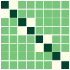
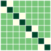
In order to compare the convergence of OSGD and SGD, we focus on a toy example where convergence to the optimal solution is achievable with appropriate initialization. Consider a scenario where we have N=4N=4 embedding vectors {𝒖i}i=1N\{{\bm{u}}_{i}\}_{i=1}^{N} with 𝒖i2{\bm{u}}_{i}\in{\mathbb{R}}^{2}. Each embedding vector is defined as 𝒖1=(cosθ1,sinθ1);𝒖2=(cosθ2,sinθ2);𝒖3=(cosθ3,sinθ3);𝒖4=(cosθ4,sinθ4){\bm{u}}_{1}=(\cos\theta_{1},\sin\theta_{1});{\bm{u}}_{2}=(\cos\theta_{2},-\sin\theta_{2});{\bm{u}}_{3}=(-\cos\theta_{3},-\sin\theta_{3});{\bm{u}}_{4}=(-\cos\theta_{4},\sin\theta_{4}) for parameters {θi}i=1n\{\theta_{i}\}_{i=1}^{n}. Over time step tt, we consider updating the parameters 𝜽(t):=[θ1(t),θ2(t),θ3(t),θ4(t)]{\bm{\theta}}^{(t)}:=[\theta_{1}^{(t)},\theta_{2}^{(t)},\theta_{3}^{(t)},\theta_{4}^{(t)}] using gradient descent based methods. For all ii, the initial parameters are set as θi(0)=ϵ>0\theta_{i}^{(0)}=\epsilon>0, and the other embedding vectors are initialized as 𝒗i(0)=𝒖i(0){\bm{v}}_{i}^{(0)}={\bm{u}}_{i}^{(0)}. This setting is illustrated in Fig. 2.

Refer to caption
Refer to caption
Figure 2: (a) Toy example considered in Sec. 5.1; (b) The training loss curves of three algorithms (OSGD, SGD, and (NB)\binom{N}{B} full-batch gradient descent) applied on the toy example when N=4N=4 and B=2B=2. The x-axis represents the number of update steps, while the y-axis displays the loss in Eq. (2). OSGD converges the fastest among the three methods.

At each time step tt, each learning algorithm begins by selecting a mini-batch (t){1,2,3,4}{\mathcal{B}}^{(t)}\subset\left\{1,2,3,4\right\} with batch size |(t)|=2|{\mathcal{B}}^{(t)}|=2. SGD randomly selects a mini-batch, while OSGD selects a mini-batch as follows: (t)=argmax𝒮con(𝑼(𝜽(t)),𝑽(𝜽(t))){\mathcal{B}}^{(t)}=\arg\max\limits_{{\mathcal{B}}\in{\mathcal{S}}}{\mathcal{L}}^{\operatorname{con}}({\bm{U}}_{{\mathcal{B}}}({\bm{\theta}}^{(t)}),{\bm{V}}_{{\mathcal{B}}}({\bm{\theta}}^{(t)})). Then, the algorithms update 𝜽(t){\bm{\theta}}^{(t)} using gradient descent on con(𝑼,𝑽){\mathcal{L}}^{\operatorname{con}}({\bm{U}}_{{\mathcal{B}}},{\bm{V}}_{{\mathcal{B}}}) with a learning rate η\eta: 𝜽(t+1)=𝜽(t)η𝜽con(𝑼(t),𝑽(t)){\bm{\theta}}^{(t+1)}={\bm{\theta}}^{(t)}-\eta\nabla_{{\bm{\theta}}}{\mathcal{L}}^{\operatorname{con}}({\bm{U}}_{{\mathcal{B}}^{(t)}},{\bm{V}}_{{\mathcal{B}}^{(t)}}). For a sufficiently small margin ρ>0\rho>0, let TOSGD,TSGDT_{\textnormal{OSGD}},T_{\textnormal{SGD}} be the minimal time required for the algorithms to reach the condition 𝔼[𝜽(T)](π/4ρ,π/4)N\mathbb{E}[{\bm{\theta}}^{(T)}]\in(\pi/4-\rho,\pi/4)^{N}. Under this setting, the following theorem compares OSGD and SGD, in terms of the lower bound on the time required for the convergence to the optimal solution.

Theorem 6.

Consider the described setting where the parameters 𝛉(t){\bm{\theta}}^{(t)} of embedding vectors are updated, as shown in Fig. 2. Suppose there exist ϵ~\tilde{\epsilon}, T¯\overline{T} such that for all tt satisfying (t)={1,3}{\mathcal{B}}^{(t)}=\left\{1,3\right\} or {2,4}\left\{2,4\right\}, 𝛉(t)con(𝐔(t),𝐕(t))ϵ~\|\nabla_{{\bm{\theta}}^{(t)}}{\mathcal{L}}^{\operatorname{con}}({\bm{U}}_{{\mathcal{B}}^{(t)}},{\bm{V}}_{{\mathcal{B}}^{(t)}})\|\leq\tilde{\epsilon}, and TOSGD,TSGD<T¯.T_{\textnormal{OSGD}},\ T_{\textnormal{SGD}}<\overline{T}. Then, we have the following inequalities:

TOSGDπ/4ρϵ+O(η2ϵ+ηϵ3)ηϵ,TSGD3(e2+1)e21π/4ρϵ+O(η2ϵ+η2ϵ~)ηϵ+O(ηϵ3+ηϵ~).T_{\textnormal{OSGD}}\geq{\pi/4-\rho-\epsilon+O(\eta^{2}\epsilon+\eta\epsilon^{3})\over\eta\epsilon},\quad T_{\textnormal{SGD}}\geq{3(e^{2}+1)\over e^{2}-1}{\pi/4-\rho-\epsilon+O(\eta^{2}\epsilon+\eta^{2}\tilde{\epsilon})\over\eta\epsilon+O(\eta\epsilon^{3}+\eta\tilde{\epsilon})}.
Corollary 1.

Suppose lower bounds of TOSGDT_{\textnormal{OSGD}}, TSGDT_{\textnormal{SGD}} in Thm. 6 are tight, and the learning rate η\eta is small enough. Then, TOSGD/TSGD=(e21)/3(e2+1)1/4T_{\textnormal{OSGD}}/T_{\textnormal{SGD}}=(e^{2}-1)/3(e^{2}+1)\approx 1/4.

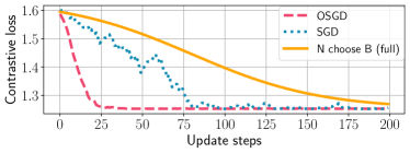
In Fig. 2, we present training loss curves of the full-batch contrastive loss in Eq. (2) for various algorithms implemented on the toy example. One can observe that the losses of all algorithms eventually converge to 1.253, the optimal loss achievable when the solution satisfies 𝒖i=𝒗i{\bm{u}}_{i}={\bm{v}}_{i} and {𝒖i}i=1N\{{\bm{u}}_{i}\}_{i=1}^{N} form simplex cross-polytope. As shown in the figure, OSGD converges faster than SGD to the optimal loss. This empirical evidence corroborates our theoretical findings in Corollary 1.

5.2 Convergence of OSGD in Mini-batch Contrastive Learning Setting

Recall that it is challenging to prove the convergence of gradient-descent-based methods for contrastive learning problem in Eq. (1) due to the non-quasi-convexity of the contrastive loss con\mathcal{L}^{\text{con}}. Instead of focusing on the contrastive loss, we consider a proxy, the weighted contrastive loss defined as ~con(𝑼,𝑽)1qj=1(NB)γjcon(𝑼(j),𝑽(j))\widetilde{{\mathcal{L}}}^{\operatorname{con}}({\bm{U}},{\bm{V}})\coloneqq\frac{1}{q}\sum_{j=1}^{{N\choose B}}\gamma_{j}{\mathcal{L}}^{\operatorname{con}}({\bm{U}}_{{\mathcal{B}}_{(j)}},{\bm{V}}_{{\mathcal{B}}_{(j)}}) with γj=l=0q1(j1l)((NB)jkl1)/((NB)k)\gamma_{j}={\sum_{l=0}^{q-1}{j-1\choose l}{{N\choose B}-j\choose k-l-1}}/{{{N\choose B}\choose k}} for two arbitrary natural numbers k,q(NB)k,q\leq\binom{N}{B} where (j){\mathcal{B}}_{(j)} is a mini-batch with jj-th largest loss among batches of size BB. Indeed, this is a natural objective obtained by applying OSGD to our problem, and we show the convergence of such an algorithm by extending the results in Kawaguchi & Lu [29]. OSGD updates the embedding vectors using the gradient averaged over qq batches that have the largest losses among randomly chosen kk batches (see Algo. 2 in Appendix B.2). Let 𝑼(t){\bm{U}}^{(t)}, 𝑽(t){\bm{V}}^{(t)} be the updated embedding matrices when applying OSGD for tt steps starting from 𝑼(0){\bm{U}}^{(0)}, 𝑽(0){\bm{V}}^{(0)}, using the learning rate ηt\eta_{t}. Then the following theorem, proven in Appendix B.2, holds.

Theorem 7 (Convergence results).

Consider sampling tt^{\star} from [T1][T-1] with probability proportional to {ηt}t=0T1\{\eta_{t}\}_{t=0}^{T-1}, that is, (t=t)=ηt/(i=0T1ηi){\mathbb{P}}(t^{\star}=t)={\eta_{t}}/{(\sum_{i=0}^{T-1}\eta_{i})}. Then ρ>ρ0=22/B+4e2/B\forall\rho>\rho_{0}=2\sqrt{2/B}+4e^{2}/B, we have

𝔼[~con(𝑼(t),𝑽(t))2](ρ+ρ0)2ρ(ρρ0)(~con(𝑼(0),𝑽(0))~con)+8ρt=0T1ηt2t=0T1ηt,{\mathbb{E}}\left[\left\|\nabla\widetilde{{\mathcal{L}}}^{\operatorname{con}}({\bm{U}}^{(t^{\star})},{\bm{V}}^{(t^{\star})})\right\|^{2}\right]\leq\frac{(\rho+\rho_{0})^{2}}{\rho(\rho-\rho_{0})}\frac{\left(\widetilde{{\mathcal{L}}}^{\operatorname{con}}({\bm{U}}^{(0)},{\bm{V}}^{(0)})-\widetilde{{\mathcal{L}}}^{\operatorname{con}\star}\right)+8{\rho}\sum_{t=0}^{T-1}\eta_{t}^{2}}{\sum_{t=0}^{T-1}\eta_{t}},

where ~con\widetilde{{\mathcal{L}}}^{\operatorname{con}\star} denotes the minimized value of ~con\widetilde{{\mathcal{L}}}^{\operatorname{con}}.

Given sufficiently small learning rate ηtO(t1/2),\eta_{t}\sim O(t^{-1/2}), 𝔼~con2\mathbb{E}\|\nabla\widetilde{{\mathcal{L}}}^{\operatorname{con}}\|^{2} decays at the rate of O~(T1/2).\widetilde{O}(T^{-1/2}). Therefore, this theorem guarantees the convergence of OSGD for mini-batch contrastive learning.

5.3 Suggestion: Spectral Clustering-based Approach

Refer to caption
Figure 3: Histograms of batch counts for N/BN/B batches, for the contrastive loss measured from ResNet-18 models trained on CIFAR-100 using SGD, where NN=50,000 and BB=20. Each plot is derived from a distinct training epoch. Here we compare two batch selection methods: (i) randomly shuffling NN samples and partition them into N/BN/B batches of size BB, (ii) our SC method given in Algo. 1. The histograms show that batches generated through the proposed spectral clustering method tend to contain a higher proportion of large loss values when compared to random batch selection. Similar results are observed in different settings, details of which are given in Appendix D.1.
Input: the number of positive pairs NN, batch size BB, embedding matrices: 𝑼{\bm{U}}, 𝑽{\bm{V}}
Output: selected batches {j}j=1N/B\{{\mathcal{B}}_{j}\}_{j=1}^{N/B}
1 Construct the affinity matrix AA: Aij=𝟙{ij}×w(i,j)A_{ij}=\mathbbm{1}\{i\neq j\}\times w(i,j)
2 Construct the degree matrix DD from AA: Dij=𝟙{i=j}×(j=1NAij)D_{ij}=\mathbbm{1}\{i=j\}\times(\sum_{j=1}^{N}A_{ij})
3 LDAL\leftarrow D-A; kN/Bk\leftarrow N/B
4 {j}j=1N/B\{{\mathcal{B}}_{j}\}_{j=1}^{N/B}\leftarrowApply the even-sized spectral clustering algorithm with LL and kk
return {j}j=1N/B\{{\mathcal{B}}_{j}\}_{j=1}^{N/B}
Algorithm 1 Spectral Clustering Method

Applying OSGD to mini-batch contrastive learning has a potential benefit as shown in Sec. 5.1, but it also has some challenges. Choosing the best qq batches with high loss in OSGD is only doable after we evaluate losses of all (NB)\binom{N}{B} combinations, which is computationally infeasible for large NN. A naive solution to tackle this challenge is to first randomly choose kk batches and then select qq high-loss batches among kk batches. However, this naive random batch selection method does not guarantee that the chosen qq batches are having the highest loss among all (NB)\binom{N}{B} candidates. Motivated by these issues of OSGD, we suggest an alternative batch selection method inspired by graph theory. Note that the contrastive loss 𝖼𝗈𝗇(U,V)\mathcal{L}^{\sf{con}}(U_{{\mathcal{B}}},V_{{\mathcal{B}}}) for a given batch {\mathcal{B}} is lower bounded as follows:

1B(B1){ij{i}log(1+(B1)e𝒖i(𝒗j𝒗i))+log(1+(B1)e𝒗i(𝒖j𝒖i))}.\displaystyle\begin{aligned} &\frac{1}{B(B-1)}\left\{\sum_{i\in{\mathcal{B}}}\sum_{j\in{\mathcal{B}}\setminus\{i\}}\log\left(1+(B-1)e^{{\bm{u}}_{i}^{\intercal}({\bm{v}}_{j}-{\bm{v}}_{i})}\right)+\log\left(1+(B-1)e^{{\bm{v}}_{i}^{\intercal}({\bm{u}}_{j}-{\bm{u}}_{i})}\right)\right\}.\end{aligned} (5)

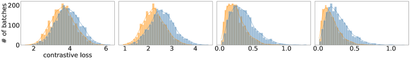
This lower bound is derived using Jensen’s inequality. Detailed derivation is provided in Appendix C.1. A nice property of this lower bound is that it can be expressed as a summation of terms over a pair (i,j)(i,j) of samples within batch {\mathcal{B}}. Consider a graph 𝒢{\mathcal{G}} with NN nodes, where the weight between node kk and ll is defined as w(k,l):=(i,j){(k,l),(l,k)}log(1+(B1)e𝒖i(𝒗j𝒗i))+log(1+(B1)e𝒗i(𝒖j𝒖i))w(k,l):=\sum_{(i,j)\in\{(k,l),(l,k)\}}\log\left(1+(B-1)e^{{\bm{u}}_{i}^{\intercal}({\bm{v}}_{j}-{\bm{v}}_{i})}\right)+\log\left(1+(B-1)e^{{\bm{v}}_{i}^{\intercal}({\bm{u}}_{j}-{\bm{u}}_{i})}\right). Recall that our goal is to choose qq batches having the highest contrastive loss among (NB)N\choose B batches. We relax this problem by reducing our search space such that the q=N/Bq=N/B chosen batches 1,,q{\mathcal{B}}_{1},\cdots,{\mathcal{B}}_{q} form a partition of NN samples, i.e., ij={\mathcal{B}}_{i}\cap{\mathcal{B}}_{j}=\varnothing and i[q]i=[N]\cup_{i\in[q]}{\mathcal{B}}_{i}=[N]. In such scenario, our target problem is equivalent to the problem of clustering NN nodes in graph 𝒢{\mathcal{G}} into qq clusters with equal size, where the objective is to minimize the sum of weights of inter-cluster edges. This problem is nothing but the min-cut problem [13], and we can employ even-sized spectral clustering algorithm which solves it efficiently. The pseudo-code of our batch selection method222Our algorithm finds N/BN/B good clusters at once, instead of only finding a single best cluster. Compared with such alternative approach, our method is (i) more efficient when we update models for multiple iterations, and (ii) guaranteed to load all samples with N/BN/B batches, thus expected to have better convergence [5, 21, 20]. is provided in Algo. 1, and further details of the algorithm are provided in Appendix C. Fig. 3 shows the histogram of contrastive loss for N/BN/B batches chosen by the random batch selection method and the proposed spectral clustering (SC) method. One can observe that the SC method favors batches with larger loss values.

6 Experiments

We validate our theoretical findings and the effectiveness of our proposed batch selection method by providing experimental results on synthetic and real datasets. We first show that our experimental results on synthetic dataset coincide with two main theoretical results: (i) the relationship between the full-batch contrastive loss and the mini-batch contrastive loss given in Sec. 4, (ii) the analysis on the convergence of OSGD and the proposed SC method given in Sec. 5. To demonstrate the practicality of our batch selection method, we provide experimental results on CIFAR-100 [31] and Tiny ImageNet [33]. Details of the experimental setting can be found in Appendix D, and our code is available at https://github.com/krafton-ai/mini-batch-cl.

d=2Nd=2N Refer to captionRefer to captionRefer to captionRefer to captionRefer to caption

d=N/2d=N/2

Refer to caption
(a) optimal
Refer to caption
(b) full-batch
Refer to caption
(c) (NB){N\choose B}-all
Refer to caption
(d) (NB){N\choose B}-sub
Refer to caption
(e) norm difference
Figure 4: The behavior of embedding matrices 𝑼,𝑽{\bm{U}},{\bm{V}} optimized by different batch selection methods for N=8N=8 and B=2B=2 (Top: d=2Nd=2N, Bottom: d=N/2d=N/2). (a)-(d): Heatmap of N×NN\times N matrix visualizing the pairwise inner products 𝒖i𝒗j{\bm{u}}_{i}^{\intercal}{\bm{v}}_{j}, where (a): ground-truth solution (ETF for d=2Nd=2N, cross-polytope for d=N/2d=N/2), (b): optimized the full-batch loss with GD, (c): optimized the sum of (NB)\binom{N}{B} mini-batch losses with GD, (d): optimized a partial sum of (NB)\binom{N}{B} mini-batch losses with GD. Note that both (b) and (c) reach the ground-truth solution in (a), while (d) does not, supporting our theoretical results in Sec. 4.2. Further, (e) compares the convergence of three mini-batch selection algorithms: 1) SGD, 2) OSGD, and 3) our spectral clustering method, when updating embeddings for 500 steps. OSGD and our method nearly converge to the optimal solution, while SGD does not. Here, yy-axis represents the Frobenius norm of the difference between the heatmaps of the optimal solution and the updated embeddings, denoted by 𝑼𝑽𝑼𝑽F\|{\bm{U}}^{\star\intercal}{\bm{V}}^{\star}-{\bm{U}}^{\intercal}{\bm{V}}\|_{F}.

6.1 Synthetic Dataset

Consider the problem of optimizing the embedding matrices 𝑼,𝑽{\bm{U}},{\bm{V}} using GD, where each column of 𝑼,𝑽{\bm{U}},{\bm{V}} is initialized as a multivariate normal vector and then normalized as 𝒖i=𝒗i=1\lVert{\bm{u}}_{i}\rVert=\lVert{\bm{v}}_{i}\rVert=1, i\forall i. We use learning rate η=0.5\eta=0.5, and apply the normalization step at every iteration.

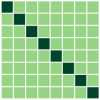
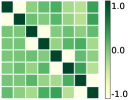
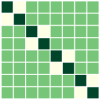
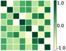
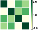
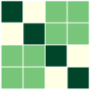
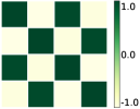
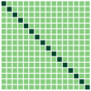
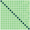
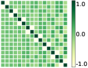
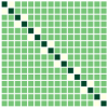
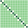
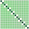
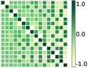
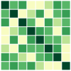
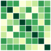
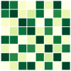
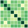
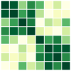
First, we compare the minimizers of three optimization problems: (i) full-batch optimization in Eq.(1); (ii) mini-batch optimization in Eq. (4) with 𝒮B=[(NB)]{\mathcal{S}}_{B}=\left[\binom{N}{B}\right]; (iii) mini-batch optimization with 𝒮B[(NB)]{\mathcal{S}}_{B}\subsetneq\left[\binom{N}{B}\right]. We apply GD algorithm to each problem for N=8N=8 and B=2B=2, obtain the updated embedding matrices, and then show the heatmap plot of N×NN\times N gram matrix containing all the pairwise inner products 𝒖i𝒗j{\bm{u}}_{i}^{\intercal}{\bm{v}}_{j} in Fig. 4(b)-(d). Here, we plot for two regimes: d=2Nd=2N for the top row, and d=N/2d=N/2 for the bottom row. In Fig. 4(a), we plot the gram matrix for the optimal solution obtained in Sec. 4.2. One can observe that when either full-batch or all (NB)\binom{N}{B} mini-batches are used for training, the trained embedding vectors reach a simplex ETF and simplex cross-polytope solutions for d=2Nd=2N and d=N/2d=N/2, respectively, as proved in Thm 4. In contrast, when a strict subset of (NB)\binom{N}{B} mini-batches are used for training, these solutions are not achieved.

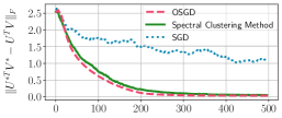
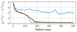
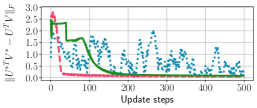
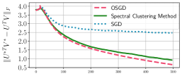
Second, we compare the convergence speed of three algorithms in mini-batch optimization: (i) OSGD; (ii) the proposed SC method; and (iii) SGD (see details of the algorithms in Appendix C). Fig. 4(e) shows the 𝑼𝑽𝑼(t)𝑽(t)F\|{\bm{U}}^{\star\intercal}{\bm{V}}^{\star}-{\bm{U}}^{(t)\intercal}{\bm{V}}^{(t)}\|_{F} which is the Frobenius norm of the difference between heatmaps of the ground-truth solution (𝑼,𝑽{\bm{U}}^{\star},{\bm{V}}^{\star}) and the embeddings at each step tt. We restrict the number of updates for all algorithms, specifically 500 steps. We observe that both OSGD and the proposed method nearly converge to the ground-truth solutions proved in Thm. 4 within 500 steps, while SGD does not. We obtain similar results for other values of NN and dd, given in Appendix D.2.

Table 1: Top-1 retrieval accuracy on CIFAR-100-C (or Tiny ImageNet-C) [23], when each algorithm uses CIFAR-100 (or Tiny ImageNet) to pretrain ResNet-18 with SimCLR and SogCLR objective. SC algorithm proposed in Sec. 5.3 outperforms all baselines.
CIFAR-100 Tiny ImageNet
SimCLR SogCLR SimCLR SogCLR
OSGD 31.4 ±\pm 0.03 23.8 ±\pm 0.02 33.6 ±\pm 0.04 29.7 ±\pm 0.04
SGD 31.3 ±\pm 0.02 23.6 ±\pm 0.05 33.2 ±\pm 0.03 28.6 ±\pm 0.03
SC 32.5\bm{32.5} ±\pm 0.05 30.0\bm{30.0} ±\pm 0.04 33.8\bm{33.8} ±\pm 0.04 33.3\bm{33.3} ±\pm 0.03

6.2 Real Datasets

Here we show that the proposed SC method is effective in more practical settings where the embedding is learned by a parameterized encoder, and can be easily applied to existing uni-modal frameworks, such as SimCLR [9] and SogCLR [68]. We conduct mini-batch contrastive learning on CIFAR-100 and Tiny ImageNet datasets and report the performances in the image retrieval downstream task on corrupted datasets, the results of which are in Table 1. Due to the page limit, we provide detailed experimental information in the Appendix D.3.

7 Conclusion

We provided a thorough theoretical analysis of mini-batch contrastive learning. First, we showed that the solution of mini-batch optimization and that of full-batch optimization are identical if and only if all (NB){N\choose B} mini-batches are considered. Second, we analyzed the convergence of OSGD and devised spectral clustering (SC) method, a new batch selection method which handles the complexity issue of OSGD in mini-batch contrastive learning. Experimental results support our theoretical findings and the efficacy of SC.

Limitations

We note that our theoretical results have two major limitations:

  1. 1.

    While we would like to extend our results to the general case of N>d+1N>d+1, we were only able to characterize the optimal solution for the specific case of N=2dN=2d. Furthermore, our result for the case of N=2dN=2d in Thm. 4 requires the use of the conjecture that the optimal solution is symmetric and antipodal. However, as mentioned by Lu & Steinerberger [36], the general case of N>d+1N>d+1 seems quite challenging in the non-asymptotic regime.

  2. 2.

    In practice, the embeddings are usually the output of a shared neural network encoder. However, our results are for the case when the embeddings only have a norm constraint. Thus, our results do not readily indicate any generalization to unseen data. We expect however, that it is possible to extend our results to the shared encoder setting by assuming sufficient overparameterization.

References

  • Aberdam et al. [2021] Aberdam, A., Litman, R., Tsiper, S., Anschel, O., Slossberg, R., Mazor, S., Manmatha, R., and Perona, P. Sequence-to-sequence contrastive learning for text recognition. In Proceedings of the IEEE/CVF Conference on Computer Vision and Pattern Recognition, pp.  15302–15312, 2021.
  • Ahn et al. [2020] Ahn, K., Yun, C., and Sra, S. Sgd with shuffling: optimal rates without component convexity and large epoch requirements. Advances in Neural Information Processing Systems, 33:17526–17535, 2020.
  • Bachman et al. [2019] Bachman, P., Hjelm, R. D., and Buchwalter, W. Learning representations by maximizing mutual information across views. Advances in neural information processing systems, 32, 2019.
  • Borodachov [2022] Borodachov, S. Optimal antipodal configuration of 2d2d points on a sphere in d\mathbb{R}^{d} for covering. arXiv preprint arXiv:2210.12472, 2022.
  • Bottou [2009] Bottou, L. Curiously fast convergence of some stochastic gradient descent algorithms. In Proceedings of the symposium on learning and data science, Paris, volume 8, pp.  2624–2633, 2009.
  • Cha et al. [2023] Cha, J., Lee, J., and Yun, C. Tighter lower bounds for shuffling sgd: Random permutations and beyond, 2023.
  • Chen et al. [2022] Chen, C., Zhang, J., Xu, Y., Chen, L., Duan, J., Chen, Y., Tran, S. D., Zeng, B., and Chilimbi, T. Why do we need large batchsizes in contrastive learning? a gradient-bias perspective. In Oh, A. H., Agarwal, A., Belgrave, D., and Cho, K. (eds.), Advances in Neural Information Processing Systems, 2022.
  • Chen et al. [2021] Chen, H., Lagadec, B., and Bremond, F. Ice: Inter-instance contrastive encoding for unsupervised person re-identification. In Proceedings of the IEEE/CVF International Conference on Computer Vision, pp.  14960–14969, 2021.
  • Chen et al. [2020a] Chen, T., Kornblith, S., Norouzi, M., and Hinton, G. A simple framework for contrastive learning of visual representations. In International conference on machine learning, pp. 1597–1607. PMLR, 2020a.
  • Chen et al. [2020b] Chen, X., Fan, H., Girshick, R., and He, K. Improved baselines with momentum contrastive learning. arXiv preprint arXiv:2003.04297, 2020b.
  • Cho & Yun [2023] Cho, H. and Yun, C. Sgda with shuffling: faster convergence for nonconvex-pł minimax optimization, 2023.
  • Chopra et al. [2005] Chopra, S., Hadsell, R., and LeCun, Y. Learning a similarity metric discriminatively, with application to face verification. In 2005 IEEE Computer Society Conference on Computer Vision and Pattern Recognition (CVPR’05), volume 1, pp.  539–546. IEEE, 2005.
  • Cormen et al. [2022] Cormen, T. H., Leiserson, C. E., Rivest, R. L., and Stein, C. Introduction to algorithms. MIT press, 2022.
  • Crouse [2016] Crouse, D. F. On implementing 2d rectangular assignment algorithms. IEEE Transactions on Aerospace and Electronic Systems, 52(4):1679–1696, 2016.
  • Davis & Drusvyatskiy [2019] Davis, D. and Drusvyatskiy, D. Stochastic model-based minimization of weakly convex functions. SIAM Journal on Optimization, 29(1):207–239, 2019.
  • Elizalde et al. [2023] Elizalde, B., Deshmukh, S., Ismail, M. A., and Wang, H. Clap learning audio concepts from natural language supervision. In ICASSP 2023 - 2023 IEEE International Conference on Acoustics, Speech and Signal Processing (ICASSP), pp.  1–5, 2023.
  • Gadre et al. [2023] Gadre, S. Y., Ilharco, G., Fang, A., Hayase, J., Smyrnis, G., Nguyen, T., Marten, R., Wortsman, M., Ghosh, D., Zhang, J., et al. Datacomp: In search of the next generation of multimodal datasets. arXiv preprint arXiv:2304.14108, 2023.
  • Goel et al. [2022] Goel, S., Bansal, H., Bhatia, S., Rossi, R., Vinay, V., and Grover, A. Cyclip: Cyclic contrastive language-image pretraining. In Advances in Neural Information Processing Systems, volume 35, pp.  6704–6719. Curran Associates, Inc., 2022.
  • Grill et al. [2020] Grill, J.-B., Strub, F., Altché, F., Tallec, C., Richemond, P., Buchatskaya, E., Doersch, C., Avila Pires, B., Guo, Z., Gheshlaghi Azar, M., et al. Bootstrap your own latent-a new approach to self-supervised learning. Advances in neural information processing systems, 33:21271–21284, 2020.
  • Gürbüzbalaban et al. [2021] Gürbüzbalaban, M., Ozdaglar, A., and Parrilo, P. A. Why random reshuffling beats stochastic gradient descent. Mathematical Programming, 186(1):49–84, 2021.
  • Haochen & Sra [2019] Haochen, J. and Sra, S. Random shuffling beats sgd after finite epochs. In International Conference on Machine Learning, pp. 2624–2633. PMLR, 2019.
  • He et al. [2020] He, K., Fan, H., Wu, Y., Xie, S., and Girshick, R. Momentum contrast for unsupervised visual representation learning. In Proceedings of the IEEE/CVF conference on computer vision and pattern recognition, pp.  9729–9738, 2020.
  • Hendrycks & Dietterich [2019] Hendrycks, D. and Dietterich, T. G. Benchmarking neural network robustness to common corruptions and perturbations. In 7th International Conference on Learning Representations, ICLR 2019, 2019.
  • Hu et al. [2021] Hu, Q., Wang, X., Hu, W., and Qi, G.-J. Adco: Adversarial contrast for efficient learning of unsupervised representations from self-trained negative adversaries. In Proceedings of the IEEE/CVF Conference on Computer Vision and Pattern Recognition, pp.  1074–1083, 2021.
  • Jaiswal et al. [2020] Jaiswal, A., Babu, A. R., Zadeh, M. Z., Banerjee, D., and Makedon, F. A survey on contrastive self-supervised learning. Technologies, 9(1):2, 2020.
  • Ji et al. [2022] Ji, W., Lu, Y., Zhang, Y., Deng, Z., and Su, W. J. An unconstrained layer-peeled perspective on neural collapse. In International Conference on Learning Representations, 2022.
  • Jia et al. [2021] Jia, C., Yang, Y., Xia, Y., Chen, Y.-T., Parekh, Z., Pham, H., Le, Q., Sung, Y.-H., Li, Z., and Duerig, T. Scaling up visual and vision-language representation learning with noisy text supervision. In International Conference on Machine Learning, pp. 4904–4916. PMLR, 2021.
  • Kalantidis et al. [2020] Kalantidis, Y., Sariyildiz, M. B., Pion, N., Weinzaepfel, P., and Larlus, D. Hard negative mixing for contrastive learning. Advances in Neural Information Processing Systems, 33:21798–21809, 2020.
  • Kawaguchi & Lu [2020] Kawaguchi, K. and Lu, H. Ordered sgd: A new stochastic optimization framework for empirical risk minimization. In International Conference on Artificial Intelligence and Statistics, pp.  669–679. PMLR, 2020.
  • Khosla et al. [2020] Khosla, P., Teterwak, P., Wang, C., Sarna, A., Tian, Y., Isola, P., Maschinot, A., Liu, C., and Krishnan, D. Supervised contrastive learning. Advances in Neural Information Processing Systems, 33:18661–18673, 2020.
  • Krizhevsky et al. [2009] Krizhevsky, A., Hinton, G., et al. Learning multiple layers of features from tiny images. 2009.
  • Kuhn [1955] Kuhn, H. W. The hungarian method for the assignment problem. Naval research logistics quarterly, 2(1-2):83–97, 1955.
  • Le & Yang [2015] Le, Y. and Yang, X. Tiny imagenet visual recognition challenge. CS 231N, 7(7):3, 2015.
  • Lee et al. [2022] Lee, J., Kim, J., Shon, H., Kim, B., Kim, S. H., Lee, H., and Kim, J. UniCLIP: Unified framework for contrastive language-image pre-training. In Advances in Neural Information Processing Systems, 2022.
  • Loshchilov & Hutter [2015] Loshchilov, I. and Hutter, F. Online batch selection for faster training of neural networks. arXiv preprint arXiv:1511.06343, 2015.
  • Lu & Steinerberger [2022] Lu, J. and Steinerberger, S. Neural collapse under cross-entropy loss. Applied and Computational Harmonic Analysis, 59:224–241, 2022. ISSN 1063-5203. Special Issue on Harmonic Analysis and Machine Learning.
  • Lu et al. [2021] Lu, Y., Meng, S. Y., and De Sa, C. A general analysis of example-selection for stochastic gradient descent. In International Conference on Learning Representations, 2021.
  • Lu et al. [2022] Lu, Y., Guo, W., and Sa, C. D. Grab: Finding provably better data permutations than random reshuffling. In Advances in Neural Information Processing Systems, 2022.
  • Ma et al. [2021] Ma, S., Zeng, Z., McDuff, D., and Song, Y. Active contrastive learning of audio-visual video representations. In International Conference on Learning Representations, 2021.
  • Mishchenko et al. [2020] Mishchenko, K., Khaled, A., and Richtárik, P. Random reshuffling: Simple analysis with vast improvements. Advances in Neural Information Processing Systems, 33:17309–17320, 2020.
  • Misra & Maaten [2020] Misra, I. and Maaten, L. v. d. Self-supervised learning of pretext-invariant representations. In Proceedings of the IEEE/CVF Conference on Computer Vision and Pattern Recognition, pp.  6707–6717, 2020.
  • Nagaraj et al. [2019] Nagaraj, D., Jain, P., and Netrapalli, P. Sgd without replacement: Sharper rates for general smooth convex functions. In International Conference on Machine Learning, pp. 4703–4711. PMLR, 2019.
  • Ng et al. [2001] Ng, A., Jordan, M., and Weiss, Y. On spectral clustering: Analysis and an algorithm. Advances in neural information processing systems, 14, 2001.
  • Nguyen et al. [2021] Nguyen, L. M., Tran-Dinh, Q., Phan, D. T., Nguyen, P. H., and Van Dijk, M. A unified convergence analysis for shuffling-type gradient methods. The Journal of Machine Learning Research, 22(1):9397–9440, 2021.
  • Oord et al. [2018] Oord, A. v. d., Li, Y., and Vinyals, O. Representation learning with contrastive predictive coding. arXiv preprint arXiv:1807.03748, 2018.
  • Papyan et al. [2020] Papyan, V., Han, X., and Donoho, D. L. Prevalence of neural collapse during the terminal phase of deep learning training. Proceedings of the National Academy of Sciences, 117(40):24652–24663, 2020.
  • Pham et al. [2021] Pham, H., Dai, Z., Ghiasi, G., Liu, H., Yu, A. W., Luong, M.-T., Tan, M., and Le, Q. V. Combined scaling for zero-shot transfer learning. arXiv preprint arXiv:2111.10050, 2021.
  • Radford et al. [2021] Radford, A., Kim, J. W., Hallacy, C., Ramesh, A., Goh, G., Agarwal, S., Sastry, G., Askell, A., Mishkin, P., Clark, J., et al. Learning transferable visual models from natural language supervision. In International Conference on Machine Learning, pp. 8748–8763. PMLR, 2021.
  • Rajput et al. [2020] Rajput, S., Gupta, A., and Papailiopoulos, D. Closing the convergence gap of sgd without replacement. In International Conference on Machine Learning, pp. 7964–7973. PMLR, 2020.
  • Rajput et al. [2022] Rajput, S., Lee, K., and Papailiopoulos, D. Permutation-based SGD: Is random optimal? In International Conference on Learning Representations, 2022.
  • Ramesh et al. [2021] Ramesh, A., Pavlov, M., Goh, G., Gray, S., Voss, C., Radford, A., Chen, M., and Sutskever, I. Zero-shot text-to-image generation. In International Conference on Machine Learning, pp. 8821–8831. PMLR, 2021.
  • Ramesh et al. [2022] Ramesh, A., Dhariwal, P., Nichol, A., Chu, C., and Chen, M. Hierarchical text-conditional image generation with clip latents. arXiv preprint arXiv:2204.06125, 2022.
  • Recht & Re [2012] Recht, B. and Re, C. Toward a noncommutative arithmetic-geometric mean inequality: Conjectures, case-studies, and consequences. In Proceedings of the 25th Annual Conference on Learning Theory, volume 23 of Proceedings of Machine Learning Research, pp. 11.1–11.24. PMLR, 2012.
  • Recht & Ré [2013] Recht, B. and Ré, C. Parallel stochastic gradient algorithms for large-scale matrix completion. Mathematical Programming Computation, 5(2):201–226, 2013.
  • Robinson et al. [2021] Robinson, J. D., Chuang, C.-Y., Sra, S., and Jegelka, S. Contrastive learning with hard negative samples. In International Conference on Learning Representations, 2021.
  • Sachidananda et al. [2022] Sachidananda, V., Tseng, S.-Y., Marchi, E., Kajarekar, S., and Georgiou, P. Calm: Contrastive aligned audio-language multirate and multimodal representations. arXiv preprint arXiv:2202.03587, 2022.
  • Safran & Shamir [2021a] Safran, I. and Shamir, O. How good is sgd with random shuffling?, 2021a.
  • Safran & Shamir [2021b] Safran, I. and Shamir, O. Random shuffling beats sgd only after many epochs on ill-conditioned problems. Advances in Neural Information Processing Systems, 34:15151–15161, 2021b.
  • Schroff et al. [2015] Schroff, F., Kalenichenko, D., and Philbin, J. Facenet: A unified embedding for face recognition and clustering. In Proceedings of the IEEE conference on computer vision and pattern recognition, pp.  815–823, 2015.
  • Sohn [2016] Sohn, K. Improved deep metric learning with multi-class n-pair loss objective. Advances in neural information processing systems, 29, 2016.
  • Song & Ermon [2020] Song, J. and Ermon, S. Understanding the limitations of variational mutual information estimators. In International Conference on Learning Representations, 2020.
  • Sustik et al. [2007] Sustik, M. A., Tropp, J. A., Dhillon, I. S., and Heath Jr, R. W. On the existence of equiangular tight frames. Linear Algebra and its applications, 426(2-3):619–635, 2007.
  • Tran et al. [2021] Tran, T. H., Nguyen, L. M., and Tran-Dinh, Q. Smg: A shuffling gradient-based method with momentum. In Meila, M. and Zhang, T. (eds.), Proceedings of the 38th International Conference on Machine Learning, volume 139 of Proceedings of Machine Learning Research, pp.  10379–10389. PMLR, 2021.
  • Wang & Qi [2022] Wang, X. and Qi, G.-J. Contrastive learning with stronger augmentations. IEEE Transactions on Pattern Analysis and Machine Intelligence, 2022.
  • Yeh et al. [2022] Yeh, C.-H., Hong, C.-Y., Hsu, Y.-C., Liu, T.-L., Chen, Y., and LeCun, Y. Decoupled contrastive learning. In European Conference on Computer Vision, pp.  668–684. Springer, 2022.
  • Ying et al. [2020] Ying, B., Yuan, K., and Sayed, A. H. Variance-reduced stochastic learning under random reshuffling. IEEE Transactions on Signal Processing, 68:1390–1408, 2020. doi: 10.1109/TSP.2020.2968280.
  • You et al. [2017] You, Y., Gitman, I., and Ginsburg, B. Large batch training of convolutional networks. arXiv preprint arXiv:1708.03888, 2017.
  • Yuan et al. [2022] Yuan, Z., Wu, Y., Qiu, Z.-H., Du, X., Zhang, L., Zhou, D., and Yang, T. Provable stochastic optimization for global contrastive learning: Small batch does not harm performance. In International Conference on Machine Learning, pp. 25760–25782. PMLR, 2022.
  • Zeng et al. [2021] Zeng, D., Wu, Y., Hu, X., Xu, X., Yuan, H., Huang, M., Zhuang, J., Hu, J., and Shi, Y. Positional contrastive learning for volumetric medical image segmentation. In Medical Image Computing and Computer Assisted Intervention–MICCAI 2021: 24th International Conference, Strasbourg, France, September 27–October 1, 2021, Proceedings, Part II 24, pp.  221–230. Springer, 2021.
  • Zhang & Stratos [2021] Zhang, W. and Stratos, K. Understanding hard negatives in noise contrastive estimation. In North American Chapter of the Association for Computational Linguistics, 2021.
  • Zhou et al. [2022] Zhou, J., Li, X., Ding, T., You, C., Qu, Q., and Zhu, Z. On the optimization landscape of neural collapse under mse loss: Global optimality with unconstrained features. In International Conference on Machine Learning, pp. 27179–27202. PMLR, 2022.
  • Zolfaghari et al. [2021] Zolfaghari, M., Zhu, Y., Gehler, P., and Brox, T. Crossclr: Cross-modal contrastive learning for multi-modal video representations. In Proceedings of the IEEE/CVF International Conference on Computer Vision, pp.  1450–1459, 2021.

Organization of the Appendix

  1. 1.

    In Appendix A, we introduce an additional definition for posterity.

  2. 2.

    In Appendix B, we provide detailed proofs of the theoretical results as well as any intermediate results/lemmas that we found useful.

    1. (a)

      Appendix B.1 provides proofs of the results from Section 4 which focuses on the relationship between the optimal solutions for minimizing the mini-batch and full-batch constrastive loss.

    2. (b)

      Appendix B.2 contains the proofs of results from Section 5 which concern the application of Ordered SGD to mini-batch contrastive learning.

    3. (c)

      Appendix B.3 is intended to supplement Appendix B.2. It contains auxiliary notation and proofs required in the proof of Theorem 7.

  3. 3.

    Appendix C specifies the pseudo-code and details for the three algorithms: (i) Spectral Clustering; (ii) Stochastic Gradient Descent (SGD) and (iii) Ordered SGD (OSGD).

  4. 4.

    Appendix D describes the details of the experimental settings from Section 6 while also providing some additional results.

Appendix A Additional Definition

Definition 4 (Sustik et al. [62]).

A set of NN vectors {𝒖i}i=1N\{{\bm{u}}_{i}\}_{i=1}^{N} in the d\mathbb{R}^{d} form an equiangular tight frame (ETF) if (i) they are all unit norm: 𝒖i=1\lVert{\bm{u}}_{i}\rVert=1 for every i[N]i\in[N], (ii) they are equiangular: 𝒖i𝒖j=α0\lVert{\bm{u}}_{i}^{\intercal}{\bm{u}}_{j}\rVert=\alpha\geq 0 for all iji\neq j and some α0\alpha\geq 0, and (iii) they form a tight frame: 𝑼𝑼=(N/d)𝕀d{\bm{U}}{\bm{U}}^{\intercal}=(N/d)\mathbb{I}_{d} where 𝑼{\bm{U}} is a d×Nd\times N matrix whose columns are 𝒖1,𝒖2,,𝒖N{\bm{u}}_{1},{\bm{u}}_{2},\dots,{\bm{u}}_{N}, and 𝕀d\mathbb{I}_{d} is the d×dd\times d identity matrix.

Appendix B Proofs

B.1 Proofs of Results From Section 4

See 1

Proof.

First, we define the contrastive loss as the sum of two symmetric one-sided contrastive loss terms to simplify the notation. We denote the following term as the one-sided contrastive loss

(𝑼,𝑽)=1Ni=1Nlog(e𝒖i𝒗ij=1Ne𝒖i𝒗j).{\mathcal{L}}({\bm{U}},{\bm{V}})=\frac{1}{N}\sum_{i=1}^{N}-\log\left(\frac{e^{{\bm{u}}_{i}^{\intercal}{\bm{v}}_{i}}}{\sum_{j=1}^{N}e^{{\bm{u}}_{i}^{\intercal}{\bm{v}}_{j}}}\right). (6)

Then, the overall contrastive loss is given by the sum of the two one-sided contrastive losses:

con(𝑼,𝑽)=(𝑼,𝑽)+(𝑽,𝑼).{\mathcal{L}}^{\operatorname{con}}({\bm{U}},{\bm{V}})={\mathcal{L}}({\bm{U}},{\bm{V}})+{\mathcal{L}}({\bm{V}},{\bm{U}}). (7)

Since con{\mathcal{L}}^{\operatorname{con}} is symmetric in its arguments, results pertaining to the optimum of (𝑼,𝑽){\mathcal{L}}({\bm{U}},{\bm{V}}) readily extend to con{\mathcal{L}}^{\operatorname{con}}. Now, let us consider the simpler problem of minimizing the one-sided contrastive loss from Eq. (6) which reduces the problem to exactly the same setting as Lu & Steinerberger [36]:

(𝑼,𝑽)\displaystyle{\mathcal{L}}({\bm{U}},{\bm{V}}) =1Ni=1Nlog(e𝒖i𝒗ij=1Ne𝒖i𝒗j)\displaystyle=\frac{1}{N}\sum_{i=1}^{N}-\log\left(\frac{e^{{\bm{u}}_{i}^{\intercal}{\bm{v}}_{i}}}{\sum_{j=1}^{N}e^{{\bm{u}}_{i}^{\intercal}{\bm{v}}_{j}}}\right)
=1Ni=1Nlog(1+j=1,jiNe(𝒗j𝒗i)𝒖i).\displaystyle=\frac{1}{N}\sum_{i=1}^{N}\log\left(1+\sum_{{j=1,j\neq i}}^{N}e^{({\bm{v}}_{j}-{\bm{v}}_{i})^{\intercal}{\bm{u}}_{i}}\right).

Note that, we have for any fixed 1iN,1\leq i\leq N,

j=1,jiNe(𝒗j𝒗i)𝒖i\displaystyle\sum_{{j=1,j\neq i}}^{N}e^{({\bm{v}}_{j}-{\bm{v}}_{i})^{\intercal}{\bm{u}}_{i}} =e(𝒗i𝒖i)j=1,jiNe𝒗j𝒖i\displaystyle=e^{-({\bm{v}}_{i}^{\intercal}{\bm{u}}_{i})}\sum_{{j=1,j\neq i}}^{N}e^{{\bm{v}}_{j}^{\intercal}{\bm{u}}_{i}}
=(N1)e(𝒗i𝒖i)(1N1)j=1,jiNe𝒗j𝒖i\displaystyle=(N-1)e^{-({\bm{v}}_{i}^{\intercal}{\bm{u}}_{i})}\left(\frac{1}{N-1}\right)\sum_{{j=1,j\neq i}}^{N}e^{{\bm{v}}_{j}^{\intercal}{\bm{u}}_{i}}
(a)(N1)e(𝒗i𝒖i)exp(1N1j=1,jiN𝒗j𝒖i)\displaystyle\overset{(a)}{\geq}(N-1)e^{-({\bm{v}}_{i}^{\intercal}{\bm{u}}_{i})}\exp\left(\frac{1}{N-1}\sum_{{j=1,j\neq i}}^{N}{\bm{v}}_{j}^{\intercal}{\bm{u}}_{i}\right)
=(b)(N1)e(𝒗i𝒖i)exp(𝒗𝒖i𝒗i𝒖iN1)\displaystyle\overset{(b)}{=}(N-1)e^{-({\bm{v}}_{i}^{\intercal}{\bm{u}}_{i})}\exp\left(\frac{{\bm{v}}^{\intercal}{\bm{u}}_{i}-{\bm{v}}_{i}^{\intercal}{\bm{u}}_{i}}{N-1}\right)
=(N1)exp(𝒗𝒖iN(𝒗i𝒖i)N1),\displaystyle=(N-1)\exp\left(\frac{{\bm{v}}^{\intercal}{\bm{u}}_{i}-N({\bm{v}}_{i}^{\intercal}{\bm{u}}_{i})}{N-1}\right), (8)

where (a)(a) follows by applying Jensen inequality for ete^{t} and (b)(b) follows from 𝒗:=i=1N𝒗i{\bm{v}}:=\sum_{i=1}^{N}{\bm{v}}_{i}. Since log()\log(\cdot) is monotonic, we have that x>ylog(x)>log(y)x>y\Rightarrow\log(x)>\log(y) and therefore,

(𝑼,𝑽)\displaystyle{\mathcal{L}}({\bm{U}},{\bm{V}}) 1Ni=1Nlog[1+(N1)exp(𝒗𝒖iN1N(𝒗i𝒖i)N1)]\displaystyle\geq{1\over N}\sum_{i=1}^{N}\log\left[1+(N-1)\exp\left(\frac{{\bm{v}}^{\intercal}{\bm{u}}_{i}}{N-1}-\frac{N({\bm{v}}_{i}^{\intercal}{\bm{u}}_{i})}{N-1}\right)\right]
(c)log[1+(N1)exp(1Ni=1N(𝒗𝒖iN1N(𝒗i𝒖i)N1))]\displaystyle\overset{(c)}{\geq}\log\left[1+(N-1)\exp\left(\frac{1}{N}\sum_{i=1}^{N}\left(\frac{{\bm{v}}^{\intercal}{\bm{u}}_{i}}{N-1}-\frac{N({\bm{v}}_{i}^{\intercal}{\bm{u}}_{i})}{N-1}\right)\right)\right]
=(d)log[1+(N1)exp(1N(𝒗𝒖N1NN1i=1N(𝒗i𝒖i)))],\displaystyle\overset{(d)}{=}\log\left[1+(N-1)\exp\left(\frac{1}{N}\left(\frac{{\bm{v}}^{\intercal}{\bm{u}}}{N-1}-\frac{N}{N-1}\sum_{i=1}^{N}({\bm{v}}_{i}^{\intercal}{\bm{u}}_{i})\right)\right)\right], (9)

where (c)(c) follows by applying Jensen inequality to the convex function ϕ(t)=log(1+aebt)\phi(t)=\log(1+ae^{bt}) for a,b>0a,b>0, and (d)(d) follow from 𝒖:=i=1N𝒖i{\bm{u}}:=\sum_{i=1}^{N}{\bm{u}}_{i}.

Note that for equalities to hold in Eq. (8) and (9), we need constants ci,cc_{i},c such that

𝒗j𝒖i=ciji,\displaystyle{\bm{v}}_{j}^{\intercal}{\bm{u}}_{i}=c_{i}\quad\forall j\neq i, (10)
𝒗𝒖iN1N(𝒗i𝒖i)N1=ci[N].\displaystyle\frac{{\bm{v}}^{\intercal}{\bm{u}}_{i}}{N-1}-\frac{N({\bm{v}}_{i}^{\intercal}{\bm{u}}_{i})}{N-1}=c\quad\forall i\in[N]. (11)

Since log()\log(\cdot) and exp()\exp(\cdot) are both monotonic, minimizing the lower bound in Eq. (8) is equivalent to

min\displaystyle\min\quad 𝒗𝒖N1NN1i=1N𝒗i𝒖i\displaystyle\frac{{\bm{v}}^{\intercal}{\bm{u}}}{N-1}-\frac{N}{N-1}\sum_{i=1}^{N}{\bm{v}}_{i}^{\intercal}{\bm{u}}_{i}
max\displaystyle\Leftrightarrow\max\quad Ni=1N𝒗i𝒖i(i=1N𝒗i)(i=1N𝒖i).\displaystyle N\sum_{i=1}^{N}{\bm{v}}_{i}^{\intercal}{\bm{u}}_{i}-\Big{(}\sum_{i=1}^{N}{\bm{v}}_{i}\Big{)}^{\intercal}\Big{(}\sum_{i=1}^{N}{\bm{u}}_{i}\Big{)}. (12)

All that remains is to show that the solution that maximizes Eq 12 also satisfies the conditions in Eq. (10) and (11). To see this, first note that the maximization problem can be written as

max𝒗stack((N𝕀N𝟏N𝟏N)𝕀d)𝒖stack\displaystyle\max\quad{\bm{v}}_{\text{stack}}^{\intercal}((N\mathbb{I}_{N}-\mathbf{1}_{N}\mathbf{1}_{N}^{\intercal})\otimes\mathbb{I}_{d}){\bm{u}}_{\text{stack}}

where 𝒗stack=(𝒗1,𝒗2,,𝒗n){\bm{v}}_{\text{stack}}=({\bm{v}}_{1},{\bm{v}}_{2},\dots,{\bm{v}}_{n}) is a vector in Nd\mathbb{R}^{Nd} formed by stacking the vectors 𝒗i{\bm{v}}_{i} together. 𝒖stack{\bm{u}}_{\text{stack}} is similarly defined. 𝕀N\mathbb{I}_{N} denotes the N×NN\times N identity matrix, 𝟏N\mathbf{1}_{N} denotes the all-one vector in n\mathbb{R}^{n}, and \otimes denotes the Kronecker product. It is easy to see that 𝒖stack=𝒗stack=N\lVert{\bm{u}}_{\text{stack}}\rVert=\lVert{\bm{v}}_{\text{stack}}\rVert=\sqrt{N} since each 𝒖i=𝒗i=1\lVert{\bm{u}}_{i}\rVert=\lVert{\bm{v}}_{i}\rVert=1. Since the eigenvalues of ABA\otimes B are the product of the eigenvalues of AA and BB, in order to analyze the spectrum of the middle term in the above maximization problem, it suffices to just consider the eigenvalues of (N𝕀N𝟏N𝟏N)(N\mathbb{I}_{N}-\mathbf{1}_{N}\mathbf{1}_{N}^{\intercal}). As shown by the elegant analysis in Lu & Steinerberger [36], (N𝕀N𝟏N𝟏N)𝒑=N𝒑(N\mathbb{I}_{N}-\mathbf{1}_{N}\mathbf{1}_{N}^{\intercal}){\bm{p}}=N{\bm{p}} for any 𝒑N{\bm{p}}\in\mathbb{R}^{N} such that i=1N𝒑i=0\sum_{i=1}^{N}{\bm{p}}_{i}=0 and (N𝕀N𝟏N𝟏N)𝒒=0(N\mathbb{I}_{N}-\mathbf{1}_{N}\mathbf{1}_{N}^{\intercal}){\bm{q}}=0 for any 𝒒N{\bm{q}}\in\mathbb{R}^{N} such that 𝒒=k𝟏N{\bm{q}}=k\mathbf{1}_{N} for some kk\in\mathbb{R}. Therefore it follows that its eigenvalues are NN with multiplicity (N1)(N-1) and 0. Since its largest eigenvalue is NN and since 𝒖stack=𝒗stack=N\lVert{\bm{u}}_{\text{stack}}\rVert=\lVert{\bm{v}}_{\text{stack}}\rVert=\sqrt{N}, applying cauchy schwarz inequality, we have that

max𝒗stack(N𝕀N𝟏N𝟏N)𝕀d)𝒖stack\displaystyle\max\quad{\bm{v}}_{\text{stack}}^{\intercal}(N\mathbb{I}_{N}-\mathbf{1}_{N}\mathbf{1}_{N}^{\intercal})\otimes\mathbb{I}_{d}){\bm{u}}_{\text{stack}}^{\intercal}
=𝒗stack(N𝕀n𝟏n𝟏n)𝕀d)𝒖stack\displaystyle=\lVert{\bm{v}}_{\text{stack}}\rVert\cdot\lVert(N\mathbb{I}_{n}-\mathbf{1}_{n}\mathbf{1}_{n}^{\intercal})\otimes\mathbb{I}_{d})\rVert\cdot\lVert{\bm{u}}_{\text{stack}}\rVert
=N(N)N\displaystyle=\sqrt{N}(N)\sqrt{N}
=N2.\displaystyle=N^{2}.

Moreover, we see that setting 𝒖i=𝒗i{\bm{u}}_{i}={\bm{v}}_{i} and setting {𝒖i}i=1N\{{\bm{u}}_{i}\}_{i=1}^{N} to be the simplex ETF attains the maximum above while also satisfying the conditions in Eq. (10) and (11) with ci=1/(N1)c_{i}=-1/(N-1) and c=N/(N1)c=-N/(N-1). Therefore, the inequalities in Eq. (8) and (9) are actually equalities for 𝒖i=𝒗i{\bm{u}}_{i}={\bm{v}}_{i} when they are chosen to be the simplex ETF in d\mathbb{R}^{d} which is attainable since dN1d\geq N-1. Therefore, we have shown that if 𝑼={𝒖i}i=1N{\bm{U}}^{\star}=\{{\bm{u}}_{i}^{\star}\}_{i}=1^{N} is the simplex ETF and 𝒖i=𝒗ii[N]{\bm{u}}_{i}^{\star}={\bm{v}}_{i}^{\star}\;\forall i\in[N], then 𝑼,𝑽=argmin𝑼,𝑽(𝑼,𝑽){\bm{U}}^{\star},{\bm{V}}^{\star}=arg\min_{{\bm{U}},{\bm{V}}}{\mathcal{L}}({\bm{U}},{\bm{V}}) over the unit sphere in n\mathbb{R}^{n}. All that remains is to show that this is also the minimizer for con{\mathcal{L}}^{\operatorname{con}}.

First note that 𝑼,𝑽{\bm{U}}^{\star},{\bm{V}}^{\star} is also the minimizer for (𝑽,𝑼){\mathcal{L}}({\bm{V}},{\bm{U}}) through symmetry. One can repeat the proof exactly by simply exchanging 𝒖i{\bm{u}}_{i} and 𝒗i{\bm{v}}_{i} to see that this is indeed true. Now recalling Eq. (7), we have

mincon\displaystyle\min{\mathcal{L}}^{\operatorname{con}} =min((𝑼,𝑽)+(𝑼,𝑽))\displaystyle=\min{({\mathcal{L}}({\bm{U}},{\bm{V}})+{\mathcal{L}}({\bm{U}},{\bm{V}}))}
min((𝑼,𝑽))+min((𝑼,𝑽))\displaystyle\geq\min{({\mathcal{L}}({\bm{U}},{\bm{V}}))}+\min{({\mathcal{L}}({\bm{U}},{\bm{V}}))} (13)
=(𝑼,𝑽)+(𝑽,𝑼).\displaystyle={\mathcal{L}}({\bm{U}}^{\star},{\bm{V}}^{\star})+{\mathcal{L}}({\bm{V}}^{\star},{\bm{U}}^{\star}).

However, since the minimizer of both terms in Eq. (13) is the same, the inequality becomes an equality. Therefore, we have shown that (𝑼,𝑽){\bm{U}}^{\star},{\bm{V}}^{\star}) is the minimizer of con{\mathcal{L}}^{\operatorname{con}} completing the proof. ∎

Remark 1.

In the proof of the above Lemma, we only show that the simplex ETF attains the minimum loss in Eq. (1), but not that it is the only minimizer. The proof of Lu & Steinerberger [36] can be extended to show that this is indeed true as well. We omit it here for ease of exposition.

See 3

Proof.

By applying the logarithmic property that allows division to be represented as subtraction,

(𝑼,𝑽)\displaystyle{\mathcal{L}}({\bm{U}},{\bm{V}}) =1Ni=1Nlog(e𝒖i𝒗ij=1Ne𝒖i𝒗j)\displaystyle=-{1\over N}\sum_{i=1}^{N}\log\left(\frac{e^{{\bm{u}}_{i}^{\intercal}{\bm{v}}_{i}}}{\sum_{j=1}^{N}e^{{\bm{u}}_{i}^{\intercal}{\bm{v}}_{j}}}\right)
=1Ni=1N[𝒖i𝒗ilog(j=1Ne𝒖i𝒗j)].\displaystyle=-{1\over N}\sum_{i=1}^{N}\left[{\bm{u}}_{i}^{\intercal}{\bm{v}}_{i}-\log\Big{(}\sum_{j=1}^{N}e^{{\bm{u}}_{i}^{\intercal}{\bm{v}}_{j}}\Big{)}\right].

Since 𝑼=𝑽{\bm{U}}={\bm{V}} (symmetric property), the contrastive loss satisfies

con(𝑼,𝑽)\displaystyle{\mathcal{L}}^{\operatorname{con}}({\bm{U}},{\bm{V}}) =2(𝑼,𝑼)\displaystyle=2{\mathcal{L}}({\bm{U}},{\bm{U}})
=2Ni=1N[𝒖i𝒖ilog(j=1Ne𝒖i𝒖j)]\displaystyle=-{2\over N}\sum_{i=1}^{N}\left[{\bm{u}}_{i}^{\intercal}{\bm{u}}_{i}-\log\Big{(}\sum_{j=1}^{N}e^{{\bm{u}}_{i}^{\intercal}{\bm{u}}_{j}}\Big{)}\right]
=2+2Ni=1Nlog(j=1Ne𝒖i𝒖j).\displaystyle=-2+{2\over N}\sum_{i=1}^{N}\log\big{(}\sum_{j=1}^{N}e^{{\bm{u}}_{i}^{\intercal}{\bm{u}}_{j}}\big{)}. (14)

Since 𝒖i=1\lVert{\bm{u}}_{i}\rVert=1 for any i[N]i\in[N], we can derive the following relations:

𝒖i𝒖j2=22𝒖i𝒖j,𝒖i𝒖j=1𝒖i𝒖j22.\displaystyle\lVert{\bm{u}}_{i}-{\bm{u}}_{j}\rVert^{2}=2-2{\bm{u}}_{i}^{\intercal}{\bm{u}}_{j},\quad{\bm{u}}_{i}^{\intercal}{\bm{u}}_{j}=1-{\lVert{\bm{u}}_{i}-{\bm{u}}_{j}\rVert^{2}\over 2}.

We incorporate these relations into Eq. (23) as follows:

con(𝑼,𝑽)\displaystyle{\mathcal{L}}^{\operatorname{con}}({\bm{U}},{\bm{V}}) =2+2Ni=1Nlog(j=1Ne1𝒖i𝒖j2/2)\displaystyle=-2+{2\over N}\sum_{i=1}^{N}\log\big{(}\sum_{j=1}^{N}e^{1-\lVert{\bm{u}}_{i}-{\bm{u}}_{j}\rVert^{2}/2}\big{)}
=2Ni=1Nlog(j=1Ne𝒖i𝒖j2/2).\displaystyle={2\over N}\sum_{i=1}^{N}\log\big{(}\sum_{j=1}^{N}e^{-\lVert{\bm{u}}_{i}-{\bm{u}}_{j}\rVert^{2}/2}\big{)}.

The antipodal property of 𝑼{\bm{U}} indicates that for each i[N]i\in[N], there exists a j(i)j(i) such that uj(i)=uiu_{j(i)}=-u_{i}. By applying this property, we can manipulate the summation of e𝒖i𝒖j2/2e^{-\lVert{\bm{u}}_{i}-{\bm{u}}_{j}\rVert^{2}/2} over jj as the following:

j=1Ne𝒖i𝒖j2/2\displaystyle\sum_{j=1}^{N}e^{-\lVert{\bm{u}}_{i}-{\bm{u}}_{j}\rVert^{2}/2} =e𝒖i𝒖i2/2+e𝒖i𝒖j(i)2/2+ji,j(i)e𝒖i𝒖j2/2\displaystyle=e^{-\lVert{\bm{u}}_{i}-{\bm{u}}_{i}\rVert^{2}/2}+e^{-\lVert{\bm{u}}_{i}-{\bm{u}}_{j(i)}\rVert^{2}/2}+\sum_{j\neq i,j(i)}e^{-\lVert{\bm{u}}_{i}-{\bm{u}}_{j}\rVert^{2}/2}
=1+e2+ji,j(i)e𝒖i𝒖j2/2.\displaystyle=1+e^{-2}+\sum_{j\neq i,j(i)}e^{-\lVert{\bm{u}}_{i}-{\bm{u}}_{j}\rVert^{2}/2}.

Therefore,

con(𝑼,𝑽)=2Ni=1Nlog(1+e2+ji,j(i)e𝒖i𝒖j2/2)\displaystyle{\mathcal{L}}^{\operatorname{con}}({\bm{U}},{\bm{V}})={2\over N}\sum_{i=1}^{N}\log\Big{(}1+e^{-2}+\sum_{j\neq i,j(i)}e^{-\lVert{\bm{u}}_{i}-{\bm{u}}_{j}\rVert^{2}/2}\Big{)}
(a)2N(N2)i=1Nji,j(i)log(1+e2+(N2)e𝒖i𝒖j2/2)\displaystyle\overset{(a)}{\geq}{2\over N(N-2)}\sum_{i=1}^{N}\sum_{j\neq i,j(i)}\log\big{(}1+e^{-2}+(N-2)e^{-\lVert{\bm{u}}_{i}-{\bm{u}}_{j}\rVert^{2}/2}\big{)}
=2N(N2)i=1Njilog(1+e2+(N2)e𝒖i𝒖j2/2)2N2log(1+(N1)e2)\displaystyle={2\over N(N-2)}\sum_{i=1}^{N}\sum_{j\neq i}\log\big{(}1+e^{-2}+(N-2)e^{-\lVert{\bm{u}}_{i}-{\bm{u}}_{j}\rVert^{2}/2}\big{)}-{2\over N-2}\log(1+(N-1)e^{-2})
(b)2N(N2)i=1Njilog(1+e2+(N2)e𝒖i𝒖j2/2)2N2log(1+(N1)e2),\displaystyle\overset{(b)}{\geq}{2\over N(N-2)}\sum_{i=1}^{N}\sum_{j\neq i}\log\big{(}1+e^{-2}+(N-2)e^{-\lVert{\bm{u}}_{i}^{\star}-{\bm{u}}_{j}^{\star}\rVert^{2}/2}\big{)}-{2\over N-2}\log(1+(N-1)e^{-2}),

where (a) follows by applying Jensen’s inequality to the concave function f(t)=log(1+e2+t)f(t)=\log(1+e^{-2}+t); and (b) follows by Lem. 3, and the fact that function g(t)=log[1+e2+(N2)et/2]g(t)=\log[1+e^{-2}+(N-2)e^{-t/2}] is convex and monotonically decreasing. {𝒖1,,𝒖N}\{{\bm{u}}^{\star}_{1},\cdots,{\bm{u}}^{\star}_{N}\} denotes a set of vectors which forms a cross-polytope.

Both inequalities in (a)(a) and (b)(b) are equalities only when the columns of 𝑼{\bm{U}} form a cross-polytope. Therefore, the columns of 𝑼{\bm{U}}^{\star} form a cross-polytope. ∎

Lemma 3.

Given a function g(t)g(t) is convex and monotonically decreasing, let

𝑼:=argmin𝑼𝒜i=1Njig(𝒖i𝒖j2)s.t.𝒖i=1,𝒗i=1i[N],\displaystyle{\bm{U}}^{*}:=\arg\min\limits_{{\bm{U}}\in{\mathcal{A}}}\sum_{i=1}^{N}\sum_{j\neq i}g(\|{\bm{u}}_{i}-{\bm{u}}_{j}\|^{2})\quad\text{s.t.}\quad\|{\bm{u}}_{i}\|=1,\|{\bm{v}}_{i}\|=1\quad\forall i\in[N], (15)

where 𝒜:={𝐔:𝐔 is antipodal}{\mathcal{A}}:=\{{\bm{U}}:{\bm{U}}\text{ is antipodal}\}. Then, the columns of 𝐔{\bm{U}}^{*} form a simplex cross-polytope for N=2dN=2d.

Proof.

Suppose N=2dN=2d and 𝑼𝒜{\bm{U}}\in{\mathcal{A}}. Given a function g(t)g(t) is convex and monotonically decreasing. j(i)j(i) denotes the corresponding index for ii such that 𝒖j(i)=𝒖i{\bm{u}}_{j(i)}=-{\bm{u}}_{i}, and 𝒖i𝒖j(i)2=4\|{\bm{u}}_{i}-{\bm{u}}_{j(i)}\|^{2}=4. Under these conditions, we derive the following:

i=1Njig(𝒖i𝒖j2)\displaystyle\sum_{i=1}^{N}\sum_{j\neq i}g(\|{\bm{u}}_{i}-{\bm{u}}_{j}\|^{2}) =Ng(4)+i=1Nji,j(i)g(𝒖i𝒖j2)\displaystyle\overset{}{=}Ng(4)+\sum_{i=1}^{N}\sum_{j\neq i,j(i)}g(\|{\bm{u}}_{i}-{\bm{u}}_{j}\|^{2})
(a)Ng(4)+N(N2)g(1N(N2)i=1Nji,j(i)𝒖i𝒖j2)\displaystyle\overset{(a)}{\geq}Ng(4)+N(N-2)g\Big{(}\frac{1}{N(N-2)}\sum_{i=1}^{N}\sum_{j\neq i,j(i)}\|{\bm{u}}_{i}-{\bm{u}}_{j}\|^{2}\Big{)}
=Ng(4)+N(N2)g(1N(N2)(4N+i=1Nj=1N𝒖i𝒖j2))\displaystyle\overset{}{=}Ng(4)+N(N-2)g\Big{(}\frac{1}{N(N-2)}\Big{(}-4N+\sum_{i=1}^{N}\sum_{j=1}^{N}\|{\bm{u}}_{i}-{\bm{u}}_{j}\|^{2}\Big{)}\Big{)}
=Ng(4)+N(N2)g(1N(N2)(4N+i=1Nj=1N(22𝒖i𝒖j)))\displaystyle\overset{}{=}Ng(4)+N(N-2)g\Big{(}\frac{1}{N(N-2)}\Big{(}-4N+\sum_{i=1}^{N}\sum_{j=1}^{N}(2-2{\bm{u}}_{i}^{\intercal}{\bm{u}}_{j})\Big{)}\Big{)}
=Ng(4)+N(N2)g(1N(N2)(4N+2N2i=1N𝒖i2))\displaystyle\overset{}{=}Ng(4)+N(N-2)g\Big{(}\frac{1}{N(N-2)}\Big{(}-4N+2N^{2}-\Big{\|}\sum_{i=1}^{N}{\bm{u}}_{i}\Big{\|}^{2}\Big{)}\Big{)}
(b)Ng(4)+N(N2)g(1N(N2)(4N+2N2))\displaystyle\overset{(b)}{\geq}Ng(4)+N(N-2)g\Big{(}\frac{1}{N(N-2)}\Big{(}-4N+2N^{2}\Big{)}\Big{)}
=Ng(4)+N(N2)g(2),\displaystyle=Ng(4)+N(N-2)g(2),

where (a)(a) follows by Jensen’s inequality; and (b) follows from the fact that i=1N𝒖i20\lVert\sum_{i=1}^{N}{\bm{u}}_{i}\rVert^{2}\geq 0 and the function g(t)g(t) is monotonically decreasing. The equality conditions for (a)(a) and (b)(b) only hold when the columns of 𝑼{\bm{U}} form a cross-polytope. We can conclude that the columns of 𝑼{\bm{U}}^{\star} form a cross polytope. ∎

See 1

Proof.

Consider 𝑼~,𝑽~\widetilde{{\bm{U}}},\widetilde{{\bm{V}}} defined such that 𝒖~i=𝒗~i=𝒆ii[N],\tilde{{\bm{u}}}_{i}=\tilde{{\bm{v}}}_{i}={\bm{e}}_{i}\;\forall i\in[N], where 𝒆i{\bm{e}}_{i} is ii-th unit vector in N.\mathbb{R}^{N}. First note that 𝒖~i𝒗~i=1i[N]\tilde{{\bm{u}}}_{i}^{\intercal}\tilde{{\bm{v}}}_{i}=1\;\forall i\in[N] and 𝒖~i𝒗~j=0ij\tilde{{\bm{u}}}_{i}^{\intercal}\tilde{{\bm{v}}}_{j}=0\;\forall{i\neq j}. Then,

(𝑼~,𝑽~)=log(e+N1)1,\displaystyle{\mathcal{L}}(\widetilde{{\bm{U}}},\widetilde{{\bm{V}}})=\log(e+N-1)-1, (16)
1(NB)i=1(NB)(𝑼~i,𝑽~i)=log(e+B1)1.\displaystyle\frac{1}{{N\choose B}}\sum_{i=1}^{N\choose B}{\mathcal{L}}(\widetilde{{\bm{U}}}_{{\mathcal{B}}_{i}},\widetilde{{\bm{V}}}_{{\mathcal{B}}_{i}})=\log(e+B-1)-1. (17)

We now consider the second part of the statement. For contradiction, assume that there exists some cc\in\mathbb{R} such that minicon(𝑼,𝑽;𝒮B)=ccon(𝑼,𝑽)for all𝑼,𝑽{\mathcal{L}}^{\operatorname{con}}_{\operatorname{mini}}({\bm{U}},{\bm{V}};{\mathcal{S}}_{B})=c\cdot{\mathcal{L}}^{\operatorname{con}}({\bm{U}},{\bm{V}})\quad\text{for all}\quad{\bm{U}},{\bm{V}}. Let 𝑼^,𝑽^\widehat{{\bm{U}}},\widehat{{\bm{V}}} be defined such that 𝒖^i=𝒗^i=𝒆1i[N]\hat{{\bm{u}}}_{i}=\hat{{\bm{v}}}_{i}={\bm{e}}_{1}\;\forall i\in[N], where 𝒆1=(1,0,,0).{\bm{e}}_{1}=(1,0,\cdots,0). Note that 𝒖^i𝒗^j=1i,j[N]\hat{{\bm{u}}}_{i}^{\intercal}\hat{{\bm{v}}}_{j}=1\;\forall i,j\in[N]. Then,

(𝑼^,𝑽^)=log(N),\displaystyle{\mathcal{L}}(\widehat{{\bm{U}}},\widehat{{\bm{V}}})=\log(N), (18)
1(NB)i=1(NB)(𝑼^i,𝑽^i)=log(B).\displaystyle\frac{1}{{N\choose B}}\sum_{i=1}^{N\choose B}{\mathcal{L}}(\widehat{{\bm{U}}}_{{\mathcal{B}}_{i}},\widehat{{\bm{V}}}_{{\mathcal{B}}_{i}})=\log(B). (19)

From Eq. (16) and (17), we have that c=log(e+B1)1log(e+N1)1c=\frac{\log(e+B-1)-1}{\log(e+N-1)-1}. Whereas from Eq. (18) and (19), we have that c=log(B)log(N)c=\frac{\log(B)}{\log(N)} which is a contradiction. Therefore, there exists no cc\in\mathbb{R} satisfying the given condition. ∎

See 4

Proof.

Case (i): Suppose Nd+1.N\leq d+1.

For simplicity, first consider just one of the two terms in the two-sided loss. Therefore, the optimization problem becomes

min𝑼,𝑽\displaystyle\min_{{\bm{U}},{\bm{V}}}\quad 1(NB)i=1(NB)(𝑼i,𝑽i)s.t.𝒖i=1,𝒗i=1i[N].\displaystyle\frac{1}{\binom{N}{B}}\sum_{i=1}^{\binom{N}{B}}{\mathcal{L}}({\bm{U}}_{{{\mathcal{B}}}_{i}},{\bm{V}}_{{{\mathcal{B}}}_{i}})\quad s.t.\quad\lVert{\bm{u}}_{i}\rVert=1,\lVert{\bm{v}}_{i}\rVert=1\;\forall i\in[N].

Similar to the proof of Lem. 1, we have that

i=1(NB)(𝑼i,𝑽i)=1Bi=1(NB)jilog(1+kikje𝒖j(𝒗k𝒗j))\displaystyle\sum_{i=1}^{N\choose B}{\mathcal{L}}({\bm{U}}_{{{\mathcal{B}}}_{i}},{\bm{V}}_{{{\mathcal{B}}}_{i}})={1\over B}\sum_{i=1}^{N\choose B}\sum_{j\in{{\mathcal{B}}}_{i}}\log\left(1+\sum_{\begin{subarray}{c}k\in{\mathcal{B}}_{i}\\ k\neq j\end{subarray}}e^{{{\bm{u}}_{j}}^{\intercal}({\bm{v}}_{k}-{\bm{v}}_{j})}\right)
(a)1Bi=1(NB)jilog(1+(B1)exp(ki,kj𝒖j(𝒗k𝒗j)B1))\displaystyle\overset{(a)}{\geq}{1\over B}\sum_{i=1}^{N\choose B}\sum_{j\in{{\mathcal{B}}}_{i}}\log\left(1+(B-1)\exp\left(\frac{\sum_{k\in{\mathcal{B}}_{i},k\neq j}{\bm{u}}_{j}^{\intercal}({\bm{v}}_{k}-{\bm{v}}_{j})}{B-1}\right)\right)
=1Bi=1(NB)jilog(1+(B1)exp(ki(𝒖j𝒗kB𝒖j𝒗j)B1))\displaystyle={1\over B}\sum_{i=1}^{N\choose B}\sum_{j\in{{\mathcal{B}}}_{i}}\log\left(1+(B-1)\exp\left(\frac{\sum_{k\in{\mathcal{B}}_{i}}\left({\bm{u}}_{j}^{\intercal}{\bm{v}}_{k}-B{\bm{u}}_{j}^{\intercal}{\bm{v}}_{j}\right)}{B-1}\right)\right)
(b)(NB)log(1+(B1)exp(i=1(NB)jiki𝒖j𝒗ki=1(NB)jiB𝒖j𝒗j(NB)B(B1))),\displaystyle\overset{(b)}{\geq}{N\choose B}\log\left(1+(B-1)\exp\left(\frac{\sum_{i=1}^{N\choose B}\sum_{j\in{\mathcal{B}}_{i}}\sum_{k\in{\mathcal{B}}_{i}}{\bm{u}}_{j}^{\intercal}{\bm{v}}_{k}-\sum_{i=1}^{N\choose B}\sum_{j\in{\mathcal{B}}_{i}}B{\bm{u}}_{j}^{\intercal}{\bm{v}}_{j}}{{N\choose B}\cdot B\cdot(B-1)}\right)\right),

where (a)(a) and (b)(b) follows by applying Jensen’s inequality to ete^{t} and log(1+aebt)\log(1+ae^{bt}) for a,b>0a,b>0, respectively. Note that for equalities to hold in Jensen’s inequalities, we need constants cj,cc_{j},c such that

𝒖j𝒗k=cjkj,\displaystyle{\bm{u}}_{j}^{\intercal}{\bm{v}}_{k}=c_{j}\quad\forall k\neq j, (20)
𝒖𝒗iN1N(𝒖i𝒗i)N1=ci[N].\displaystyle\frac{{\bm{u}}^{\intercal}{\bm{v}}_{i}}{N-1}-\frac{N({\bm{u}}_{i}^{\intercal}{\bm{v}}_{i})}{N-1}=c\quad\forall i\in[N]. (21)

Now, we carefully consider the two terms in the numerator:

A1:=i=1(NB)jiki𝒖j𝒗k,A2:=i=1(NB)jiB𝒖j𝒗j.\displaystyle A_{1}:=\sum_{i=1}^{N\choose B}\sum_{j\in{\mathcal{B}}_{i}}\sum_{k\in{\mathcal{B}}_{i}}{\bm{u}}_{j}^{\intercal}{\bm{v}}_{k},\quad A_{2}:=\sum_{i=1}^{N\choose B}\sum_{j\in{\mathcal{B}}_{i}}B{\bm{u}}_{j}^{\intercal}{\bm{v}}_{j}.

To simplify A1A_{1}, first note that for any fixed l,m[N]l,m\in[N] such that lml\neq m, there are (N2B2){{N-2}\choose{B-2}} batches that contain ll and mm. And for l=ml=m, there are (N1B1){{N-1}\choose{B-1}} batches that contain that pair. Since these terms all occur in A1A_{1}, we have that

A1\displaystyle A_{1} =(N2B2)l=1Nm=1N𝒖l𝒗m+[(N1B1)(N2B2)]l=1N𝒖l𝒗l\displaystyle={{N-2}\choose{B-2}}\sum_{l=1}^{N}\sum_{m=1}^{N}{\bm{u}}_{l}^{\intercal}{\bm{v}}_{m}+\left[{{N-1}\choose{B-1}}-{{N-2}\choose{B-2}}\right]\sum_{l=1}^{N}{\bm{u}}_{l}^{\intercal}{\bm{v}}_{l}
=(N2B2)l=1Nm=1N𝒖l𝒗m+(N2B2)(NBB1)l=1N𝒖l𝒗l.\displaystyle={{N-2}\choose{B-2}}\sum_{l=1}^{N}\sum_{m=1}^{N}{\bm{u}}_{l}^{\intercal}{\bm{v}}_{m}+{{N-2}\choose{B-2}}\left(\frac{N-B}{B-1}\right)\sum_{l=1}^{N}{\bm{u}}_{l}^{\intercal}{\bm{v}}_{l}.

Similarly, we have that

A2=(N1B1)Bl=1N𝒖l𝒗l.\displaystyle A_{2}={{N-1}\choose{B-1}}B\sum_{l=1}^{N}{\bm{u}}_{l}^{\intercal}{\bm{v}}_{l}.

Plugging these back into the above inequality, we have that

i=1(NB)(𝑼i,𝑽i)\displaystyle\sum_{i=1}^{N\choose B}{\mathcal{L}}({\bm{U}}_{{{\mathcal{B}}}_{i}},{\bm{V}}_{{{\mathcal{B}}}_{i}}) (NB)log(1+(B1)exp(l=1Nm=1N𝒖l𝒗mNl=1N𝒖l𝒗lN(N1)))\displaystyle\geq{N\choose B}\log\left(1+(B-1)\exp\left(\frac{\sum_{l=1}^{N}\sum_{m=1}^{N}{\bm{u}}_{l}^{\intercal}{\bm{v}}_{m}-N\sum_{l=1}^{N}{\bm{u}}_{l}^{\intercal}{\bm{v}}_{l}}{N(N-1)}\right)\right)
=(NB)log(1+(B1)exp(𝒖𝒗Ni=1N𝒖i𝒗iN(N1))).\displaystyle={N\choose B}\log\left(1+(B-1)\exp\left(\frac{{\bm{u}}^{\intercal}{\bm{v}}-N\sum_{i=1}^{N}{\bm{u}}_{i}^{\intercal}{\bm{v}}_{i}}{N(N-1)}\right)\right).

Observe that the term inside the exponential is identical to Eq. (9) and therefore, we can reuse the same spectral analysis argument to show that the simplex ETF also minimizes i=1(NB)(𝑼i,𝑽i)\sum_{i=1}^{N\choose B}{\mathcal{L}}({\bm{U}}_{{{\mathcal{B}}}_{i}},{\bm{V}}_{{{\mathcal{B}}}_{i}}). Once again, since the proof is symmetric the simplex ETF also minimizes i=1(NB)(𝑽i,𝑼i)\sum_{i=1}^{N\choose B}{\mathcal{L}}({\bm{V}}_{{{\mathcal{B}}}_{i}},{\bm{U}}_{{{\mathcal{B}}}_{i}}).


Case (ii): Suppose N=2d,N=2d, and 𝑼{\bm{U}}, 𝑽{\bm{V}} are symmetric and antipodal. Next, we consider the following optimization problem

min(𝑼,𝑽)𝒜\displaystyle\min_{({\bm{U}},{\bm{V}})\in{\mathcal{A}}}\quad 1(NB)i=1(NB)con(𝑼i,𝑽i)s.t.𝒖i=1,𝒗i=1i[N],\displaystyle\frac{1}{\binom{N}{B}}\sum_{i=1}^{\binom{N}{B}}{\mathcal{L}}^{\operatorname{con}}({\bm{U}}_{{{\mathcal{B}}}_{i}},{\bm{V}}_{{{\mathcal{B}}}_{i}})\quad s.t.\quad\lVert{\bm{u}}_{i}\rVert=1,\lVert{\bm{v}}_{i}\rVert=1\;\forall i\in[N], (22)

where 𝒜:={(𝑼,𝑽):𝑼,𝑽 are symmetric and antipodal}{\mathcal{A}}:=\{({\bm{U}},{\bm{V}}):{\bm{U}},{\bm{V}}\text{ are symmetric and antipodal}\}. Since 𝑼=𝑽{\bm{U}}={\bm{V}} (symmetric property) the contrastive loss satisfies

con(𝑼i,𝑽i)\displaystyle{\mathcal{L}}^{\operatorname{con}}({\bm{U}}_{{{\mathcal{B}}}_{i}},{\bm{V}}_{{{\mathcal{B}}}_{i}}) =2(𝑼i,𝑼i)\displaystyle=2{\mathcal{L}}({\bm{U}}_{{{\mathcal{B}}}_{i}},{\bm{U}}_{{{\mathcal{B}}}_{i}})
=2Bji[𝒖j𝒖jlog(kie𝒖j𝒖k)]\displaystyle=-{2\over B}\sum_{j\in{\mathcal{B}}_{i}}\left[{\bm{u}}_{j}^{\intercal}{\bm{u}}_{j}-\log\Big{(}\sum_{k\in{\mathcal{B}}_{i}}e^{{\bm{u}}_{j}^{\intercal}{\bm{u}}_{k}}\Big{)}\right]
=2+2Bjilog(kie𝒖j𝒖k).\displaystyle=-2+{2\over B}\sum_{j\in{\mathcal{B}}_{i}}\log\big{(}\sum_{k\in{\mathcal{B}}_{i}}e^{{\bm{u}}_{j}^{\intercal}{\bm{u}}_{k}}\big{)}. (23)

Therefore, the solution of the optimization problem in Eq. (22) is identical to the minimizer of the following optimization problem:

𝑼:=argmin𝑼i=1(NB)jilog(kie𝒖j𝒖k).{\bm{U}}^{\star}:=\arg\min_{{\bm{U}}}\quad\sum_{i=1}^{N\choose B}\sum_{j\in{\mathcal{B}}_{i}}\log\Big{(}\sum_{k\in{\mathcal{B}}_{i}}e^{{\bm{u}}_{j}^{\intercal}{\bm{u}}_{k}}\Big{)}.

The objective of the optimization problem can be rewritten by reorganizing summations as

j=1Nijlog(kie𝒖j𝒖k),\sum_{j=1}^{N}\sum_{i\in{\mathcal{I}}_{j}}\log\Big{(}\sum_{k\in{\mathcal{B}}_{i}}e^{{\bm{u}}_{j}^{\intercal}{\bm{u}}_{k}}\Big{)}, (24)

where j:={i:ji}{\mathcal{I}}_{j}:=\{i:j\in{\mathcal{B}}_{i}\} represents the set of batch indices containing jj. We then divide the summation term in Eq. (24) into two terms:

j=1Nijlog(kie𝒖j𝒖k)=j=1Ni𝒜jlog(kie𝒖j𝒖k)+j=1Ni𝒜jclog(kie𝒖j𝒖k),\sum_{j=1}^{N}\sum_{i\in{\mathcal{I}}_{j}}\log\Big{(}\sum_{k\in{\mathcal{B}}_{i}}e^{{\bm{u}}_{j}^{\intercal}{\bm{u}}_{k}}\Big{)}=\sum_{j=1}^{N}\sum_{i\in{\mathcal{A}}_{j}}\log\Big{(}\sum_{k\in{\mathcal{B}}_{i}}e^{{\bm{u}}_{j}^{\intercal}{\bm{u}}_{k}}\Big{)}+\sum_{j=1}^{N}\sum_{i\in{\mathcal{A}}_{j}^{c}}\log\Big{(}\sum_{k\in{\mathcal{B}}_{i}}e^{{\bm{u}}_{j}^{\intercal}{\bm{u}}_{k}}\Big{)}, (25)

by partitioning the set j{\mathcal{I}}_{j} for each j[N]j\in[N] into as the following with k(j)k(j) being the index for which uk(j)=uju_{k(j)}=-u_{j}:

𝒜j:={i:ji, and k(j)i};𝒜jc:={i:ji, and k(j)i}.\displaystyle{\mathcal{A}}_{j}:=\{i:j\in{\mathcal{B}}_{i},\text{ and }k(j)\in{\mathcal{B}}_{i}\};\quad{\mathcal{A}}_{j}^{c}:=\{i:j\in{\mathcal{B}}_{i},\text{ and }k(j)\notin{\mathcal{B}}_{i}\}.

We will prove that the columns of 𝑼{\bm{U}}^{*} form a cross-polytope by showing that the minimizer of each term of the RHS in Eq. (25) also forms a cross-polytope. Let us start with the first term of the RHS in Eq. (25). Starting with applying Jensen’s inequality to the concave function f(x):=log(e+e1+x)f(x):=\log(e+e^{-1}+x), we get:

j=1Ni𝒜jlog(kie𝒖j𝒖k)=j=1Ni𝒜jlog(e+e1+ki{j,k(j)}e𝒖j𝒖k)\displaystyle\sum_{j=1}^{N}\sum_{i\in{\mathcal{A}}_{j}}\log\Big{(}\sum_{k\in{\mathcal{B}}_{i}}e^{{\bm{u}}_{j}^{\intercal}{\bm{u}}_{k}}\Big{)}=\sum_{j=1}^{N}\sum_{i\in{\mathcal{A}}_{j}}\log\Big{(}e+e^{-1}+\sum_{k\in{\mathcal{B}}_{i}\setminus\{j,k(j)\}}e^{{\bm{u}}_{j}^{\intercal}{\bm{u}}_{k}}\Big{)}
1B2j=1Ni𝒜jki{j,k(j)}log(e+e1+(B2)e𝒖j𝒖k)\displaystyle\overset{}{\geq}{1\over B-2}\sum_{j=1}^{N}\sum_{i\in{\mathcal{A}}_{j}}\sum_{k\in{\mathcal{B}}_{i}\setminus\{j,k(j)\}}\log\big{(}e+e^{-1}+(B-2)e^{{\bm{u}}_{j}^{\intercal}{\bm{u}}_{k}}\big{)}
=1B2j=1Nk{j,k(j)}(N3B3)log(e+e1+(B2)e𝒖j𝒖k)\displaystyle={1\over B-2}\sum_{j=1}^{N}\sum_{k\notin\{j,k(j)\}}{N-3\choose B-3}\log\big{(}e+e^{-1}+(B-2)e^{{\bm{u}}_{j}^{\intercal}{\bm{u}}_{k}}\big{)}
=(N3B3)B2[j=1Nkjlog(e+e1+(B2)e𝒖j𝒖k)Nlog(e+(B1)e1)]\displaystyle={{N-3\choose B-3}\over B-2}\Big{[}\sum_{j=1}^{N}\sum_{k\neq j}\log\big{(}e+e^{-1}+(B-2)e^{{\bm{u}}_{j}^{\intercal}{\bm{u}}_{k}}\big{)}-N\log\big{(}e+(B-1)e^{-1}\big{)}\Big{]}
=(N3B3)B2[j=1Nkjlog(e+e1+(B2)ee𝒖j𝒖k22)Nlog(e+(B1)e1)]\displaystyle={{N-3\choose B-3}\over B-2}\Big{[}\sum_{j=1}^{N}\sum_{k\neq j}\log\big{(}e+e^{-1}+(B-2)e\cdot e^{-\frac{\|{\bm{u}}_{j}-{\bm{u}}_{k}\|^{2}}{2}}\big{)}-N\log\big{(}e+(B-1)e^{-1}\big{)}\Big{]}
(a)(N3B3)B2[j=1Nkjlog(e+e1+(B2)ee𝒖j𝒖k22)Nlog(e+(B1)e1)],\displaystyle\overset{(a)}{\geq}{{N-3\choose B-3}\over B-2}\Big{[}\sum_{j=1}^{N}\sum_{k\neq j}\log\big{(}e+e^{-1}+(B-2)e\cdot e^{-\frac{\|{\bm{u}}_{j}^{\star}-{\bm{u}}_{k}^{\star}\|^{2}}{2}}\big{)}-N\log\big{(}e+(B-1)e^{-1}\big{)}\Big{]},

where (a)(a) follows by Lem. 3 and the fact that g(t)=log(a+bet2)g(t)=\log(a+be^{-\frac{t}{2}}) for a,b>0a,b>0 is convex and monotonically decreasing. {𝒖1,,𝒖N}\{{\bm{u}}^{\star}_{1},\cdots,{\bm{u}}^{\star}_{N}\} denotes a set of vectors which forms a cross-polytope. All equalities hold only when the columns of 𝑼{\bm{U}} form a cross-polytope.

Next consider the second term of the RHS in Eq. (25). By following a similar procedure above, we get:

j=1Ni𝒜jclog(kie𝒖j𝒖k)1B1j=1Ni𝒜jki{j}log(e+(B1)e𝒖j𝒖k)\displaystyle\sum_{j=1}^{N}\sum_{i\in{\mathcal{A}}^{c}_{j}}\log\Big{(}\sum_{k\in{\mathcal{B}}_{i}}e^{{\bm{u}}_{j}^{\intercal}{\bm{u}}_{k}}\Big{)}\geq{1\over B-1}\sum_{j=1}^{N}\sum_{i\in{\mathcal{A}}_{j}}\sum_{k\in{\mathcal{B}}_{i}\setminus\{j\}}\log\Big{(}e+(B-1)e^{{\bm{u}}_{j}^{\intercal}{\bm{u}}_{k}}\Big{)}
=1B1j=1Nk{j,k(j)}(N3B2)log(e+(B1)e𝒖j𝒖k)\displaystyle={1\over B-1}\sum_{j=1}^{N}\sum_{k\notin\{j,k(j)\}}\binom{N-3}{B-2}\log\Big{(}e+(B-1)e^{{\bm{u}}_{j}^{\intercal}{\bm{u}}_{k}}\Big{)}
=(N3B2)B1[j=1Nkjlog(e+(B1)e𝒖j𝒖k)Nlog(e+(B1)e1)]\displaystyle={{N-3\choose B-2}\over B-1}\Big{[}\sum_{j=1}^{N}\sum_{k\neq j}\log\big{(}e+(B-1)e^{{\bm{u}}_{j}^{\intercal}{\bm{u}}_{k}}\big{)}-N\log\big{(}e+(B-1)e^{-1}\big{)}\Big{]}
(N3B2)B1[j=1Nkjlog(e+(B1)ee𝒖j𝒖k22)Nlog(e+(B1)e1)],\displaystyle\geq{{N-3\choose B-2}\over B-1}\Big{[}\sum_{j=1}^{N}\sum_{k\neq j}\log\big{(}e+(B-1)e\cdot e^{-\frac{\|{\bm{u}}_{j}^{\star}-{\bm{u}}_{k}^{\star}\|^{2}}{2}}\big{)}-N\log\big{(}e+(B-1)e^{-1}\big{)}\Big{]},

where {𝒖1,,𝒖N}\{{\bm{u}}^{\star}_{1},\cdots,{\bm{u}}^{\star}_{N}\} denotes a set of vectors which forms a cross-polytope.

Both terms of RHS in Eq. (25) have the minimum value when 𝑼{\bm{U}} forms a cross-polytope. Therefore, we can conclude that the columns of 𝑼{\bm{U}}^{\star} form a cross-polytope. ∎

See 5

Proof.

Consider a set of batches 𝒮B[(N2)]{\mathcal{S}}_{B}\subset\left[{N\choose 2}\right] with the batch size B=2B=2. Without loss of generality, assume that (1,2)i𝒮B{i}(1,2)\notin\bigcup_{i\in{\mathcal{S}}_{B}}\{{\mathcal{B}}_{i}\}. For contradiction, assume that the simplex ETF - (𝑼,𝑽)({\bm{U}}^{\star},{\bm{V}}^{\star}) is indeed the optimal solution of the loss over these 𝒮B{\mathcal{S}}_{B} batches. Then, by definition, we have that for any (𝑼,𝑽)(𝑼,𝑽),({\bm{U}},{\bm{V}})\neq({\bm{U}}^{\star},{\bm{V}}^{\star}),

1|𝒮B|i𝒮B(𝑼i,𝑽i)\displaystyle\frac{1}{|{\mathcal{S}}_{B}|}\sum_{i\in{\mathcal{S}}_{B}}{\mathcal{L}}({\bm{U}}^{\star}_{{\mathcal{B}}_{i}},{\bm{V}}^{\star}_{{\mathcal{B}}_{i}}) 1|𝒮B|i𝒮B(𝑼i,𝑽i)\displaystyle\leq\frac{1}{|{\mathcal{S}}_{B}|}\sum_{i\in{\mathcal{S}}_{B}}{\mathcal{L}}({\bm{U}}_{{\mathcal{B}}_{i}},{\bm{V}}_{{\mathcal{B}}_{i}})
i𝒮B(𝑼i,𝑽i)\displaystyle\Rightarrow\sum_{i\in{\mathcal{S}}_{B}}{\mathcal{L}}({\bm{U}}^{\star}_{{\mathcal{B}}_{i}},{\bm{V}}^{\star}_{{\mathcal{B}}_{i}}) i𝒮B(𝑼i,𝑽i),\displaystyle\leq\sum_{i\in{\mathcal{S}}_{B}}{\mathcal{L}}({\bm{U}}_{{\mathcal{B}}_{i}},{\bm{V}}_{{\mathcal{B}}_{i}}), (26)

where (𝑼,𝑽)({\bm{U}}^{\star},{\bm{V}}^{\star}) is defined such that 𝒖i=𝒗i{\bm{u}}_{i}^{\star}={\bm{v}}_{i}^{\star} for all i[N]i\in[N] and 𝒖i𝒗j=1/(N1){{\bm{u}}_{i}^{\star}}^{\intercal}{\bm{v}}_{j}^{\star}=-1/(N-1) for all iji\neq j. Also recall that 𝒖i=𝒗i=1\lVert{\bm{u}}_{i}\rVert=\lVert{\bm{v}}_{i}\rVert=1 for all i[N]i\in[N]. Therefore, we also have

i𝒮B(𝑼i,𝑽i)\displaystyle\sum_{i\in{\mathcal{S}}_{B}}{\mathcal{L}}({\bm{U}}^{\star}_{{\mathcal{B}}_{i}},{\bm{V}}^{\star}_{{\mathcal{B}}_{i}}) =i𝒮Bjilog(1+ki,kjexp(𝒖j(𝒗k𝒗j)))\displaystyle=\sum_{i\in{\mathcal{S}}_{B}}\sum_{j\in{\mathcal{B}}_{i}}\log\left(1+\sum_{k\in{\mathcal{B}}_{i},k\neq j}\exp\left({{\bm{u}}_{j}^{\star}}^{\intercal}({\bm{v}}_{k}^{\star}-{\bm{v}}_{j}^{\star})\right)\right)
=i𝒮Bjilog(1+ki,kjexp(1N11))\displaystyle=\sum_{i\in{\mathcal{S}}_{B}}\sum_{j\in{\mathcal{B}}_{i}}\log\left(1+\sum_{k\in{\mathcal{B}}_{i},k\neq j}\exp\left(-\frac{1}{N-1}-1\right)\right)
=i𝒮Bjilog(1+exp(1N11)),\displaystyle=\sum_{i\in{\mathcal{S}}_{B}}\sum_{j\in{\mathcal{B}}_{i}}\log\left(1+\exp\left(-\frac{1}{N-1}-1\right)\right), (27)

where the last equality is due to the fact that |i|=2|{\mathcal{B}}_{i}|=2.

Now, let us consider (𝑼~,𝑽~)(\widetilde{{\bm{U}}},\widetilde{{\bm{V}}}) defined such that 𝒖~i=𝒗~i\tilde{{\bm{u}}}_{i}=\tilde{{\bm{v}}}_{i} for all i[N]i\in[N], and 𝒖~i𝒗~j=1/(N2)\tilde{{\bm{u}}}_{i}^{\intercal}\tilde{{\bm{v}}}_{j}=-1/(N-2) for all ij,(i,j){(1,2),(2,1)}i\neq j,(i,j)\notin\{(1,2),(2,1)\}. Intuitively, this is equivalent to placing 𝒖~2,,𝒖~N\tilde{{\bm{u}}}_{2},\dots,\tilde{{\bm{u}}}_{N} on a simplex ETF of N1N-1 points and setting 𝒖~1=𝒖~2\tilde{{\bm{u}}}_{1}=\tilde{{\bm{u}}}_{2}. This is clearly possible because d>N1d>N2,d>N-1\Rightarrow d>N-2, which is the condition required to place N1N-1 points on a simplex ETF in d\mathbb{R}^{d}. Therefore,

i𝒮B(𝑼~i,𝑽~i)\displaystyle\sum_{i\in{\mathcal{S}}_{B}}{\mathcal{L}}(\widetilde{{\bm{U}}}_{{\mathcal{B}}_{i}},\widetilde{{\bm{V}}}_{{\mathcal{B}}_{i}}) =i𝒮Bjilog(1+ki,kjexp(𝒖~j(𝒗~k𝒗~j)))\displaystyle=\sum_{i\in{\mathcal{S}}_{B}}\sum_{j\in{\mathcal{B}}_{i}}\log\left(1+\sum_{k\in{\mathcal{B}}_{i},k\neq j}\exp\left(\tilde{{\bm{u}}}_{j}^{\intercal}(\tilde{{\bm{v}}}_{k}-\tilde{{\bm{v}}}_{j})\right)\right)
=i𝒮Bjilog(1+ki,kjexp(1N21))\displaystyle=\sum_{i\in{\mathcal{S}}_{B}}\sum_{j\in{\mathcal{B}}_{i}}\log\left(1+\sum_{k\in{\mathcal{B}}_{i},k\neq j}\exp\left(-\frac{1}{N-2}-1\right)\right)
=i𝒮Bjilog(1+exp(1N21)),\displaystyle=\sum_{i\in{\mathcal{S}}_{B}}\sum_{j\in{\mathcal{B}}_{i}}\log\left(1+\exp\left(-\frac{1}{N-2}-1\right)\right), (28)

where the last equality follows since (1,2)i𝒮B{i}(1,2)\notin\bigcup_{i\in{\mathcal{S}}_{B}}\{{\mathcal{B}}_{i}\}. It is easy to see from Eq. (27) and (28) that i𝒮B(𝑼~i,𝑽~i)<i𝒮B(𝑼i,𝑽i)\sum_{i\in{\mathcal{S}}_{B}}{\mathcal{L}}(\widetilde{{\bm{U}}}_{{\mathcal{B}}_{i}},\widetilde{{\bm{V}}}_{{\mathcal{B}}_{i}})<\sum_{i\in{\mathcal{S}}_{B}}{\mathcal{L}}({\bm{U}}^{\star}_{{\mathcal{B}}_{i}},{\bm{V}}^{\star}_{{\mathcal{B}}_{i}}) which contradicts Eq. (26). Therefore, the optimal solution of minimizing the contrastive loss over any 𝒮B[(N2)]{\mathcal{S}}_{B}\subset\left[{N\choose 2}\right] batches is not the simplex ETF completing the proof. ∎

Proposition 2.

Suppose B2B\geq 2, and let 𝒮B[(NB)]{\mathcal{S}}_{B}\subseteq\left[{\binom{N}{B}}\right] be a set of mini-batch indices. If there exist two data points that never belong together in any mini-batch, i.e., i,j[N]\exists i,j\in[N] s.t. {i,j}k\{i,j\}\not\subset{\mathcal{B}}_{k} for all k𝒮Bk\in{\mathcal{S}}_{B}, then the optimal solution of Eq. (4) is not the minimizer of the full-batch problem in Eq. (1).

Proof.

The proof follows in a fairly similar manner to that of Thm. 5. Consider a set of batches of size B2B\geq 2, 𝒮B[(NB)]{\mathcal{S}}_{B}\subset[{N\choose B}]. Without loss of generality, assume that {1,2}k\{1,2\}\not\subset{\mathcal{B}}_{k} for any k𝒮Bk\in{\mathcal{S}}_{B}. For contradiction, assume that the simplex ETF - (𝑼,𝑽)({\bm{U}}^{\star},{\bm{V}}^{\star}) is the optimal solution of the loss over these 𝒮B{\mathcal{S}}_{B} batches. Then, by definition, we have that for any (𝑼,𝑽)(𝑼,𝑽)({\bm{U}},{\bm{V}})\neq({\bm{U}}^{\star},{\bm{V}}^{\star})

Once again, for contradiction assume that the simplex ETF - (𝑼,𝑽)({\bm{U}}^{\star},{\bm{V}}^{\star}) is indeed the optimal solution of the loss over these 𝒮B{\mathcal{S}}_{B} batches. Then, by definition for any (𝑼,𝑽)(𝑼,𝑽),({\bm{U}},{\bm{V}})\neq({\bm{U}}^{\star},{\bm{V}}^{\star}),

1|𝒮B|i𝒮B(𝑼i,𝑽i)\displaystyle\frac{1}{|{\mathcal{S}}_{B}|}\sum_{i\in{\mathcal{S}}_{B}}{\mathcal{L}}({\bm{U}}^{\star}_{{\mathcal{B}}_{i}},{\bm{V}}^{\star}_{{\mathcal{B}}_{i}}) 1|𝒮B|i𝒮B(𝑼i,𝑽i)\displaystyle\leq\frac{1}{|{\mathcal{S}}_{B}|}\sum_{i\in{\mathcal{S}}_{B}}{\mathcal{L}}({\bm{U}}_{{\mathcal{B}}_{i}},{\bm{V}}_{{\mathcal{B}}_{i}})
i𝒮B(𝑼i,𝑽i)\displaystyle\Rightarrow\sum_{i\in{\mathcal{S}}_{B}}{\mathcal{L}}({\bm{U}}^{\star}_{{\mathcal{B}}_{i}},{\bm{V}}^{\star}_{{\mathcal{B}}_{i}}) i𝒮B(𝑼i,𝑽i),\displaystyle\leq\sum_{i\in{\mathcal{S}}_{B}}{\mathcal{L}}({\bm{U}}_{{\mathcal{B}}_{i}},{\bm{V}}_{{\mathcal{B}}_{i}}), (29)

where (𝑼,𝑽)({\bm{U}}^{\star},{\bm{V}}^{\star}) is defined such that 𝒖i=𝒗i{\bm{u}}_{i}^{\star}={\bm{v}}_{i}^{\star} for all i[N]i\in[N] and 𝒖i𝒗j=1/(N1){{\bm{u}}_{i}^{\star}}^{\intercal}{\bm{v}}_{j}^{\star}=-1/(N-1) for all iji\neq j. Also recall that 𝒖i=𝒗i=1\lVert{\bm{u}}_{i}\rVert=\lVert{\bm{v}}_{i}\rVert=1 for all i[N]i\in[N]. Therefore, we also have

i𝒮B(𝑼i,𝑽i)\displaystyle\sum_{i\in{\mathcal{S}}_{B}}{\mathcal{L}}({\bm{U}}^{\star}_{{\mathcal{B}}_{i}},{\bm{V}}^{\star}_{{\mathcal{B}}_{i}}) =1Bi𝒮Bjilog(1+ki,kjexp(𝒖j(𝒗k𝒗j)))\displaystyle={1\over B}\sum_{i\in{\mathcal{S}}_{B}}\sum_{j\in{\mathcal{B}}_{i}}\log\left(1+\sum_{k\in{\mathcal{B}}_{i},k\neq j}\exp\left({{\bm{u}}_{j}^{\star}}^{\intercal}({\bm{v}}_{k}^{\star}-{\bm{v}}_{j}^{\star})\right)\right)
=1Bi𝒮Bjilog(1+ki,kjexp(1N11))\displaystyle={1\over B}\sum_{i\in{\mathcal{S}}_{B}}\sum_{j\in{\mathcal{B}}_{i}}\log\left(1+\sum_{k\in{\mathcal{B}}_{i},k\neq j}\exp\left(-\frac{1}{N-1}-1\right)\right)
=1Bi𝒮Bjilog(1+(B1)exp(1N11)).\displaystyle={1\over B}\sum_{i\in{\mathcal{S}}_{B}}\sum_{j\in{\mathcal{B}}_{i}}\log\left(1+(B-1)\exp\left(-\frac{1}{N-1}-1\right)\right). (30)

Now, let us consider (𝑼~,𝑽~)(\widetilde{{\bm{U}}},\widetilde{{\bm{V}}}) defined such that 𝒖~i=𝒗~i\tilde{{\bm{u}}}_{i}=\tilde{{\bm{v}}}_{i} for all i[N]i\in[N], 𝒖~2=𝒗~2\tilde{{\bm{u}}}_{2}=\tilde{{\bm{v}}}_{2} and 𝒖~i𝒗~j=1/(N2)\tilde{{\bm{u}}}_{i}^{\intercal}\tilde{{\bm{v}}}_{j}=-1/(N-2) for all ij,(i,j){(1,2),(2,1)}i\neq j,(i,j)\notin\{(1,2),(2,1)\}. Once again, note that this is equivalent to placing 𝒖~2,,𝒖~N\tilde{{\bm{u}}}_{2},\dots,\tilde{{\bm{u}}}_{N} on a simplex ETF of N1N-1 points and setting 𝒖~1=𝒖~2\tilde{{\bm{u}}}_{1}=\tilde{{\bm{u}}}_{2}. Hence,

i𝒮B(𝑼~i,𝑽~i)\displaystyle\sum_{i\in{\mathcal{S}}_{B}}{\mathcal{L}}(\widetilde{{\bm{U}}}_{{\mathcal{B}}_{i}},\widetilde{{\bm{V}}}_{{\mathcal{B}}_{i}}) =1Bi𝒮Bjilog(1+ki,kjexp(𝒖~j(𝒗~k𝒗~j)))\displaystyle={1\over B}\sum_{i\in{\mathcal{S}}_{B}}\sum_{j\in{\mathcal{B}}_{i}}\log\left(1+\sum_{k\in{\mathcal{B}}_{i},k\neq j}\exp\left(\tilde{{\bm{u}}}_{j}^{\intercal}(\tilde{{\bm{v}}}_{k}-\tilde{{\bm{v}}}_{j})\right)\right)
=1Bi𝒮Bjilog(1+ki,kjexp(1N21))\displaystyle={1\over B}\sum_{i\in{\mathcal{S}}_{B}}\sum_{j\in{\mathcal{B}}_{i}}\log\left(1+\sum_{k\in{\mathcal{B}}_{i},k\neq j}\exp\left(-\frac{1}{N-2}-1\right)\right)
=1Bi𝒮Bjilog(1+(B1)exp(1N21)),\displaystyle={1\over B}\sum_{i\in{\mathcal{S}}_{B}}\sum_{j\in{\mathcal{B}}_{i}}\log\left(1+(B-1)\exp\left(-\frac{1}{N-2}-1\right)\right), (31)

where for the final equality note that following. The only pair for which 𝒖~j𝒗~k1/(N2)\tilde{{\bm{u}}}_{j}^{\intercal}\tilde{{\bm{v}}}_{k}\neq-1/(N-2) is (j,k)=(1,2)(j,k)=(1,2). Since there is no i𝒮Bi\in{\mathcal{S}}_{B} such that {1,2}i\{1,2\}\in{\mathcal{B}}_{i}, this term never appears in our loss. From Eq. (30) and Eq. (31), we have that i𝒮B(𝑼~i,𝑽~i)<i𝒮B(𝑼i,𝑽i)\sum_{i\in{\mathcal{S}}_{B}}{\mathcal{L}}(\widetilde{{\bm{U}}}_{{\mathcal{B}}_{i}},\widetilde{{\bm{V}}}_{{\mathcal{B}}_{i}})<\sum_{i\in{\mathcal{S}}_{B}}{\mathcal{L}}({\bm{U}}^{\star}_{{\mathcal{B}}_{i}},{\bm{V}}^{\star}_{{\mathcal{B}}_{i}}) which contradicts Eq. (29). Therefore, we conclude that the optimal solution of the contrastive loss over any 𝒮B[(N2)]{\mathcal{S}}_{B}\subset\left[{N\choose 2}\right] batches is not the simplex ETF. ∎

Proposition 3.

Suppose B2B\geq 2, and let 𝒮B[(NB)]{\mathcal{S}}_{B}\subseteq\left[{\binom{N}{B}}\right] be a set of mini-batch inidices satisfying ij=,i,j𝒮B{\mathcal{B}}_{i}\bigcap{\mathcal{B}}_{j}=\varnothing,\forall i,j\in{\mathcal{S}}_{B} and i𝒮Bi=[N]\bigcup_{i\in{\mathcal{S}}_{B}}{\mathcal{B}}_{i}=[N], i.e., {i}i𝒮B\{{\mathcal{B}}_{i}\}_{i\in{\mathcal{S}}_{B}} forms non-overlapping mini-batches that cover all data samples. Then, the minimizer of the mini-batch loss optimization problem in Eq. (4) is different from the minimizer of the full-batch loss optimization problem in Eq. (1).

Proof.

Applying Lem. 1 specifically to a single batch i{\mathcal{B}}_{i} gives us that the optimal solution for just the loss over this batch is the simplex ETF over BB points. In the case of non-overlapping batches, the objective function can be separated across batches and therefore the optimal solution for the sum of the losses is equal to the solution of minimizing each term independently. More precisely, we have

min𝑼,𝑽i=1N/Bcon(𝑼i,𝑽i)=i=1N/Bmin𝑼i,𝑽icon(𝑼i,𝑽i),\displaystyle\min_{{\bm{U}},{\bm{V}}}\sum_{i=1}^{N/B}{\mathcal{L}}^{\operatorname{con}}({\bm{U}}_{{{\mathcal{B}}}_{i}},{\bm{V}}_{{{\mathcal{B}}}_{i}})=\sum_{i=1}^{N/B}\min_{{\bm{U}}_{{\mathcal{B}}_{i}},{\bm{V}}_{{\mathcal{B}}_{i}}}{\mathcal{L}}^{\operatorname{con}}({\bm{U}}_{{{\mathcal{B}}}_{i}},{\bm{V}}_{{{\mathcal{B}}}_{i}}),

where 𝑼i={𝒖j:ji}{{\bm{U}}}_{{\mathcal{B}}_{i}}=\{{\bm{u}}_{j}:j\in{\mathcal{B}}_{i}\} and 𝑽i={𝒗j:ji}{{\bm{V}}}_{{\mathcal{B}}_{i}}=\{{\bm{v}}_{j}:j\in{\mathcal{B}}_{i}\}, respectively, and the equality follows from the fact that i{\mathcal{B}}_{i}’s are disjoint. ∎

B.2 Proofs of Results From Section 5

See 2

Proof.

The contrastive loss function con{\mathcal{L}}^{\operatorname{con}} is geodesic quasi-convex if for any two points (𝑼,𝑽)({\bm{U}},{\bm{V}}) and (𝑼,𝑽)({\bm{U}}^{\prime},{\bm{V}}^{\prime}) in the domain and for all tt in [0,1][0,1]:

con(t(𝑼,𝑽)+(1t)(𝑼,𝑽))max{con(𝑼,𝑽),con(𝑼,𝑽)}.{\mathcal{L}}^{\operatorname{con}}(t({\bm{U}},{\bm{V}})+(1-t)({\bm{U}}^{\prime},{\bm{V}}^{\prime}))\leq\max\{{\mathcal{L}}^{\operatorname{con}}({\bm{U}},{\bm{V}}),{\mathcal{L}}^{\operatorname{con}}({\bm{U}}^{\prime},{\bm{V}}^{\prime})\}.

We provide a counter-example for geodesic quasi-convexity, which is a triplet of points (𝑼1,𝑽1)({\bm{U}}^{1},{\bm{V}}^{1}), (𝑼2,𝑽2)({\bm{U}}^{2},{\bm{V}}^{2}), (𝑼3,𝑽3)({\bm{U}}^{3},{\bm{V}}^{3}) where (𝑼3,𝑽3)({\bm{U}}^{3},{\bm{V}}^{3}) is on the geodesic between other two points and satisfies con(𝑼3,𝑽3)>max{con(𝑼1,𝑽1),con(𝑼2,𝑽2)}{\mathcal{L}}^{\operatorname{con}}({\bm{U}}^{3},{\bm{V}}^{3})>\max\{{\mathcal{L}}^{\operatorname{con}}({\bm{U}}^{1},{\bm{V}}^{1}),{\mathcal{L}}^{\operatorname{con}}({\bm{U}}^{2},{\bm{V}}^{2})\}. Let N=2N=2 and

𝑼1=[12251215],𝑼2=[12121212],𝑽1=[12121212],𝑽2=[25121512].{\bm{U}}^{1}=\begin{bmatrix}\sqrt{\frac{1}{2}}&\sqrt{\frac{2}{5}}\\ \sqrt{\frac{1}{2}}&\sqrt{\frac{1}{5}}\end{bmatrix},{\bm{U}}^{2}=\begin{bmatrix}\sqrt{\frac{1}{2}}&\sqrt{\frac{1}{2}}\\ \sqrt{\frac{1}{2}}&\sqrt{\frac{1}{2}}\end{bmatrix},{\bm{V}}^{1}=\begin{bmatrix}\sqrt{\frac{1}{2}}&\sqrt{\frac{1}{2}}\\ \sqrt{\frac{1}{2}}&\sqrt{\frac{1}{2}}\end{bmatrix},{\bm{V}}^{2}=\begin{bmatrix}\sqrt{\frac{2}{5}}&\sqrt{\frac{1}{2}}\\ \sqrt{\frac{1}{5}}&\sqrt{\frac{1}{2}}\end{bmatrix}.

Now, define 𝑼3=normalize((𝑼1+𝑼2)/2){\bm{U}}^{3}=\mathrm{normalize}(({\bm{U}}^{1}+{\bm{U}}^{2})/2) and 𝑽3=normalize((𝑽1+𝑽2)/2){\bm{V}}^{3}=\mathrm{normalize}(({\bm{V}}^{1}+{\bm{V}}^{2})/2), which is the “midpoint” of the geodesic between (𝑼1,𝑽1)({\bm{U}}^{1},{\bm{V}}^{1}) and (𝑼2,𝑽2)({\bm{U}}^{2},{\bm{V}}^{2}). By direct calculation, we obtain con(𝑼3,𝑽3)2.798>2.773max(con(𝑼1,𝑽1),con(𝑼2,𝑽2)){\mathcal{L}}^{\operatorname{con}}({\bm{U}}^{3},{\bm{V}}^{3})\approx 2.798>2.773\approx\max({\mathcal{L}}^{\operatorname{con}}({\bm{U}}^{1},{\bm{V}}^{1}),{\mathcal{L}}^{\operatorname{con}}({\bm{U}}^{2},{\bm{V}}^{2})), which indicates con{\mathcal{L}}^{\operatorname{con}} is geodesic non-quasi-convex. ∎

Theorem 8 (Theorem 6 restated).

Consider N=4N=4 samples and their embedding vectors {𝐮i}i=1N\{{\bm{u}}_{i}\}_{i=1}^{N}, {𝐯i}i=1N\{{\bm{v}}_{i}\}_{i=1}^{N} with dimension d=2d=2. Suppose 𝐮i{\bm{u}}_{i}’s are parametrized by 𝛉(t)=[θ1(t),θ2(t),θ3(t),θ4(t)]{\bm{\theta}}^{(t)}=[\theta_{1}^{(t)},\theta_{2}^{(t)},\theta_{3}^{(t)},\theta_{4}^{(t)}] as in the setting described in Sec. 5.1 (see Fig. 2). Consider initializing 𝐮i(0)=𝐯i(0){\bm{u}}_{i}^{(0)}={\bm{v}}_{i}^{(0)} and θi(0)=ϵ>0\theta_{i}^{(0)}=\epsilon>0 for all ii, then updating 𝛉(t){\bm{\theta}}^{(t)} via OSGD and SGD with the batch size B=2B=2 as described in Sec. 5.1. Let TOSGDT_{\textnormal{OSGD}}, TSGDT_{\textnormal{SGD}} be the minimal time required for OSGD, SGD algorithm to have 𝔼[𝛉(T)](π/4ρ,π/4)N\mathbb{E}[{\bm{\theta}}^{(T)}]\in(\pi/4-\rho,\pi/4)^{N}. Suppose there exist ϵ~\tilde{\epsilon}, T¯\overline{T} such that for all tt satisfying (t)={1,3}{\mathcal{B}}^{(t)}=\left\{1,3\right\} or {2,4}\left\{2,4\right\}, 𝛉(t)con(𝐔(t),𝐕(t))ϵ~\|\nabla_{{\bm{\theta}}^{(t)}}{\mathcal{L}}^{\operatorname{con}}({\bm{U}}_{{\mathcal{B}}^{(t)}},{\bm{V}}_{{\mathcal{B}}^{(t)}})\|\leq\tilde{\epsilon}, and TOSGD,TSGD<T¯.T_{\textnormal{OSGD}},\ T_{\textnormal{SGD}}<\overline{T}. Then,

TOSGDπ/4ρϵ+O(η2ϵ+ηϵ3)ηϵ,TSGD3(e2+1)e21π/4ρϵ+O(η2ϵ+η2ϵ~)ηϵ+O(ηϵ3+ηϵ~).T_{\textnormal{OSGD}}\geq{\pi/4-\rho-\epsilon+O(\eta^{2}\epsilon+\eta\epsilon^{3})\over\eta\epsilon},\quad T_{\textnormal{SGD}}\geq{3(e^{2}+1)\over e^{2}-1}{\pi/4-\rho-\epsilon+O(\eta^{2}\epsilon+\eta^{2}\tilde{\epsilon})\over\eta\epsilon+O(\eta\epsilon^{3}+\eta\tilde{\epsilon})}.
Proof.

We begin with the proof of

TOSGDπ/4ρϵ+O(η2ϵ+ηϵ3)ηϵ.T_{\textnormal{OSGD}}\geq{\pi/4-\rho-\epsilon+O(\eta^{2}\epsilon+\eta\epsilon^{3})\over\eta\epsilon}.

Assume that the parameters are initialized at (θ1(0),θ2(0),θ3(0),θ4(0))=(ϵ,ϵ,ϵ,ϵ)\big{(}\theta^{(0)}_{1},\theta^{(0)}_{2},\theta^{(0)}_{3},\theta^{(0)}_{4}\big{)}=(\epsilon,\epsilon,\epsilon,\epsilon). Then, there are six batches with the batch size B=2B=2, and we can categorize the batches according to the mini-batch contrastive loss:

  1. 1.

    ={1,2}or{3,4}{\mathcal{B}}=\{1,2\}\ \textnormal{or}\ \{3,4\}: con(𝑼,𝑽)=2+2log(e+ecos2ϵ);{\mathcal{L}}^{\operatorname{con}}({\bm{U}}_{\mathcal{B}},{\bm{V}}_{\mathcal{B}})=-2+2\log(e+e^{\cos 2\epsilon});

  2. 2.

    ={1,3}or{2,4}{\mathcal{B}}=\{1,3\}\ \textnormal{or}\ \{2,4\}: con(𝑼,𝑽)=2+2log(e+e1);{\mathcal{L}}^{\operatorname{con}}({\bm{U}}_{\mathcal{B}},{\bm{V}}_{\mathcal{B}})=-2+2\log(e+e^{-1});

  3. 3.

    ={1,4}or{2,3}{\mathcal{B}}=\{1,4\}\ \textnormal{or}\ \{2,3\}: con(𝑼,𝑽)=2+2log(e+ecos2ϵ).{\mathcal{L}}^{\operatorname{con}}({\bm{U}}_{\mathcal{B}},{\bm{V}}_{\mathcal{B}})=-2+2\log(e+e^{-\cos 2\epsilon}).

Without loss of generality, we assume that OSGD algorithm described in Algo. 6 chooses the mini-batch ={1,2}{\mathcal{B}}=\{1,2\} corresponding to the highest loss at time t=0,t=0, and updates the parameter as

θ1(1)=ϵηθ1con(𝑼,𝑽),θ2(1)=ϵηθ2con(𝑼,𝑽).\theta_{1}^{(1)}=\epsilon-\eta\nabla_{\theta_{1}}{\mathcal{L}}^{\operatorname{con}}({\bm{U}}_{\mathcal{B}},{\bm{V}}_{\mathcal{B}}),\ \theta_{2}^{(1)}=\epsilon-\eta\nabla_{\theta_{2}}{\mathcal{L}}^{\operatorname{con}}({\bm{U}}_{\mathcal{B}},{\bm{V}}_{\mathcal{B}}).

Then, for the next update, OSGD choose 𝒖3,𝒖4{\bm{u}}_{3},{\bm{u}}_{4} which is now closer than updated 𝒖1,𝒖2{\bm{u}}_{1},{\bm{u}}_{2}. And 𝒖3,𝒖4{\bm{u}}_{3},{\bm{u}}_{4} would be updated as same as what previously 𝒖1,𝒖2{\bm{u}}_{1},{\bm{u}}_{2} have changed. Thus, θ1\theta_{1} updates only at the even time, and stays at the odd time, i.e.

θ1(t+1)={θ1(t)ηθ1con(𝑼,𝑽)if tis even,θ1(t)if tis odd.\theta_{1}^{(t+1)}=\begin{cases}\theta_{1}^{(t)}-\eta\nabla_{\theta_{1}}{\mathcal{L}}^{\operatorname{con}}({\bm{U}}_{\mathcal{B}},{\bm{V}}_{\mathcal{B}})&\text{if }t\ \text{is even,}\\ \theta_{1}^{(t)}&\text{if }t\ \text{is odd.}\end{cases}

Iterating this procedure, we can view OSGD algorithm as one-parameterized algorithm of parameter ϕ(t)=θ1(2t)\phi^{(t)}=\theta_{1}^{(2t)} as:

ϕ(0)=ϵ,ϕ(t)=ϕ(t1)+ηg(ϕ(t1)),ϕ(Thalf)(π4ρ,π4),\displaystyle\phi^{(0)}=\epsilon,\quad\phi^{(t)}=\phi^{(t-1)}+\eta\ g\big{(}\phi^{(t-1)}\big{)},\quad\phi^{(T_{\textnormal{half}})}\in\big{(}{\pi\over 4}-\rho,\ {\pi\over 4}\big{)},

where g(ϕ)=2sin(2ϕ)/(1+e1cos(2ϕ))g(\phi)={2\sin(2\phi)/(1+e^{1-\cos(2\phi)})}, and Thalf:=TOSGD/2.T_{\textnormal{half}}:=T_{\textnormal{OSGD}}/2. In the procedure of updates, we may assume that ϕ(t)(0,π4)\phi^{(t)}\in(0,{\pi\over 4}) for all tt. To analyze the drift of ϕ(t)\phi^{(t)}, we firstly study smoothness of gg;

g(ϕ)\displaystyle g^{\prime}(\phi) =4ecos2ϕ(cos2ϕ(e+ecos2ϕ)esin22ϕ)(e+ecos2ϕ)2.\displaystyle={4e^{\cos 2\phi}(\cos 2\phi(e+e^{\cos 2\phi})-e\sin^{2}2\phi)\over(e+e^{\cos 2\phi})^{2}}.

We can observe that maxϕ[0,π4]|g(ϕ)|=2\max\limits_{\phi\in[0,{\pi\over 4}]}|g^{\prime}(\phi)|=2, hence g(ϕ){g(\phi)} has Lipschitz constant 2,2, i.e.

|g(ϕ(t1))g(ϕ(0))|2|ϕ(t1)ϕ(0)|.\Big{|}{g}\big{(}\phi^{(t-1)}\big{)}-{g}\big{(}\phi^{(0)}\big{)}\Big{|}\leq 2\big{|}\phi^{(t-1)}-\phi^{(0)}\big{|}.

Therefore,

ϕ(t)ϕ(t1)\displaystyle\phi^{(t)}-\phi^{(t-1)} =η|g(ϕ(t1))|\displaystyle=\eta\big{|}g(\phi^{(t-1)})\big{|}
η|g(ϵ)|+2η(ϕ(t1)ϵ)\displaystyle\leq\eta|g(\epsilon)|+2\eta(\phi^{(t-1)}-\epsilon)
=2ηϕ(t1)+O(ηϵ3),\displaystyle=2\eta\phi^{(t-1)}+O(\eta\epsilon^{3}),

where the first inequality is from Lipschitz-continuity of g(ϕ)g(\phi), and the second equality is from Taylor expansion of gg at ϵ=0\epsilon=0 as;

g(ϵ)=2ϵ103ϵ3+3415ϵ5+.g(\epsilon)=2\epsilon-\frac{10}{3}\epsilon^{3}+\frac{34}{15}\epsilon^{5}+\cdots.

Hence, ϕ(t)(1+2η)ϕ(t1)+O(ηϵ3)\phi^{(t)}\leq(1+2\eta)\phi^{(t-1)}+O(\eta\epsilon^{3}) indicates that

ϕ(Thalf)\displaystyle\phi^{(T_{\textnormal{half}})} (1+2η)Thalfϵ+T¯O(ηϵ3)\displaystyle\leq(1+2\eta)^{T_{\textnormal{half}}}\epsilon+\overline{T}\ O(\eta\epsilon^{3})
(1+2ηThalf)ϵ+O(η2ϵ+ηϵ3),\displaystyle\leq(1+2\eta T_{\textnormal{half}})\epsilon+O(\eta^{2}\epsilon+\eta\epsilon^{3}),

for some constant T¯>TOSGD.\overline{T}>T_{\textnormal{OSGD}}. Moreover π4ρ<ϕ(Thalf){\pi\over 4}-\rho<\phi^{(T_{\textnormal{half}})} implies that

Thalf12π/4ρϵ+O(ηϵ3+η2ϵ)ηϵ.\displaystyle T_{\textnormal{half}}\geq{1\over 2}{\pi/4-\rho-\epsilon+O(\eta\epsilon^{3}+\eta^{2}\epsilon)\over\eta\epsilon}.

So, we obtain the lower bound of TOSGD{T}_{\textnormal{OSGD}} by doubling Thalf.T_{\textnormal{half}}.

We estimate of TOSGD.T_{\textnormal{OSGD}}.
Now, we study convergence rate of SGD algorithm. We claim that

TSGD3(e2+1)e21π/4ρϵ+O(η2(ϵ+ϵ~))ηϵ+O(η(ϵ3+ϵ~)).T_{\textnormal{SGD}}\geq{3(e^{2}+1)\over e^{2}-1}{\pi/4-\rho-\epsilon+O(\eta^{2}(\epsilon+\tilde{\epsilon}))\over\eta\epsilon+O(\eta(\epsilon^{3}+\tilde{\epsilon}))}.

Without loss of generality, we firstly focus on the drift of θ1\theta_{1}. Since batch selection is random, given 𝜽(t)=(θ1(t),θ2(t),θ3(t),θ4(t)){\bm{\theta}}^{(t)}=(\theta_{1}^{(t)},\theta_{2}^{(t)},\theta_{3}^{(t)},\theta_{4}^{(t)}):

  1. 1.

    ={1,2}{\mathcal{B}}=\{1,2\} with probability 1/6{1/6}. Then, con(𝑼,𝑽)=2+2log(e+ecos(θ1(t)+θ2(t))){\mathcal{L}}^{\operatorname{con}}({\bm{U}}_{\mathcal{B}},{\bm{V}}_{\mathcal{B}})=-2+2\log(e+e^{\cos(\theta_{1}^{(t)}+\theta_{2}^{(t)})}) implies

    θ1(t+1)=θ1(t)+η2sin(θ1(t)+θ2(t))1+e1cos(θ1(t)+θ2(t)).\theta_{1}^{(t+1)}=\theta_{1}^{(t)}+\eta{2\sin(\theta_{1}^{(t)}+\theta_{2}^{(t)})\over 1+e^{1-\cos(\theta_{1}^{(t)}+\theta_{2}^{(t)})}}.
  2. 2.

    ={1,3}{\mathcal{B}}=\{1,3\} with probability 1/6{1/6}. At t=0t=0, the initial batch selection can be primarily categorized into three distinct sets; closely positioned vectors {𝒖1,𝒖2}\{{\bm{u}}_{1},{\bm{u}}_{2}\} or {𝒖3,𝒖4}\{{\bm{u}}_{3},{\bm{u}}_{4}\}, vectors that form obtuse angles {𝒖1,𝒖4}\{{\bm{u}}_{1},{\bm{u}}_{4}\} or {𝒖2,𝒖3}\{{\bm{u}}_{2},{\bm{u}}_{3}\}, and vectors diametrically opposed at 180,180^{\circ}, {𝒖1,𝒖3}\{{\bm{u}}_{1},{\bm{u}}_{3}\} or {𝒖2,𝒖4}\{{\bm{u}}_{2},{\bm{u}}_{4}\}. Given that ϵ\epsilon is substantially small, the possibility of consistently selecting batches from the same category for subsequent updates is relatively low. As such, it is reasonable to infer that each batch is likely to maintain its position within the initially assigned categories. From this, one can deduce that vector sets such as {𝒖1,𝒖3}\{{\bm{u}}_{1},{\bm{u}}_{3}\} or {𝒖2,𝒖4}\{{\bm{u}}_{2},{\bm{u}}_{4}\} continue to sustain an angle close to 180180^{\circ}. Given these conditions, it is feasible to postulate that if the selected batch {\mathcal{B}} encompasses either {1,3}\{1,3\} or {2,4}\{2,4\}, the magnitude of the gradient of the loss function con(U,V){\mathcal{L}}^{\operatorname{con}}(U_{\mathcal{B}},V_{\mathcal{B}}), denoted by con(U,V)\|\nabla{\mathcal{L}}^{\operatorname{con}}(U_{\mathcal{B}},V_{\mathcal{B}})\|, would be less than a particular threshold ϵ~,\tilde{\epsilon}, i.e.

    con(U,V)<ϵ~.\|\nabla{\mathcal{L}}^{\operatorname{con}}(U_{\mathcal{B}},V_{\mathcal{B}})\|<\tilde{\epsilon}.

    Then,

    θ1(t+1)=θ1(t)+ηO(ϵ~).\theta_{1}^{(t+1)}=\theta_{1}^{(t)}+\eta O(\tilde{\epsilon}).
  3. 3.

    ={1,4}{\mathcal{B}}=\{1,4\} with probability 1/6{1/6}. Then, con(𝑼,𝑽)=2+2log(e+ecos(θ1+θ4)){\mathcal{L}}^{\operatorname{con}}({\bm{U}}_{\mathcal{B}},{\bm{V}}_{\mathcal{B}})=-2+2\log(e+e^{-\cos(\theta_{1}+\theta_{4})}) implies

    θ1(t+1)=θ1(t)η2sin(θ1(t)+θ4(t))1+e1+cos(θ1(t)+θ4(t)).\theta_{1}^{(t+1)}=\theta_{1}^{(t)}-\eta{2\sin(\theta_{1}^{(t)}+\theta_{4}^{(t)})\over 1+e^{1+\cos(\theta_{1}^{(t)}+\theta_{4}^{(t)})}}.

Since there is no update on θ1\theta_{1} for the other cases, taking expectation yields

𝔼[θ1(t+1)θ1(t)|𝜽(t)]=η6F1(𝜽(t))+O(ηϵ~),\displaystyle\mathbb{E}[\theta_{1}^{(t+1)}-\theta_{1}^{(t)}|{\bm{\theta}}^{(t)}]={\eta\over 6}F_{1}({\bm{\theta}}^{(t)})+O(\eta\tilde{\epsilon}),

where F1(𝜽)F_{1}({\bm{\theta}}) is defined as:

F1(𝜽)=2sin(θ1+θ2)1+e1cos(θ1+θ2)2sin(θ1+θ4)1+e1+cos(θ1+θ4).F_{1}({\bm{\theta}})={2\sin(\theta_{1}+\theta_{2})\over 1+e^{1-\cos(\theta_{1}+\theta_{2})}}-{2\sin(\theta_{1}+\theta_{4})\over 1+e^{1+\cos(\theta_{1}+\theta_{4})}}.

We study smoothness of F1F_{1} by setting F1(𝜽)=f(θ1+θ2)f+(θ1+θ4)F_{1}({\bm{\theta}})=f_{-}(\theta_{1}+\theta_{2})-{f}_{+}(\theta_{1}+\theta_{4}), where

f(t):=2sint1+e1cost,f+(t):=2sint1+e1+cost.f_{-}(t):={2\sin t\over 1+e^{1-cost}},\quad{f}_{+}(t):={2\sin t\over 1+e^{1+cost}}.

Note that

maxt[0,π/2]|f(t)|=1,maxt[0,π/2]|f+(t)|=C,\displaystyle\max_{t\in[0,{\pi/2}]}|f_{-}^{\prime}(t)|=1,\quad\max_{t\in[0,{\pi/2}]}|{f}_{+}^{\prime}(t)|=C,

for some constant C(0,1).C\in(0,1). Then for 𝜽=(θ1,θ2,θ3,θ4),𝜽=(θ1,θ2,θ3,θ4){\bm{\theta}}=(\theta_{1},\theta_{2},\theta_{3},\theta_{4}),{\bm{\theta}}^{\prime}=(\theta^{\prime}_{1},\theta^{\prime}_{2},\theta^{\prime}_{3},\theta^{\prime}_{4}),

|F1(𝜽)F1(𝜽)|\displaystyle|F_{1}({\bm{\theta}}^{\prime})-F_{1}({\bm{\theta}})| |f(θ1+θ2)f(θ1+θ2)|+|f+(θ1+θ4)f+(θ1+θ4)|\displaystyle\leq|f_{-}(\theta^{\prime}_{1}+\theta^{\prime}_{2})-f_{-}(\theta_{1}+\theta_{2})|+|f_{+}(\theta^{\prime}_{1}+\theta^{\prime}_{4})-f_{+}(\theta_{1}+\theta_{4})|
1|θ1+θ2θ1θ2|+C|θ1+θ4θ1θ4|\displaystyle\leq 1\cdot|\theta^{\prime}_{1}+\theta^{\prime}_{2}-\theta_{1}-\theta_{2}|+C\cdot|\theta^{\prime}_{1}+\theta^{\prime}_{4}-\theta_{1}-\theta_{4}|
2(1+C)𝜽𝜽.\displaystyle\leq 2(1+C)\|{\bm{\theta}}^{\prime}-{\bm{\theta}}\|.

In the same way, we can define the functions F2,F3,F4F_{2},F_{3},F_{4} all having Lipschitz constant 2(1+C)2(1+C). As we define F(𝜽)=(F1(𝜽),F2(𝜽),F3(𝜽),F4(𝜽))F({\bm{\theta}})=(F_{1}({\bm{\theta}}),F_{2}({\bm{\theta}}),F_{3}({\bm{\theta}}),F_{4}({\bm{\theta}})), it has Lipschitz constant 4(1+C)4(1+C) satisfying that

𝔼[𝜽𝜽|𝜽]=η6F(𝜽)+O(ηϵ~),\mathbb{E}[{\bm{\theta}}^{\prime}-{\bm{\theta}}|{\bm{\theta}}]={\eta\over 6}F({\bm{\theta}})+O(\eta\tilde{\epsilon}),

where Big O()O(\cdot) is applied elementwise to the vector, denoting that each element follows O()O(\cdot) independently. From Lipschitzness of FF, for any t1,t\geq 1,

𝔼[𝜽(t)𝜽(t1)|𝜽(t1)]\displaystyle\mathbb{E}[\|{\bm{\theta}}^{(t)}-{\bm{\theta}}^{(t-1)}\||{\bm{\theta}}^{(t-1)}] η6F(𝜽(t1))+O(ηϵ~)\displaystyle\leq{\eta\over 6}\|F({\bm{\theta}}^{(t-1)})\|+O(\eta\tilde{\epsilon})
η6F(𝜽(0))+η6F(𝜽(t1))F(𝜽(0))+O(ηϵ~)\displaystyle\leq{\eta\over 6}\|F({\bm{\theta}}^{(0)})\|+{\eta\over 6}\|F({\bm{\theta}}^{(t-1)})-F({\bm{\theta}}^{(0)})\|+O(\eta\tilde{\epsilon})
η6F(𝜽(0))+2η(1+C)3𝜽(t1)𝜽(0)+O(ηϵ~).\displaystyle\leq{\eta\over 6}\|F({\bm{\theta}}^{(0)})\|+{2\eta(1+C)\over 3}\|{\bm{\theta}}^{(t-1)}-{\bm{\theta}}^{(0)}\|+O(\eta\tilde{\epsilon}).

By taking expecations for both sides,

𝔼[𝜽(t)𝜽(t1)]η6F(𝜽(0))+2η(1+C)3𝔼[𝜽(t1)𝜽(0)]+O(ηϵ~).\displaystyle\mathbb{E}[\|{\bm{\theta}}^{(t)}-{\bm{\theta}}^{(t-1)}\|]\leq{\eta\over 6}\|F({\bm{\theta}}^{(0)})\|+{2\eta(1+C)\over 3}\mathbb{E}[\|{\bm{\theta}}^{(t-1)}-{\bm{\theta}}^{(0)}\|]+O(\eta\tilde{\epsilon}).

Applying the triangle inequality, 𝜽(t)𝜽(0)𝜽(t)𝜽(t1)+𝜽(t1)𝜽(0)\|{\bm{\theta}}^{(t)}-{\bm{\theta}}^{(0)}\|\leq\|{\bm{\theta}}^{(t)}-{\bm{\theta}}^{(t-1)}\|+\|{\bm{\theta}}^{(t-1)}-{\bm{\theta}}^{(0)}\|, we further deduce that

𝔼[𝜽(t)𝜽(0)](1+2η(1+C)3)𝔼[𝜽(t1)𝜽(0)]+(ηF(𝜽(0))6+O(ηϵ~)).\displaystyle\mathbb{E}[\|{\bm{\theta}}^{(t)}-{\bm{\theta}}^{(0)}\|]\leq\Big{(}1+{2\eta(1+C)\over 3}\Big{)}\mathbb{E}[\|{\bm{\theta}}^{(t-1)}-{\bm{\theta}}^{(0)}\|]+\Big{(}\frac{\eta\|F({\bm{\theta}}^{(0)})\|}{6}+O(\eta\tilde{\epsilon})\Big{)}.

Setting Γ=32η(1+C)(ηF(𝜽(0))6+O(ηϵ~)),\Gamma=\frac{3}{2\eta(1+C)}\Big{(}\frac{\eta\|F({\bm{\theta}}^{(0)})\|}{6}+O(\eta\tilde{\epsilon})\Big{)}, we can write

𝔼[𝜽(t)𝜽(0)+Γ](1+2η(1+C)3)𝔼[𝜽(t1)𝜽(0)+Γ],\displaystyle\mathbb{E}[\|{\bm{\theta}}^{(t)}-{\bm{\theta}}^{(0)}\|+\Gamma]\leq\Big{(}1+{2\eta(1+C)\over 3}\Big{)}\mathbb{E}[\|{\bm{\theta}}^{(t-1)}-{\bm{\theta}}^{(0)}\|+\Gamma],

Thus, with constant T¯>TSGD,\overline{T}>T_{\textnormal{SGD}},

𝔼[𝜽(TSGD)𝜽(0)+Γ]\displaystyle\mathbb{E}[\|{\bm{\theta}}^{(T_{\textnormal{SGD}})}-{\bm{\theta}}^{(0)}\|+\Gamma] (1+2η(1+C)3)TSGDΓ\displaystyle\leq\Big{(}1+{2\eta(1+C)\over 3}\Big{)}^{T_{\textnormal{SGD}}}\Gamma
(1+2η(1+C)3TSGD)Γ+T¯O(η2Γ).\displaystyle\leq\Big{(}1+{2\eta(1+C)\over 3}T_{\textnormal{SGD}}\Big{)}\Gamma+\overline{T}\ O(\eta^{2}\Gamma).

By Taylor expansion of F1F_{1} near ϵ0\epsilon\approx 0:

F1(ϵ,ϵ,ϵ,ϵ)=2(e21)e2+1ϵ+O(ϵ3),F(𝜽0)=4(e21)1+e2ϵ+O(ϵ3),\displaystyle F_{1}(\epsilon,\epsilon,\epsilon,\epsilon)={2(e^{2}-1)\over e^{2}+1}\epsilon+O(\epsilon^{3}),\quad\|F({\bm{\theta}}^{0})\|={4(e^{2}-1)\over 1+e^{2}}\epsilon+O(\epsilon^{3}),

we get

Γ=e21(1+C)(e2+1)ϵ+O(ϵ3+ϵ~)=O(ϵ+ϵ~).\Gamma=\frac{e^{2}-1}{(1+C)(e^{2}+1)}\epsilon+O(\epsilon^{3}+\tilde{\epsilon})=O(\epsilon+\tilde{\epsilon}).

Since 𝔼[𝜽(TSGD)𝜽(0)]2(π4ρϵ)\mathbb{E}[\|{\bm{\theta}}^{(T_{\textnormal{SGD}})}-{\bm{\theta}}^{(0)}\|]\geq 2({\pi\over 4}-\rho-\epsilon),

2η(1+C)Γ3TSGD\displaystyle\frac{2\eta(1+C)\Gamma}{3}T_{\textnormal{SGD}} 𝔼[𝜽(TSGD)𝜽(0)]+O(η2(ϵ+ϵ~))\displaystyle\geq\mathbb{E}[\|{\bm{\theta}}^{(T_{\textnormal{SGD}})}-{\bm{\theta}}^{(0)}\|]+O(\eta^{2}(\epsilon+\tilde{\epsilon}))
2(π4ρϵ)+O(η2(ϵ+ϵ~)).\displaystyle\geq 2({\pi\over 4}-\rho-\epsilon)+O(\eta^{2}(\epsilon+\tilde{\epsilon})).

Therefore,

TSGD3(e2+1)e21π/4ρϵ+O(η2(ϵ+ϵ~))ηϵ+O(η(ϵ3+ϵ~)).\displaystyle T_{\textnormal{SGD}}\geq{3(e^{2}+1)\over e^{2}-1}{\pi/4-\rho-\epsilon+O(\eta^{2}(\epsilon+\tilde{\epsilon}))\over\eta\epsilon+O(\eta(\epsilon^{3}+\tilde{\epsilon}))}.

Remark 2.

To simply compare the convergence rates of two algorithms, we assumed that there is some constant T¯\overline{T} such that TSGDT_{\textnormal{SGD}}, TOSGD<T¯T_{\textnormal{OSGD}}<\overline{T} in Theorem  8. However, without this assumption, we could still obtain lower bounds of both algorithms as;

TOSGD2log(1+2η)log[π4ρ+O(ϵ3)ϵ+O(ϵ3)],\displaystyle T_{\textnormal{OSGD}}\geq\frac{2}{\log(1+2\eta)}\log\left[\frac{{\pi\over 4}-\rho+O(\epsilon^{3})}{\epsilon+O(\epsilon^{3})}\right],
TSGD1log(1+2(1+C)3η)log[1C~π4ρ(1C~)ϵ+O(ϵ3+ϵ~)ϵ+O(ϵ3+ϵ~)],\displaystyle T_{\textnormal{SGD}}\geq\frac{1}{\log\big{(}1+{2(1+C)\over 3}\eta\big{)}}\log\left[{1\over\tilde{C}}\frac{{\pi\over 4}-\rho-(1-\tilde{C})\epsilon+O(\epsilon^{3}+\tilde{\epsilon})}{\epsilon+O(\epsilon^{3}+\tilde{\epsilon})}\right],

where C~=(e21)/2(C+1)(e2+1)\tilde{C}={(e^{2}-1)}/{2(C+1)(e^{2}+1)}, C:=maxx[0,π2][2sinx/(1+e1+cosx)],C:=\max\limits_{x\in[0,{\pi\over 2}]}[2\sin x/(1+e^{1+\cos x})]^{\prime}, and their approximations are C~0.265,C0.436.\tilde{C}\approx 0.265,C\approx 0.436. For small enough η,ϵ,ϵ~,\eta,\epsilon,\tilde{\epsilon}, we can observe OSGD algorithm converges faster than SGD algorithm, if the inequalities are tight.

Direct Application of OSGD and its Convergence

We now focus exclusively on the convergence of OSGD. We prove Theorem 7, which establishes the convergence of an application of OSGD to the mini-batch contrastive learning problem, with respect to the loss function ~con\widetilde{{\mathcal{L}}}^{\operatorname{con}}.

1:Parameters: kk: the number of batches to be randomly chosen at each iteration; qq: the number of batches of the largest losses to be chosen among kk batches at each iteration; TT: the number of iterations.
2:Inputs: an initial feature vector (𝑼(0),𝑽(0))({\bm{U}}^{(0)},{\bm{V}}^{(0)}), the set of learning rates {ηt}t=0T1\{\eta_{t}\}_{t=0}^{T-1}.
13:for t=0t=0 to T1T-1 do
2      Randomly choose S[(NB)]S\subset[{N\choose B}] with |S|=k|S|=k
3       Choose i1,,iqSi_{1},\dots,i_{q}\in S having the largest losses, i.e., con(𝑼i(t),𝑽i(t)){\mathcal{L}}^{\operatorname{con}}({\bm{U}}_{{\mathcal{B}}_{i}}^{(t)},{\bm{V}}_{{\mathcal{B}}_{i}}^{(t)})
4       g1qiS𝑼,𝑽con(𝑼i(t),𝑽i(t))g\leftarrow\frac{1}{q}\sum_{i\in S}\nabla_{{\bm{U}},{\bm{V}}}{\mathcal{L}}^{\operatorname{con}}({\bm{U}}_{{\mathcal{B}}_{i}}^{(t)},{\bm{V}}_{{\mathcal{B}}_{i}}^{(t)})
5       (𝑼(t+1),𝑽(t+1))(𝑼(t),𝑽(t))ηtg({\bm{U}}^{(t+1)},{\bm{V}}^{(t+1)})\leftarrow({\bm{U}}^{(t)},{\bm{V}}^{(t)})-\eta_{t}g
6       (𝑼(t+1),𝑽(t+1))normalize(𝑼(t+1),𝑽(t+1))({\bm{U}}^{(t+1)},{\bm{V}}^{(t+1)})\leftarrow\mathrm{normalize}({\bm{U}}^{(t+1)},{\bm{V}}^{(t+1)})
Algorithm 2 The direct application of OSGD to our problem

For ease of reference, we repeat the following definition:

~con(𝑼,𝑽)1qj=1(NB)γjcon(𝑼(j),𝑽(j)),γj=l=0q1(j1l)((NB)jkl1)((NB)k),\widetilde{{\mathcal{L}}}^{\operatorname{con}}({\bm{U}},{\bm{V}})\coloneqq\frac{1}{q}\sum_{j=1}^{{N\choose B}}\gamma_{j}{\mathcal{L}}^{\operatorname{con}}({\bm{U}}_{{\mathcal{B}}_{(j)}},{\bm{V}}_{{\mathcal{B}}_{(j)}}),\quad\gamma_{j}=\frac{\sum_{l=0}^{q-1}{j-1\choose l}{{N\choose B}-j\choose k-l-1}}{{{N\choose B}\choose k}}, (32)

where (j){\mathcal{B}}_{(j)} represents the batch with the jj-th largest loss among all possible (NB)\binom{N}{B} batches, and qq, kk are parameters for the OSGD.

See 7

Proof.

Define (𝑼^(t),𝑽^(t))=argmin𝑼,𝑽{~con(𝑼,𝑽)+ρ2(𝑼,𝑽)(𝑼(t),𝑽(t))2}(\widehat{{\bm{U}}}^{(t^{\star})},\widehat{{\bm{V}}}^{(t^{\star})})=\underset{{\bm{U}}^{\prime},{\bm{V}}^{\prime}}{\mathrm{argmin}}\left\{\widetilde{{\mathcal{L}}}^{\operatorname{con}}({\bm{U}}^{\prime},{\bm{V}}^{\prime})+\frac{\rho}{2}\lVert({\bm{U}}^{\prime},{\bm{V}}^{\prime})-({\bm{U}}^{(t^{\star})},{\bm{V}}^{(t^{\star})})\rVert^{2}\right\}. We begin by reffering to Lemma 2.2. in [15], which provides the following equations:

(𝑼(t),𝑽(t))(𝑼^(t),𝑽^(t))\displaystyle\lVert({\bm{U}}^{(t^{\star})},{\bm{V}}^{(t^{\star})})-(\widehat{{\bm{U}}}^{(t^{\star})},\widehat{{\bm{V}}}^{(t^{\star})})\rVert =1ρ~ρcon(𝑼(t),𝑽(t)),\displaystyle=\frac{1}{\rho}\lVert\nabla\widetilde{{\mathcal{L}}}^{\operatorname{con}}_{\rho}({\bm{U}}^{(t^{\star})},{\bm{V}}^{(t^{\star})})\rVert,
~con(𝑼^(t),𝑽^(t))\displaystyle\lVert\nabla\widetilde{{\mathcal{L}}}^{\operatorname{con}}(\widehat{{\bm{U}}}^{(t^{\star})},\widehat{{\bm{V}}}^{(t^{\star})})\rVert ~ρcon(𝑼(t),𝑽(t)).\displaystyle\leq\lVert\nabla\widetilde{{\mathcal{L}}}^{\operatorname{con}}_{\rho}({\bm{U}}^{(t^{\star})},{\bm{V}}^{(t^{\star})})\rVert.

Furthermore, we have that ~con\nabla\widetilde{{\mathcal{L}}}^{\operatorname{con}} is ρ0\rho_{0}-Lipschitz in ((Bd(0,1))N)2((B_{d}(0,1))^{N})^{2} by Thm. 11. This gives

~con(𝑼(t),𝑽(t))~con(𝑼^(t),𝑽^(t))ρ0(𝑼(t),𝑽(t))(𝑼^(t),𝑽^(t))\lVert\nabla\widetilde{{\mathcal{L}}}^{\operatorname{con}}({\bm{U}}^{(t^{\star})},{\bm{V}}^{(t^{\star})})-\nabla\widetilde{{\mathcal{L}}}^{\operatorname{con}}(\widehat{{\bm{U}}}^{(t^{\star})},\widehat{{\bm{V}}}^{(t^{\star})})\rVert\leq\rho_{0}\lVert({\bm{U}}^{(t^{\star})},{\bm{V}}^{(t^{\star})})-(\widehat{{\bm{U}}}^{(t^{\star})},\widehat{{\bm{V}}}^{(t^{\star})})\rVert

Therefore,

~con(𝑼(t),𝑽(t))\displaystyle\lVert\nabla\widetilde{{\mathcal{L}}}^{\operatorname{con}}({\bm{U}}^{(t^{\star})},{\bm{V}}^{(t^{\star})})\rVert ~con(𝑼^(t),𝑽^(t))+~con(𝑼(t),𝑽(t))~con(𝑼^(t),𝑽^(t))\displaystyle\leq\lVert\nabla\widetilde{{\mathcal{L}}}^{\operatorname{con}}(\widehat{{\bm{U}}}^{(t^{\star})},\widehat{{\bm{V}}}^{(t^{\star})})\rVert+\lVert\nabla\widetilde{{\mathcal{L}}}^{\operatorname{con}}({\bm{U}}^{(t^{\star})},{\bm{V}}^{(t^{\star})})-\nabla\widetilde{{\mathcal{L}}}^{\operatorname{con}}(\widehat{{\bm{U}}}^{(t^{\star})},\widehat{{\bm{V}}}^{(t^{\star})})\rVert
~con(𝑼^(t),𝑽^(t))+ρ0(𝑼(t),𝑽(t))(𝑼^(t),𝑽^(t))\displaystyle\leq\lVert\nabla\widetilde{{\mathcal{L}}}^{\operatorname{con}}(\widehat{{\bm{U}}}^{(t^{\star})},\widehat{{\bm{V}}}^{(t^{\star})})\rVert+\rho_{0}\lVert({\bm{U}}^{(t^{\star})},{\bm{V}}^{(t^{\star})})-(\widehat{{\bm{U}}}^{(t^{\star})},\widehat{{\bm{V}}}^{(t^{\star})})\rVert
ρ+ρ0ρ~ρcon(𝑼(t),𝑽(t)).\displaystyle\leq\frac{\rho+\rho_{0}}{\rho}\lVert\nabla\widetilde{{\mathcal{L}}}^{\operatorname{con}}_{\rho}({{\bm{U}}}^{(t^{\star})},{{\bm{V}}}^{(t^{\star})})\rVert.

As a consequence of Thm 9,

𝔼[~con(𝑼(t),𝑽(t))2]\displaystyle{\mathbb{E}}\left[\left\|\nabla\widetilde{{\mathcal{L}}}^{\operatorname{con}}({\bm{U}}^{(t^{\star})},{\bm{V}}^{(t^{\star})})\right\|^{2}\right] (ρ+ρ0)2ρ2𝔼[~ρcon(𝑼(t),𝑽(t))2]\displaystyle\leq\frac{(\rho+\rho_{0})^{2}}{\rho^{2}}{\mathbb{E}}\left[\left\|\nabla\widetilde{{\mathcal{L}}}^{\operatorname{con}}_{\rho}({\bm{U}}^{(t^{\star})},{\bm{V}}^{(t^{\star})})\right\|^{2}\right]
(ρ+ρ0)2ρ(ρρ0)(~ρcon(𝑼(0),𝑽(0))~ρcon)+8ρt=0Tηt2t=0Tηt\displaystyle\leq\frac{(\rho+\rho_{0})^{2}}{\rho(\rho-\rho_{0})}\frac{\left(\widetilde{{\mathcal{L}}}^{\operatorname{con}}_{\rho}({\bm{U}}^{(0)},{\bm{V}}^{(0)})-\widetilde{{\mathcal{L}}}^{\operatorname{con}\star}_{\rho}\right)+8{\rho}\sum_{t=0}^{T}\eta_{t}^{2}}{\sum_{t=0}^{T}\eta_{t}}
(ρ+ρ0)2ρ(ρρ0)(~con(𝑼(0),𝑽(0))~con)+8ρt=0Tηt2t=0Tηt.\displaystyle\leq\frac{(\rho+\rho_{0})^{2}}{\rho(\rho-\rho_{0})}\frac{\left(\widetilde{{\mathcal{L}}}^{\operatorname{con}}({\bm{U}}^{(0)},{\bm{V}}^{(0)})-\widetilde{{\mathcal{L}}}^{\operatorname{con}\star}\right)+8{\rho}\sum_{t=0}^{T}\eta_{t}^{2}}{\sum_{t=0}^{T}\eta_{t}}.

Note that ~ρcon\widetilde{{\mathcal{L}}}^{\operatorname{con}\star}_{\rho} is the minimized value of ~ρcon\widetilde{{\mathcal{L}}}^{\operatorname{con}}_{\rho}, and the last inequality is due to ~ρcon(𝑼(0),𝑽(0))~ρcon~con(𝑼(0),𝑽(0))~con\widetilde{{\mathcal{L}}}^{\operatorname{con}}_{\rho}({\bm{U}}^{(0)},{\bm{V}}^{(0)})-\widetilde{{\mathcal{L}}}^{\operatorname{con}\star}_{\rho}\leq\widetilde{{\mathcal{L}}}^{\operatorname{con}}({\bm{U}}^{(0)},{\bm{V}}^{(0)})-\widetilde{{\mathcal{L}}}^{\operatorname{con}\star}, because

~ρcon(𝑼(0),𝑽(0))\displaystyle\widetilde{{\mathcal{L}}}^{\operatorname{con}}_{\rho}({\bm{U}}^{(0)},{\bm{V}}^{(0)}) =min𝑼,𝑽{~con(𝑼,𝑽)+ρ2(𝑼,𝑽)(𝑼(0),𝑽(0))2}\displaystyle=\min_{{\bm{U}}^{\prime},{\bm{V}}^{\prime}}\left\{\widetilde{{\mathcal{L}}}^{\operatorname{con}}({\bm{U}}^{\prime},{\bm{V}}^{\prime})+\frac{\rho}{2}\lVert({\bm{U}}^{\prime},{\bm{V}}^{\prime})-({\bm{U}}^{(0)},{\bm{V}}^{(0)})\rVert^{2}\right\}
~con(𝑼(0),𝑽(0))\displaystyle\leq\widetilde{{\mathcal{L}}}^{\operatorname{con}}({\bm{U}}^{(0)},{\bm{V}}^{(0)})
by putting (𝑼,𝑽)=(𝑼(0),𝑽(0))({\bm{U}}^{\prime},{\bm{V}}^{\prime})=({\bm{U}}^{(0)},{\bm{V}}^{(0)}), and
~con\displaystyle\widetilde{{\mathcal{L}}}^{\operatorname{con}\star} =min𝑼,𝑽{~con(𝑼,𝑽)}\displaystyle=\min_{{\bm{U}}^{\prime},{\bm{V}}^{\prime}}\left\{\widetilde{{\mathcal{L}}}^{\operatorname{con}}({\bm{U}}^{\prime},{\bm{V}}^{\prime})\right\}
min𝑼,𝑽{~con(𝑼,𝑽)+ρ2(𝑼,𝑽)(𝑼,𝑽)2}\displaystyle\leq\min_{{\bm{U}}^{\prime},{\bm{V}}^{\prime}}\left\{\widetilde{{\mathcal{L}}}^{\operatorname{con}}({\bm{U}}^{\prime},{\bm{V}}^{\prime})+\frac{\rho}{2}\lVert({\bm{U}}^{\prime},{\bm{V}}^{\prime})-({\bm{U}},{\bm{V}})\rVert^{2}\right\}
=~ρcon(𝑼,𝑽)\displaystyle=\widetilde{{\mathcal{L}}}^{\operatorname{con}}_{\rho}({\bm{U}},{\bm{V}})

for any 𝑼{\bm{U}}, 𝑽{\bm{V}}, implying that ~con~ρcon\widetilde{{\mathcal{L}}}^{\operatorname{con}\star}\leq\widetilde{{\mathcal{L}}}^{\operatorname{con}\star}_{\rho}. ∎

We provide details, including proof of theorems and lemmas in the sequel.

Theorem 9.

Consider sampling tt^{\star} from [T][T] with probability (t=t)=ηt/(i=0Tηi){\mathbb{P}}(t^{\star}=t)={\eta_{t}}/{(\sum_{i=0}^{T}\eta_{i})}. Then ρ>ρ0=22/B+4e2/B\forall\rho>\rho_{0}=2\sqrt{2/B}+4e^{2}/B, we have

𝔼[~ρcon(𝑼(t),𝑽(t))2]ρρρ0(~ρcon(𝑼(0),𝑽(0))~ρcon)+8ρt=0Tηt2t=0Tηt,{\mathbb{E}}\left[\left\|\nabla\widetilde{{\mathcal{L}}}^{\operatorname{con}}_{{\rho}}({\bm{U}}^{(t^{\star})},{\bm{V}}^{(t^{\star})})\right\|^{2}\right]\leq\frac{{\rho}}{\rho-\rho_{0}}\frac{\left(\widetilde{{\mathcal{L}}}^{\operatorname{con}}_{{\rho}}({\bm{U}}^{(0)},{\bm{V}}^{(0)})-\widetilde{{\mathcal{L}}}^{\operatorname{con}\star}_{{\rho}}\right)+8{\rho}\sum_{t=0}^{T}\eta_{t}^{2}}{\sum_{t=0}^{T}\eta_{t}},

where ~ρcon(𝐔,𝐕)min𝐔,𝐕{~con(𝐔,𝐕)+ρ2(𝐔,𝐕)(𝐔,𝐕)2}\widetilde{{\mathcal{L}}}^{\operatorname{con}}_{{\rho}}({\bm{U}},{\bm{V}})\coloneqq\min\limits_{{\bm{U}}^{\prime},{\bm{V}}^{\prime}}\left\{\widetilde{{\mathcal{L}}}^{\operatorname{con}}({\bm{U}}^{\prime},{\bm{V}}^{\prime})+\frac{{\rho}}{2}\lVert({\bm{U}}^{\prime},{\bm{V}}^{\prime})-({\bm{U}},{\bm{V}})\rVert^{2}\right\}, and ~ρcon\widetilde{{\mathcal{L}}}^{\operatorname{con}\star}_{\rho} denotes the minimized value of ~ρcon\widetilde{{\mathcal{L}}}^{\operatorname{con}}_{\rho}.

Proof.

~con\nabla\widetilde{{\mathcal{L}}}^{\operatorname{con}} is ρ0\rho_{0}-Lipschitz in ((Bd(0,1))N)2((B_{d}(0,1))^{N})^{2} by Thm. 11. Hence, it is ρ0\rho_{0}-weakly convex by Lem. 5. Furthermore, the gradient norm of a mini-batch loss, or 𝑼,𝑽con(𝑼i,𝑽i)\lVert\nabla_{{\bm{U}},{\bm{V}}}{\mathcal{L}}^{\operatorname{con}}({\bm{U}}_{{\mathcal{B}}_{i}},{\bm{V}}_{{\mathcal{B}}_{i}})\rVert is bounded by L=4L=4. Finally, [29, Theorem 1] states that the expected value of gradients of the OSGD algorithm is 𝑼,𝑽~con(𝑼(t),𝑽(t))\nabla_{{\bm{U}},{\bm{V}}}\widetilde{{\mathcal{L}}}^{\operatorname{con}}({\bm{U}}^{(t)},{\bm{V}}^{(t)}) at each iteration tt. Therefore, we can apply [15, Thm. 3.1] to the OSGD algorithm to obtain the desired result. ∎

Roughly speaking, Theorem 7 shows that (𝑼(t),𝑽(t))({\bm{U}}^{(t^{\star})},{\bm{V}}^{(t^{\star})}) are close to a stationary point of ~ρcon\widetilde{{\mathcal{L}}}^{\operatorname{con}}_{\rho}. We refer readers to Davis & Drusvyatskiy [15] which illustrates the role of the norm of the gradient of the Moreau envelope, ~ρcon(𝑼(t),𝑽(t))\lVert\nabla\widetilde{{\mathcal{L}}}^{\operatorname{con}}_{\rho}({\bm{U}}^{(t^{\star})},{\bm{V}}^{(t^{\star})})\rVert, being small in the context of stochastic optimization.

We leave the results of some auxiliary theorems and lemmas to Subsection B.3.

B.3 Auxiliaries for the Proof of Theorem 7

For a square matrix AA, we denote its trace by tr(A)\mathrm{tr}(A). If matrices AA and CC are of the same shape, we define the canonical inner product A,C\langle A,C\rangle by

A,C=i,jAijCij=tr(AC).\langle A,C\rangle=\sum_{i,j}A_{ij}C_{ij}=\mathrm{tr}(A^{\intercal}C).

Following a pythonic notation, we write Ai,:A_{i,:} and A:,jA_{:,j} for the ii-th row and jj-th column of a matrix AA, respectively. The Cauchy–Schwarz inequality for matrices is given by

A,CAC,\langle A,C\rangle\leq\lVert A\rVert\lVert C\rVert,

where a norm \lVert\cdot\rVert is a Frobenius norm in matrix i.e. A=(i,jAij2)1/2.\|A\|=\Big{(}\sum\limits_{i,j}A_{ij}^{2}\Big{)}^{1/2}.

Lemma 4.

Let Am×nA\in{\mathbb{R}}^{m\times n}, Cn×kC\in{\mathbb{R}}^{n\times k}. Then, ACAC\lVert AC\rVert\leq\lVert A\rVert\lVert C\rVert.

Proof.

By a basic calculation, we have

AC2=tr(CAAC)=tr(CCAA)=CC,AACCAA.\displaystyle\lVert AC\rVert^{2}=\mathrm{tr}(C^{\intercal}A^{\intercal}AC)=\mathrm{tr}(CC^{\intercal}A^{\intercal}A)=\langle CC^{\intercal},A^{\intercal}A\rangle\leq\lVert CC^{\intercal}\rVert\lVert A^{\intercal}A\rVert.

Meanwhile, for any positive semidefinite matrix DD, let D=UΛUD=U\Lambda U^{\intercal} be a spectral decomposition of DD. Then, we have

tr(D2)\displaystyle\mathrm{tr}(D^{2}) =tr(UΛ2U)=tr(Λ2UU)=tr(Λ2)(tr(Λ))2=(tr(D))2,\displaystyle=\mathrm{tr}(U\Lambda^{2}U^{\intercal})=\mathrm{tr}(\Lambda^{2}U^{\intercal}U)=\mathrm{tr}(\Lambda^{2})\leq(\mathrm{tr}(\Lambda))^{2}=(\mathrm{tr}(D))^{2},

where λi(D)\lambda_{i}(D) denotes the ii-th eigenvalue of a matrix DD. Invoking this fact, we have

CC2=tr((CC)2)(tr(CC))2=C4,\lVert CC^{\intercal}\rVert^{2}=\mathrm{tr}((CC^{\intercal})^{2})\leq(\mathrm{tr}(CC^{\intercal}))^{2}=\lVert C\rVert^{4},

or equivalently, CCC2\lVert CC^{\intercal}\rVert\leq\lVert C\rVert^{2}. Similarly, we have AA=A2\lVert A^{\intercal}A\rVert=\lVert A\rVert^{2}. Therefore, we obtain

AC2CCAAA2C2,\lVert AC\rVert^{2}\leq\lVert CC^{\intercal}\rVert\lVert A^{\intercal}A\rVert\leq\lVert A\rVert^{2}\lVert C\rVert^{2},

which means ACAC\lVert AC\rVert\leq\lVert A\rVert\lVert C\rVert. ∎

If :m×n{\mathcal{L}}\colon{\mathbb{R}}^{m\times n}\to{\mathbb{R}} is a function of a matrix Xm×nX\in{\mathbb{R}}^{m\times n}, we write a gradient of {\mathcal{L}} with respect to XX as a matrix-valued function defined by

(X)ij=(X)ij=Xij.(\nabla_{X}{\mathcal{L}})_{ij}=\bigg{(}\frac{\partial{\mathcal{L}}}{\partial X}\bigg{)}_{ij}=\frac{\partial{\mathcal{L}}}{\partial X_{ij}}.

Then, the chain rule gives

ddt(X)=dXdt,X\frac{d}{dt}{\mathcal{L}}(X)=\bigg{\langle}\frac{dX}{dt},\nabla_{X}{\mathcal{L}}\bigg{\rangle}

for a scalar variable tt. If (𝑼,𝑽){\mathcal{L}}({\bm{U}},{\bm{V}}) is a function of two matrices 𝑼{\bm{U}}, 𝑽m×n{\bm{V}}\in{\mathbb{R}}^{m\times n}, we define 𝑼,𝑽\nabla_{{\bm{U}},{\bm{V}}}{\mathcal{L}} as a horizontal stack of two gradient matrices, i.e., 𝑼,𝑽=(𝑼,𝑽)\nabla_{{\bm{U}},{\bm{V}}}{\mathcal{L}}=(\nabla_{\bm{U}}{\mathcal{L}},\nabla_{\bm{V}}{\mathcal{L}}).

Now, we briefly review some necessary facts about Lipschitz functions.

Lemma 5 (Rendering of weak convexity by a Lipschitz gradient).

Let f:df\colon{\mathbb{R}}^{d}\to{\mathbb{R}} be a ρ\rho-smooth function, i.e., f\nabla f is a ρ\rho-Lipschitz function. Then, ff is ρ\rho-weakly convex.

Proof.

For the sake of simplicity, assume ff is twice differentiable. We claim that 2fρ𝕀d\nabla^{2}f\succeq-\rho\mathbb{I}_{d}, where 𝕀d\mathbb{I}_{d} is the d×dd\times d identity matrix and ABA\succeq B means ABA-B is a positive semidefinite matrix. It is clear that this claim renders f+ρ22f+\frac{\rho}{2}\lVert\cdot\rVert^{2} to be convex.

Let us assume, contrary to our claim, that there exists 𝒙0d{\bm{x}}_{0}\in{\mathbb{R}}^{d} with 2f(𝒙0)ρ𝕀d\nabla^{2}f({\bm{x}}_{0})\not\succeq-\rho\mathbb{I}_{d}. Therefore, 2f(𝒙0)\nabla^{2}f({\bm{x}}_{0}) has an eigenvalue λ<ρ\lambda<-\rho. Denote corresponding eigenvector by 𝒖{\bm{u}}, so we have 2f(𝒙0)𝒖=λ𝒖\nabla^{2}f({\bm{x}}_{0}){\bm{u}}=\lambda{\bm{u}}, and consider g(ϵ)=f(𝒙0+ϵ𝒖)g(\epsilon)=\nabla f({\bm{x}}_{0}+\epsilon{\bm{u}}); the (elementwise) Taylor expansion of gg at ϵ=0\epsilon=0 gives

f(𝒙0+ϵ𝒖)=f(𝒙0)+ϵ2f(𝒙0)𝒖+o(ϵ),\nabla f({\bm{x}}_{0}+\epsilon{\bm{u}})=\nabla f({\bm{x}}_{0})+\epsilon\nabla^{2}f({\bm{x}}_{0}){\bm{u}}+o(\epsilon),

which gives

f(𝒙0+ϵ𝒖)f(𝒙0)ϵ=2f(𝒙0)𝒖+o(ϵ)ϵ.\frac{\lVert\nabla f({\bm{x}}_{0}+\epsilon{\bm{u}})-\nabla f({\bm{x}}_{0})\rVert}{\epsilon}=\left\|\nabla^{2}f({\bm{x}}_{0}){\bm{u}}+\frac{o(\epsilon)}{\epsilon}\right\|.

Taking ϵ0\epsilon\to 0, we obtain f(𝒙0+ϵ𝒖)f(𝒙0)/ϵ|λ|>ρ\lVert\nabla f({\bm{x}}_{0}+\epsilon{\bm{u}})-\nabla f({\bm{x}}_{0})\rVert/\epsilon\geq|\lambda|>\rho, which is contradictory to ρ\rho-Lipschitzness of f\nabla f. ∎

For XB×BX\in{\mathbb{R}}^{B\times B}, let us define

M(X)=1B(2tr(X)+i=1Blogj=1Bexp(Xij)+i=1Blogj=1Bexp(Xji)).{\mathcal{L}}^{M}(X)=\frac{1}{B}\left(-2\mathrm{tr}(X)+\sum_{i=1}^{B}\log\sum_{j=1}^{B}\exp(X_{ij})+\sum_{i=1}^{B}\log\sum_{j=1}^{B}\exp(X_{ji})\right).

Using this function, we can write the loss corresponding to a mini-batch {\mathcal{B}} of size BB by

M(𝑼𝑽)=con(𝑼,𝑽).\mathcal{L}^{M}({\bm{U}}_{\mathcal{B}}^{\intercal}{\bm{V}}_{\mathcal{B}})={\mathcal{L}}^{\operatorname{con}}({\bm{U}}_{\mathcal{B}},{\bm{V}}_{\mathcal{B}}).

We now claim the following:

Lemma 6.

Consider XB×BX\in{\mathbb{R}}^{B\times B}, where |Xij|1|X_{ij}|\leq 1 for all 1i,jB1\leq i,j\leq B. Then, XM(X)\nabla_{X}{\mathcal{L}}^{M}(X) is bounded by 22/B2\sqrt{2/B} and 2e2/B22e^{2}/B^{2}-Lipschitz.

Proof.

With basic calculus rules, we obtain

BXM(X)\displaystyle B\nabla_{X}{\mathcal{L}}^{M}(X) =2𝕀B+PX+QX,\displaystyle=-2\mathbb{I}_{B}+P_{X}+Q_{X}, (33)

where 𝕀B\mathbb{I}_{B} is the B×BB\times B identity matrix and

(PX)ij=exp(Xij)/k=1Bexp(Xik),(QX)ij=exp(Xij)/k=1Bexp(Xkj).(P_{X})_{ij}=\exp(X_{ij})/\sum_{k=1}^{B}\exp(X_{ik}),\quad(Q_{X})_{ij}=\exp(X_{ij})/\sum_{k=1}^{B}\exp(X_{kj}).

From jPij=1\sum_{j}P_{ij}=1 for all ii, it is easy to see that (𝕀BP)i,:22\lVert(\mathbb{I}_{B}-P)_{i,:}\rVert^{2}\leq 2. This gives 𝕀BPX22B\lVert\mathbb{I}_{B}-P_{X}\rVert^{2}\leq 2B, and similarly 𝕀BQX22B\lVert\mathbb{I}_{B}-Q_{X}\rVert^{2}\leq 2B. Therefore, we have

BXM(X)𝕀BPX+𝕀BQX22B,\lVert B\nabla_{X}{\mathcal{L}}^{M}(X)\rVert\leq\lVert\mathbb{I}_{B}-P_{X}\rVert+\lVert\mathbb{I}_{B}-Q_{X}\rVert\leq 2\sqrt{2B}, (34)

or equivalently

XM(X)22/B.\lVert\nabla_{X}{\mathcal{L}}^{M}(X)\rVert\leq 2\sqrt{2/B}. (35)

We now show that XM\nabla_{X}{\mathcal{L}}^{M} is 2e2B2\frac{2e^{2}}{B^{2}}-Lipschitz. Define p:BBp\colon\mathbb{R}^{B}\to\mathbb{R}^{B} by

(p(x))i=exp(xi)k=1Bexp(xk).(p(x))_{i}=\frac{\exp(x_{i})}{\sum_{k=1}^{B}\exp(x_{k})}.

Then, we have

xp(x)=diag(p(x))p(x)p(x).\frac{\partial}{\partial x}p(x)=\mathrm{diag}(p(x))-p(x)p(x)^{\intercal}.

For x[1,1]Bx\in[-1,1]^{B}, we have p(x)ie2B1+e2<e2Bp(x)_{i}\leq\frac{e^{2}}{B-1+e^{2}}<\frac{e^{2}}{B} for any ii. Thus,

0xp(x)diag(p(x))e2B𝕀B,0\preceq\frac{\partial}{\partial x}p(x)\preceq\mathrm{diag}(p(x))\preceq\frac{e^{2}}{B}\mathbb{I}_{B},

which means p(x)p(x) is e2B\frac{e^{2}}{B}-Lipschitz, i.e., p(x)p(y)e2Bxy\lVert p(x)-p(y)\rVert\leq\frac{e^{2}}{B}\lVert x-y\rVert for any xx, y[1,1]By\in[-1,1]^{B}. Using this fact, we can bound PXPY\lVert P_{X}-P_{Y}\rVert for XX, Y[1,1]B×BY\in[-1,1]^{B\times B} as follows:

PXPY2=i=1Bp(Xi,:)p(Yi,:)2(e2B)2i=1BXi,:Yi,:2=(e2B)2XY2.\lVert P_{X}-P_{Y}\rVert^{2}=\sum_{i=1}^{B}\lVert p(X_{i,:})-p(Y_{i,:})\rVert^{2}\leq\left(\frac{e^{2}}{B}\right)^{2}\sum_{i=1}^{B}\lVert X_{i,:}-Y_{i,:}\rVert^{2}=\left(\frac{e^{2}}{B}\right)^{2}\lVert X-Y\rVert^{2}.

Similarly, we have QXQYe2BXY\lVert Q_{X}-Q_{Y}\rVert\leq\frac{e^{2}}{B}\lVert X-Y\rVert. Summing up,

BXM(X)BXM(Y)PXPY+QXQY2e2BXY.\lVert B\nabla_{X}{\mathcal{L}}^{M}(X)-B\nabla_{X}{\mathcal{L}}^{M}(Y)\rVert\leq\lVert P_{X}-P_{Y}\rVert+\lVert Q_{X}-Q_{Y}\rVert\leq\frac{2e^{2}}{B}\lVert X-Y\rVert.

which renders

XM(X)XM(Y)2e2B2XY.\lVert\nabla_{X}{\mathcal{L}}^{M}(X)-\nabla_{X}{\mathcal{L}}^{M}(Y)\rVert\leq\frac{2e^{2}}{B^{2}}\lVert X-Y\rVert.

Recall that con(𝑼,𝑽)=M(𝑼𝑽){\mathcal{L}}^{\operatorname{con}}({\bm{U}}_{\mathcal{B}},{\bm{V}}_{\mathcal{B}})={\mathcal{L}}^{M}({\bm{U}}_{\mathcal{B}}^{\intercal}{\bm{V}}_{\mathcal{B}}) for 𝑼{\bm{U}}_{\mathcal{B}}, 𝑽d×B{\bm{V}}_{\mathcal{B}}\in{\mathbb{R}}^{d\times B} (They correspond to embeddings corresponding to a mini-batch {\mathcal{B}}). Using this relation, we can calculate the gradient of con{\mathcal{L}}^{\operatorname{con}} with respect to 𝑼{\bm{U}}_{\mathcal{B}}. Denote Eijd×BE_{ij}\in{\mathbb{R}}^{d\times B} a one-hot matrix, which is a matrix of zero entries except for (i,j)(i,j) indices being 11, and write G=XM(𝑼𝑽)G=\nabla_{X}{\mathcal{L}}^{M}({\bm{U}}_{\mathcal{B}}^{\intercal}{\bm{V}}_{\mathcal{B}}). Then,

(𝑼)ijcon(𝑼,𝑽)\displaystyle\frac{\partial}{\partial{({\bm{U}}_{\mathcal{B}})}_{ij}}{\mathcal{L}}^{\operatorname{con}}({\bm{U}}_{\mathcal{B}},{\bm{V}}_{\mathcal{B}}) =(𝑼𝑽)𝑼ij,XM(𝑼𝑽)\displaystyle=\bigg{\langle}\frac{\partial({\bm{U}}_{\mathcal{B}}^{\intercal}{\bm{V}}_{\mathcal{B}})}{\partial{{\bm{U}}_{\mathcal{B}}}_{ij}},\nabla_{X}{\mathcal{L}}^{M}({\bm{U}}_{\mathcal{B}}^{\intercal}{\bm{V}}_{\mathcal{B}})\bigg{\rangle}
=Eij𝑽,G\displaystyle=\bigg{\langle}E_{ij}^{\intercal}{\bm{V}}_{\mathcal{B}},G\bigg{\rangle}
=tr(𝑽EijG)\displaystyle=\mathrm{tr}\bigg{(}{\bm{V}}_{\mathcal{B}}^{\intercal}E_{ij}G\bigg{)}
=tr(Eij(G𝑽))\displaystyle=\mathrm{tr}\bigg{(}E_{ij}(G{\bm{V}}_{\mathcal{B}}^{\intercal})\bigg{)}
=(G𝑽)ji\displaystyle=(G{\bm{V}}_{\mathcal{B}}^{\intercal})_{ji}
=(𝑽G)ij.\displaystyle=({\bm{V}}_{\mathcal{B}}G^{\intercal})_{ij}.

This elementwise relation means

𝑼con(𝑼,𝑽)\displaystyle\frac{\partial}{\partial{\bm{U}}_{\mathcal{B}}}{\mathcal{L}}^{\operatorname{con}}({\bm{U}}_{\mathcal{B}},{\bm{V}}_{\mathcal{B}}) =𝑽G=𝑽(XM(𝑼𝑽)),\displaystyle={\bm{V}}_{\mathcal{B}}G^{\intercal}={\bm{V}}_{\mathcal{B}}(\nabla_{X}{\mathcal{L}}^{M}({\bm{U}}_{\mathcal{B}}^{\intercal}{\bm{V}}_{\mathcal{B}}))^{\intercal}, (36)
and similarly,
𝑽con(𝑼,𝑽)\displaystyle\frac{\partial}{\partial{\bm{V}}_{\mathcal{B}}}{\mathcal{L}}^{\operatorname{con}}({\bm{U}}_{\mathcal{B}},{\bm{V}}_{\mathcal{B}}) =𝑼XM(𝑼𝑽).\displaystyle={\bm{U}}_{\mathcal{B}}\nabla_{X}{\mathcal{L}}^{M}({\bm{U}}_{\mathcal{B}}^{\intercal}{\bm{V}}_{\mathcal{B}}). (37)

We introduce a simple lemma for bounding the difference between two multiplication of matrices.

Lemma 7.

For A1A_{1}, A2m×nA_{2}\in{\mathbb{R}}^{m\times n} and B1B_{1}, B2n×kB_{2}\in{\mathbb{R}}^{n\times k}, we have

A1B1A2B2A1A2B1+A2B1B2.\lVert A_{1}B_{1}-A_{2}B_{2}\rVert\leq\lVert A_{1}-A_{2}\rVert\lVert B_{1}\rVert+\lVert A_{2}\rVert\lVert B_{1}-B_{2}\rVert.
Proof.

This follows from a direct calculation and Lemma 4

A1B1A2B2\displaystyle\lVert A_{1}B_{1}-A_{2}B_{2}\rVert =A1B1A1B2+A1B2A2B2\displaystyle=\lVert A_{1}B_{1}-A_{1}B_{2}+A_{1}B_{2}-A_{2}B_{2}\rVert
A1(B1B2)+(A1A2)B2\displaystyle\leq\lVert A_{1}(B_{1}-B_{2})\rVert+\lVert(A_{1}-A_{2})B_{2}\rVert
A1A2B1+A2B1B2.\displaystyle\leq\lVert A_{1}-A_{2}\rVert\lVert B_{1}\rVert+\lVert A_{2}\rVert\lVert B_{1}-B_{2}\rVert.

Theorem 10.

For any 𝐔{\bm{U}}, 𝐕(Bd(0,1))N{\bm{V}}\in(B_{d}(0,1))^{N} and any batch {\mathcal{B}} of size BB, we have 𝐔,𝐕con(𝐔,𝐕)4\lVert\nabla_{{\bm{U}},{\bm{V}}}{\mathcal{L}}^{\operatorname{con}}({\bm{U}}_{\mathcal{B}},{\bm{V}}_{\mathcal{B}})\rVert\leq 4.

Proof.

Suppose 𝑼{\bm{U}}_{\mathcal{B}}, 𝑽(Bd(0,1))B{\bm{V}}_{\mathcal{B}}\in(B_{d}(0,1))^{B}, we have

𝑼,𝑽con(𝑼,𝑽)=(𝑽(XM(𝑼𝑽)),𝑼XM(𝑼𝑽))\nabla_{{\bm{U}}_{\mathcal{B}},{\bm{V}}_{\mathcal{B}}}{\mathcal{L}}^{\operatorname{con}}({\bm{U}}_{\mathcal{B}},{\bm{V}}_{\mathcal{B}})=({\bm{V}}_{\mathcal{B}}(\nabla_{X}{\mathcal{L}}^{M}({\bm{U}}_{\mathcal{B}}^{\intercal}{\bm{V}}_{\mathcal{B}}))^{\intercal},{\bm{U}}_{\mathcal{B}}\nabla_{X}{\mathcal{L}}^{M}({\bm{U}}_{\mathcal{B}}^{\intercal}{\bm{V}}_{\mathcal{B}}))

from Eq. (36) and (37). By following the fact that 𝑼\lVert{\bm{U}}_{\mathcal{B}}\rVert, 𝑽B\lVert{\bm{V}}_{\mathcal{B}}\rVert\leq\sqrt{B} and XM(X)22/B\nabla_{X}{\mathcal{L}}^{M}(X)\leq 2\sqrt{2/B} (see Lem. 6), we get

𝑽(XM(𝑼𝑽))\displaystyle\lVert{\bm{V}}_{\mathcal{B}}(\nabla_{X}{\mathcal{L}}^{M}({\bm{U}}_{\mathcal{B}}^{\intercal}{\bm{V}}_{\mathcal{B}}))^{\intercal}\rVert 𝑽XM(𝑼𝑽)22,\displaystyle\leq\lVert{\bm{V}}_{\mathcal{B}}\rVert\lVert\nabla_{X}{\mathcal{L}}^{M}({\bm{U}}_{\mathcal{B}}^{\intercal}{\bm{V}}_{\mathcal{B}})\rVert\leq 2\sqrt{2},
and
𝑼XM(𝑼𝑽)\displaystyle\lVert{\bm{U}}_{\mathcal{B}}\nabla_{X}{\mathcal{L}}^{M}({\bm{U}}_{\mathcal{B}}^{\intercal}{\bm{V}}_{\mathcal{B}})\rVert 𝑼XM(𝑼𝑽)22.\displaystyle\leq\lVert{\bm{U}}_{\mathcal{B}}\rVert\lVert\nabla_{X}{\mathcal{L}}^{M}({\bm{U}}_{\mathcal{B}}^{\intercal}{\bm{V}}_{\mathcal{B}})\rVert\leq 2\sqrt{2}.

Then,

𝑼,𝑽con(𝑼,𝑽)=𝑽(XM(𝑼𝑽))2+𝑼XM(𝑼𝑽)24.\lVert\nabla_{{\bm{U}}_{\mathcal{B}},{\bm{V}}_{\mathcal{B}}}{\mathcal{L}}^{\operatorname{con}}({\bm{U}}_{\mathcal{B}},{\bm{V}}_{\mathcal{B}})\rVert=\sqrt{\lVert{\bm{V}}_{\mathcal{B}}(\nabla_{X}{\mathcal{L}}^{M}({\bm{U}}_{\mathcal{B}}^{\intercal}{\bm{V}}_{\mathcal{B}}))^{\intercal}\rVert^{2}+\lVert{\bm{U}}_{\mathcal{B}}\nabla_{X}{\mathcal{L}}^{M}({\bm{U}}_{\mathcal{B}}^{\intercal}{\bm{V}}_{\mathcal{B}})\rVert^{2}}\leq 4.

Since con(𝑼,𝑽){\mathcal{L}}^{\operatorname{con}}({\bm{U}}_{\mathcal{B}},{\bm{V}}_{\mathcal{B}}) is independent of 𝑼[N]{\bm{U}}_{[N]\setminus{\mathcal{B}}} and 𝑽[N]{\bm{V}}_{[N]\setminus{\mathcal{B}}}, we have

𝑼,𝑽con(𝑼,𝑽)=𝑼,𝑽con(𝑼,𝑽)4.\lVert\nabla_{{\bm{U}},{\bm{V}}}{\mathcal{L}}^{\operatorname{con}}({\bm{U}}_{\mathcal{B}},{\bm{V}}_{\mathcal{B}})\rVert=\lVert\nabla_{{\bm{U}}_{\mathcal{B}},{\bm{V}}_{\mathcal{B}}}{\mathcal{L}}^{\operatorname{con}}({\bm{U}}_{\mathcal{B}},{\bm{V}}_{\mathcal{B}})\rVert\leq 4.

Theorem 11.

~con(𝑼,𝑽)\nabla\widetilde{{\mathcal{L}}}^{\operatorname{con}}({\bm{U}},{\bm{V}}) is ρ0\rho_{0}-Lipschitz for 𝐔{\bm{U}}, 𝐕(Bd(0,1))N{\bm{V}}\in(B_{d}(0,1))^{N}, or to clarify,

~con(𝑼1,𝑽1)~con(𝑼2,𝑽2)\displaystyle\lVert\nabla\widetilde{{\mathcal{L}}}^{\operatorname{con}}({\bm{U}}^{1},{\bm{V}}^{1})-\nabla\widetilde{{\mathcal{L}}}^{\operatorname{con}}({\bm{U}}^{2},{\bm{V}}^{2})\rVert ρ0(𝑼1,𝑽1)(𝑼2,𝑽2)\displaystyle\leq\rho_{0}\lVert({\bm{U}}^{1},{\bm{V}}^{1})-({\bm{U}}^{2},{\bm{V}}^{2})\rVert

for any 𝐔1{\bm{U}}^{1}, 𝐕1{\bm{V}}^{1}, 𝐔2{\bm{U}}^{2}, 𝐕2(Bd(0,1))N{\bm{V}}^{2}\in(B_{d}(0,1))^{N}, where ρ0=22/B+4e2/B\rho_{0}=2\sqrt{2/B}+4e^{2}/B.

Proof.

Denoting 𝑼i{\bm{U}}_{\mathcal{B}}^{i}, 𝑽i{\bm{V}}_{\mathcal{B}}^{i} as parts of 𝑼i{\bm{U}}^{i}, 𝑽i{\bm{V}}^{i} that correspond to a mini-batch {\mathcal{B}}, we first show 𝑼,𝑽con(𝑼1,𝑽1)𝑼,𝑽con(𝑼2,𝑽2)ρ0(𝑼1,𝑽1)(𝑼2,𝑽2)\lVert\nabla_{{\bm{U}}_{\mathcal{B}},{\bm{V}}_{\mathcal{B}}}{\mathcal{L}}^{\operatorname{con}}({\bm{U}}_{\mathcal{B}}^{1},{\bm{V}}_{\mathcal{B}}^{1})-\nabla_{{\bm{U}}_{\mathcal{B}},{\bm{V}}_{\mathcal{B}}}{\mathcal{L}}^{\operatorname{con}}({\bm{U}}_{\mathcal{B}}^{2},{\bm{V}}_{\mathcal{B}}^{2})\rVert\leq\rho_{0}\lVert({\bm{U}}_{\mathcal{B}}^{1},{\bm{V}}_{\mathcal{B}}^{1})-({\bm{U}}_{\mathcal{B}}^{2},{\bm{V}}_{\mathcal{B}}^{2})\rVert holds. For any 𝑼{\bm{U}}_{\mathcal{B}}, 𝑽(Bd(0,1))B{\bm{V}}_{\mathcal{B}}\in(B_{d}(0,1))^{B}, we have

𝑼,𝑽con(𝑼,𝑽)=(𝑽(XM(𝑼𝑽)),𝑼XM(𝑼𝑽)).\nabla_{{\bm{U}}_{\mathcal{B}},{\bm{V}}_{\mathcal{B}}}{\mathcal{L}}^{\operatorname{con}}({\bm{U}}_{\mathcal{B}},{\bm{V}}_{\mathcal{B}})=({\bm{V}}_{\mathcal{B}}(\nabla_{X}{\mathcal{L}}^{M}({\bm{U}}_{\mathcal{B}}^{\intercal}{\bm{V}}_{\mathcal{B}}))^{\intercal},{\bm{U}}_{\mathcal{B}}\nabla_{X}{\mathcal{L}}^{M}({\bm{U}}_{\mathcal{B}}^{\intercal}{\bm{V}}_{\mathcal{B}})).

from Eq. 36 and Eq. 37. Recall Lemma 6; for any 𝑼i{\bm{U}}_{\mathcal{B}}^{i}, 𝑽i(Bd(0,1))B{\bm{V}}_{\mathcal{B}}^{i}\in(B_{d}(0,1))^{B} (i=1,2i=1,2), we have

XM((𝑼i)𝑽i)\displaystyle\lVert\nabla_{X}{\mathcal{L}}^{M}(({\bm{U}}_{\mathcal{B}}^{i})^{\intercal}{\bm{V}}_{\mathcal{B}}^{i})\rVert 22/B\displaystyle\leq 2\sqrt{2/B}
and
XM((𝑼1)𝑽1)XM((𝑼2)𝑽2)\displaystyle\lVert\nabla_{X}{\mathcal{L}}^{M}(({\bm{U}}_{\mathcal{B}}^{1})^{\intercal}{\bm{V}}_{\mathcal{B}}^{1})-\nabla_{X}{\mathcal{L}}^{M}(({\bm{U}}_{\mathcal{B}}^{2})^{\intercal}{\bm{V}}_{\mathcal{B}}^{2})\rVert 2e2B2(𝑼1)𝑽1(𝑼2)𝑽2.\displaystyle\leq\frac{2e^{2}}{B^{2}}\lVert({\bm{U}}_{\mathcal{B}}^{1})^{\intercal}{\bm{V}}_{\mathcal{B}}^{1}-({\bm{U}}_{\mathcal{B}}^{2})^{\intercal}{\bm{V}}_{\mathcal{B}}^{2}\rVert.

We invoke Lemma 7 and obtain

𝑼1XM((𝑼1)𝑽1)𝑼2XM((𝑼2)𝑽2)\displaystyle\lVert{\bm{U}}_{\mathcal{B}}^{1}\nabla_{X}{\mathcal{L}}^{M}(({\bm{U}}_{\mathcal{B}}^{1})^{\intercal}{\bm{V}}_{\mathcal{B}}^{1})-{\bm{U}}_{\mathcal{B}}^{2}\nabla_{X}{\mathcal{L}}^{M}(({\bm{U}}_{\mathcal{B}}^{2})^{\intercal}{\bm{V}}_{\mathcal{B}}^{2})\rVert
𝑼1𝑼2XM((𝑼1)𝑽1)+𝑼2XM((𝑼1)𝑽1)XM((𝑼2)𝑽2)\displaystyle\leq\lVert{\bm{U}}_{\mathcal{B}}^{1}-{\bm{U}}_{\mathcal{B}}^{2}\rVert\lVert\nabla_{X}{\mathcal{L}}^{M}(({\bm{U}}_{\mathcal{B}}^{1})^{\intercal}{\bm{V}}_{\mathcal{B}}^{1})\rVert+\lVert{\bm{U}}_{\mathcal{B}}^{2}\rVert\lVert\nabla_{X}{\mathcal{L}}^{M}(({\bm{U}}_{\mathcal{B}}^{1})^{\intercal}{\bm{V}}_{\mathcal{B}}^{1})-\nabla_{X}{\mathcal{L}}^{M}(({\bm{U}}_{\mathcal{B}}^{2})^{\intercal}{\bm{V}}_{\mathcal{B}}^{2})\rVert
22/B𝑼1𝑼2+2e2B3/2(𝑼1)𝑽1(𝑼2)𝑽2\displaystyle\leq 2\sqrt{2/B}\lVert{\bm{U}}_{\mathcal{B}}^{1}-{\bm{U}}_{\mathcal{B}}^{2}\rVert+\frac{2e^{2}}{B^{3/2}}\lVert({\bm{U}}_{\mathcal{B}}^{1})^{\intercal}{\bm{V}}_{\mathcal{B}}^{1}-({\bm{U}}_{\mathcal{B}}^{2})^{\intercal}{\bm{V}}_{\mathcal{B}}^{2}\rVert
22/B𝑼1𝑼2+2e2B3/2(𝑼1𝑼2𝑽1+𝑼2𝑽1𝑽2)\displaystyle\leq 2\sqrt{2/B}\lVert{\bm{U}}_{\mathcal{B}}^{1}-{\bm{U}}_{\mathcal{B}}^{2}\rVert+\frac{2e^{2}}{B^{3/2}}(\lVert{\bm{U}}_{\mathcal{B}}^{1}-{\bm{U}}_{\mathcal{B}}^{2}\rVert\lVert{\bm{V}}_{\mathcal{B}}^{1}\rVert+\lVert{\bm{U}}_{\mathcal{B}}^{2}\rVert\lVert{\bm{V}}_{\mathcal{B}}^{1}-{\bm{V}}_{\mathcal{B}}^{2}\rVert)
(22/B+2e2/B)𝑼1𝑼2+(2e2/B)𝑽1𝑽2,\displaystyle\leq(2\sqrt{2/B}+2e^{2}/B)\lVert{\bm{U}}_{\mathcal{B}}^{1}-{\bm{U}}_{\mathcal{B}}^{2}\rVert+(2e^{2}/B)\lVert{\bm{V}}_{\mathcal{B}}^{1}-{\bm{V}}_{\mathcal{B}}^{2}\rVert,
and similarly
𝑽1X(M((𝑼1)𝑽1))𝑽2X(M((𝑼2)𝑽2))\displaystyle\lVert{\bm{V}}_{\mathcal{B}}^{1}\nabla_{X}({\mathcal{L}}^{M}(({\bm{U}}_{\mathcal{B}}^{1})^{\intercal}{\bm{V}}_{\mathcal{B}}^{1}))^{\intercal}-{\bm{V}}_{\mathcal{B}}^{2}\nabla_{X}({\mathcal{L}}^{M}(({\bm{U}}_{\mathcal{B}}^{2})^{\intercal}{\bm{V}}_{\mathcal{B}}^{2}))^{\intercal}\rVert
(2e2/B)𝑼1𝑼2+(22/B+2e2/B)𝑽1𝑽2.\displaystyle\leq(2e^{2}/B)\lVert{\bm{U}}_{\mathcal{B}}^{1}-{\bm{U}}_{\mathcal{B}}^{2}\rVert+(2\sqrt{2/B}+2e^{2}/B)\lVert{\bm{V}}_{\mathcal{B}}^{1}-{\bm{V}}_{\mathcal{B}}^{2}\rVert.

Using the fact that

(ax+by)2+(bx+ay)2=(a2+b2)(x2+y2)+4abxy(a+b)2(x2+y2)(ax+by)^{2}+(bx+ay)^{2}=(a^{2}+b^{2})(x^{2}+y^{2})+4abxy\leq(a+b)^{2}(x^{2}+y^{2})

holds for any aa, b0b\geq 0 and xx, yy\in{\mathbb{R}}, we obtain

con(𝑼1,𝑽1)con(𝑼2,𝑽2)2\displaystyle\lVert\nabla{\mathcal{L}}^{\operatorname{con}}({\bm{U}}_{\mathcal{B}}^{1},{\bm{V}}_{\mathcal{B}}^{1})-\nabla{\mathcal{L}}^{\operatorname{con}}({\bm{U}}_{\mathcal{B}}^{2},{\bm{V}}_{\mathcal{B}}^{2})\rVert^{2}
=𝑽1X(M((𝑼1)𝑽1))𝑽2X(M((𝑼2)𝑽2))2\displaystyle=\lVert{\bm{V}}_{\mathcal{B}}^{1}\nabla_{X}({\mathcal{L}}^{M}(({\bm{U}}_{\mathcal{B}}^{1})^{\intercal}{\bm{V}}_{\mathcal{B}}^{1}))^{\intercal}-{\bm{V}}_{\mathcal{B}}^{2}\nabla_{X}({\mathcal{L}}^{M}(({\bm{U}}_{\mathcal{B}}^{2})^{\intercal}{\bm{V}}_{\mathcal{B}}^{2}))^{\intercal}\rVert^{2}
+𝑼1XM((𝑼1)𝑽1)𝑼2XM((𝑼2)𝑽2)2\displaystyle\quad+\lVert{\bm{U}}_{\mathcal{B}}^{1}\nabla_{X}{\mathcal{L}}^{M}(({\bm{U}}_{\mathcal{B}}^{1})^{\intercal}{\bm{V}}_{\mathcal{B}}^{1})-{\bm{U}}_{\mathcal{B}}^{2}\nabla_{X}{\mathcal{L}}^{M}(({\bm{U}}_{\mathcal{B}}^{2})^{\intercal}{\bm{V}}_{\mathcal{B}}^{2})\rVert^{2}
(22/B+4e2/B)2(𝑼1𝑼22+𝑽1𝑽22)\displaystyle\leq(2\sqrt{2/B}+4e^{2}/B)^{2}(\lVert{\bm{U}}_{\mathcal{B}}^{1}-{\bm{U}}_{\mathcal{B}}^{2}\rVert^{2}+\lVert{\bm{V}}_{\mathcal{B}}^{1}-{\bm{V}}_{\mathcal{B}}^{2}\rVert^{2})
=(22/B+4e2/B)2(𝑼1,𝑽1)(𝑼2,𝑽2)2.\displaystyle=(2\sqrt{2/B}+4e^{2}/B)^{2}\lVert({\bm{U}}_{\mathcal{B}}^{1},{\bm{V}}_{\mathcal{B}}^{1})-({\bm{U}}_{\mathcal{B}}^{2},{\bm{V}}_{\mathcal{B}}^{2})\rVert^{2}.

Restating this with ρ0=22/B+4e2/B\rho_{0}=2\sqrt{2/B}+4e^{2}/B, we have

con(𝑼1,𝑽1)con(𝑼2,𝑽2)ρ0(𝑼1,𝑽1)(𝑼2,𝑽2).\lVert\nabla{\mathcal{L}}^{\operatorname{con}}({\bm{U}}_{\mathcal{B}}^{1},{\bm{V}}_{\mathcal{B}}^{1})-\nabla{\mathcal{L}}^{\operatorname{con}}({\bm{U}}_{\mathcal{B}}^{2},{\bm{V}}_{\mathcal{B}}^{2})\rVert\leq\rho_{0}\lVert({\bm{U}}_{\mathcal{B}}^{1},{\bm{V}}_{\mathcal{B}}^{1})-({\bm{U}}_{\mathcal{B}}^{2},{\bm{V}}_{\mathcal{B}}^{2})\rVert. (38)

Recall the definition of ~con\widetilde{{\mathcal{L}}}^{\operatorname{con}}:

~con(𝑼,𝑽)=1qjγjcon(𝑼(j),𝑽(j)),\widetilde{{\mathcal{L}}}^{\operatorname{con}}({\bm{U}},{\bm{V}})=\frac{1}{q}\sum_{j}\gamma_{j}{\mathcal{L}}^{\operatorname{con}}({\bm{U}}_{{\mathcal{B}}_{(j)}},{\bm{V}}_{{\mathcal{B}}_{(j)}}),

where γj=l=0q1(j1l)((NB)jkl1)((NB)k)\gamma_{j}=\frac{\sum_{l=0}^{q-1}{j-1\choose l}{{N\choose B}-j\choose k-l-1}}{{{N\choose B}\choose k}} and jγj=q\sum_{j}\gamma_{j}=q. For any 𝑼{\bm{U}}, 𝑽(𝕊d)N{\bm{V}}\in({\mathbb{S}}^{d})^{N}, we can find a neighborhood of (𝑼,𝑽)({\bm{U}},{\bm{V}}) so that value rank of con(𝑼i,𝑽i){\mathcal{L}}^{\operatorname{con}}({\bm{U}}_{{\mathcal{B}}_{i}},{\bm{V}}_{{\mathcal{B}}_{i}}) over i{1,,(NB)}i\in\{1,\ldots,{N\choose B}\} does not change, since con{\mathcal{L}}^{\operatorname{con}} is ρ0\rho_{0}-Lipschitz. More precisely speaking, we can find a rank that can be accepted by all points in the neighborhood. Therefore, we have

𝑼,𝑽~con(𝑼,𝑽)=1qjγj𝑼,𝑽con(𝑼(j),𝑽(j)),\nabla_{{\bm{U}},{\bm{V}}}\widetilde{{\mathcal{L}}}^{\operatorname{con}}({\bm{U}},{\bm{V}})=\frac{1}{q}\sum_{j}\gamma_{j}\nabla_{{\bm{U}},{\bm{V}}}{\mathcal{L}}^{\operatorname{con}}({\bm{U}}_{{\mathcal{B}}_{(j)}},{\bm{V}}_{{\mathcal{B}}_{(j)}}),

and since 𝑼(j)𝑽(j)𝑼𝑽\lVert{\bm{U}}_{{\mathcal{B}}_{(j)}}-{\bm{V}}_{{\mathcal{B}}_{(j)}}\rVert\leq\lVert{\bm{U}}-{\bm{V}}\rVert, 𝑼,𝑽~con(𝑼,𝑽)\nabla_{{\bm{U}},{\bm{V}}}\widetilde{{\mathcal{L}}}^{\operatorname{con}}({\bm{U}},{\bm{V}}) is locally ρ0\rho_{0}-Lipschitz. Since con{\mathcal{L}}^{\operatorname{con}} is smooth, such property is equivalent to ρ0𝕀N𝑼,𝑽2~con(𝑼,𝑽)ρ0𝕀N-\rho_{0}\mathbb{I}_{N}\preceq\nabla^{2}_{{\bm{U}},{\bm{V}}}\widetilde{{\mathcal{L}}}^{\operatorname{con}}({\bm{U}},{\bm{V}})\preceq\rho_{0}\mathbb{I}_{N}, where 𝕀N\mathbb{I}_{N} is the N×NN\times N identity matrix. Therefore, ~con\widetilde{{\mathcal{L}}}^{\operatorname{con}} is ρ0\rho_{0}-Lipschitz on ((Bd(0,1))N)2((B_{d}(0,1))^{N})^{2}. ∎

Appendix C Algorithm Details

C.1 Spectral Clustering Method

Here, we provide a detailed description of the proposed spectral clustering method (see Sec. 5.3) from Algo. 1. Recall that the contrastive loss 𝖼𝗈𝗇(U,V)\mathcal{L}^{\sf{con}}(U_{{\mathcal{B}}},V_{{\mathcal{B}}}) for a given mini-batch {\mathcal{B}} is lower bounded as the following by Jensen’s inequality:

con(𝑼,𝑽)=1Bilog(e𝒖i𝒗ij=1Ne𝒖i𝒗j)1Bi=log(e𝒗i𝒖ij=1Ne𝒗i𝒖j)=1B{ilog(1+j{i}e𝒖i(𝒗j𝒗i)))+ilog(1+j{i}e𝒗i(𝒖j𝒖i)))}1B(B1){ij{i}log(1+(B1)e𝒖i(𝒗j𝒗i))+log(1+(B1)e𝒗i(𝒖j𝒖i))},\displaystyle\begin{aligned} &{\mathcal{L}}^{\operatorname{con}}({\bm{U}}_{{\mathcal{B}}},{\bm{V}}_{{\mathcal{B}}})=-\frac{1}{B}\sum_{i\in{\mathcal{B}}}\log\left(\frac{e^{{\bm{u}}_{i}^{\intercal}{\bm{v}}_{i}}}{\sum_{j=1}^{N}e^{{{\bm{u}}}_{i}^{\intercal}{{\bm{v}}}_{j}}}\right)-\frac{1}{B}\sum_{i=\in{\mathcal{B}}}\log\left(\frac{e^{{\bm{v}}_{i}^{\intercal}{\bm{u}}_{i}}}{\sum_{j=1}^{N}e^{{{\bm{v}}}_{i}^{\intercal}{{\bm{u}}}_{j}}}\right)\\ &=\frac{1}{B}\left\{\sum_{i\in{\mathcal{B}}}\log\left(1+\sum_{j\in{\mathcal{B}}\setminus\{i\}}e^{{\bm{u}}_{i}^{\intercal}({\bm{v}}_{j}-{\bm{v}}_{i})})\right)+\sum_{i\in{\mathcal{B}}}\log\left(1+\sum_{j\in{\mathcal{B}}\setminus\{i\}}e^{{\bm{v}}_{i}^{\intercal}({\bm{u}}_{j}-{\bm{u}}_{i})})\right)\right\}\\ &\geq\frac{1}{B(B-1)}\left\{\sum_{i\in{\mathcal{B}}}\sum_{j\in{\mathcal{B}}\setminus\{i\}}\log\left(1+(B-1)e^{{\bm{u}}_{i}^{\intercal}({\bm{v}}_{j}-{\bm{v}}_{i})}\right)+\log\left(1+(B-1)e^{{\bm{v}}_{i}^{\intercal}({\bm{u}}_{j}-{\bm{u}}_{i})}\right)\right\},\end{aligned}

and we consider the graph 𝒢{\mathcal{G}} with NN nodes, where the weight between node kk and ll is defined as

w(k,l):=(i,j){(k,l),(l,k)}log(1+(B1)e𝒖i(𝒗j𝒗i))+log(1+(B1)e𝒗i(𝒖j𝒖i)).\displaystyle w(k,l):=\sum_{(i,j)\in\{(k,l),(l,k)\}}\log\left(1+(B-1)e^{{\bm{u}}_{i}^{\intercal}({\bm{v}}_{j}-{\bm{v}}_{i})}\right)+\log\left(1+(B-1)e^{{\bm{v}}_{i}^{\intercal}({\bm{u}}_{j}-{\bm{u}}_{i})}\right).

The proposed method employs the spectral clustering algorithm from [43], which bundles NN nodes into N/BN/B clusters. We aim to assign an equal number of nodes to each cluster, but we encounter a problem where varying numbers of nodes are assigned to different clusters. To address this issue, we incorporate an additional step to ensure that each cluster (batch) has the equal number BB of positive pairs. This step is to solve an assignment problem [32, 14]. We consider a minimum weight matching problem in a bipartite graph [14], where the first partite set is the collection of data points and the second set represents BB copies of each cluster center obtained after the spectral clustering. The edges in this graph are weighted by the distances between data points and centers. The goal of the minimum weight matching problem is to assign exactly BB data points to each center, minimizing the total cost of the assignment, where cost is the sum of the distances from each data point to its assigned center. This guarantees an equal number of data points for each cluster while minimizing the total assignment cost. A annotated procedure of the method is provided in Algo. 3.

Input: the number of positive pairs NN, mini-batch size BB, embedding matrices: 𝑼{\bm{U}}, 𝑽{\bm{V}}
Output: selected mini-batches {j}j=1N/B\{{\mathcal{B}}_{j}\}_{j=1}^{N/B}
1 Construct the affinity matrix AA:    Aij={w(i,j)if ij0elseA_{ij}=\begin{cases}w(i,j)&\text{if }i\neq j\\ 0&\text{else}\end{cases}
2 Construct the degree matrix DD from AA: Dij={0if ijj=1NAijelseD_{ij}=\begin{cases}0&\text{if }i\neq j\\ \sum_{j=1}^{N}A_{ij}&\text{else}\end{cases}
3 LDAL\leftarrow D-A; kN/Bk\leftarrow N/B
4 Compute the first kk eigenvectors of LL, denoted as VkN×kV_{k}\in\mathbb{R}^{N\times k}
5 Normalize the rows of VkV_{k} to have unit 2\ell_{2}-norm
6 Apply the kk-means clustering algorithm on the rows of the normalized VkV_{k} to get cluster centers Zk×kZ\in\mathbb{R}^{k\times k}
7 Construct a bipartite graph 𝒢𝖺𝗌𝗌𝗂𝗀𝗇{\mathcal{G}}_{\sf assign}: (i) the first partite set is VkV_{k} and (ii) the second set is the collection of BB copies of each center in ZZ
8 Compute distances between row vectors of VkV_{k} and BB copies of each center in ZZ, and assign these as edge weights in 𝒢𝖺𝗌𝗌𝗂𝗀𝗇{\mathcal{G}}_{\sf assign}
9 Solve the minimum weight matching problem in 𝒢𝖺𝗌𝗌𝗂𝗀𝗇{\mathcal{G}}_{\sf assign} using a method such as the Hungarian algorithm
return {j}j=1N/B\{{\mathcal{B}}_{j}\}_{j=1}^{N/B}
Algorithm 3 Spectral Clustering Method

C.2 Stochastic Gradient Descent (SGD)

We consider two SGD algorithms:

  1. 1.

    SGD with replacement (Algo. 4) with k=1k=1 for the theoretical analysis in Sec. 5.1.

  2. 2.

    SGD without replacement (Algo. 5) for experimental results in Sec. 6, which is widely employed in practical settings.

In the more practical setting where 𝒖i=fθ(𝒙i){\bm{u}}_{i}=f_{\theta}({\bm{x}}_{i}) and 𝒗i=gϕ(𝒚i){\bm{v}}_{i}=g_{\phi}({\bm{y}}_{i}), SGD updates the model parameters θ,ϕ\theta,\phi using the gradients 1kiSθ,ϕcon(𝑼i,𝑽i)\frac{1}{k}\sum_{i\in S_{{\mathcal{B}}}}\nabla_{\theta,\phi}{\mathcal{L}}^{\operatorname{con}}({\bm{U}}_{{\mathcal{B}}_{i}},{\bm{V}}_{{\mathcal{B}}_{i}}) instead of explicitly updating 𝑼{\bm{U}} and 𝑽{\bm{V}}.

Input: the number of positive pairs NN, mini-batch size BB, the number of mini-batches kk, the number of iterations TT, the learning rate η\eta, initial embedding matrices: 𝑼{\bm{U}}, 𝑽{\bm{V}}
1 for t=1t=1 to TT do
2       Randomly select kk mini-batch indices S[(NB)]S_{{\mathcal{B}}}\subset\left[\binom{N}{B}\right] (|S|=k)(|S_{{\mathcal{B}}}|=k)
3       Compute the gradient: g1kiS𝑼,𝑽con(𝑼i,𝑽i)g\leftarrow\frac{1}{k}\sum_{i\in S_{{\mathcal{B}}}}\nabla_{{\bm{U}},{\bm{V}}}{\mathcal{L}}^{\operatorname{con}}({\bm{U}}_{{\mathcal{B}}_{i}},{\bm{V}}_{{\mathcal{B}}_{i}})
4       Update the weights: (𝑼,𝑽)(𝑼,𝑽)η(t)g({\bm{U}},{\bm{V}})\leftarrow({\bm{U}},{\bm{V}})-\eta^{(t)}\cdot g
5       Normalize column vectors of embedding matrices (𝑼,𝑽)({\bm{U}},{\bm{V}})
6      
Algorithm 4 SGD with replacement
Input: the number of positive pairs NN, mini-batch size BB, the number of mini-batches kk, the number of epochs EE, the learning rate η\eta, initial embedding matrices: 𝑼{\bm{U}}, 𝑽{\bm{V}}
1 for e=1e=1 to EE do
2       Randomly partition the NN positive pairs into N/BN/B mini-batches: {i}i=1N/B\{\mathcal{B}_{i}\}_{i=1}^{N/B}
3       for j=1j=1 to N/BkN/Bk do
4             Select kk mini-batch indices S={k(j1)+1,k(j1)+2,,kj}S_{{\mathcal{B}}}=\{k(j-1)+1,k(j-1)+2,\ldots,kj\}
5             Compute the gradient: g1kiS𝑼,𝑽con(𝑼i,𝑽i)g\leftarrow\frac{1}{k}\sum_{i\in S_{{\mathcal{B}}}}\nabla_{{\bm{U}},{\bm{V}}}{\mathcal{L}}^{\operatorname{con}}({\bm{U}}_{{\mathcal{B}}_{i}},{\bm{V}}_{{\mathcal{B}}_{i}})
6             Update the weights: (𝑼,𝑽)(𝑼,𝑽)ηg({\bm{U}},{\bm{V}})\leftarrow({\bm{U}},{\bm{V}})-\eta\cdot g
7             Normalize column vectors of embedding matrices (𝑼,𝑽)({\bm{U}},{\bm{V}})
8            
9      
Algorithm 5 SGD without replacement

C.3 Ordered SGD (OSGD)

We consider two OSGD algorithms:

  1. 1.

    OSGD (Algo. 6) with k=(NB)k=\binom{N}{B} for the theoretical analysis in Sec. 5.1.

  2. 2.

    OSGD without replacement (Algo. 7) for experimental results in Sec. 6, which is implemented for practical settings.

In the more practical setting where 𝒖i=fθ(𝒙i){\bm{u}}_{i}=f_{\theta}({\bm{x}}_{i}) and 𝒗i=gϕ(𝒚i){\bm{v}}_{i}=g_{\phi}({\bm{y}}_{i}), OSGD updates the model parameters θ,ϕ\theta,\phi using the gradients 1kiSθ,ϕcon(𝑼i,𝑽i)\frac{1}{k}\sum_{i\in S_{{\mathcal{B}}}}\nabla_{\theta,\phi}{\mathcal{L}}^{\operatorname{con}}({\bm{U}}_{{\mathcal{B}}_{i}},{\bm{V}}_{{\mathcal{B}}_{i}}) instead of explicitly updating 𝑼{\bm{U}} and 𝑽{\bm{V}}.

Input: the number of positive pairs NN, mini-batch size BB, the number of mini-batches kk, the number of iterations TT, the set of learning rates {η(t)}t=1T\{\eta^{(t)}\}_{t=1}^{T}, initial embedding matrices: 𝑼{\bm{U}}, 𝑽{\bm{V}}
1 for t=1t=1 to TT do
2       Randomly select kk mini-batch indices S[(NB)]S_{{\mathcal{B}}}\subseteq\left[\binom{N}{B}\right] (|S|=k)(|S_{{\mathcal{B}}}|=k)
3       Choose qq mini-batch indices Sq:={i1,i2,,iq}SS_{q}:=\{i_{1},i_{2},\ldots,i_{q}\}\subset S_{{\mathcal{B}}} having the largest losses i.e., con(𝑼i,𝑽i){\mathcal{L}}^{\operatorname{con}}({\bm{U}}_{{\mathcal{B}}_{i}},{\bm{V}}_{{\mathcal{B}}_{i}})
4       Compute the gradient: g1qiSq𝑼,𝑽con(𝑼i,𝑽i)g\leftarrow\frac{1}{q}\sum_{i\in S_{q}}\nabla_{{\bm{U}},{\bm{V}}}{\mathcal{L}}^{\operatorname{con}}({\bm{U}}_{{\mathcal{B}}_{i}},{\bm{V}}_{{\mathcal{B}}_{i}})
5       Update the weights: (𝑼,𝑽)(𝑼,𝑽)η(t)g({\bm{U}},{\bm{V}})\leftarrow({\bm{U}},{\bm{V}})-\eta^{(t)}\cdot g
6       Normalize column vectors of embedding matrices (𝑼,𝑽)({\bm{U}},{\bm{V}})
7      
Algorithm 6 OSGD
Input: the number of positive pairs NN, mini-batch size BB, the number of mini-batches kk, the number of epochs EE, the set of learning rate η\eta, initial embedding matrices: 𝑼{\bm{U}}, 𝑽{\bm{V}}
1 for e=1e=1 to EE do
2       Randomly partition the NN positive pairs into N/BN/B mini-batches: {i}i=1N/B\{\mathcal{B}_{i}\}_{i=1}^{N/B}
3       for j=1j=1 to N/BkN/Bk do
4             Select kk mini-batch indices S={k(j1)+1,k(j1)+2,,kj}S_{{\mathcal{B}}}=\{k(j-1)+1,k(j-1)+2,\ldots,kj\}
5             Choose qq mini-batch indices Sq:={i1,i2,,iq}SS_{q}:=\{i_{1},i_{2},\ldots,i_{q}\}\subset S_{{\mathcal{B}}} having the largest losses i.e., con(𝑼i,𝑽i){\mathcal{L}}^{\operatorname{con}}({\bm{U}}_{{\mathcal{B}}_{i}},{\bm{V}}_{{\mathcal{B}}_{i}})
6             Compute the gradient: g1kiSq𝑼,𝑽con(𝑼i,𝑽i)g\leftarrow\frac{1}{k}\sum_{i\in S_{q}}\nabla_{{\bm{U}},{\bm{V}}}{\mathcal{L}}^{\operatorname{con}}({\bm{U}}_{{\mathcal{B}}_{i}},{\bm{V}}_{{\mathcal{B}}_{i}})
7             Update the weights: (𝑼,𝑽)(𝑼,𝑽)ηg({\bm{U}},{\bm{V}})\leftarrow({\bm{U}},{\bm{V}})-\eta\cdot g
8             Normalize column vectors of embedding matrices (𝑼,𝑽)({\bm{U}},{\bm{V}})
9            
10      
Algorithm 7 OSGD without replacement

Appendix D Experiment Details

In this section, we describe the details of the experiments in Sec. 6 and provide additional experimental results. First, we present histograms of mini-batch counts for different loss values from models trained with different batch selection methods. Next, we provide the results for N{4,16}N\in\{4,16\} on the synthetic dataset. Lastly, we explain the details of the experimental settings on real dataset, and provide the results of the retrieval downstream tasks.

D.1 Batch Counts: SC method vs. Random Batch Selection

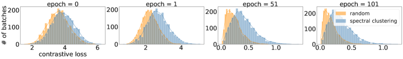
We provide additional results comparing the mini-batch counts of two batch selection algorithms: the proposed SC method and random batch selection. The mini-batch counts are based on the mini-batch contrastive loss con(𝑼,𝑽){\mathcal{L}}^{\operatorname{con}}({\bm{U}}_{{\mathcal{B}}},{\bm{V}}_{{\mathcal{B}}}). We measure mini-batch losses from ResNet-18 models trained on CIFAR-100 using the gradient descent algorithm with different batch selection methods: (i) SGD (Algo. 5), (ii) OSGD (Algo. 7), and (iii) the SC method (Algo. 3). Fig. 5 illustrates histograms of mini-batch counts for N/BN/B mini-batches, where N=50000N=50000 and B=20B=20. The results show that mini-batches generated through the proposed spectral clustering method tend to contain a higher proportion of large loss values when compared to the random batch selection, regardless of the pre-trained models used.

Refer to caption
Refer to caption
Refer to caption
Figure 5: Histograms of mini-batch counts for N/BN/B mini-batches, for the contrastive loss measured from ResNet-18 models trained on CIFAR-100 using different batch selection methods: (i) SGD (Top), (ii) OSGD (Middle), (iii) SC method (Bottom), where NN=50,000 and BB=20. Each column of plots is derived from a distinct training epoch. Here we compare two batch selection methods: (i) randomly shuffling NN samples and partition them into N/BN/B mini-batches of size BB, (ii) the proposed SC method given in Algo. 1. The histograms show that mini-batches generated through the proposed spectral clustering method tend to contain a higher proportion of large loss values when compared to random batch selection, regardless of the pre-trained models used.

D.2 Synthetic Dataset

With the settings from Sec. 6.1, where each column of embedding matrices 𝑼,𝑽{\bm{U}},{\bm{V}} is initialized as a multivariate normal vector and then normalized as 𝒖i=𝒗i=1\lVert{\bm{u}}_{i}\rVert=\lVert{\bm{v}}_{i}\rVert=1, for all ii, we provide the results for N{4,16}N\in\{4,16\} and d=2Nd=2N or d=N/2d=N/2. Fig. 6 and  7 show the results for N=4N=4 and N=16N=16, respectively. We additionally present the results for theoretically unproven cases, specifically for N=8N=8 and d{3,5}d\in\{3,5\} (see Fig. 8). The results provide empirical evidence that all combinations of mini-batches leads to the optimal solution of full-batch minimization for the theoretically unproven cases.

d=2Nd=2N Refer to captionRefer to captionRefer to captionRefer to captionRefer to caption

d=N/2d=N/2

Refer to caption
(a) solutions
Refer to caption
(b) full-batch
Refer to caption
(c) (NB){N\choose B}-all
Refer to caption
(d) (NB){N\choose B}-sub
Refer to caption
(e) norm differences
Figure 6: Heatmap of N×NN\times N matrix visualizing the resulting values from the same settings with Fig 4 except N=4N=4.

d=2Nd=2N Refer to captionRefer to captionRefer to captionRefer to captionRefer to caption

d=N/2d=N/2

Refer to caption
(a) solutions
Refer to caption
(b) full-batch
Refer to caption
(c) (NB){N\choose B}-all
Refer to caption
(d) (NB){N\choose B}-sub
Refer to caption
(e) norm differences
Figure 7: Heatmap of N×NN\times N matrix visualizing the resulting values from the same settings with Fig 4 except N=16N=16.

d=3d=3 Refer to captionRefer to captionRefer to caption

d=5d=5

Refer to caption
(a) full-batch
Refer to caption
(b) (NB){N\choose B}-all
Refer to caption
(c) (NB){N\choose B}-sub
Figure 8: Theoretically unproven setting. Heatmap of N×NN\times N matrix when N=8N=8 and d<N1d<N-1.

D.3 Real Datasets

To demonstrate the practical effectiveness of the proposed SC method, we consider a setting where embeddings are learned by a parameterized encoder. We employ two widely recognized uni-modal mini-batch contrastive learning algorithms: SimCLR [9] and SogCLR [68], and integrate different batch selection methods from: (i) SGD (algo. 5), (ii) OSGD (algo. 7), (iii) SC (algo. 3) into these frameworks. We compare the pre-trained models’ performances in the retrieval downstream tasks on the corrupted and the original datasets.

We conduct the mini-batch contrastive learning with the mini-batch size B=32B=32 using ResNet18-based encoders on CIFAR-100 and Tiny ImageNet datasets. All learning is executed on a single NVIDIA A100 GPU. The training code and hyperparameters are based on the official codebase of SogCLR333https://github.com/Optimization-AI/SogCLR [68]. We use LARS optimizer[67] with the momentum of 0.90.9 and the weight decay of 10610^{-6}. We utilize the learning rate scheduler which starts with a warm-up phase in the initial 10 epochs, during which the learning rate increases linearly to the maximum value ηmax=0.075B\eta_{\max}=0.075\sqrt{B}. After this warm-up stage, we employ a cosine annealing (half-cycle) schedule for the remaining epochs. For OSGD, we employ k=1500k=1500, q=150q=150. To expedite batch selection in the proposed SC, we begin by randomly partitioning NN positive pairs into kBkB-sized clusters, using k=40k=40. We then apply the SC method to each kBkB cluster to generate kk mini-batches, resulting in a total of k×(N/kB)=N/Bk\times(N/kB)=N/B mini-batches. We train models for a total of 100 epochs.

Table 2 presents the top-1 retrieval accuracy on CIFAR-100 and Tiny ImageNet. We measure validation retrieval performance on the true as well as corrupted datasets. The retrieval task is defined to be finding the positive pair image of a given image among all pairs (the number of images of the validation dataset).

Table 2: Top-1 retrieval accuracy on CIFAR-100 (or Tiny ImageNet), when each algorithm uses CIFAR-100 (or Tiny ImageNet) to pretrain ResNet-18 with SimCLR and SogCLR objective. SC algorithm proposed in Sec. 5.3 outperforms existing baselines.
Image Retrieval
CIFAR-100 Tiny ImageNet
SimCLR SogCLR SimCLR SogCLR
SGD 46.91% 12.34% 57.88% 16.70%
OSGD 47.55% 13.88% 59.34% 20.43%
SC 56.67%\bm{56.67}\% 47.42%\bm{47.42}\% 68.07%\bm{68.07}\% 54.20%\bm{54.20}\%

We also consider the retrieval task under a harder setting, where the various corruptions are applied per image so that we can consider a set of corrupted images as a hard negative samples. Table 1 presents the top-1 retrieval accuracy results on CIFAR-100-C and Tiny ImageNet-C, the corrupted datasets [23] designed for robustness evaluation. CIFAR-100-C (Tiny ImageNet-C) has the same images as CIFAR-100 (Tiny ImageNet), but these images have been altered by 19 (15) different types of corruption (e.g., image noise, blur, etc.). Each type of corruption has five severity levels. We utilize images corrupted at severity level 1. These images tend to be more similar to each other than those corrupted at higher severity levels, which consequently makes it more challenging to retrieve positive pairs among other images. To perform the retrieval task, we follow the following procedures: (i) We apply two distinct augmentations to each image to generate positive pairs; (ii) We extract embedding features from the augmented images by employing the pre-trained models; (iii) we identify the pair image of the given augmented image among augmentations of 19 (15) corrupted images with the cosine similarity of embedding vectors. This process is iterated across 1010K CIFAR-100 images (1010K Tiny-ImageNet images). The top-1 accuracy measures a percentage of retrieved images that match its positive pair image, where each pair contains two different modality stemming from a single image.