Minimal area conics in the elliptic plane

Matthias. J. Weber and Hans-Peter Schröcker Matthias. J. Weber, Hans-Peter Schröcker, Unit Geometry and CAD, University Innsbruck, Technikerstraße 13, 6020 Innsbruck, Austria

(Date: September 6, 2025)

Abstract.

We prove some uniqueness results for conics of minimal area that enclose a compact, full-dimensional subset of the elliptic plane. The minimal enclosing conic is unique if its center or axes are prescribed. Moreover, we provide sufficient conditions on the enclosed set that guarantee uniqueness without restrictions on the enclosing conics. Similar results are formulated for minimal enclosing conics of line sets as well.

Key words and phrases:

Minimal conic, sphero-conic, spherical ellipse, covering cone, elliptic geometry, spherical geometry, enclosing conic, uniqueness

2010 Mathematics Subject Classification:

52A40; 52A55, 51M10

1. Introduction

It is well know that every compact subset $F$ of the Euclidean plane with inner points can be enclosed by a unique ellipse of minimal area. More generally, every compact subset $F$ of $d$ -dimensional Euclidean space with inner points defines a unique enclosing ellipsoid of minimal volume (see [2, 3] for the case $d=2$ and [8, 4] for general $d$ ).

These uniqueness results are generally considered as “easy”. The reason for the existence of simple proofs are illuminated by recent publications of the authors [15, 16]. We showed that numerous uniqueness results in Euclidean spaces are a consequence of a simple convexity property of the function that measures the ellipsoid’s size. Most notably, minimal enclosing ellipsoids with respect to quermass integrals are unique (see also [6, 7]).

In the present article we establish first uniqueness results in the elliptic plane. We provide sufficient conditions on the enclosed set $F$ that guarantee uniqueness of the minimal enclosing conic. To the best of our knowledge, these are the first uniqueness results in a non-Euclidean geometry. This is maybe the case because our uniqueness results are not easy in the sense described above. While uniqueness in the co-axial and concentric case can still be deduced from a convexity property of the area function, uniqueness in the general case requires extra work. The necessary calculations are rather involved and constitute the largest part of this article.

We mostly use the spherical model of the elliptic plane. It is easily obtained from the bundle model whose “points” are the one-dimensional subspaces of the vector space $\mathbb{R}^{3}$ . The distance of two points in the bundle model is defined as the Euclidean angle between lines and is a bi-valued function. The straight lines in the bundle model are the two-dimensional subspaces. Their angle is the usual Euclidean angle.

In this setting, computational aspects of the minimal circular cone problem (where uniqueness is elementary) have already attracted the attention of applied mathematicians [12, 1]. We believe that the applications mentioned in [1] could profit from using minimal enclosing conics (or cones of second degree) instead of circles (or right circular cones).

The spherical model of the elliptic plane is obtained by intersecting the bundle model with the unit sphere $S^{2}$ . The metric is inherited from the ambient Euclidean space and the only difference to spherical geometry is the identification of antipodal points. This is merely a technical issue so that our uniqueness results can also be formulated for sphero-conics.

We continue this article by an introduction to conics in the elliptic plane. In Section 3 we derive some convexity properties of their area function which are used in Section 4.1 for proving uniqueness in the co-axial and concentric case. The general uniqueness result is presented in Section 4.2. In Section 5 we derive uniqueness results for minimal enclosing conics of line-sets, analogous to those of [14]. The duality between points and lines in the elliptic plane makes them simple corollaries. Most auxiliary results are collected in an appendix.

2. Preliminaries

A conic $C$ in the spherical model of the elliptic plane is the intersection of the unit sphere $S^{2}$ with a quadratic cone whose vertex is the center of $S^{2}$ :

(1)

C=\{x\in S^{2}\colon x^{\mathrm{T}}\cdot M\cdot x=0\},

where $M\in\mathbb{R}^{3\times 3}$ is an indefinite symmetric matrix of full rank. Since proportional matrices describe the same conic, it is no loss of generality to assume that $M$ has eigenvalues $\nu_{1}\geq\nu_{2}>0$ and $\nu_{3}=-1$ . Then the interior of the conic $C$ consists of all points $x$ that fulfill the inequality $x^{\mathrm{T}}\cdot M\cdot x<0$ .

Refer to caption — Figure 1. Conic as intersection of $S^{2}$ with a quadratic cone

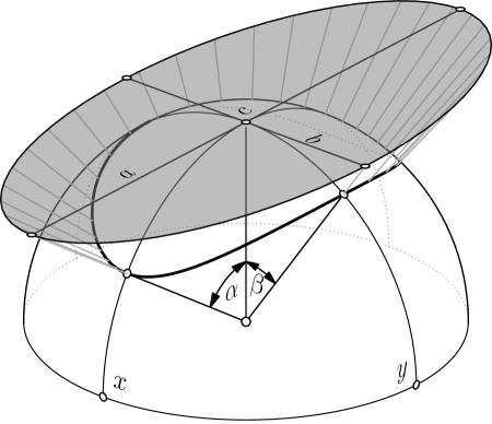
The transformation group of elliptic geometry is the rotation group $\mathrm{SO}(3)$ . Thus, the matrix $M$ has the normal form

(2)

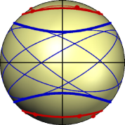
M=\operatorname{diag}(\nu_{1},\nu_{2},-1)=\operatorname{diag}(b^{-2},a^{-2},-1)

where $a=\nu_{2}^{-1/2}$ , $b=\nu_{1}^{-1/2}$ . The values $\alpha=\arctan a$ and $\beta=\arctan b$ are the conic’s semi-axis lengths (Figure 1).

Generally, the three points $x=(1,0,0)^{\mathrm{T}}$ , $y=(0,1,0)^{\mathrm{T}}$ , and $c=(0,0,1)^{\mathrm{T}}$ are called the centers of $C$ . Any line through one of them is a diameter since its intersection points with the conic are at equal (possibly complex) distance to the center. Among the three centers the point $c$ is distinguished by the fact that it lies in the interior of $C$ . It has also a special meaning in the context of minimal enclosing conics so that we use the word center exclusively for the point $c$ . The three lines spanned by any two of the points $x$ , $y$ , and $c$ are lines of symmetry and are often called axes. We reserve this term for the two lines $X=c\vee x$ and $Y=c\vee y$ . If $\alpha>\beta$ , we call $X$ the major axis and $Y$ the minor axis.

Note that elliptic geometry does not distinguish between different types of regular conics apart from circles and non-circular (general) conics. Indeed, the point set (1) satisfies the well-known focal definitions of both, ellipses and hyperbolas. This is possible because the distance in the elliptic plane is bi-valued.

If $M$ is not in normal form, semi-axis lengths, center, and axes can be obtained from the eigenvalues and eigenvectors of $M$ . Denote the vector of eigenvalues of $M$ , arranged in decreasing order, by $e(M)$ ,

(3)

e(M)=(\nu_{1},\nu_{2},\nu_{3})^{\mathrm{T}},\quad\text{where}\quad\nu_{1}\geq\nu_{2}>0\quad\text{and}\quad\nu_{3}<0,

and the corresponding eigenvectors by $y$ , $x$ , and $c$ . The function

(4)

w\colon(\nu_{1},\nu_{2},\nu_{3})^{\mathrm{T}}\mapsto(a,b)^{\mathrm{T}}=\Bigl{(}\sqrt{-\frac{\nu_{3}}{\nu_{2}}},\sqrt{-\frac{\nu_{3}}{\nu_{1}}}\Bigr{)}^{\mathrm{T}},

computes the tangents $a=\tan\alpha$ and $b=\tan\beta$ of the semi-axis lengths $\alpha$ and $\beta$ . The vector $c$ points to the center of $C$ . If $\nu_{1}>\nu_{2}$ , the conic is not a circle, the major axis exists and is incident with $x$ .

3. The area of a conic in the elliptic plane

Now we derive some properties of the area function of conics in the elliptic plane. The surface area of $C$ is a strictly monotone increasing function of $\alpha$ and $\beta$ . For our purpose it is more convenient to view it as a strictly monotone decreasing function of the variables $-\nu_{1}/\nu_{3}$ and $-\nu_{2}/\nu_{3}$ .

3.1. The area function.

We compute the area for the normal form (2) of the matrix $M$ . The upper half of the unit sphere $S^{2}$ can be parametrized as

(5)

S^{2}\colon\begin{pmatrix}\cos\varphi\cos\vartheta\\ \sin\varphi\cos\vartheta\\ \sin\vartheta\end{pmatrix},\quad\varphi\in[-\pi,\pi],\ \vartheta\in\bigl{[}0,\frac{\pi}{2}\bigr{]}.

The points inside $C$ belong to parameter values $(\varphi,\vartheta)$ related by

(6)

|\vartheta|>\vartheta_{0}=\arcsin\biggl{(}\sqrt{\frac{a^{2}\sin^{2}\varphi+b^{2}\cos^{2}\varphi}{a^{2}b^{2}+a^{2}\sin^{2}\varphi+b^{2}\cos^{2}\varphi}}\biggr{)}.

By integrating the area element $\cos\vartheta\,\operatorname{d\!}\vartheta\wedge\operatorname{d\!}\varphi$ of (5) we obtain the area of the conic $C$ as

(7)

\operatorname{area}(C)=\operatorname{area}(a,b)=\int_{-\pi}^{\pi}\int_{\vartheta_{o}}^{\pi/2}\cos\vartheta\operatorname{d\!}\vartheta\operatorname{d\!}\varphi=\int_{-\pi}^{\pi}1-\sin\vartheta_{0}\operatorname{d\!}\varphi\\ =2\pi-\int_{-\pi}^{\pi}\sqrt{\frac{a^{2}\sin^{2}\varphi+b^{2}\cos^{2}\varphi}{a^{2}b^{2}+a^{2}\sin^{2}\varphi+b^{2}\cos^{2}\varphi}}\operatorname{d\!}\varphi.

The integral representation (7) is perfectly suitable for our purposes so that we refrain from expressing the area in terms of elliptic integrals. Substituting $a^{2}=-\nu_{3}/\nu_{2}$ and $b^{2}=-\nu_{3}/\nu_{1}$ into (7) we obtain the area in terms of the eigenvalues of the matrix $M$ :

(8)

\operatorname{area}(C)=\operatorname{area}(\nu_{1},\nu_{2},\nu_{3})=2\pi-\int_{-\pi}^{\pi}\sqrt{\frac{\nu_{1}\sin^{2}\varphi+\nu_{2}\cos^{2}\varphi}{-\nu_{3}+\nu_{1}\sin^{2}\varphi+\nu_{2}\cos^{2}\varphi}}\operatorname{d\!}\varphi.

The matrix $M$ is determined by the conic $C$ only up to a scalar factor. Thus, we may normalize it such that $\nu_{3}=-1$ . Then the area becomes

(9)

\operatorname{area}(C)=\operatorname{area}(\nu_{1},\nu_{2})=2\pi-\int_{-\pi}^{\pi}\sqrt{\frac{\nu_{1}\sin^{2}\varphi+\nu_{2}\cos^{2}\varphi}{1+\nu_{1}\sin^{2}\varphi+\nu_{2}\cos^{2}\varphi}}\operatorname{d\!}\varphi.

3.2. Convexity of the area function

We prove that the function (9) is strictly convex for $\nu_{1}$ , $\nu_{2}>0$ . The standard arguments of [15, 16] then imply uniqueness of the minimal enclosing conic among all conics with prescribed axes or prescribed center. These proofs are given later, in Section 4.

Lemma 1.

The area function (9) is strictly convex.

Proof.

We show that the Hessian $H$ of (9) is positive definite, that is, all its principal minors are positive. The upper left entry of $H$ equals

(10)

\mathinner{\dfrac{\partial{{}^{2}}\operatorname{area}}{\partial{\nu_{1}^{2}}}}=\frac{1}{4}\int_{-\pi}^{\pi}J\sin^{4}\varphi\operatorname{d\!}\varphi,

where

(11)

J=\frac{1+4\nu_{1}\sin^{2}\varphi+4\nu_{2}\cos^{2}\varphi}{(\nu_{1}\sin^{2}\varphi+\nu_{2}\cos^{2}\varphi)^{3/2}(1+\nu_{1}\sin^{2}\varphi+\nu_{2}\cos^{2}\varphi)^{5/2}}.

Clearly, the integral (10) is strictly positive. The determinant of $H$ equals

(12)

\mathinner{\dfrac{\partial{{}^{2}}\operatorname{area}}{\partial{\nu_{1}^{2}}}}\mathinner{\dfrac{\partial{{}^{2}}\operatorname{area}}{\partial{\nu_{2}^{2}}}}-\biggl{(}\mathinner{\dfrac{\partial{}\operatorname{area}}{\partial{\nu_{1}}\partial{\nu_{2}}}}\biggr{)}^{2}=\\ \frac{1}{16}\int_{-\pi}^{\pi}J\sin^{4}\varphi\operatorname{d\!}\varphi\cdot\int_{-\pi}^{\pi}J\cos^{4}\varphi\operatorname{d\!}\varphi-\frac{1}{16}\Bigl{(}\int_{-\pi}^{\pi}J\sin^{2}\varphi\cos^{2}\varphi\operatorname{d\!}\varphi\Bigr{)}^{2}.

By the Schwarz inequality we have

(13)

\sqrt{\int_{-\pi}^{\pi}\bigl{(}\sqrt{J}\sin^{2}\varphi\bigr{)}^{2}\operatorname{d\!}\varphi}\cdot\sqrt{\int_{-\pi}^{\pi}\bigl{(}\sqrt{J}\cos^{2}\varphi\bigr{)}^{2}\operatorname{d\!}\varphi}\geq\int_{-\pi}^{\pi}J\sin^{2}\varphi\cos^{2}\varphi\operatorname{d\!}\varphi,

with equality precisely if the integrands on the left are proportional. Since this is not the case, (12) is strictly positive as well. Hence, the Hessian of $H$ is positive definite and $\operatorname{area}(\nu_{1},\nu_{2})$ is strictly convex. ∎

4. Uniqueness results

We are aware of two essentially different methods for proving uniqueness of minimal circumscribed (or maximal inscribed) conics. One may consider the problem as an optimization task and derive sufficient conditions for the existence of a unique minimizer or maximizer. This is the approach of [8, 9, 10]. The second method of proof is indirect. Assuming existence of two minimizers (or maximizers in case of inscribed conics) $C_{0}$ and $C_{1}$ one shows existence of a further circumscribing (or inscribed) conic $C$ of smaller (or larger) size. This idea or variants of it can be found in [4, 11, 7, 15, 16]. In this article, we adopt it as well. In our setup, the equation of the conic $C$ is found as a convex combination of the respective equations of $C_{0}$ and $C_{1}$ :

Definition 2 (in-between conic).

Let $C_{0}$ and $C_{1}$ be two conics

(14)

C_{i}=\{x\in S^{2}\colon x^{\mathrm{T}}\cdot M_{i}\cdot x=0\},\quad i=0,1

such that the matrices $M_{i}$ are indefinite and have precisely one negative eigenvalue $\nu_{3,i}=-1$ . For $\lambda\in(0,1)$ we define the in-between conic $C_{\lambda}$ to $C_{0}$ and $C_{1}$ as

(15)

C_{\lambda}=\{x\in S^{2}\colon x^{\mathrm{T}}\cdot M_{\lambda}\cdot x=0\},

with

(16)

M_{\lambda}=(1-\lambda)M_{0}+\lambda M_{1}.

We also use the symbolic notation $C_{\lambda}=(1-\lambda)C_{0}+\lambda C_{1}$ . As long as $C_{0}$ and $C_{1}$ have a common interior, $C_{\lambda}$ is a non-degenerate conic whose interior contains the common interior of $C_{0}$ and $C_{1}$ . In general, the unique negative eigenvalue of $M_{\lambda}$ is different from $-1$ (in fact larger than $-1$ as the smallest eigenvalue is a concave function of $\lambda$ ). This hinders the usage of (9) and accounts for most difficulties in the general proof of uniqueness. If the conics $C_{0}$ and $C_{1}$ have the same axes or the same center the situation is much simpler.

4.1. Coaxial and concentric conics

We call a subset $F$ of the elliptic plane bounded, if it is contained in a circle and we call it full-dimensional if it is not contained in a line. In this section we prove that any bounded, compact and full-dimensional subset $F$ of the elliptic plane can be enclosed by a unique conic of minimal area with prescribed axes or center. The proofs of uniqueness are simple and follow the general scheme outlined in [15]. Nonetheless, the concentric case constitutes the basis for the much deeper general uniqueness result in Section 4.2.

Theorem 3.

Let $F$ be a bounded, compact and full-dimensional subset of the elliptic plane. Among all conics with two given axes that contain $F$ there exists exactly one of minimal area.

Proof.

Existence is a direct consequence of compactness and boundedness of $F$ and continuity of the area function. In order to show uniqueness, assume $C_{0}$ and $C_{1}$ are two minimal conics with prescribed axes and circumscribing $F$ . Because $F$ is full-dimensional, both $C_{0}$ and $C_{1}$ are not degenerate. In a suitable coordinate frame we can describe them by diagonal matrices

(17)

M_{i}=\operatorname{diag}(\nu_{i,1},\nu_{i,2},-1),\quad\nu_{i,1}\geq\nu_{i,2}>0,\quad i=0,1.

The in-between conic $C_{\lambda}$ is then given by

(18)

M_{\lambda}=\operatorname{diag}\bigl{(}(1-\lambda)\nu_{0,1}+\lambda\nu_{1,1},\ (1-\lambda)\nu_{0,2}+\lambda\nu_{1,2},-1\bigr{)}.

Because the area function (9) is strictly convex we have

(19)

\operatorname{area}\circ\,w\circ e(M_{\lambda})<(1-\lambda)\operatorname{area}\circ\,w\circ e(M_{0})+\lambda\operatorname{area}\circ\,w\circ e(M_{1})

(the functions $e$ and $w$ are defined in (3) and (4), respectively). Hence, the area of $C_{\lambda}$ is strictly smaller than that of $C_{0}$ and $C_{1}$ — a contradiction to the assumed minimality of $C_{0}$ and $C_{1}$ . ∎

Uniqueness of minimal enclosing conics among all conics with prescribed center follows again from the strict convexity of (9) and

Proposition 4 (Davis’ Convexity Theorem).

A convex, lower semi-continuous and symmetric function $f$ of the eigenvalues of a symmetric matrix is (essentially strict) convex on the set of symmetric matrices if and only if its restriction to the set of diagonal matrices is (essentially strict) convex.

A proof for the convex case is given in [5]. The extension to essentially strict convexity is due to [13]. We skip the technicalities related to the precise definition of “essentially strict convexity”. All prerequisites are met in our case and all necessary conclusions can be drawn.

Theorem 5.

Let $F$ be a bounded, compact and full-dimensional subset of the elliptic plane. Among all conics with given center that contain $F$ there exists exactly one of minimal area.

Proof.

The proof is similar to that of Theorem 3. Instead of the diagonal matrices (17) and (18) we have matrices of the shape

(20)

M_{i}=\begin{pmatrix}\star&\star&0\\ \star&\star&0\\ 0&0&-1\end{pmatrix},\quad i\in\{0,1,\lambda\}.

Davis’ Convexity Theorem guarantees strict convexity of the function $\operatorname{area}\circ\,w\circ e$ on the space of matrices of type (20). ∎

4.2. The general case

Now we come to the general case. Here, we cannot make use of Davis’ Convexity Theorem since the negative eigenvalue of the matrix $M_{\lambda}$ is different from $-1$ and the area can no longer be regarded as convex function in the positive eigenvalues of $M_{\lambda}$ . In fact, there exist situations where

(21)

\operatorname{area}(C_{\lambda})>\operatorname{area}(C_{0})=\operatorname{area}(C_{1})

for all in-between conics $C_{\lambda}$ . We present an example of this:

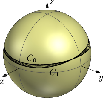
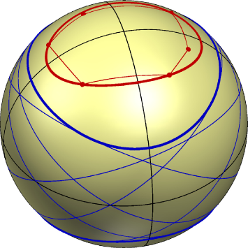
Example 6.

Let $C_{0}$ and $C_{1}$ be two congruent conics described by

(22)

\textstyle M_{0}=\operatorname{diag}(\frac{1}{16},\frac{1}{36},-1)\quad\text{and}\quad M_{1}=R_{1}\cdot R_{2}\cdot R_{3}\cdot M_{0}\cdot(R_{1}\cdot R_{2}\cdot R_{3})^{\mathrm{T}}

where $R_{1}$ , $R_{2}$ , $R_{3}$ are the rotation matrices

(23)

\textstyle R_{1}=\left(\begin{smallmatrix}1&0&0\\ 0&\cos\frac{\pi}{60}&-\sin\frac{\pi}{60}\\ 0&\sin\frac{\pi}{60}&\phantom{-}\cos\frac{\pi}{60}\end{smallmatrix}\right),\ R_{2}=\left(\begin{smallmatrix}\cos\frac{\pi}{36}&0&-\sin\frac{\pi}{36}\\ 0&1&0\\ \sin\frac{\pi}{36}&0&\phantom{-}\cos\frac{\pi}{36}\end{smallmatrix}\right),\ R_{3}=\left(\begin{smallmatrix}\cos\frac{\pi}{6}&-\sin\frac{\pi}{6}&0\\ \sin\frac{\pi}{6}&\phantom{-}\cos\frac{\pi}{6}&0\\ 0&0&1\end{smallmatrix}\right).

The two conics are congruent (hence of equal area) and have a non-empty common interior. Figure 3, left, displays them together with a few in-between conics. Figure 3, right, shows a plot of the area function of $C_{\lambda}$ on the interval $(0,1)$ . We see that the area of any in-between conic is larger than $\operatorname{area}C_{0}=\operatorname{area}C_{1}$ .

Example 6 illustrates the difficulties we have to expect when proving uniqueness results for non concentric conics in the elliptic plane. Additional assumptions on the enclosed set $F$ are inevitable at least for our method of proof which is based on in-between conics of Definition 2.

The behaviour illustrated in Example 6 is in contrast to the situation in the Euclidean plane, where a convexity property of the size function similar to Lemma 1 guarantees that the in-between ellipsoids $C_{\lambda}$ can be translated so that they are completely contained in $C_{0}$ or $C_{1}$ (the “Translation Lemma 6” of [15]). In particular, the size of every in-between ellipsoid is strictly smaller than the size of $C_{0}$ and $C_{1}$ (for any reasonable size function). An important observation is that the conics $C_{0}$ and $C_{1}$ in Example 6 are rather large and “far away” from a pair of Euclidean conics. Thus, one might hope that uniqueness via in-between conics can be shown for sufficiently small conics. This is indeed the case. A precise formulation is given below. It requires an auxiliary result:

Lemma 7.

The function

(24)

J(v)=\int_{0}^{w}\frac{1+v-3t^{2}}{\sqrt{1-t^{2}}}\operatorname{d\!}t+\int_{w}^{1}\frac{(1+v-3t^{2})\sqrt{1+v}}{\sqrt{1-t^{2}}\sqrt{1+v-t^{2}}}\operatorname{d\!}t\quad\text{with}\quad w=\sqrt{\frac{1+v}{3}}

is strictly monotone increasing in $[0,2]$ . In particular, it has precisely one zero $v_{0}\approx 0.685935$ in this interval.

Proof.

Denote the first integral in (24) by $J_{1}(v)$ and the second by $J_{2}(v)$ . Clearly, $J_{1}(v)$ is strictly monotone increasing in $v$ because the integrand and the upper integration bound are strictly monotone increasing. The integrand of $J_{2}(v)$ is negative. Thus, increasing the lower integration bound $w$ will also increase the integral. Moreover, the second integrand is strictly monotone increasing in $v$ as well. In order to see this, we compute its first derivative with respect to $v$ :

(25)

\frac{2v^{2}+(4-3t^{2})v+3t^{4}-3t^{2}+2}{2\sqrt{1-t^{2}}\sqrt{1+v}\;(1+v-t^{2})^{3/2}}.

The denominator is positive, the numerator is strictly monotone increasing in $v$ and, for $v=0$ , attains the positive value $3t^{4}-3t^{2}+2$ . Thus, the derivative is positive. This implies that the integrand of $J_{2}$ is strictly monotone increasing and the same is true for the function $J$ defined in (24). ∎

Theorem 8.

Denote the unique zero of $\eqref{eq:24}$ in $[0,2]$ by $v_{0}$ and let $\mathrm{R}=\arctan(v_{0}^{-1/2})$ . The enclosing conic of minimal area of a compact subset $F$ of the elliptic plane is unique if the following two conditions are met:

(1)

The elliptic convex hull of $F$ contains a circle of radius $\varrho>0$ . In particular, $F$ is full-dimensional.
(2)

There exists an enclosing conic of $F$ whose area is less than $\operatorname{area}(\mathrm{R},\varrho)$ , computed by means of Equation (7).

Note that the requirements of this theorem imply restrictions on the set $F$ and all candidates for enclosing conics of minimal area:

•

The diameter of $F$ is less than $\mathrm{R}$ , that is, $F$ is bounded by a fixed value derived from the function $J(v)$ .
•

Any enclosing conic has a minor semi-axis lengths $\beta\geq\varrho$ and any minimal enclosing conic has a major semi-axis length $\alpha<\mathrm{R}$ . In other words, if we insert the value $v=1/\tan^{2}\alpha$ into the function $J(v)$ , the result is positive.

The basic idea of the proof is not different from the proofs of Theorems 3 and 5 but the details are more involved. Existence of the minimal enclosing conic follows from the usual compactness argument. In order to prove uniqueness, we assume existence of two conics $C_{0}$ and $C_{1}$ of minimal area that contain $F$ . Note that their minor semi-axis length is not smaller than $\varrho$ and their major semi-axis lengths is smaller than $\mathrm{R}$ . We show existence of an in-between conic $C_{\lambda}$ such that $\operatorname{area}(C_{\lambda})<\operatorname{area}(C_{0})=\operatorname{area}(C_{1})$ . This we do by proving that $\operatorname{area}(C_{\lambda})$ is strictly monotone decreasing in the vicinity of $\lambda=0$ (possibly after interchanging $C_{0}$ and $C_{1}$ ). Thus, we obtain a contradiction to the assumed minimality of $C_{0}$ and $C_{1}$ . In order to show that $\operatorname{area}(C_{\lambda})$ is strictly monotone decreasing in the vicinity of $\lambda=0$ , we compare the derivative of the area function with respect to $\lambda$ to the derivative of the area function in a suitably constructed case with concentric conics (Lemma 9). The details of this proof span until the end of this section. Auxiliary results of technical nature are proved in the appendix.

4.2.1. Assumptions on the semi-axis lengths

For $i=0$ , $1$ we denote the matrix describing the conic $C_{i}$ by $M_{i}$ . Its eigenvalues are $\nu_{i,1}\geq\nu_{i,2}>0$ and $\nu_{i,3}=-1$ . It is no loss of generality to make a few assumptions on these values:

If $\nu_{0,1}=\nu_{0,2}$ and $\nu_{1,1}=\nu_{1,2}$ , equality of areas of $C_{0}$ and $C_{1}$ implies $\nu_{0,1}=\nu_{0,2}=\nu_{1,1}=\nu_{1,2}$ . In this case both conics are congruent circles with two real intersection points $s_{1}$ , $s_{2}$ . There exists a circle with $s_{1}$ and $s_{2}$ as end-points of a diameter which also contains the common interior of $C_{0}$ and $C_{1}$ . It is smaller than $C_{0}$ and $C_{1}$ and thus contradicts the assumed minimality of these conics. Henceforth, we exclude equality of all four positive eigenvalues of $M_{0}$ and $M_{1}$ . Then equality of areas of $C_{0}$ and $C_{1}$ implies that these eigenvalues can be nested (possibly after interchanging $C_{0}$ and $C_{1}$ ) according to

(26)

\nu_{0,1}>\nu_{1,1}\geq\nu_{1,2}>\nu_{0,2}.

4.2.2. Derivative of the area function

As already mentioned, a contradiction to the assumed minimality of $C_{0}$ and $C_{1}$ arises if we can show that

(27)

\dfrac{\operatorname{d\!}{}\operatorname{area}(C_{\lambda})}{\operatorname{d\!}{\lambda}}\Big{|}_{\lambda=0}<0.

The advantage of this “local” approach is that the derivative (27) can be computed from the derivatives of the eigenvalues $\nu_{i,1}$ and $\nu_{i,2}$ with respect to $\lambda$ and that these derivatives do not require explicit expressions of the eigenvalues as functions of $\lambda$ .

We assume that $C_{0}$ is of the normal form (2) and $C_{1}$ is obtained from a conic in this normal form by a rotation about an axis through the center of $S^{2}$ , that is,

(28)

M_{0}=\begin{pmatrix}\nu_{0,1}&0&0\\ 0&\nu_{0,2}&0\\ 0&0&-1\end{pmatrix},\quad M_{1}=Q\cdot\begin{pmatrix}\nu_{1,1}&0&0\\ 0&\nu_{1,2}&0\\ 0&0&-1\end{pmatrix}\cdot Q^{-1},

with the rotation matrix

(29)

Q=\begin{pmatrix}q_{0}^{2}+q_{1}^{2}-q_{2}^{2}-q_{3}^{2}&2(q_{1}q_{2}-q_{0}q_{3})&2(q_{1}q_{3}+q_{0}q_{2})\\ 2(q_{1}q_{2}+q_{0}q_{3})&q_{0}^{2}-q_{1}^{2}+q_{2}^{2}-q_{3}^{2}&2(q_{2}q_{3}-q_{0}q_{1})\\ 2(q_{1}q_{3}-q_{0}q_{2})&2(q_{2}q_{3}+q_{0}q_{1})&q_{0}^{2}-q_{1}^{2}-q_{2}^{2}+q_{3}^{2}\end{pmatrix}

and $q_{0}^{2}+q_{1}^{2}+q_{2}^{2}+q_{3}^{2}=1$ . The rotation angle $\theta$ is given by $q_{0}=\cos 2\theta$ , the axis direction is $(q_{1},q_{2},q_{3})^{\mathrm{T}}$ . The matrix $M_{\lambda}$ of the in-between conic is computed according to (16). Its ordered eigenvalues $\nu_{1}(\lambda)\geq\nu_{2}(\lambda)\geq\nu_{3}(\lambda)$ are functions of $\lambda$ and in the vicinity of $\lambda=0$ we have $\nu_{1}(\lambda)>\nu_{2}(\lambda)>0>\nu_{3}(\lambda)$ . The eigenvalues are implicitly defined as roots of the characteristic polynomial $P(\lambda,\nu(\lambda))=\det(M_{\lambda}-\nu I_{3})$ of $M_{\lambda}$ , $I_{3}$ being the three by three identity matrix. We know the values of these roots for $\lambda=0$ :

(30)

\nu_{1}(0)=\nu_{0,1},\quad\nu_{2}(0)=\nu_{0,2},\quad\nu_{3}(0)=-1.

By implicit derivation we have

(31)

\mathinner{\dfrac{\operatorname{d\!}{}\nu_{i}}{\operatorname{d\!}{\lambda}}}(0)=-\frac{\dfrac{\partial{}P}{\partial{\lambda}}(0,\nu_{i}(0))}{\dfrac{\partial{}P}{\partial{\nu}}(0,\nu_{i}(0))},\quad i=1,2,3,

which gives us the derivatives of the three eigenvalues of $M_{\lambda}$ at $\lambda=0$ . Furthermore, we can compute

(32)

\mathinner{\dfrac{\partial{}\operatorname{area}(\nu_{0,1},\nu_{0,2},\nu_{0,3})}{\partial{\nu_{0,i}}}},\quad i=1,2,3

and, using the chain rule

(33)

\mathinner{\dfrac{\partial{}\operatorname{area}(C_{\lambda})}{\partial{\lambda}}}\Big{|}_{\lambda=0}=\mathinner{\dfrac{\partial{}\operatorname{area}}{\partial{\nu_{0,1}}}}\frac{\partial\nu_{\lambda,1}}{\partial\lambda}\Big{|}_{\lambda=0}+\mathinner{\dfrac{\partial{}\operatorname{area}}{\partial{\nu_{0,2}}}}\frac{\partial\nu_{\lambda,2}}{\partial\lambda}\Big{|}_{\lambda=0}+\mathinner{\dfrac{\partial{}\operatorname{area}}{\partial{\nu_{0,3}}}}\frac{\partial\nu_{\lambda,3}}{\partial\lambda}\Big{|}_{\lambda=0},

we find

(34)

\mathinner{\dfrac{\partial{}\operatorname{area}(C_{\lambda})}{\partial{\lambda}}}\Big{|}_{\lambda=0}=\\ -\frac{1}{2}\int_{-\pi}^{\pi}\frac{1}{N}\bigl{(}\sin^{2}\varphi(q_{1,1}^{2}\nu_{1,1}+q_{1,2}^{2}\nu_{1,2}-q_{1,3}^{2}+\nu_{0,1}(q_{3,1}^{2}\nu_{1,1}+q_{3,2}^{2}\nu_{1,2}-q_{3,3}^{2}))\\ +\cos^{2}\varphi(q_{2,1}^{2}\nu_{1,1}+q_{2,2}^{2}\nu_{1,2}-q_{2,3}^{2}+\nu_{0,2}(q_{3,1}^{2}\nu_{1,1}+q_{3,2}^{2}\nu_{1,2}-q_{3,3}^{2}))\bigr{)}\operatorname{d\!}\varphi,

where

(35)

N=(\nu_{0,1}\sin^{2}\varphi+\nu_{0,2}\cos^{2}\varphi)^{1/2}(1+\nu_{0,1}\sin^{2}\varphi+\nu_{0,2}\cos^{2}\varphi)^{3/2}

and $q_{i,j}$ are the entries of the rotation matrix (29). Equation (34) expresses the derivative of the area function with respect to $\lambda$ at $\lambda=0$ in terms of the two initially given conics $C_{0}$ and $C_{1}$ . It will be convenient to write (34) in terms of the first and second complete elliptic integrals

(36)

K(z)=\int_{0}^{1}\frac{1}{\sqrt{1-t^{2}}\sqrt{1-z^{2}t^{2}}}\operatorname{d\!}t\quad\text{and}\quad E(z)=\int_{0}^{1}\frac{\sqrt{1-z^{2}t^{2}}}{\sqrt{1-t^{2}}}\operatorname{d\!}t.

Since we will evaluate them only at

(37)

f=\sqrt{\frac{\nu_{0,1}-\nu_{0,2}}{\nu_{0,1}(1+\nu_{0,2})}},

we use the abbreviations $\bar{E}\mathrel{\mathop{\ordinarycolon}}=E(f)$ and $\bar{K}\mathrel{\mathop{\ordinarycolon}}=K(f)$ . By (26), $f$ is always real.

Substituting $x=\nu_{0,1}\sin^{2}\varphi+\nu_{0,2}\cos^{2}\varphi$ into (34) and noting that $(x-\nu_{0,1})(\nu_{0,2}-x)=(\nu_{0,1}-\nu_{0,2})^{2}\cos^{2}\varphi\sin^{2}\varphi$ we can express the derivative of the area function in terms of elliptic integrals:

(38)

\mathinner{\dfrac{\partial{}\operatorname{area}(C_{\lambda})}{\partial{\lambda}}}\Big{|}_{\lambda=0}=\frac{2}{\sqrt{\nu_{0,1}(1+\nu_{0,2})}(\nu_{0,1}-\nu_{0,2})(1+\nu_{0,1})}\\ \bigl{(}(1+\nu_{0,1})(-\nu_{0,1}(q_{2,1}^{2}\nu_{1,1}+q_{2,2}^{2}\nu_{1,2}-q_{2,3}^{2})+\nu_{0,2}(q_{1,1}^{2}\nu_{1,1}+q_{1,2}^{2}\nu_{1,2}-q_{1,3}^{2}))\bar{K}\\ -\nu_{0,1}(\nu_{0,1}(q_{3,1}^{2}\nu_{1,1}+q_{3,2}^{2}\nu_{1,2}-q_{3,3}^{2}-q_{2,1}^{2}\nu_{1,1}-q_{2,2}^{2}\nu_{1,2}+q_{2,3}^{2})\\ +\nu_{0,2}(-q_{3,1}^{2}\nu_{1,1}-q_{3,2}^{2}\nu_{1,2}+q_{3,3}^{2}+q_{1,1}^{2}\nu_{1,1}+q_{1,2}^{2}\nu_{1,2}-q_{1,3}^{2})\\ +q_{1,1}^{2}\nu_{1,1}+q_{1,2}^{2}\nu_{1,2}-q_{1,3}^{2}-q_{2,1}^{2}\nu_{1,1}-q_{2,2}^{2}\nu_{1,2}+q_{2,3}^{2})\bar{E}\bigr{)}.

4.2.3. The half-turn lemma

From the proof of Theorem 5 we already know that (38) is negative if $C_{0}$ and $C_{1}$ are concentric. We show negativity in the general case by comparison with a concentric situation. This is a direct consequence of the “Half-Turn Lemma” below. The basic idea already occurred in [15] in form of a “Translation Lemma”.

Lemma 9 (Half-Turn Lemma).

Consider three conics $C_{0}$ , $D_{1}$ , $D_{2}$ of equal area and with major semi-axis lengths smaller than $\mathrm{R}$ as defined in Theorem 8. Assume that

•

$C_{0}$ and $D_{1}$ are concentric, and
•

$D_{2}$ is obtained from $D_{1}$ by a half-turn, that is, a rotation through an angle of $\pi$ .

Then the area of $C_{\lambda,1}=(1-\lambda)C_{0}+\lambda D_{1}$ is smaller than the area of $C_{\lambda,2}=(1-\lambda)C_{0}+\lambda D_{2}$ , at least in the vicinity of $\lambda=0$ .

In order to prove Lemma 9 it is sufficient to compare the derivatives of the area of $C_{\lambda,1}$ and $C_{\lambda,2}$ with respect to $\lambda$ at $\lambda=0$ . Computing these derivatives is easily accomplished by substituting appropriate values for the entries of the matrix (29) into (38):

The conic $D_{1}$ can be obtained from a conic in normal form (2) by a rotation about $(0,0,1)^{\mathrm{T}}$ through an angle $\zeta$ . We can compute the corresponding matrix $M_{1}$ as in (28) with suitable entries chosen for the matrix $Q$ in (29). Substituting these values into Equation (38) yields

(39)

\mathinner{\dfrac{\operatorname{d\!}{}\operatorname{area}(C_{\lambda,1})}{\operatorname{d\!}{\lambda}}}\Big{|}_{\lambda=0}=\\ \frac{1}{N_{1}}\big{(}(A\sin^{2}\zeta+C\cos^{2}\zeta)\nu_{1,1}+(A\cos^{2}\zeta+C\sin^{2}\zeta)\nu_{1,2}-B\big{)},

where

(40)

\begin{gathered}N_{1}=\sqrt{\nu_{0,1}(1+\nu_{0,2})}(\nu_{0,1}-\nu_{0,2})(1+\nu_{0,1}),\quad A=2\nu_{0,1}(1+\nu_{0,1})(\bar{E}-\bar{K}),\\ B=-2\nu_{0,1}(\nu_{0,1}-\nu_{0,2})\bar{E},\quad C=2(1+\nu_{0,1})\nu_{0,2}\bar{K}-2\nu_{0,1}(1+\nu_{0,2})\bar{E}.\end{gathered}

The conic $D_{2}$ is obtained by a half-turn from $D_{1}$ about the rotation axis defined by the unit vector $r=(r_{1},r_{2},r_{3})^{\mathrm{T}}$ . The point $r$ can be chosen as one of the two mid-points of the centers of $C_{0}$ and $C_{2}$ . It is no loss of generality to assume $r_{1}^{2}+r_{2}^{2}-r_{3}^{2}\leq 0$ since otherwise we take the second mid-point. In particular, we can always assume

(41)

r_{3}^{2}-r_{1}^{2}\geq 0.

The matrix $Q$ in (29) is the product of the rotation matrix about $(0,0,1)^{\mathrm{T}}$ through $\zeta$ and a half-turn rotation matrix about the unit vector $r$ . Substituting according entries into Equation (34) yields

(42)

\begin{gathered}\mathinner{\dfrac{\operatorname{d\!}{}\operatorname{area}(C_{\lambda,2})}{\operatorname{d\!}{\lambda}}}\Big{|}_{\lambda=0}=\\ \frac{1}{N_{1}}\Big{(}\big{(}(A\sin^{2}\zeta+C\cos^{2}\zeta)\nu_{1,1}+(A\cos^{2}\zeta+C\sin^{2}\zeta)\nu_{1,2}-B\big{)}(r_{1}^{4}+r_{2}^{4}+r_{3}^{4})\\ +\big{(}(-2C\cos^{2}\zeta+4C\sin^{2}\zeta-2A\sin^{2}\zeta+4A\cos^{2}\zeta)\nu_{1,1}\\ +(-2C\sin^{2}\zeta+4C\cos^{2}\zeta-2A\cos^{2}\zeta+4A\sin^{2}\zeta)\nu_{1,2}-2B\big{)}r_{1}^{2}r_{2}^{2}\\ +\big{(}(4B\cos^{2}\zeta-2C\cos^{2}\zeta+2A\sin^{2}\zeta)\nu_{1,1}\\ +(4B\sin^{2}\zeta-2C\sin^{2}\zeta+2A\cos^{2}\zeta)\nu_{1,2}+2B-4C\big{)}r_{1}^{2}r_{3}^{2}\\ +\big{(}(-2A\sin^{2}\zeta+4B\sin^{2}\zeta+2C\cos^{2}\zeta)\nu_{1,1}\\ +(-2A\cos^{2}\zeta+4B\cos^{2}\zeta+2C\sin^{2}\zeta)\nu_{1,2}-4A+2B\big{)}r_{2}^{2}r_{3}^{2}\\ +\big{(}4\cos\zeta\sin\zeta(-C+A)\nu_{1,1}-4\cos\zeta\sin\zeta(-C+A)\nu_{1,2}\big{)}(r_{1}r_{2}^{3}-r_{1}^{3}r_{2})\\ +\big{(}-4\cos\zeta\sin\zeta(-2B+C+A)\nu_{1,1}+4\cos\zeta\sin\zeta(-2B+C+A)\nu_{1,2}\big{)}r_{1}r_{2}r_{3}^{2}\Big{)}\end{gathered}

with $N_{1}$ , $A$ , $B$ , and $C$ as in (40).

Now we are going to prove the inequality

(43)

\mathinner{\dfrac{\operatorname{d\!}{}\operatorname{area}(C_{\lambda,1})}{\operatorname{d\!}{\lambda}}}\Big{|}_{\lambda=0}\geq\mathinner{\dfrac{\operatorname{d\!}{}\operatorname{area}(C_{\lambda,2})}{\operatorname{d\!}{\lambda}}}\Big{|}_{\lambda=0}

under the additional assumption

(44)

B<A<C<0.

This indeed holds true: $A<0$ follows from $\bar{E}<\bar{K}$ , $B<0$ is a consequence of (26), $C<0$ will be shown in Lemma 13 and $B<A<C$ in Lemma 14 and Lemma 15.

We substitute $\zeta=2\arctan t$ , that is, $\cos\zeta=(1-t^{2})/(1+t^{2})$ , $\sin\zeta=2t/(1+t^{2})$ , in

(45)

\mathinner{\dfrac{\operatorname{d\!}{}\operatorname{area}(C_{\lambda,2})}{\operatorname{d\!}{\lambda}}}\Big{|}_{\lambda=0}-\mathinner{\dfrac{\operatorname{d\!}{}\operatorname{area}(C_{\lambda,1})}{\operatorname{d\!}{\lambda}}}\Big{|}_{\lambda=0}

to obtain a rational expression in $t$ . Clearing the (positive) denominator, we arrive at a polynomial $P(t)$ of degree four in $t$ . We have to show that $P(t)$ is strictly negative on $(0,1)$ . For that purpose we use a typical technique and write

(46)

P(t)=\sum_{i=0}^{4}B^{4}_{i}(t)p_{i}

where $B^{4}_{i}(t)=\binom{4}{i}(1-t)^{4-i}t^{i}$ is the $i$ -th Bernstein polynomial of degree four. Because of $B^{4}_{i}(t)\in[0,1]$ and $\sum_{i=0}^{4}B^{4}_{i}(t)\equiv 1$ , $P(t)$ is a convex combination of the Bernstein coefficients $p_{0}$ , …, $p_{4}$ . Hence, the polynomial $P(t)$ is certainly negative on $(0,1)$ if we can show that no Bernstein coefficient $p_{i}$ is positive and at least one is negative. The Bernstein coefficients are:

(47)

\begin{gathered}p_{0}=(C\nu_{1,1}+A\nu_{1,2}-B)\big{(}(r_{1}^{2}+r_{2}^{2}+r_{3}^{2})^{2}-1\big{)}+4r_{1}^{2}r_{2}^{2}(A-C)(\nu_{1,1}-\nu_{1,2})\\ +4r_{1}^{2}r_{3}^{2}(B-C)(1+\nu_{1,1})+4r_{2}^{2}r_{3}^{2}(B-A)(1+\nu_{1,2}).\end{gathered}

Because of $r_{1}^{2}+r_{2}^{2}+r_{3}^{2}=1$ , $B<A<C$ , and $\nu_{1,1}\geq\nu_{1,2}$ it follows that $p_{0}$ is not positive. It equals zero if and only if $r_{1}=r_{2}=0$ which is only possible in the concentric case and therefore can be excluded. Thus, $p_{0}$ is negative.

(48)

\begin{gathered}p_{1}=(C\nu_{1,1}+A\nu_{1,2}-B)\big{(}(r_{1}^{2}+r_{2}^{2}+r_{3}^{2})^{2}-1\big{)}+4r_{1}^{2}r_{2}^{2}(A-C)(\nu_{1,1}-\nu_{1,2})\\ +4r_{1}^{2}r_{3}^{2}(B-C)(1+\nu_{1,1})+4r_{2}^{2}r_{3}^{2}(B-A)(1+\nu_{1,2})\\ +2r_{1}r_{2}r_{3}^{2}(2B-A-C)(\nu_{1,1}-\nu_{1,2})+2(r_{1}r_{2}^{3}-r_{1}^{3}r_{2})(A-C)(\nu_{1,1}-\nu_{1,2}).\end{gathered}

Because of $r_{1}^{2}+r_{2}^{2}+r_{3}^{2}=1$ , $B<A<C$ , and $\nu_{1,1}\geq\nu_{1,2}$ neither the first nor the second row of (48) is positive. In Lemma 16 we show that the third row is not positive either. Thus, $p_{1}\leq 0$ , as required.

(49)

\begin{gathered}3p_{2}=2((A+C)(\nu_{1,1}+\nu_{1,2})-2B)\big{(}(r_{1}^{2}+r_{2}^{2}+r_{3}^{2})^{2}-1\big{)}\\ +8r_{1}^{2}r_{3}^{2}(B-C)(2+\nu_{1,1}+\nu_{1,2})+8r_{2}^{2}r_{3}^{2}(B-A)(2+\nu_{1,1}+\nu_{1,2})\\ +12r_{1}r_{2}r_{3}^{2}(2B-A-C)(\nu_{1,1}-\nu_{1,2})+12(r_{1}r_{2}^{3}-r_{1}^{3}r_{2})(A-C)(\nu_{1,1}-\nu_{1,2}).\end{gathered}

The non-positivity of $p_{2}$ is shown similar to that of $p_{1}$ .

(50)

\begin{gathered}p_{3}=2(A\nu_{1,1}+C\nu_{1,2}-B)\big{(}(r_{1}^{2}+r_{2}^{2}+r_{3}^{2})^{2}-1\big{)}+8r_{1}^{2}r_{2}^{2}(C-A)(\nu_{1,1}-\nu_{1,2})\\ +8r_{1}^{2}r_{3}^{2}(B-C)(1+\nu_{1,2})+8r_{2}^{2}r_{3}^{2}(B-A)(1+\nu_{1,1})\\ +4r_{1}r_{2}r_{3}^{2}(2B-A-C)(\nu_{1,1}-\nu_{1,2})+4(r_{1}r_{2}^{3}-r_{1}^{3}r_{2})(A-C)(\nu_{1,1}-\nu_{1,2}).\end{gathered}

The non-positivity of the last row is shown in Lemma 16. The non-positivity of the first and second row is shown in Lemma 17.

(51)

\begin{gathered}p_{4}=4(A\nu_{1,1}+C\nu_{1,2}-B)\big{(}(r_{1}^{2}+r_{2}^{2}+r_{3}^{2})^{2}-1\big{)}\\ +16r_{1}^{2}r_{2}^{2}(C-A)(\nu_{1,1}-\nu_{1,2})+16r_{1}^{2}r_{3}^{2}(B-C)(1+\nu_{1,2})\\ +16r_{2}^{2}r_{3}^{2}(B-A)(1+\nu_{1,1}).\end{gathered}

We show the non-positivity of the second and third row in Lemma 17.

Summarizing we can state that no Bernstein coefficient is positive and at least $p_{0}$ is negative. Therefore we conclude that Equation (45) is valid and the Half-Turn Lemma holds true. This also concludes the proof of Theorem 8.

5. Minimal enclosing conics of line-sets

As a final result, we would like to present the elliptic counter-part of the uniqueness theorem of [14] for minimal enclosing hyperbolas in the Euclidean plane. The perfect duality between points and lines in the elliptic plane allows to derive this result without additional work as simple corollary to Theorems 3, 5, and 8.

The definition of a measure for a set of lines $\mathcal{L}$ that is invariant with respect to elliptic transformations is straightforward. The key-ingredient is the absolute polarity. We describe it for the bundle model of the elliptic plane. Here, a straight line $L$ is a plane through the center of $S^{2}$ . The plane normal defines a point $l$ which is called the absolute pole of $L$ . Conversely, $L$ is the absolute polar of $l$ . We write $l=p(L)$ and $L=p(l)$ . The measure $m(\mathcal{L})$ of a line-set $\mathcal{L}$ is defined as the area of the absolute poles of lines in $\mathcal{L}$ :

(52)

m(\mathcal{L})\mathrel{\mathop{\ordinarycolon}}=\operatorname{area}\{p(L)\mid L\in\mathcal{L}\}.

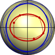
A conic $C$ is said to contain a set $\mathcal{L}$ of straight lines if every member $L\in\mathcal{L}$ has at most one real intersection point with $C$ . In this sense, one may ask for the enclosing conic of minimal size with respect to the measure $m$ (Figure 4). As corollary to Theorem 8 we can state

Corollary 10.

Let $\mathcal{L}\subset S^{2}$ be a set of lines such that its polar set $p(\mathcal{L})$ satisfies the requirements of Theorem 3. Among all conics with two given axes that contain $\mathcal{L}$ there exists exactly one of minimal measure.

Corollary 11.

Let $\mathcal{L}\subset S^{2}$ be a set of lines such that its polar set $p(\mathcal{L})$ satisfies the requirements of Theorem 5. Among all conics with given center that contain $\mathcal{L}$ there exists exactly one of minimal measure.

Corollary 12.

Let $\mathcal{L}\subset S^{2}$ be a compact set of lines that is contained in a circle of radius $\varrho^{-1}>0$ . Assume there exists an enclosing conic of $\mathcal{L}$ whose measure is larger than the measure for the set of lines contained in a conic of semi-axes lengths $\mathrm{R}^{-1}$ and $\varrho^{-1}$ . Then the enclosing conic of minimal measure $m$ to the line set $\mathcal{L}$ is unique.

6. Conclusion

We have proved uniqueness of the enclosing conic of minimal area in the elliptic plane. If the minimizer is sought within a set of conics with prescribed axes or center, it is unique at any rate (Theorem 3 and Theorem 5). In the most general setting we can show uniqueness only under additional assumptions on the enclosed set $F$ (Theorems 8). In particular, $F$ must be contained in a circle of radius $\mathrm{R}$ . Given the fact that the diameter of the elliptic plane is $\pi$ , the bounds on the size of $F$ seem acceptable for many applications. The question whether the conditions on $F$ can be relaxed remains open. Example 6 on Page 6 shows that the method of in-between conics is not capable of proving uniqueness without additional constraints on $F$ .

Open questions in the area of extremal quadrics are numerous. Starting from this article it would be natural to consider uniqueness results for size functions different from the area and uniqueness of maximal inscribed conics, generalizations to higher dimensions and other non-Euclidean geometries, for example the hyperbolic plane.

Appendix A Proofs of auxiliary results

In this appendix we prove technical results which are needed in the proofs of our main theorems but are probably of little interest otherwise.

Lemma 13.

For $C$ as defined in (40) we have $C<0$ .

Proof.

Inserting (36) and (37) into the defining Equation (40) of $C$ we obtain the integral representation

(53)

C=-2\int_{0}^{1}\frac{(\nu_{0,1}-\nu_{0,2})\sqrt{1-t^{2}}\sqrt{\nu_{0,1}(1+\nu_{0,2})}}{\sqrt{t^{2}(\nu_{0,2}-\nu_{0,1})+\nu_{0,1}(1+\nu_{0,2})}}\operatorname{d\!}t

Obviously, the integral is positive so that $C$ is negative. ∎

Lemma 14.

For $A$ as defined in (40) we have $A<C$ .

Proof.

We view $A$ and $C$ as functions of $\nu_{0,1}$ and $\nu_{0,2}$ and show that the inequality $A<C$ holds for every $\nu_{0,1}$ -parameter line. For $\nu_{0,1}=\nu_{0,2}$ (which we generally exclude, see Subsection 4.2.1) we have $\bar{E}=\bar{K}$ . Therefore, the function $D(\nu_{0,1},\nu_{0,2})=A(\nu_{0,1},\nu_{0,2})-C(\nu_{0,1},\nu_{0,2})$ vanishes for $\nu_{0,1}=\nu_{0,2}$ . The same is true for its derivative with respect to $\nu_{0,1}$ which can be computed as

(54)

\mathinner{\dfrac{\partial{}D}{\partial{\nu_{0,1}}}}(\nu_{0,1},\nu_{0,2})=\frac{2\nu_{0,1}(2\nu_{0,1}+\nu_{0,2})(\bar{E}-\bar{K})-(2\nu_{0,1}+\nu_{0,2})\bar{K}+3\nu_{0,1}\bar{E}}{\nu_{0,1}}.

If we can show that $D$ is strictly concave in $\nu_{0,1}$ on $\nu_{0,1}>\nu_{0,2}$ we may also conclude $D<0$ for $\nu_{0,1}>\nu_{0,2}$ . The second partial derivative with respect to $\nu_{0,1}$ reads

(55)

\mathinner{\dfrac{\partial{{}^{2}}D}{\partial{\nu_{0,1}^{2}}}}=\frac{1}{2\nu_{0,1}^{2}(1+\nu_{0,1})}\big{(}(8\nu_{0,1}^{3}+4\nu_{0,1}^{2}-2\nu_{0,1}-\nu_{0,1}\nu_{0,2})\bar{E}\\ -(8\nu_{0,1}^{3}+8\nu_{0,1}^{2}-\nu_{0,1}\nu_{0,2}-\nu_{0,2})\bar{K}\big{)}.

We have to show that it is negative for $\nu_{0,1}>\nu_{0,2}$ . Because of $\bar{E}<\bar{K}$ we have

(56)

(8\nu_{0,1}^{3}+4\nu_{0,1}^{2})(\bar{E}-\bar{K})<0.

By subtracting (56) from (55) we see that

(57)

(-2\nu_{0,1}-\nu_{0,1}\nu_{0,2})\bar{E}-(4\nu_{0,1}^{2}-\nu_{0,1}\nu_{0,2}-\nu_{0,2})\bar{K}<0

is sufficient for the negativity of (55). Moreover, we have $\nu_{0,1}\nu_{0,2}<\nu_{0,1}^{2}$ so that it enough to show

(58)

(-2\nu_{0,1}-\nu_{0,1}\nu_{0,2})\bar{E}-(3\nu_{0,1}^{2}-\nu_{0,2})\bar{K}<0.

Clearly the inequality

(59)

(-\nu_{0,1}-\nu_{0,1}\nu_{0,2})\bar{E}-3\nu_{0,1}^{2}\bar{K}<0

holds true. Subtracting (59) from (58), we arrive at

(60)

\nu_{0,2}\bar{K}-\nu_{0,1}\bar{E}<0.

We write $\nu_{0,2}\bar{K}-\nu_{0,1}\bar{E}$ in its integral form

(61)

\nu_{0,2}\bar{K}-\nu_{0,1}\bar{E}=-\frac{\nu_{0,1}-\nu_{0,2}}{1+\nu_{0,2}}\int_{0}^{1}\frac{1+\nu_{0,2}-t^{2}}{\sqrt{1-t^{2}}\sqrt{1-f^{2}t^{2}}}\operatorname{d\!}t

and observe that the factor before the integral is negative while the denominator of the integrand is positive. Moreover, the numerator of the integrand is linear in $t^{2}$ . For $t=0$ it equals $1+\nu_{0,2}>0$ and for $t=1$ it equals $\nu_{0,2}>0$ . Thus, it is positive for $t\in[0,1]$ . We conclude that (57) holds true. Hence, the $\nu_{0,1}$ -parameter lines of $D$ are strictly concave so that indeed $A<C$ . ∎

Lemma 15.

If $\nu_{0,2}>v_{0}$ (this is implied by the assumptions of Theorem 8) we have $B<A$ .

Proof.

We show that $2A-B-C\geq 0$ . Because of $A-C<0$ this implies $B<A$ . We have

(62)

2A-B-C=6\nu_{0,1}(1+\nu_{0,1})\bar{E}-2(2\nu_{0,1}+\nu_{0,2})(1+\nu_{0,1})\bar{K}.

This expression is not negative if and only if

(63)

3\nu_{0,1}\bar{E}-(2\nu_{0,1}+\nu_{0,2})\bar{K}\geq 0.

Writing $\bar{E}$ and $\bar{K}$ in their integral forms we get

(64)

I\mathrel{\mathop{\ordinarycolon}}=3\nu_{0,1}\bar{E}-(2\nu_{0,1}+\nu_{0,2})\bar{K}=\frac{\nu_{0,1}-\nu_{0,2}}{1+\nu_{0,2}}\int_{0}^{1}\frac{1+\nu_{0,2}-3t^{2}}{\sqrt{1-t^{2}}\sqrt{1-f^{2}t^{2}}}\operatorname{d\!}t

where $f$ is given by (37). We have to show that $I$ is not negative. This is obviously true for $\nu_{0,2}\geq 2$ because then the integrand is positive for $t\in(0,1)$ . But we can do even better. Assume $\nu_{0,2}<2$ and denote by $w=\sqrt{(1+\nu_{0,2})/3}$ the unique root of the integrand. We split the integral (64) into a positive and a negative part $I=I_{1}+I_{2}$ where

(65)

I_{1}=\frac{\nu_{0,1}-\nu_{0,2}}{1+\nu_{0,2}}\int_{0}^{w}\frac{1+\nu_{0,2}-3t^{2}}{\sqrt{1-t^{2}}\sqrt{1-f^{2}t^{2}}}\operatorname{d\!}t

and

(66)

I_{2}=\frac{\nu_{0,1}-\nu_{0,2}}{1+\nu_{0,2}}\int_{w}^{1}\frac{1+\nu_{0,2}-3t^{2}}{\sqrt{1-t^{2}}\sqrt{1-f^{2}t^{2}}}\operatorname{d\!}t.

Since $f^{2}=(\nu_{0,1}-\nu_{0,2})/(\nu_{0,1}(1+\nu_{0,2}))$ is monotone increasing in $\nu_{0,1}$ we have

(67)

0\leq f^{2}\leq\lim_{\nu_{0,1}\to\infty}f^{2}=\frac{1}{1+\nu_{0,2}}.

Using this we find

(68)

1\leq\frac{1}{\sqrt{1-f^{2}t^{2}}}\leq\frac{\sqrt{1+\nu_{0,2}}}{\sqrt{1+\nu_{0,2}-t^{2}}}\qquad\text{for}~t\in[0,1].

Thus, we can estimate

(69)			$\displaystyle I_{1}\geq\frac{\nu_{0,1}-\nu_{0,2}}{1+\nu_{0,2}}\int_{0}^{w}\frac{1+\nu_{0,2}-3t^{2}}{\sqrt{1-t^{2}}}\operatorname{d\!}t\quad\text{and}$
(69)			$\displaystyle I_{2}\geq\frac{\nu_{0,1}-\nu_{0,2}}{1+\nu_{0,2}}\int_{w}^{1}\frac{(1+\nu_{0,2}-3t^{2})\sqrt{1+\nu_{0,2}}}{\sqrt{1-t^{2}}\sqrt{1+\nu_{0,2}-t^{2}}}\operatorname{d\!}t.$

This allows to discuss the non-negativity of

(70)

\int_{0}^{w}\frac{1+\nu_{0,2}-3t^{2}}{\sqrt{1-t^{2}}}\operatorname{d\!}t+\int_{w}^{1}\frac{(1+\nu_{0,2}-3t^{2})\sqrt{1+\nu_{0,2}}}{\sqrt{1-t^{2}}\sqrt{1+\nu_{0,2}-t^{2}}}\operatorname{d\!}t

instead of $I_{1}+I_{2}$ . But this is guaranteed by the Theorem’s assumptions (compare with Equation (24)). ∎

Lemma 16.

Under the assumptions $\nu_{0,2}>v_{0}$ and (41) ( $r_{3}^{2}-r_{1}^{2}\geq 0$ ) we have

(71)

(2B-A-C)r_{3}^{2}+(A-C)(r_{2}^{2}-r_{1}^{2})\leq 0.

Proof.

We write (71) as

(72)

(2B-A-C)r_{3}^{2}+(A-C)(r_{2}^{2}-r_{1}^{2})\\ =(B-A)r_{3}^{2}-(A-C)r_{1}^{2}+(B-C)r_{3}^{2}+(A-C)r_{2}^{2}.

The non-positivity of $(B-A)r_{3}^{2}-(A-C)r_{1}^{2}$ is shown in the proof of Lemma 17 in (75). The Lemma’s claim follows from the fact that the remaining terms are not positive. ∎

Lemma 17.

Under the assumptions $\nu_{0,2}>v_{0}$ and (41) ( $r_{3}^{2}-r_{1}^{2}\geq 0$ ) we have

(73)

r_{1}^{2}r_{2}^{2}(C-A)(\nu_{1,1}-\nu_{1,2})+r_{1}^{2}r_{3}^{2}(B-C)(1+\nu_{1,2})+r_{2}^{2}r_{3}^{2}(B-A)(1+\nu_{1,1})\leq 0.

Proof.

We write (73) as

(74)

\begin{gathered}r_{3}^{2}(r_{1}^{2}(B-C)+r_{2}^{2}(B-A))+r_{1}^{2}(r_{2}^{2}(A-C)+r_{3}^{2}(B-C))\nu_{1,2}\\ +r_{2}^{2}(-r_{1}^{2}(A-C)+r_{3}^{2}(B-A))\nu_{1,1}.\end{gathered}

The first row is not positive; the second row needs closer investigation. We know that $B-A\leq A-C$ because of $2A-B-C\geq 0$ (see the proof of Lemma 15). Therefore we can bound the relevant factor of the second row of (74) according to

(75)

-r_{1}^{2}(A-C)+r_{3}^{2}(B-A)\leq(A-C)(r_{3}^{2}-r_{1}^{2})\leq 0.

This implies that (74) and therefore (73) is not-positive. ∎

Acknowledgments

The authors gratefully acknowledge support of this research by the Austrian Science Foundation FWF under grant P21032 (Uniqueness Results for Extremal Quadrics).

References

Barequet and Elber [2005] G. Barequet and G. Elber. Optimal bounding cones of vectors in three dimensions. Inform. Process. Lett., 93(2):83–89, 2005.
Behrend [1937] F. Behrend. Über einige Affininvarianten konvexer Bereiche. Math. Ann., 113:712–747, 1937.
Behrend [1938] F. Behrend. Über die kleinste umbeschriebene und die größte einbeschriebene Ellipse eines konvexen Bereiches. Math. Ann., 115:397–411, 1938.
Danzer et al. [1957] L. Danzer, D. Laugwitz, and H. Lenz. Über das Löwnersche Ellipsoid und sein Analogon unter den einem Eikörper einbeschriebenen Ellipsoiden. Arch. Math., 8(3):214–219, 1957.
Davis [1957] Ch. Davis. All convex invariant functions of Hermitian matrices. Arch. Math., 8(4):276–278, 1957.
Firey [1964] W. J. Firey. Some applications of means of convex bodies. Pacific J. Math., 14(1):53–60, 1964.
Gruber [2008] P. M. Gruber. Application of an idea of Voronoi to John type problems. Adv. in Math., 218(2):309–351, 2008.
John [1948] F. John. Studies and essays. Courant anniversary volume, chapter Extremum problems with inequalities as subsidary conditions, pages 187–204. Interscience Publ. Inc., New York, 1948.
Juhnke [1990] F. Juhnke. Volumenminimale Ellipsoidüberdeckungen. Beitr. Algebra Geom., 30:143–153, 1990.
Juhnke [1994] F. Juhnke. Embedded maximal ellipsoids and semi-infinite optimization. Beitr. Algebra Geom., 35(2):163–171, 1994.
Klartag [2004] B. Klartag. On John-type ellipsoids. In Geometric Aspects of Functional Analysis, Lecture Notes in Mathematics, pages 149–158. Springer, Berlin, Heidelberg, 2004.
Lawson [1965] C. Lawson. The smallest covering cone or sphere. SIAM Rev., 7(3):415–417, 1965.
Lewis [1996] A. S. Lewis. Convex analysis on the Hermitian matrices. SIAM J. Optim., 6(1):164–177, 1996.
Schröcker [2007] H.-P. Schröcker. Minimal enclosing hyperbolas of line sets. Beitr. Algebra Geom., 48(2):367–381, 2007.
Schröcker [2008] H.-P. Schröcker. Uniqueness results for minimal enclosing ellipsoids. Comput. Aided Geom. Design, 25(9):756–762, 2008.
Weber and Schröcker [2010] M. J. Weber and H.-P. Schröcker. Davis’ convexity theorem and extremal ellipsoids. Beitr. Algebra Geom., 51(1):263–274, 2010.