Minimising quantifier variance under prior probability shift

The survey paper [8] described the problem to estimate prior class probabilities (also called prevalences) on a test set with a different distribution than the training set (the quantification problem) as “Given a labelled training set, induce a quantifier that takes an unlabelled test set as input and returns its best estimate of the class distribution.” As becomes clear from [8] and also more recent work on the problem, it has been widely investigated in the past twenty years.

A lot of different approaches to quantification of prior class probabilities has been proposed and analysed (see, e.g. [8, 10, 16]), but it appears that the following question has not yet received very much attention:

Is it worth the effort to try to train a good (accurate) hard (or soft or probabilistic) classifier as the ‘base classifier’ for the task of quantification if the class labels of individual instances are unimportant and only the aggregate prior class probabilities are of interest?

In principle, there is a clear answer to this question. The accuracy of the classifier matters at least in the extreme cases:

• •

  If a classifier is least accurate because its predictions and the true class labels are stochastically independent, then quantification is not feasible.

• •

  If a classifier is most accurate in the sense of making perfect predictions then perfect quantification is easy by applying Classify & Count [4].

But if no perfect classifier is around, can we be happy to deploy a moderately accurate classifier for quantification or should we rather strive to develop an optimal classifier, possibly based on an comprehensive feature selection process?

Some researchers indeed suggest that the accuracy of the base classifiers is less important for quantification than for classification. [5] made the following statements:

• •

  From the abstract of [5]: “These strengths can make quantification practical for business use, even where classification accuracy is poor.”

• •

  P. 165 of [5]: “The effort to develop special purpose features or classifiers could increase the cost significantly, with no guarantee of an accurate classifier. Thus, an imperfect classifier is often all that is available.”

• •

  P. 166 of [5]: “It is sufficient but not necessary to have a perfect classifier in order to estimate the class distribution well. If the number of false positives balances against false negatives, then the overall count of predicted positives is nonetheless correct. Intuitively, the estimation task is easier for not having to deliver accurate predictions on individual cases.”

The point on the mutual cancellation of false positives and false negatives is mentioned also by a number of other researchers like for instance [3]. On p. 74, [3] wrote: “Equation 1 [with the definition of the $F$-measure] shows that $F_{1}$ deteriorates with $(FP+FN)$ and not with $|FP-FN|$, as would instead be required of a function that truly optimizes quantification.”

There are also researchers that hold the contrary position, at least as quantification under an assumption of prior probability shift (see (3.1) below for the formal definition) is concerned:

• •

  [25] noted for the class of ‘ratio estimators’ they introducted that it was both desirable and feasible to construct estimators with small asymptotic variances.

• •

  [22] demonstrated by a simulation study that estimating the prior class probabilities by means of a more accurate base classifier may entail much shorter confidence intervals for the estimates.

• •

  [1, 7] pointed out the efficiency of the maximum likelihood estimator (MLE) for the quantification task and made cases for its application.

In the following, we revisit the question of the usefulness of accurate classifiers for quantification:

After giving an overview of related research in Section 2 and specifying the setting and assumptions for the binary quantification problem in Section 3, we recall the technical details of the definition of the MLE for the positive class prevalence in Section 4. In particular, we show that the MLE is well-defined under the mild condition that the test sample consists of at least two different points, see (4.4) below.

In Section 5, we describe, based on its representation in terms of the Fisher information, the Cramér-Rao lower bound for the variances of unbiased estimators of the positive class prevalence, see (5.1) below. This lower bound, at the same time, is the large sample variance of the MLE defined in Section 4. Thus, the Cramér-Rao lower bound is achievable in theory by MLEs – which might explain to some extent the superiority of MLEs as observed in [1, 7].

In Section 6, we show for the test distribution of the feature vector that its associated Fisher information with respect to the positive class prevalence is – up to a factor depending only on the true prevalence – just the variance of the posterior positive class probability (Proposition 6.1 below). The variance of the posterior probability is closely related to the Brier score for the regression of the class label on the feature vector. While the Brier score decreases when the information content of the feature vector increases, the variance of the posterior probability decreases with shrinking information content of the features. In any case, these observations imply that the large sample variance of the MLE (or the Cramér-Rao lower bound for the variances of unbiased estimators) may be reduced when a feature vector with larger information content is selected. Section 6 concludes with two suggestions of how this can be achieved in practice (Brier curves, ROC analysis).

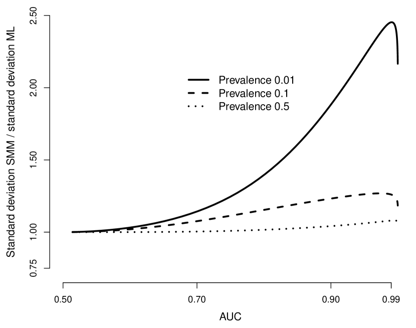
In Section 7, we illustrate the observations of Sections 5 and 6 with a numerical example. Table 1 below demonstrates variance reduction through more powerful features both for the ML quantifier and a non-ML quantifier. Figure 1 below suggests that differences in efficiency between the ML quantifier and non-ML quantifiers may depend both on the information content (power) of the feature vector and on the true value of the positive class prevalence.

Prior probability shift is a special type of data set shift, see [15] for background information and a taxonomy of data set shift. In the literature, also other terms are used for prior probability shift, for instance ‘global drift’ [12] or ‘label shift’ [13].

The problem of estimating the test set prior class probabilities can also be interpreted as a problem to estimate the parameters of a ‘mixture model’ [6] where the component distributions are learnt on a training set. See [17] for an early work on the properties of the maximum likelihood (ML) estimator in this case. [20] revived the interest in the ML estimator for the unknown prior class probabilities in the test set by specifying the associated ‘expectation maximisation’ (EM) algorithm.

[21] proposed to take recourse to the notion of Fisher consistency as a criterion to identify completely unsuitable approaches to the quantification problem that do not have this property. [21] then proved Fisher consistency of the ML estimator under prior probability shift.

The ML approach has been criticised for its sometimes moderate performance and the effort and amount of training data needed to implement it. However, recently some researchers [1, 7] began to vindicate the ML approach. They focussed on the need to properly calibrate the posterior class probability estimate in order to improve the efficiency of the MLE for the positive class prevalence on the test set. Complementing the work of [1, 7], in this paper we study the role that constructing more powerful (or accurate) classifiers by selection of more appropriate features may play to reduce the variances of the related quantifiers.

In the following, we revisit the well-known asymptotic efficiency property of ML estimators in the special case of the MLE for prior class probabilities in the binary setting and investigate how it is impacted by the power (accuracy) of the classifier on the MLE is based.

We consider the binary prevalence quantification problem in the following setting:

• •

  There is a training (or source) data set $(x_{1},y_{1}),\ldots,(x_{m},y_{m})\in\mathfrak{X}\times\{0,1\}$. It is assumed to be an i.i.d. sample of a random vector $(X,Y)$ with values in $\mathfrak{X}\times\{0,1\}$. The vector $(X,Y)$ is defined on a probability space $(\Omega,P)$, the training (or source) domain. The elements $\omega$ of $\Omega$ are the instances (or objects). Each instance $\omega$ belongs to one of the classes $0$ and $1$, and its class label is $Y(\omega)\in\{0,1\}$. In addition, each instance $\omega$ has features $X(\omega)\in\mathfrak{X}$. Often, $\mathfrak{X}$ is the $d$-dimensional Euclidian space such that accordingly $X$ is a real-valued random vector. See Appendix B.1 of [27] for more detailed comments of how this setting avoids the logical problems that arise when feature vectors and instances are considered to be the same thing.

• •

  Under the training distribution $P$, both the features $X(\omega)$ and the class labels $Y(\omega)$ of the instances are observed in a series of $m$ independent experiments resulting in the sample $(x_{1},y_{1}),\ldots,(x_{m},y_{m})$. The sample can be used to infer the joint distribution of $X$ and $Y$ under $P$, and hence, in particular, also the distribution of $Y$ (the class distribution) under $P$.

• •

  There is a test (or target) data set $z_{1},\ldots,z_{n}\in\mathfrak{X}$. It is assumed to be an i.i.d. sample of the random vector $X$ with values in $\mathfrak{X}$, under a probability measure $Q$ on $\Omega$ that may be different to the training distribution $P$.

• •

  Under the test distribution $Q$, only the features $X(\omega)$ of the instances are observed in a series of $n$ independent experiments resulting in the sample $z_{1},\ldots,z_{n}$. The sample can be used to infer the distribution of $X$ under $Q$.

• •

  The goal of quantification is to infer the distribution of $Y$ under $Q$, based on the sample of features $z_{1},\ldots,z_{n}$ generated under $Q$ and on the joint sample of features and class labels $(x_{1},y_{1}),\ldots,(x_{m},y_{m})$ generated under $P$. It is not possible to design a method for this inference without any assumption on the relation of $P$ and $Q$.

• •

  In this paper, we assume that $P$ and $Q$ are related by prior probability shift, in the sense that the class-conditional feature distributions are the same under $P$ and $Q$, i.e. it holds that

  $$P[X\in M\,|\,Y=i]\ =\ Q[X\in M\,|\,Y=i]$$

  (3.1)

  for $i\in\{0,1\}$ and all measurable subsets $M$ of $\mathfrak{X}$.

Denoting $P[Y=1]=p$ and $Q[Y=1]=q$, (3.1) implies that the distribution of the features $X$ under $P$ and $Q$ respectively can be represented as

	$\displaystyle P[X\in M]$	$\displaystyle=p\,P[X\in M\,|\,Y=1]+(1-p)\,P[X\in M\,|\,Y=0],$		(3.2a)
	$\displaystyle Q[X\in M]$	$\displaystyle=q\,P[X\in M\,|\,Y=1]+(1-q)\,P[X\in M\,|\,Y=0],$		(3.2b)

for $M\subset\mathfrak{X}$. In the following, we assume that the components $p$, $P[X\in M\,|\,Y=1]$ and $P[X\in M\,|\,Y=0]$ can be perfectly estimated from the training sample $(x_{1},y_{1}),\ldots,(x_{m},y_{m})$.

Basically, this means letting $m=\infty$ which obviously is infeasible. The assumption helps, however, to shed light on the importance of both maximum likelihood estimation and accurate classifiers for the efficient estimation of the unknown positive class prevalence $q$ in the test data set.

Assume that the conditional distributions in (3.1) have positive densities $f_{i}$, $i=0,1$. Then the unconditional density of the features vector $X$ under $Q$ is

$$f^{(q)}(x)\ =\ (1-q)\,f_{0}(x)+q\,f_{1}(x),\quad x\in\mathfrak{X}.$$

(4.1)

Hence the likelihood function

$$L_{n}(q)=L_{n}(q;z_{1},\ldots,z_{n})$$

for the sample $z_{1},\ldots,z_{n}$ is given by

$$L_{n}(q)\ =\ \prod_{i=1}^{n}\bigl{(}q\,(f_{1}(z_{i})-f_{0}(z_{i}))+f_{0}(z_{i})\bigr{)}.$$

(4.2)

This implies for the first two derivatives of the log-likelihood with respect to $q$:

	$\displaystyle\frac{\partial\log L_{n}}{\partial\,q}(q)$	$\displaystyle=\sum_{i=1}^{n}\frac{f_{1}(z_{i})-f_{0}(z_{i})}{q\,(f_{1}(z_{i})-f_{0}(z_{i}))+f_{0}(z_{i})},$		(4.3a)
	$\displaystyle\frac{\partial^{2}\log L_{n}}{\partial\,q^{2}}(q)$	$\displaystyle=-\sum_{i=1}^{n}\left(\frac{f_{1}(z_{i})-f_{0}(z_{i})}{q\,(f_{1}(z_{i})-f_{0}(z_{i}))+f_{0}(z_{i})}\right)^{2}\leq 0.$		(4.3b)

We assume that there is at least one $j\in\{1,\ldots,n\}$ such that

$$f_{1}(z_{j})\ \neq\ f_{0}(z_{j}).$$

(4.4)

Under (4.4), $q\mapsto\log L_{n}(q)$ is strictly concave in $[0,1]$. Hence (see Example 4.3.1 of [24]) the equation

$$\frac{\partial\log L_{n}}{\partial\,q}(q)\ =\ 0$$

(4.5)

has a solution $0<q<1$ if and only if

	$$\begin{split}\frac{1}{n}\sum_{i=1}^{n}\frac{f_{1}(z_{i})}{f_{0}(z_{i})}>1\quad\text{and}\quad\frac{1}{n}\sum_{i=1}^{n}\frac{f_{0}(z_{i})}{f_{1}(z_{i})}>1.\end{split}$$		(4.6a)
This solution is then the unique point in $[0,1]$ where $L_{n}(q)$ takes its absolute maximum value. By strict concavity of $\log L_{n}$, if (4.6a) is not true then either
	$$\begin{split}\frac{1}{n}\sum_{i=1}^{n}\frac{f_{1}(z_{i})}{f_{0}(z_{i})}\leq 1\quad\text{and}\quad\frac{1}{n}\sum_{i=1}^{n}\frac{f_{0}(z_{i})}{f_{1}(z_{i})}>1,\end{split}$$		(4.6b)
applies or
	$$\begin{split}\frac{1}{n}\sum_{i=1}^{n}\frac{f_{1}(z_{i})}{f_{0}(z_{i})}>1\quad\text{and}\quad\frac{1}{n}\sum_{i=1}^{n}\frac{f_{0}(z_{i})}{f_{1}(z_{i})}\leq 1,\end{split}$$		(4.6c)
holds. Under (4.6b), the unique maximum of $\log L_{n}$ in $[0,1]$ lies at $q=0$ while under (4.6c), the unique maximum of $\log L_{n}$ in $[0,1]$ is taken at $q=1$.

In summary, under the natural assumption (4.4), the likelihood function $L_{n}$ of (4.2) has an absolute maximum in $[0,1]$ at a unique point $q^{\ast}\in[0,1]$. As a consequence, the maximum likelihood (ML) estimate $\hat{q}_{n}$ of the test set positive class prevalence $q$ is well-defined by setting $\hat{q}_{n}=q^{\ast}$.

In the setting of Section 3, let $\widetilde{q}_{n}$ be any unbiased estimator of the positive class prevalence $q$ under the test distribution $Q$, i.e. $\widetilde{q}_{n}=W_{n}(X_{1},\ldots,X_{n})$ for some function $W_{n}:\mathfrak{X}^{n}\to\mathbb{R}$ such that

$$E_{Q}[\widetilde{q}_{n}]=Q[Y=1]=q,$$

where $E_{Q}$ denotes the expected value under the mixture probability measure $Q$ of (3.2b). Assume additionally that there are positive densities $f_{0}$ and $f_{1}$ of the class-conditional distributions of the feature vector $X$, such that the density $f^{(q)}$ of $X$ under $Q$ is given by (4.1).

If $(X_{1},\ldots,X_{n})$ is an i.i.d. sample from the distribution of the feature vector under the test distribution $Q$, then the variance of $\widetilde{q}_{n}$ is bounded from below by the inverse of the product of the Fisher information of the test distribution with respect to $q$ and the size of the sample (Cramér-Rao bound, see, e.g., Corollary 7.3.10 of [2]):

	$\displaystyle\mathrm{var}[\widetilde{q}_{n}]$	$\displaystyle\ \geq\ \frac{1}{n\,E_{Q}\left[\left(\frac{\partial\log f^{(q)}}{\partial\,q}(X)\right)^{2}\right]}$
		$\displaystyle\ =\ \frac{1}{n\,E_{Q}\left[\left(\frac{f_{1}(X)-f_{0}(X)}{f^{(q)}(X)}\right)^{2}\right]}.$		(5.1)

Actually, since $\hat{q}_{n}$ from Section 4 is the ML estimator of $q$, (3.2b) presents not only a lower bound for the variances of unbiased estimators of $q$ but also the large sample variance of $\hat{q}_{n}$ in the sense that $\sqrt{n}\,(\hat{q}_{n}-q)$ converges in distribution toward $\mathcal{N}\left(0,E_{Q}\left[\Big{(}\frac{f_{1}(X)-f_{0}(X)}{f^{(q)}(X)}\Big{)}^{2}\right]^{-1}\right)$, the normal distribution with mean $0$ and variance $E_{Q}\left[\Big{(}\frac{f_{1}(X)-f_{0}(X)}{f^{(q)}(X)}\Big{)}^{2}\right]^{-1}$, the asymptotic variance of $\hat{q}_{n}$ (see, e.g., Theorem 10.1.12 of [2]). Note that the lower bound of (5.1) may not hold for $\hat{q}_{n}$ because it need not be unbiased.

In summary, if the densities of the class-conditional feature distributions are known, the ML estimator of $q$ has asymptotically the smallest variance of all unbiased estimators of $q$ on i.i.d. samples from the test distribution of the features. This is demonstrated in the two upper panels of Table 4 of [22] which shows on simulated data that confidence intervals for $q$ – which are primarily driven by the standard deviations of the estimators – based on the ML estimator are the shortest if the training sample is infinite and the test sample is large.

From Proposition 6.1 we obtain the following representation of the asymptotic variance of the ML estimator $\hat{q}_{n}$:

$$E_{Q}\left[\Big{(}\frac{f_{1}(X)-f_{0}(X)}{f^{(q)}(X)}\Big{)}^{2}\right]^{-1}=\frac{q^{2}\,(1-q)^{2}}{\mathrm{var}_{Q}[\eta_{Q}(X)]}.$$

(6.2)

Recall the following decomposition of the optimal Brier Score $BS_{Q}(X)$ for the problem to predict the class variable $Y$ from the features $X$ (under the test distribution $Q$):

	$\displaystyle BS_{Q}(X)$	$\displaystyle\ =\ E_{Q}\left[(Y-\eta_{Q}(x))^{2}\right]$
		$\displaystyle\ =\ \mathrm{var}_{Q}[Y]-\mathrm{var}_{Q}[\eta_{Q}(X)]$
		$\displaystyle\ =\ q\,(1-q)-\mathrm{var}_{Q}[\eta_{Q}(X)].$		(6.3)

In (6.3), the optimal Brier Score $BS_{Q}(X)$ is also called refinement loss, while $\mathrm{var}_{Q}[Y]$ and $\mathrm{var}_{Q}[\eta_{Q}(X)]$ are known as uncertainty and resolution respectively [9].

By (6.2), the asymptotic variance of the ML estimator $\hat{q}_{n}$ is reduced if a feature vector $X$ with greater variance of $\eta_{Q}(X)$ is found (or if the Brier Score with respect to $X$ decreases). Consider, for instance, a feature vector $X^{\prime}$ that is a function of the feature vector $X$, i.e. it holds that $X^{\prime}=F(X)$ for some function $F:\mathfrak{X}\to\mathfrak{X}^{\prime}$. Since $F$ potentially maps different values $x\in\mathfrak{X}$ onto the same value $x^{\prime}\in\mathfrak{X}^{\prime}$ the amount of information carried by $X^{\prime}$ is reduced compared to the amount of information carried by $X$. Therefore, the approximation of the class label $Y$ by regression on $X^{\prime}$ is less close than the approximation of $Y$ by regression on $X$.

From this observation, it follows that $BS_{Q}(X^{\prime})\geq BS_{Q}(X)$. This in turn implies by (6.3) and (6.2) for the asymptotic variances of the ML estimators $\hat{q}_{n}(X^{\prime})$ and $\hat{q}_{n}(X)$ that

$$\mathrm{var}_{Q}[\hat{q}_{n}(X^{\prime})]\ \leq\ \mathrm{var}_{Q}[\hat{q}_{n}(X)].$$

(6.4)

Observe that $X^{\prime}=F(X)$ also implies $BS_{P}(X^{\prime})\geq BS_{P}(X)$, i.e. also under the training distribution $P$, the posterior positive class probability $\eta_{P}(X)$ based on $X$ is a better predictor of $Y$ than $\eta_{P}(X^{\prime})$ which is based on $X^{\prime}$. By the assumption underlying this paper, $BS_{P}(X^{\prime})$ and $BS_{P}(X)$ are observable while $BS_{Q}(X^{\prime})$ and $BS_{Q}(X)$ are not, because the class label $Y$ is not observed in the test data set.

But does $BS_{P}(X^{\prime})\geq BS_{P}(X)$ always imply $BS_{Q}(X^{\prime})\geq BS_{Q}(X)$ and therefore also (6.4), thus generalising the implication “$X^{\prime}=F(X)$ $\Rightarrow$ (6.4)”?

This paper has no fully general answer to this question. Instead we can only point to alternative conditions on $X^{\prime}$ and $X$ that imply both $BS_{P}(X^{\prime})\geq BS_{P}(X)$ and $BS_{Q}(X^{\prime})\geq BS_{Q}(X)$, but are weaker than $X^{\prime}=F(X)$.

Brier curves:

Recall the notion of Brier curve from [11] (with the slightly modified definition of [23]). If the Brier curve for $\eta_{P}(X^{\prime})$ dominates the Brier curve for $\eta_{P}(X)$, then by item 6) of Proposition 5.2 and Proposition 4.1 of [23], it follows that $BS_{P}(X^{\prime})\geq BS_{P}(X)$ and $BS_{Q}(X^{\prime})\geq BS_{Q}(X)$ hold.

ROC analysis:

Recall the notion of Receiver Operating Characteristic (ROC) as defined, for instance, in [19]. If the ROC for the density ratio associated with $X$ dominates the ROC for the density ratio associated with $X^{\prime}$, then by Remark 5.4 and Proposition 4.1 of [23], it follows that $BS_{P}(X^{\prime})\geq BS_{P}(X)$ and $BS_{Q}(X^{\prime})\geq BS_{Q}(X)$ hold.

In this section, we numerically compare the variance of the Sample Mean Matching (SMM) estimator $\hat{q}_{n,SMM}$ of class prevalences [10] and the Cramér-Rao bound of (5.1) (which is also the large sample variance of the ML estimator $\hat{q}_{n,ML}$ as specified in Section 4 above). In order to be able to do this, we take recourse to the univariate binormal model with equal variances of the class-conditional distributions: The two normal class-conditional distributions of the feature variable $X$ are given by

	$$X\,|\,Y=i\ \sim\ \mathcal{N}(\mu_{i},\sigma^{2}),\qquad i=0,1,$$		(7.1a)
for conditional means $\mu_{0}<\mu_{1}$ and some $\sigma>0$. For the sake of simplicity, we choose
	$$\mu_{0}=0,\quad\mu_{1}>0,\quad\sigma=1.$$		(7.1b)

Greater values of $\mu_{1}$ imply less overlap of the class-conditional feature distributions, corresponding to more powerful (or accurate) models. Or in other words, for greater values of $\mu_{1}$, the feature variable $X$ carries more information on the class label $Y$.

As stated in Section 3, we assume we are dealing with an infinitely large training sample and a test sample of size $n$. By Section 6, then for large $n$ the variance of $\hat{q}_{n,ML}$ is approximately

$$\frac{1}{n}\,E_{Q}\left[\left(\frac{f_{1}(X)-f_{0}(X)}{f^{(q)}(X)}\right)^{2}\right]^{-1},$$

(7.2)

where $Q$ denotes the distribution underlying the test sample and $f_{0}$ and $f_{1}$ are the class-conditional feature densities – which are given for the purpose of this section by (7.1a). We evaluate the term given by (7.2) by means of one-dimensional numerical integration, making use of the R-function ‘integrate’ [18].

From (7.5) und (7.4), it is clear that for fixed test sample size $n$ the variance of $\hat{q}_{n,SMM}$ decreases when the power of the model increases. This is less obvious from (7.2) for the asymptotic variance of $\hat{q}_{n,ML}$ but if follows from (6.2) in that case.

Table 1 above illustrates these observations. In the table, we use the notation

$$\sigma_{SMM}=\sqrt{\mathrm{var}_{Q}[\hat{q}_{n,SMM}]}$$

and

$$\sigma_{ML}=\sqrt{\mathrm{var}_{Q}[\hat{q}_{n,ML}]}.$$

Table 1 suggests the following observations:

• •

  At low levels of model power, small increases of power entail huge reductions of both the SMM variance and the ML large sample variance.

• •

  The variance reductions become moderate or even low for moderate and high levels of model power (higher than 75% AUC).

• •

  The efficiency deficiency of the SMM estimator (as expressed by its variance) compared to the large sample ML variance varies and is much larger for higher levels of model power.

Figure 1 below shows that the efficiency gain of the ML estimator compared to the SMM estimator – assuming an infinitely large training sample – does not only depend on the model power but also on the positive class prevalence.

In this paper, we have revisited the binary quantification problem, i.e. the problem of estimating a binary prior class distribution on the test data set when training and test distributions are different.

• •

  Specifically, under the assumption of prior probability shift we have looked at the asymptotic variance of the maximum likelihood estimator (MLE).

• •

  We have found that this asymptotic variance is closely related to the Brier score for the regression of the class label variable $Y$ against the features vector $X$ under the test set distribution. In particular, the asymptotic variance can be reduced by selection of a more powerful feature vector.

• •

  At the end of Section 6, we have pointed out sufficient conditions and associated training criteria (Brier curves and ROC analysis) for minimising both the Brier score on the training data set and the Brier score on the test data set.

• •

  These findings suggest methods to reduce the variance of the ML estimator of the prior class probabilities (or prevalences) on the test data set. Due to the statistical consistency of ML estimators, by reducing the variance of the estimator also its mean squared error is minimised.

• •

  The large sample variance of the MLE associated with its asymptotic variance is identical to the Cramér-Rao lower bound for the variances of unbiased estimators of the prior positive class probability. Therefore, it seems likely that also other estimators benefit from improved performance of the underlying classifiers or feature vectors.

Indeed, results of a simulation study in [22] and theoretical findings in [25, 26] suggest that improving the accuracy of the base classifiers used for quantification helps to reduce not only the variances of ML estimators but also of other estimators. The example of the Sample Mean Match (SMM) estimator we have discussed in Section 7 supports this conclusion.

However, these findings must be qualified in so far as the observations made in this paper apply only to the case where both training data set and test data set are large. This is a severe restriction indeed as [5] pointed out the importance of quantification methods specifically in the case of small training data sets, for cost efficiency reasons.

Further research on developing efficient quantifiers for small or moderate training and test data set sizes therefore is highly desirable. A promising step in this direction has already been done by [14], with a proposal for the selection of the most suitable quantifiers for problems on data sets with widely varying sizes.

References

- [1] A. Alexandari, A. Kundaje, and A. Shrikumar. Maximum Likelihood with Bias-Corrected Calibration is Hard-To-Beat at Label Shift Adaptation. In International Conference on Machine Learning, pages 222–232. PMLR, 2020.
- [2] G. Casella and R.L. Berger. Statistical Inference. Duxbury Press, second edition, 2002.
- [3] A. Esuli, F. Sebastiani, and A. Abbasi. Sentiment quantification. IEEE intelligent systems, 25(4):72–79, 2010.
- [4] G. Forman. Counting Positives Accurately Despite Inaccurate Classification. In European Conference on Machine Learning (ECML 2005), pages 564–575. Springer, 2005.
- [5] G. Forman. Quantifying counts and costs via classification. Data Mining and Knowledge Discovery, 17(2):164–206, 2008.
- [6] S. Frühwirth-Schnatter. Finite Mixture and Markov Switching Models: Modeling and Applications to Random Processes. Springer, 2006.
- [7] S. Garg, Y. Wu, S. Balakrishnan, and Z. Lipton. A Unified View of Label Shift Estimation. In H. Larochelle, M. Ranzato, R. Hadsell, M. F. Balcan, and H. Lin, editors, Advances in Neural Information Processing Systems, volume 33, pages 3290–3300. Curran Associates, Inc., 2020.
- [8] P. González, A. Castaño, N.V. Chawla, and J.J. Del Coz. A Review on Quantification Learning. ACM Comput. Surv., 50(5):74:1–74:40, 2017.
- [9] D.J. Hand. Construction and Assessment of Classification Rules. John Wiley & Sons, Chichester, 1997.
- [10] W. Hassan, A. Maletzke, and G. Batista. Accurately Quantifying a Billion Instances per Second. In 2020 IEEE 7th International Conference on Data Science and Advanced Analytics (DSAA), pages 1–10, 2020.
- [11] J. Hernández-Orallo, P. Flach, and C. Ferri. Brier Curves: A New Cost-Based Visualisation of Classifier Performance. In Proceedings of the 28th International Conference on Machine Learning (ICML 2011), pages 585–592. International Machine Learning Society, 2011.
- [12] V. Hofer and G. Krempl. Drift mining in data: A framework for addressing drift in classification. Computational Statistics & Data Analysis, 57(1):377–391, 2013.
- [13] Z. Lipton, Y.-X. Wang, and A. Smola. Detecting and Correcting for Label Shift with Black Box Predictors. In J. Dy and A. Krause, editors, Proceedings of the 35th International Conference on Machine Learning, volume 80 of Proceedings of Machine Learning Research, pages 3122–3130. PMLR, 10–15 Jul 2018.
- [14] A.G. Maletzke, W. Hassan, D.M. dos Reis, and G. Batista. The Importance of the Test Set Size in Quantification Assessment. In Proceedings of the Twenty-Ninth International Joint Conference on Artificial Intelligence (IJCAI-20), pages 2640–2646, 2020.
- [15] J.G. Moreno-Torres, T. Raeder, R. Alaiz-Rodriguez, N.V. Chawla, and F. Herrera. A unifying view on dataset shift in classification. Pattern Recognition, 45(1):521–530, 2012.
- [16] A. Moreo, A. Esuli, and F. Sebastiani. QuaPy: A Python-Based Framework for Quantification. arXiv preprint arXiv:2106.11057, 2021.
- [17] C. Peters and W.A. Coberly. The numerical evaluation of the maximum-likelihood estimate of mixture proportions. Communications in Statistics – Theory and Methods, 5(12):1127–1135, 1976.
- [18] R Core Team. R: A Language and Environment for Statistical Computing. R Foundation for Statistical Computing, Vienna, Austria, 2019.
- [19] M. Reid and R.C. Williamson. Information, Divergence and Risk for Binary Experiments. Journal of Machine Learning Research, 12:731–817, 2011.
- [20] M. Saerens, P. Latinne, and C. Decaestecker. Adjusting the Outputs of a Classifier to New a Priori Probabilities: A Simple Procedure. Neural Computation, 14(1):21–41, 2001.
- [21] D. Tasche. Fisher Consistency for Prior Probability Shift. Journal of Machine Learning Research, 18(95):1–32, 2017.
- [22] D. Tasche. Confidence intervals for class prevalences under prior probability shift. Machine Learning and Knowledge Extraction, 1(3):805–831, 2019.
- [23] D. Tasche. Calibrating sufficiently. arXiv preprint arXiv:2105.07283, 2021.
- [24] D.M Titterington, A.F.M. Smith, and U.E. Makov. Statistical analysis of finite mixture distributions. Wiley New York, 1985.
- [25] A. Vaz, R. Izbicki, and R.B. Stern. Prior Shift Using the Ratio Estimator. In Adriano Polpo, Julio Stern, Francisco Louzada, Rafael Izbicki, and Hellinton Takada, editors, International Workshop on Bayesian Inference and Maximum Entropy Methods in Science and Engineering, pages 25–35. Springer, 2017.
- [26] A. Vaz, R. Izbicki, and R.B. Stern. Quantification Under Prior Probability Shift: the Ratio Estimator and its Extensions. Journal of Machine Learning Research, 20(79):1–33, 2019.
- [27] M.-J. Zhao, N. Edakunni, A. Pocock, and G. Brown. Beyond Fano’s Inequality: Bounds on the Optimal F-Score, BER, and Cost-Sensitive Risk and Their Implications. The Journal of Machine Learning Research, 14(1):1033–1090, 2013.