Minimizing back-action through entangled measurements
Abstract
When an observable is measured on an evolving coherent quantum system twice, the first measurement generally alters the statistics of the second one, which is known as measurement back-action. We introduce, and push to its theoretical and experimental limits, a novel method of back-action evasion, whereby entangled collective measurements are performed on several copies of the system. This method is inspired by a similar idea designed for the problem of measuring quantum work [Perarnau-Llobet et al., Phys. Rev. Lett. 118, 070601 (2017)]. By utilizing entanglement as a resource, we show that the back-action can be extremely suppressed compared to all previous schemes. Importantly, the back-action can be eliminated in highly coherent processes.
Introduction—The enthusiasm for probing and describing microscopic systems in the quantum domain motivates the search for ways to measure quantum processes, akin to standard measurements of operators. This task is notoriously challenging due to the fragility of quantum superpositions and invasiveness of measurements, epitomized in the quantum back-action (QBA) effect Braginskii and Vorontsov (1975); Caves et al. (1980); Braginsky and Khalili (1996); Wiseman and Milburn (2010). Given two measurements separated by a certain time interval, there is QBA when the statistics of the second measurement are altered by the presence of the first measurement. It is mostly considered an unpleasant hindrance in experiments, and significant effort has been invested to design back-action-evading (a.k.a. quantum non-demolition) measurements Braginskii and Vorontsov (1975); Caves et al. (1980); Wiseman (1995); Braginsky and Khalili (1996); Kippenberg and Vahala (2008); Wiseman and Milburn (2010); Erhart et al. (2012); Hacohen-Gourgy et al. (2016); Møller et al. (2017); Kono et al. (2018); Pezzè et al. (2018); Wu et al. (2019); Boulebnane et al. . Besides its fundamental interest, QBA also has important consequences for the definition of heat and work fluctuations in quantum thermodynamics Allahverdyan (2014); Solinas and Gasparinetti (2015); Talkner and Hänggi (2016); Bäumer et al. (2018); Levy and Lostaglio and quantum transport Hovhannisyan and Imparato (2019).
In its essence, QBA is an instance of the uncertainty principle Peres (1993). Say, after measuring an observable , the system’s state, , undergoes a unitary evolution , generated by its internal Hamiltonian. Then, an observable is measured. Viewing in the Heisenberg picture, we thus have two operators, and , simultaneously measured on the state , and when , these measurements are incompatible, both in the sense of the uncertainty relations à la Heisenberg Heisenberg (1927); Białynicki-Birula and Mycielski (1975); Peres (1993); Maccone and Pati (2014) and error-disturbance relations à la Arthurs-Kelly Arthurs and Kelly (1965); Ishikawa (1991); Peres (1993); Ozawa (2003); Allahverdyan et al. (2013); Branciard (2013); Erhart et al. (2012); Busch et al. (2014); Buscemi et al. (2014); Perarnau-Llobet and Nieuwenhuizen (2017). Measurement incompatibility can also be described by constructing joint (quasi)probability distributions, with the condition that the marginal distributions be given by the Born rule Wigner (1932); Terletsky (1937); Margenau and Hill (1961); Mückenheim et al. (1986); Nazarov and Kindermann (2003); Hofer (2017). Quasiprobability distributions, generically arising in (sequential) weak measurement scenarios Mitchison et al. (2007); Avella et al. (2017); Kim et al. (2018); Shojaee et al. (2018); Hovhannisyan and Imparato (2019); Pfender et al. (2019); Cujia et al. (2019); Monroe et al. , necessarily feature negative probabilities Margenau and Hill (1961); Cahill and Glauber (1969); Busch (1985); Uffink (1994); Hartle (2004); Allahverdyan (2014); Potts (2019) (which is related to contextuality Spekkens (2008); Pusey (2014); Lostaglio (2018)); joint distributions that do not feature negative probabilities require going beyond the axiomatics of standard “precise” probability theory Allahverdyan and Danageozian (2018).
In this work, we will take a novel approach towards reducing QBA, by using collective measurements on multiple copies of the system of interest. The logic of our approach is as follows. When , the first measurement does not disturb the state, therefore, the second measurement is not affected by it. That is, there is no QBA when the state is, in a sense, classical, and the joint probability is , where and are the eigenprojectors of and , respectively (, ). This statistics coincides with that of the measure-evolve-measure protocol, widely used and discussed in quantum transport Shelankov and Rammer (2003); Nazarov and Kindermann (2003); Esposito et al. (2009); Hovhannisyan and Imparato (2019) and thermodynamics Jarzynski and Wójcik (2004); Talkner et al. (2007); Esposito et al. (2009); Perarnau-Llobet et al. (2017); Levy and Lostaglio .
When , the standard measure-evolve-measure protocol has QBA, and we wish to find new measurement schemes to reduce it (while agreeing with it for ). However, it was recently shown that there cannot exist a state-independent generalized quantum measurement—a positive operator-valued measure (POVM)—that describes the joint statistics of and and coincides with when commutes with Perarnau-Llobet et al. (2017). Hence, our idea is to consider schemes that are allowed to depend on the state, but do so as weakly as possible. To that end, we use measurements that can be realized as state-independent POVMs on several copies of the system 111Only when viewed from the perspective of a single system, these depend on the state. This is motivated by a QBA-reduction technique proposed and implemented in Refs. Perarnau-Llobet et al. (2017); Wu et al. (2019), for the problem of measuring quantum-mechanical work. There, it was also proven that the QBA cannot be removed no matter how many copies one takes; however, significant reduction can be observed even with two copies. Interestingly, the QBA reduction in Refs. Perarnau-Llobet et al. (2017); Wu et al. (2019) was achieved by using factorized measurements (i.e., the POVM elements are in the form of a Kronecker product).
Here, focusing on the two-copy scenario, we go beyond these results and take this scheme to its extreme. By using entangled POVMs, we show that one can reduce the QBA even further, eliminating it completely in an extended parameter range. These enhancements are only possible due to the entangled nature of the measurements, as we also prove in Ref. 222See Supplemental Material at URL, which contains the mathematical details of the theoretical results and technical details of the experimental setup, and further references Virmani and Plenio (2003); Sanpera et al. (1998); Verstraete et al. (2001) that the proposal of Refs. Perarnau-Llobet et al. (2017); Wu et al. (2019) is the optimal not only among factorized POVMs, but among all separable, i.e., possibly correlated but non-entangled, POVMs. We measure the QBA by comparing the statistics of when is performed with that when is not performed. We determine the ultimate QBA-evading measurement on two copies, which turns out to be entangled. Somewhat counterintuitively, zero QBA can be achieved in a class of continuously parameterized highly coherent processes. We experimentally implement a class of such protocols in the discrete photonics regime, for observing minimal QBA in different quantum processes. Our results show the capability of achieving minimal QBA in our photonic setup with considerably low experimental imperfections, and demonstrate the significant advantage gained over non-entangled measurements.
Theoretical framework and results—Let us formalize the discussion above. The statistics of ’s measurement is given by probabilities and, if is not performed, the statistics of is given by . The desired goal is to find a , where constitute a POVM 333Namely, are non-negative Hermitian operators such that Wiseman and Milburn (2010), such that and , for any state . Had such state-independent POVM exist, we would say that and are jointly measurable Busch (1985); Uffink (1994). However, it is well-known that no such state-independent POVM exists that satisfies this goal for general ’s when Busch (1985); Uffink (1994); Ozawa (2003); Branciard (2013). We deal with this impossibility in the following manner. First, we notice that, when ,
| (1) |
where , describes a valid joint statistics and represents two projective measurements (hence the label “TPM”) of and , performed one after another. Then, we recall that state-independent POVMs, that produce whenever , essentially coincide with Perarnau-Llobet et al. (2017), meaning that there is no room for tweaking the QBA.
Therefore, inspired by an approach developed in the context of quantum thermodynamics Perarnau-Llobet et al. (2017); Wu et al. (2019), we extend the class of POVMs by considering state-independent measurements on two copies of the system: we take a general POVM, ( and ),
| (2) |
and require it to satisfy the condition
| (3) |
in other words, to reproduce for any incoherent . Furthermore, since this measurement is intended to describe the QBA effect, we also require the statistics produced by for the first event (measurement of ) to coincide with , for any ; i.e., also satisfies
| (4) |
Lastly, noticing that the set has more than one element (as opposed to single-copy state-independent measurements, for which the above two requirements necessitate the measurement to coincide with ), we fulfill our main goal by finding , with being the magnitude of the QBA itself:
| (5) |
where is the actual statistics of the second measurement. Put differently, we are looking for the POVM that delivers the correct statistics for classical states, always yields the Born rule for the first measurement, and minimizes the QBA for the second measurement (see also the discussion in Ref. Note (2)). Here, we quantified the QBA by the Euclidean distance between the probability distribution of the second measurement as produced by the joint POVM, , and the probability distribution of the second measurement had the first measurement not taken place, . In principle, one could choose other distance measures in (5), but for our problem of interest—a two-level system—all of them will depend only on the ground-state probability and hence yield the same .
For simplicity, we will concentrate on qubits and consider the case of . Moreover, in the single-qubit Hilbert spaces, we will work in the eigenbasis of , , and, since constant shifts, and multiplication by constants, of do not affect the phenomena at hand, w.l.o.g, we can choose . Below, we will sketch how is calculated in this case, and refer the reader to Ref. Note (2) for full details.
We start by considering requirement . With our choice of operators, the TPM POVM elements will be , resulting in
| (6) |
where are or and describes the probability to start in the state and the transition probability from to . Now, taking into account that all four matrices do not depend on the state, Eq. (8) fixes all diagonal elements of these matrices up to some constants and (see Note (2) for the explicit construction). In particular, one diagonal element will always be zero, so the matrices are at most of rank three.
In order to minimize the QBA, we have to divide the construction and analysis into two cases. First, highly coherent unitary operators, that is, evolutions that produce a lot of coherence given a classical state: . Second, slightly coherent unitary operations: . Interestingly, for the first case one can construct a POVM with zero QBA, while it cannot be reduced to zero for the second case.
In the case of highly coherent unitaries, we can write the optimal POVM as four rank-two matrices that are each a convex combination of and a non-trivial pure entangled state. Note that this POVM also satisfies requirement , i.e., . In the case of slightly coherent unitaries, the optimal POVM contains two rank-three matrices and two rank-one matrices. In this case, there is always some back-action proportional to the initial coherence (see Ref. Note (2)).
In both cases, the optimal POVM are entangled, and one may wonder to which extent such quantum correlations are needed. We also show that the separable collective measurement previously proposed in Refs. Perarnau-Llobet et al. (2017); Wu et al. (2019) is in fact the optimal non-entangled POVM. Hence, any advantage reported in this work is possible due to the entangled nature of the measurement (see Ref. Note (2) for details).
Experiment—We now experimentally implement the minimally invasive entangled POVMs derived above.
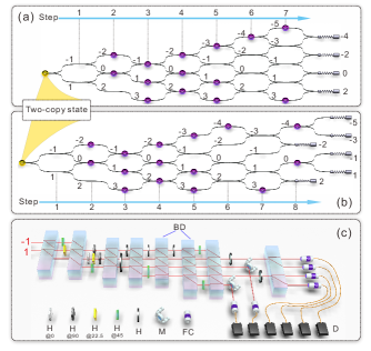
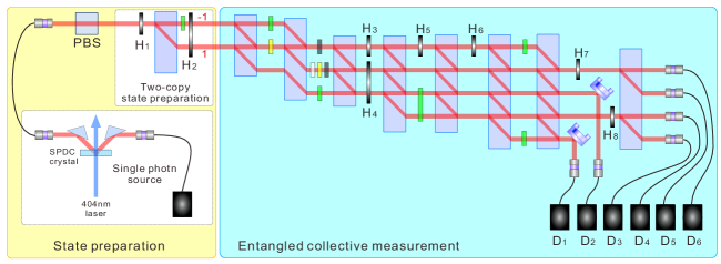
Fig. 1 details both the conceptual design of our quantum walk and the corresponding experimental setup. For state preparation, we make use of multiple degrees of freedom of a down-converted single photon Takeuchi (2001) (spatial mode and polarization). Specifically, we encode the first copy in the spatial degree of freedom, and the second copy in the polarization degree of freedom Wu et al. (2019); Hou et al. (2018), preparing the state , where (see Ref. Note (2) for details).
Experimentally demonstrating the highly non-trivial entangled collective measurements is much more challenging than the separable measurements previously reported in Ref. Wu et al. (2019). The realization of the POVMs can be embedded in the dynamics of a one-dimensional discrete quantum walk Xiao et al. (2017); Hou et al. (2018); Xue et al. (2015); Zhao et al. (2015) containing two degrees of freedom: the walker position, , and a coin state, . The coin qubit and the walker in positions, respectively, and are taken as the two-qubit system of interest, while the other positions of the walker are regarded as an auxiliary system. By engineering the coin operators followed by measuring the walker position after certain steps, a POVM can be deterministically realized with desired outcome at each position. In Figs. 1(a) and (b), the diagram of quantum walks for two cases are shown. The perfect QBA elimination in the case of highly coherent processes can be realized via a step quantum walk, while the slightly coherent case needs steps.
Our all-optical setup is capable of realizing the POVMs for both cases described above. Fig. 1(c) shows the experimental setup for realizing these POVMs. The whole setup is based on a single-photon interferometer. Robust interference between photons in different modes is required to ensure the high-fidelity-implementation of the measurement operators. Details are given in Ref. Note (2).
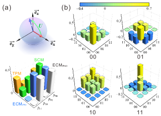
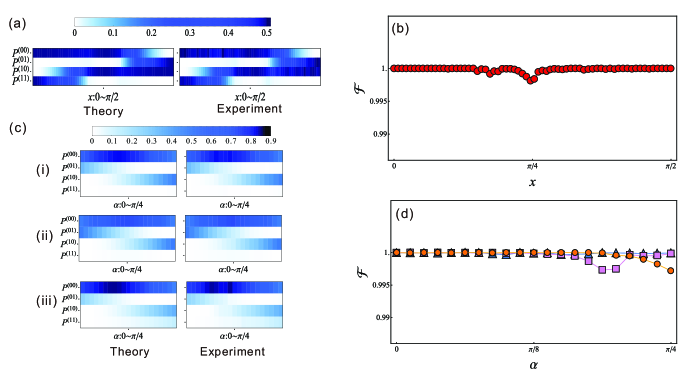
A big entanglement-induced advantage over previous schemes (TPM and the optimal separable collective measurement Perarnau-Llobet et al. (2017)) emerges when . In particular, Fig. 2(a) shows an initial state (red) and final state (blue) in Bloch representation: a pure state is initialized and evolves into , where . The experimentally obtained (where the above a quantity means that is evaluated experimentally) from entangled measurement are presented in Fig. 2(a) as white cubes, while the ideal values given by Eq. (2) are plotted as blue cubes. The expected results obtained from previous schemes are also shown as green (for separable collective measurement) and orange (for TPM) cubes. Fig. 2(b) shows the experimentally reconstructed POVMs, with an average fidelity up to . The fidelity between two POVMs can be defined as , where , and is the fidelity between and Hou et al. (2018).
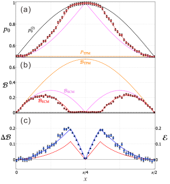
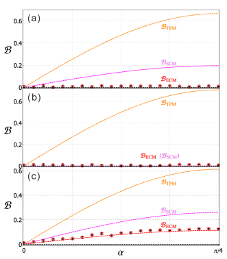
Fig. 3 shows the experimental reduction of QBA for a family of unitaries parameterized as and , where determines the “degree of coherence” of . Fig. 4 shows a similar analysis for different input states and a fixed process. In both figures, the QBA is quantified through Eq. (5).
To observe the divergence between these methods, we first fix the initial state to be the maximally coherent state and implement entangled POVMs so that both highly coherent and slightly coherent processes are included. The results are shown in Fig. 3: (a) shows the probabilities of ending states under various protocols, the experimental values for new entangled POVMs are shown as red disks; (b) shows the experimentally observed QBA for the new POVMs and the simulated values for QBA of previous schemes. The new entangled POVMs (red points) can, within tolerable experimental imperfection, produce probabilities for final states that are closest to the ideal case (black lines), resulting in a significant decrease in QBA compared to the separable measurement. Fig. 3(c) illustrates the fact that any advantage reported in this work is possible due to the entangled nature of the measurement, by showing a comparison between the maximal gain in QBA reduction entangled measurements offer over separable ones and the value of entanglement, as measured by the negativity Horodecki et al. (2009), of the measurement delivering that gain.
We also experimentally test the performance of the new scheme on different inputs (parameterized by ) with fixed . Specifically, we choose , and the coherence of inputs, quantified as , varies from to . The experimentally observed QBA for the entangled POVMs, and the simulated values for all schemes, are shown in Fig. 4, where we can see that the experimentally observed QBA is almost zero for two highly coherent processes and is significantly advantageous over the separable ones for slightly coherent process. The error bars in all figures are estimated by Monte Carlo simulations Note (2).
Conclusions—In this work, we demonstrated that harnessing non-trivial entangled measurements can significantly minimize the QBA. We devised the optimal measurement for reducing the QBA given two copies of a qubit, which turns out to be an entangled measurement. We also proved that the optimal non-entangled measurement coincides with the previous proposal of Perarnau-Llobet et al. (2017); Wu et al. (2019). More specifically, we show that for highly coherent unitary operations the QBA can, in principle, be eliminated. While such an elimination is impossible for slightly coherent unitaries, our new scheme offers a considerable advantage over those using only separable measurements Perarnau-Llobet et al. (2017); Wu et al. (2019).
Our experimental implementation of the optimal measurement demonstrates substantial entanglement-based advantages over previous schemes Perarnau-Llobet et al. (2017); Wu et al. (2019). Our design can be realized with high average fidelity reaching up to , which results in a good agreement between theoretical predictions and experimental observations.
It is worth emphasizing that the measurement step of our experiment is completely independent of the preparation step. In fact, other preparation procedures can be used. For example, by using quantum state joining Vitelli et al. (2013), one can convert the joint state of two photons (which could be generated, e.g., in an atom-photon interface Blinov et al. (2004); Wilk et al. (2007); Stute et al. (2012)) into a hybrid encoded single-photon state. Our experimental setup thus demonstrates the feasibility of in-depth investigation of fundamental principles in quantum mechanics within a variety of current technologies.
Acknowledgement
The work at the University of Science and Technology of China is supported by the National Key Research and Development Program of China (Nos.2017YFA0304100 and 2018YFA0306400), the National Natural Science Foundation of China (Grants Nos. 61905234, 11974335, 11574291, and 11774334), the Key Research Program of Frontier Sciences, CAS (Grant No. QYZDYSSW-SLH003) and the Fundamental Research Funds for the Central Universities (Grant No. WK2470000026). E. B. acknowledges the support from the Swiss National Science Foundation via the NCCR QSIT and project No. 200020 165843 and the EU COST Action MP1209 on Thermodynamics in the Quantum Regime.
References
- Braginskii and Vorontsov (1975) V. B. Braginskii and Y. I. Vorontsov, Quantum-mechanical limitations in macroscopic experiments and modern experimental technique, Sov. Phys. Usp. 18, 644 (1975), [Usp. Fiz. Nauk 114, 41 (1974)].
- Caves et al. (1980) C. M. Caves, K. S. Thorne, R. W. P. Drever, V. D. Sandberg, and M. Zimmermann, On the measurement of a weak classical force coupled to a quantum-mechanical oscillator. I. issues of principle, Rev. Mod. Phys. 52, 341 (1980).
- Braginsky and Khalili (1996) V. B. Braginsky and F. Y. Khalili, Quantum nondemolition measurements: the route from toys to tools, Rev. Mod. Phys. 68, 1 (1996).
- Wiseman and Milburn (2010) H. M. Wiseman and G. J. Milburn, Quantum Measurement and Control (Cambridge University Press, Cambridge, England, 2010).
- Wiseman (1995) H. M. Wiseman, Using feedback to eliminate back-action in quantum measurements, Phys. Rev. A 51, 2459 (1995).
- Kippenberg and Vahala (2008) T. J. Kippenberg and K. J. Vahala, Cavity optomechanics: Back-action at the mesoscale, Science 321, 1172 (2008).
- Erhart et al. (2012) J. Erhart, S. Sponar, G. Sulyok, G. Badurek, M. Ozawa, and Y. Hasegawa, Experimental demonstration of a universally valid error–disturbance uncertainty relation in spin measurements, Nat. Phys. 8, 185– (2012).
- Hacohen-Gourgy et al. (2016) S. Hacohen-Gourgy, L. S. Martin, E. Flurin, V. V. Ramasesh, K. B. Whaley, and I. Siddiqi, Quantum dynamics of simultaneously measured non-commuting observables, Nature 538, 491 (2016).
- Møller et al. (2017) C. B. Møller, R. A. Thomas, G. Vasilakis, E. Zeuthen, Y. Tsaturyan, M. Balabas, K. Jensen, A. Schliesser, K. Hammerer, and E. S. Polzik, Quantum back-action-evading measurement of motion in a negative mass reference frame, Nature 547, 191 (2017).
- Kono et al. (2018) S. Kono, K. Koshino, Y. Tabuchi, A. Noguchi, and Y. Nakamura, Quantum non-demolition detection of an itinerant microwave photon, Nat. Phys. 14, 546– (2018).
- Pezzè et al. (2018) L. Pezzè, A. Smerzi, M. K. Oberthaler, R. Schmied, and P. Treutlein, Quantum metrology with nonclassical states of atomic ensembles, Rev. Mod. Phys. 90, 035005 (2018).
- Wu et al. (2019) K.-D. Wu, Y. Yuan, G.-Y. Xiang, C.-F. Li, G.-C. Guo, and M. Perarnau-Llobet, Experimentally reducing the quantum measurement back action in work distributions by a collective measurement, Sci. Adv. 5, 2375 (2019).
- (13) S. Boulebnane, M. P. Woods, and J. M. Renes, Approximate quantum non-demolition measurements, arXiv:1909.05265 [quant-ph] .
- Allahverdyan (2014) A. E. Allahverdyan, Nonequilibrium quantum fluctuations of work, Phys. Rev. E 90, 032137 (2014).
- Solinas and Gasparinetti (2015) P. Solinas and S. Gasparinetti, Full distribution of work done on a quantum system for arbitrary initial states, Phys. Rev. E 92, 042150 (2015) .
- Talkner and Hänggi (2016) P. Talkner and P. Hänggi, Aspects of quantum work, Phys. Rev. E 93, 022131 (2016).
- Bäumer et al. (2018) E. Bäumer, M. Lostaglio, M. Perarnau-Llobet, and R. Sampaio, Fluctuating work in coherent quantum systems: Proposals and limitations, in Thermodynamics in the Quantum Regime: Fundamental Aspects and New Directions, edited by F. Binder, L. A. Correa, C. Gogolin, J. Anders, and G. Adesso (Springer International Publishing, Cham, 2018) pp. 275–300.
- (18) A. Levy and M. Lostaglio, A quasiprobability distribution for heat fluctuations in the quantum regime, arXiv:1909.11116 [quant-ph] .
- Hovhannisyan and Imparato (2019) K. V. Hovhannisyan and A. Imparato, Quantum current in dissipative systems, New J. Phys. 21, 052001 (2019).
- Peres (1993) A. Peres, Quantum Theory: Concepts and Methods (Kluwer, Dordrecht, 1993).
- Heisenberg (1927) W. Heisenberg, Über den anschaulichen inhalt der quantentheoretischen kinematik und mechanik, Z. Phys. 43, 172 (1927).
- Białynicki-Birula and Mycielski (1975) I. Białynicki-Birula and J. Mycielski, Uncertainty relations for information entropy in wave mechanics, Commun. Math. Phys. 44, 129 (1975).
- Maccone and Pati (2014) L. Maccone and A. K. Pati, Stronger uncertainty relations for all incompatible observables, Phys. Rev. Lett. 113, 260401 (2014).
- Arthurs and Kelly (1965) E. Arthurs and J. L. Kelly, On the simultaneous measurement of a pair of conjugate observables, Bell Syst. Tech. J. 44, 725 (1965).
- Ishikawa (1991) S. Ishikawa, Uncertainty relations in simultaneous measurements for arbitrary observables, Rep. Math. Phys. 29, 257 (1991).
- Ozawa (2003) M. Ozawa, Universally valid reformulation of the heisenberg uncertainty principle on noise and disturbance in measurement, Phys. Rev. A 67, 042105 (2003).
- Allahverdyan et al. (2013) A. E. Allahverdyan, R. Balian, and T. M. Nieuwenhuizen, Understanding quantum measurement from the solution of dynamical models, Phys. Rep. 525, 1 (2013).
- Branciard (2013) C. Branciard, Error-tradeoff and error-disturbance relations for incompatible quantum measurements, Proc. Natl. Acad. Sci. U.S.A. 110, 6742 (2013).
- Busch et al. (2014) P. Busch, P. Lahti, and R. F. Werner, Colloquium: Quantum root-mean-square error and measurement uncertainty relations, Rev. Mod. Phys. 86, 1261 (2014).
- Buscemi et al. (2014) F. Buscemi, M. J. W. Hall, M. Ozawa, and M. M. Wilde, Noise and disturbance in quantum measurements: An information-theoretic approach, Phys. Rev. Lett. 112, 050401 (2014).
- Perarnau-Llobet and Nieuwenhuizen (2017) M. Perarnau-Llobet and T. M. Nieuwenhuizen, Simultaneous measurement of two noncommuting quantum variables: Solution of a dynamical model, Phys. Rev. A 95, 052129 (2017).
- Wigner (1932) E. Wigner, On the quantum correction for thermodynamic equilibrium, Phys. Rev. 40, 749 (1932).
- Terletsky (1937) Y. P. Terletsky, The limiting transition from quantum to classical mechanics, J. Exper. Theor. Phys. 7, 1290 (1937).
- Margenau and Hill (1961) H. Margenau and R. N. Hill, Correlation between measurements in quantum theory, Prog. Theor. Phys. 26, 722 (1961).
- Mückenheim et al. (1986) W. Mückenheim, G. Ludwig, C. Dewdney, P. R. Holland, A. Kyprianidis, J.-P. Vigier, N. Cufaro Petroni, M. S. Bartlett, and E. T. Jaynes, A review of extended probabilities, Phys. Rep. 133, 337 (1986).
- Nazarov and Kindermann (2003) Y. V. Nazarov and M. Kindermann, Full counting statistics of a general quantum mechanical variable, Eur. Phys. J. B 35, 413 (2003).
- Hofer (2017) P. P. Hofer, Quasi-probability distributions for observables in dynamic systems, Quantum 1, 32 (2017).
- Mitchison et al. (2007) G. Mitchison, R. Jozsa, and S. Popescu, Sequential weak measurement, Phys. Rev. A 76, 062105 (2007).
- Avella et al. (2017) A. Avella, F. Piacentini, M. Borsarelli, M. Barbieri, M. Gramegna, R. Lussana, F. Villa, A. Tosi, I. P. Degiovanni, and M. Genovese, Anomalous weak values and the violation of a multiple-measurement Leggett-Garg inequality, Phys. Rev. A 96, 052123 (2017).
- Kim et al. (2018) Y. Kim, Y.-S. Kim, S.-Y. Lee, S.-W. Han, S. Moon, Y.-H. Kim, and Y.-W. Cho, Direct quantum process tomography via measuring sequential weak values of incompatible observables, Nat. Commun. 9, 192 (2018).
- Shojaee et al. (2018) E. Shojaee, C. S. Jackson, C. A. Riofrío, A. Kalev, and I. H. Deutsch, Optimal pure-state qubit tomography via sequential weak measurements, Phys. Rev. Lett. 121, 130404 (2018).
- Pfender et al. (2019) M. Pfender, P. Wang, H. Sumiya, S. Onoda, W. Yang, D. B. R. Dasari, P. Neumann, X.-Y. Pan, J. Isoya, R.-B. Liu, and J. Wrachtrup, High-resolution spectroscopy of single nuclear spins via sequential weak measurements, Nat. Commun. 10, 594 (2019).
- Cujia et al. (2019) K. S. Cujia, J. M. Boss, K. Herb, J. Zopes, and C. L. Degen, Tracking the precession of single nuclear spins by weak measurements, Nature 571, 230 (2019).
- (44) J. T. Monroe, N. Yunger Halpern, T. Lee, and K. W. Murch, Weak measurement of superconducting qubit reconciles incompatible operators, arXiv:2008.09131 [quant-ph] .
- Cahill and Glauber (1969) K. E. Cahill and R. J. Glauber, Density operators and quasiprobability distributions, Phys. Rev. 177, 1882 (1969).
- Busch (1985) P. Busch, Indeterminacy relations and simultaneous measurements in quantum theory, Int. J. Theor. Phys. 24, 63 (1985).
- Uffink (1994) J. Uffink, The joint measurement problem, Int. J. Theor. Phys. 33, 199 (1994).
- Hartle (2004) J. B. Hartle, Linear positivity and virtual probability, Phys. Rev. A 70, 022104 (2004).
- Potts (2019) P. P. Potts, Certifying nonclassical behavior for negative Keldysh quasiprobabilities, Phys. Rev. Lett. 122, 110401 (2019).
- Spekkens (2008) R. W. Spekkens, Negativity and contextuality are equivalent notions of nonclassicality, Phys. Rev. Lett. 101, 020401 (2008).
- Pusey (2014) M. F. Pusey, Anomalous weak values are proofs of contextuality, Phys. Rev. Lett. 113, 200401 (2014).
- Lostaglio (2018) M. Lostaglio, Quantum fluctuation theorems, contextuality, and work quasiprobabilities, Phys. Rev. Lett. 120, 040602 (2018).
- Allahverdyan and Danageozian (2018) A. E. Allahverdyan and A. Danageozian, Excluding joint probabilities from quantum theory, Phys. Rev. A 97, 030102 (2018).
- Shelankov and Rammer (2003) A. L. Shelankov and J. Rammer, Charge transfer counting statistics revisited, Europhys. Lett. 63, 485 (2003).
- Esposito et al. (2009) M. Esposito, U. Harbola, and S. Mukamel, Nonequilibrium fluctuations, fluctuation theorems, and counting statistics in quantum systems, Rev. Mod. Phys. 81, 1665 (2009).
- Jarzynski and Wójcik (2004) C. Jarzynski and D. K. Wójcik, Classical and quantum fluctuation theorems for heat exchange, Phys. Rev. Lett. 92, 230602 (2004).
- Talkner et al. (2007) P. Talkner, E. Lutz, and P. Hänggi, Fluctuation theorems: Work is not an observable, Phys. Rev. E 75, 050102 (2007).
- Perarnau-Llobet et al. (2017) M. Perarnau-Llobet, E. Bäumer, K. V. Hovhannisyan, M. Huber, and A. Acín, No-go theorem for the characterization of work fluctuations in coherent quantum systems, Phys. Rev. Lett. 118, 070601 (2017).
- Note (1) Only when viewed from the perspective of a single system, these depend on the state.
- Note (2) See Supplemental Material at URL, which contains the mathematical details of the theoretical results and technical details of the experimental setup, and further references Virmani and Plenio (2003); Sanpera et al. (1998); Verstraete et al. (2001); Li et al. (2019) .
- Virmani and Plenio (2003) S. Virmani and M. B. Plenio, Construction of extremal local positive-operator-valued measures under symmetry, Phys. Rev. A 67, 062308 (2003).
- Sanpera et al. (1998) A. Sanpera, R. Tarrach, and G. Vidal, Local description of quantum inseparability, Phys. Rev. A 58, 826 (1998).
- Verstraete et al. (2001) F. Verstraete, K. Audenaert, J. Dehaene, and B. De Moor, A comparison of the entanglement measures negativity and concurrence, J. Phys. A 34, 10327 (2001) .
- Li et al. (2019) Z. Li, H. Zhang, and H. Zhu, Phys. Rev. A 99, 062342 (2019).
- Note (3) Namely, are non-negative Hermitian operators such that Wiseman and Milburn (2010).
- Horodecki et al. (2009) R. Horodecki, P. Horodecki, M. Horodecki, and K. Horodecki, Quantum entanglement, Rev. Mod. Phys. 81, 865 (2009).
- Xiao et al. (2017) L. Xiao, X. Zhan, Z. H. Bian, K. K. Wang, X. Zhang, X. P. Wang, J. Li, K. Mochizuki, D. Kim, N. Kawakami, W. Yi, H. Obuse, B. C. Sanders, and P. Xue, Observation of topological edge states in parity–time-symmetric quantum walks, Nat. Phys. 13, 1117 (2017).
- Hou et al. (2018) Z. Hou, J.-F. Tang, J. Shang, H. Zhu, J. Li, Y. Yuan, K.-D. Wu, G.-Y. Xiang, C.-F. Li, and G.-C. Guo, Deterministic realization of collective measurements via photonic quantum walks, Nat. Commun. 9, 1414 (2018).
- Xue et al. (2015) P. Xue, R. Zhang, H. Qin, X. Zhan, Z. H. Bian, J. Li, and B. C. Sanders, Experimental quantum-walk revival with a time-dependent coin, Phys. Rev. Lett. 114, 140502 (2015) .
- Zhao et al. (2015) Y.-y. Zhao, N.-k. Yu, P. Kurzyński, G.-y. Xiang, C.-F. Li, and G.-C. Guo, Experimental realization of generalized qubit measurements based on quantum walks, Phys. Rev. A 91, 042101 (2015).
- Takeuchi (2001) S. Takeuchi, Beamlike twin-photon generation by use of type II parametric downconversion, Opt. Lett. 26, 843 (2001) .
- Vitelli et al. (2013) C. Vitelli, N. Spagnolo, L. Aparo, F. Sciarrino, E. Santamato, and L. Marrucci, Joining the quantum state of two photons into one, Nature Photonics 7, 521 (2013).
- Blinov et al. (2004) B. B. Blinov, D. L. Moehring, L.-M. Duan, and C. Monroe, Observation of entanglement between a single trapped atom and a single photon, Nature 428, 153 (2004).
- Wilk et al. (2007) T. Wilk, S. C. Webster, A. Kuhn, and G. Rempe, Single-Atom Single-Photon Quantum Interface, Science 317, 488 (2007).
- Stute et al. (2012) A. Stute, B. Casabone, P. Schindler, T. Monz, P. Schmidt, B. Brandstätter, T. Northup, and R. Blatt, Tunable ion–photon entanglement in an optical cavity, Nature 485, 482 (2012) .
Appendix A Remarks on and
In order to better understand the necessity of imposing both requirements and in the main text, let us make the following two observations.
First, we note that, for a given state, it would be possible to construct a POVM that does not have any back-action for all unitaries, at the price of dropping ; the POVM will have to depend on the state, otherwise, and would be jointly measurable for any , which is impossible Busch (1985); Uffink (1994) (Refs. [39, 40] in the main text). With such a POVM, one would be able to recover the correct initial and final statistics, however, given a classical state, one would not recover the classical fluctuations. To give an example, if one would start in the maximally mixed state, i.e., with probability in state and with probability in state , and would apply a bit flip, then classically we would expect to have probability to go from to and probability to go from to . However, a POVM constructed in a way to give the correct initial and final distributions, would instead yield the fluctuations . This incompatibility (at least for one copy) is expected due to the no-go theorem in Ref. Perarnau-Llobet et al. (2017) (Ref. [51] in the main text).
Second, if we were to drop the positivity constraint, , we could construct a set of matrices that add up to identity, yield the correct statistics for classical states, and have no back-action Terletsky (1937); Margenau and Hill (1961); Mückenheim et al. (1986) (Refs. [33, 34, 35] in the main text). In addition, would even yield a valid probability distribution. However, some of the matrices would not be positive-semidefinite, meaning that, while the probabilities would be non-negative when applying to states of the form , there would necessarily exist certain two-qubit states for which would produce negative probabilities. This means that such a distribution can not be directly measured in an experimental set-up (it could however be obtained, e.g., via tomography).
These points illustrate that, although in some specific instances one could produce a probability distribution whose appropriate marginals would describe the statistics of and , such schemes would, at core, be unphysical.
Appendix B QBA-minimizing POVMs
Let us start the construction of the optimal entangled POVM by considering requirement . We therefore require
| (7) |
where . As the POVM elements cannot depend on , using
| (8) |
for the diagonal entries we find
| (9) | ||||
| (10) | ||||
| (11) | ||||
| (12) | ||||
| (13) |
Next, using the fact that these form a POVM, i.e., and , , we end up with the following construction:
| (14) |
with . Now we optimize according to
| (15) |
The probability distribution of the final unmeasured state in the final basis is given by
| (16) | ||||
| (17) |
This should be as close as possible to the probability distribution of the measured state,
| (18) | ||||
| (19) |
We can see that the first two (green) terms of Eqs. (18) and (19) correspond to those of Eqs. (16) and (17). As the last (orange) part in Eqs. (18) and (19) is proportional to , we require that and . Ideally, we would now like to set , such that and . However, due to positivity of our POVM matrices, we get some constraints, among others:
| (20) | ||||
| (21) | ||||
| (22) | ||||
| (23) | ||||
| (24) |
which implies that . Thus, for slightly coherent unitaries where , we should set in order to maximize . We will see that for highly coherent unitaries this is also a good choice, as for those we can thereby construct a POVM that has no back-action at all.
B.1 Highly coherent unitaries
First we look at the construction of the POVMs in the perfect case of highly coherent unitaries, i.e. where
| (25) |
In this case we can set and thereby reach zero back-action. Now we still need to find some and , such that all the POVM matrices are positive-semidefinite. Taking to be real and calculating the determinants of the four matrices, we get the following conditions:
| (26) | ||||
| (27) | ||||
| (28) | ||||
| (29) |
We can immediately see that we need to set in order to have all POVM matrices positive-semidefinite. Note that since now , it follows directly that also the initial probabilities are conserved,
| (30) |
Characterizing the unitary by , we can substitute and and the POVM matrices in this case (i.e., for ) are therefore given by
| (31) | ||||
| (32) | ||||
| (33) | ||||
| (34) |
Note that these POVM matrices are of rank two and can be decomposed into
| (35) |
with and where are some tripartite entangled states, given by
| (36) |
B.2 Slightly-coherent unitaries
Next, we consider the non-perfect cases, i.e., those where
| (37) |
The optimal POVM according to Eq. (15) is reached by maximising , which is restricted due to positivity of the POVM by (21) and (22) and thus maximised by setting . Again, we still need to find some and , such that all the POVM matrices are positive-semidefinite. Taking to be real and calculating the determinants of the four matrices, we get the following conditions:
| (38) | ||||
| (39) | ||||
| (40) | ||||
| (41) |
We can see that all conditions are satisfied if we take in the case where and in the case where . The back-action quantified by the difference in final probabilities is proportional to the initial coherence ,
| (42) |
Note that also in this case, due to , we get the correct initial probabilities and therefore the back-action in terms of difference in average work equals (42).
Characterizing the unitary again by , the POVM matrices for (w.l.o.g. we only consider this case, as gives the same back-action) are given by
| (43) | ||||
| (44) | ||||
| (45) | ||||
| (46) |
Appendix C Correlated but separable POVMs do no better than factorized POVMs
In this section, we show that (possibly) correlated but not entangled POVMs, which are called separable POVMs, are no better at reducing QBA than factorized, non-correlated POVMs studied in Refs. Wu et al. (2019); Perarnau-Llobet et al. (2017). Therefore, the optimal QBA-reducing POVMs obtained in Supplementary Section B, being more optimal than the separable POVMs, are necessarily entangled, thereby proving that entanglement is the resource behind the significant QBA reduction reported in this work as compared to previous work.
First, let us specify how to measure entanglement of a POVM. To do so, we notice that each element of a POVM is a positive-semidefinite Hermitian operator which, in a finite-dimensional Hilbert space, has a finite trace. Therefore is a density operator, which means that we can define and measure entanglement of a POVM element in the same way as we do for quantum states Virmani and Plenio (2003). Here, we will measure the entanglement of the POVM as a whole as the arithmetic mean of individual entanglements of the POVM elements: for our case of -element POVM, we thus have
| (47) |
What is more, since our system of interest merely consists of two qubits, entanglement can be characterized through the so-called positive partial transpose criterion Horodecki et al. (2009). In a given basis, the partial transpose of an operator with respect to the second particle, , is defined as , and the positive partial transpose criterion states that, for and dimensional systems, is separable if and only if is positive-semidefinite Horodecki et al. (2009). (One can of course also consider the partial transpose with respect to the first particle, but it will yield identical results Horodecki et al. (2009).) Moreover, (only) for -dimensional systems, as long as , can have only one negative eigenvalue Sanpera et al. (1998); Verstraete et al. (2001), and thus ’s entanglement can be measured by the absolute value of that negative eigenvalue; accordingly, if all the eigenvalues of the partial transpose of are nonnegative, is separable ( non-entangled). Lastly, since only one eigenvalue can be negative, the sign of can also be used to detect entanglement (or certify separability), and we are going to make use of that fact.
C.0.1 Factorized POVM elements
Let us determine when ’s in Eq. (14) are factorized (i.e., of the form, where ). Provided , because otherwise and would be , and cannot be factorized if because, for such values of , the upper-left and lower-right submatrices of and have different ranks. The same argument holds for and , meaning that there are only four possibilities for to be factorized: , and it is straightforward to see that and cannot be simultaneously nonzero, and similarly, so cannot and . Moreover, the condition leads us to
| (48) |
This case has already been studied in Ref. Wu et al. (2019) (see also Ref. Perarnau-Llobet et al. (2017)).
Lastly, let us note that the probability distribution produced by a factorized POVM on , , can be correlated; see, e.g., the one in Ref. Perarnau-Llobet et al. (2017). Instead, the correlations to which we refer throughout this work concern the internal structure of the POVM elements, seen as operators. Namely, if an element of the POVM, , is factorizable, i.e., can be represented as a Kronecker product of two positive-semidefinite Hermitian operators, , then we may say it is uncorrelated despite the fact it may produce correlated statistics. If it cannot be decomposed into a product, but can be represented as , where all are positive-semidefinite Hermitian operators, then we say is classically correlated or, synonymously, separable. When is not separable, we call it entangled.
C.0.2 Correlated but separable POVM elements
Correlated but non-entangled POVM elements in Eq. (14) are thus to be sought in the
| (49) |
range, with the condition of both and . Starting with the latter, a necessary condition for to hold is . E.g., for , , therefore, is possible only if . Similarly, the nonneagativity conditions for the partial transposes of the other POVM elements further lead to . With all the ’s being , it is straightforward to check all principal minors of and show (according to Sylvester’s criterion) that the simultaneous satisfaction of is equivalent to the simultaneous satisfaction of
| (50) |
along with Eq. (49) and the fact that simultaneously all (), Eq. (50) fully characterizes the set of correlated but separable POVMs that satisfy the condition in the main text (i.e., those given by Eq. (14)).
Now, noticing that
where the first inequality is simply the Cauchy-Schwartz inequality, and performing this for the rest of the lines in Eq (50), we see that the separability of leads exactly to Eq. (48). In other words, extending the set of allowed POVMs from factorized to separable gives no advantage in reducing QBA, which means that the most optimal factorized POVM already found in Refs. Wu et al. (2019); Perarnau-Llobet et al. (2017) is in fact the most optimal separable QBA-reducing POVM.
Appendix D Experimental aspects
D.1 State preparation
We first describe the state preparation module. Note that the action of a HWP with rotation angle is implementing a unitary transformation on polarization-encoded states,
| (51) |
From Eq. (51) we have
| (52) | ||||
The state preparation module is shown in detail in Fig. 5, we use the same technology as in Wu et al. (2019) (Ref. [12] in the main text), and initialize the state as an identically prepared two-copy pure state , where
| (53) |
In particular, we take advantage of the multiple degrees (polarization and spatial mode) of a single photon. Initially, a single-photon is generated. It passes through a H1 with a rotation angle , resulting in a pure polarization-encoded qubit state in Eq. (53). Then, the photon passes the beam displacer (BD), the component is displaced into path , which is 4 mm away from the component in path , resulting in a path-polarized entangled state:
| (54) |
Following, another fixed half-wave plate with a rotation angle of flips the -polarized photon to a -polarized photon, resulting in a product state:
| (55) |
where denotes the state in Eq. (53). Finally, the second copy is encoded into the polarization degree by setting a third half-wave plate to that acts on both paths, thus generating the desired state . Note, that we have taken and .
Thus, we can prepare initial states with various coherence (quantified by the sum of the absolute of the off-diagonal elements).
D.2 Experimental entangled measurement based on photonic quantum walks
In our previous work Wu et al. (2019), the implemented POVM consisted of four product local measurement operators acting on two degrees of freedom of a single photon. Thus the implementation demanded no interference between photons in each mode. In particular, the measurement acting on the first copy corresponded to a standard projective measurement and the measurement on the second copy depended on the results of the projective measurement, but could be easily implemented through a standard path measurement and subsequent polarization measurement.
In this work, however, the four entangled POVM operators are highly non-trivial—they are not simply constitute a Bell measurement, which has been experimentally demonstrated before Hou et al. (2018), but they are a convex combination of some non-trivial entangled states, complicating their design and implementation based on current photonic technologies.
Our experimental setup for the entangled measurement is based on a photonic quantum walk Hou et al. (2018) (Ref. [55] in the main text; see also Fig. 5). According to Ref. Li et al. (2019), any qudit POVM with rank- operators can be deterministically implemented via a -step one dimensional discrete quantum walk. The optimal POVM for reducing back action contains four non-trivial entangled operators whose ranks sum up to , which would therefore correspond to a -step quantum walk. This would result in a substantial decrease in visibility due to non-ideally identically fabricated beam displacers.
Here, we realize this POVM via a much simpler quantum walk design, taking both the experimental errors and simplicity into consideration. In particular, we experimentally realized a -step quantum walk for the perfect case and an -step quantum walk for the imperfect case, which needs better interference between different spatial modes and polarization of a single photon than what has been reported in Hou et al. (2018). Generally, in a one-dimensional discrete quantum walk, the system is characterized by two degrees of freedom: and , where denotes the walker position and represents the coin state. The dynamics of the walker-coin state at each time can be described by a unitary transformation
| (56) |
where
| (57) | ||||
and is a site-dependent coin operator.
D.2.1 Highly coherent case
Let us first describe the realization of the perfect measurement. The four rank-2 POVMs are deterministically realized as shown in Fig.1 in maintext. The conceptual designing is shown in Fig.1 (a) in maintext. The coin operators are shown in Table. 1 and the corresponding quantum state after each step is shown in Table. 2. In this case, there are four output ports in total, each corresponding to a specific measurement outcome generated by the optimal POVM. Let us denote the angle of Hi as , then we have , , , and .
| (-1, 1) | (1, 1) | ||||
| (-2, 2) | (0, 2) | (2, 2) | |||
| (-1, 3) | (1, 3) | (3, 3) | |||
| (-2, 4) | (0, 4) | (2, 4) | |||
| (-3, 5) | (-1, 5) | (1, 5) | (3, 5) | ||
| (-4, 6) | (-2, 6) | (0, 6) | (2, 6) | ||
| (-5, 7) | (-3, 7) | (-1, 7) | (1, 7) | (3, 7) | |
| Step | Quantum state |
|---|---|
| 1 | |
| 2 | |
| 3 | |
| 4 | |
| 5 | |
| 6 | |
| 7 | |
Assuming the initial hybrid quantum state is a pure state
| (58) |
Then, after the first step, where there is an identity coin operator on the polarization state and a site-dependent translation operator , the quantum state will be,
| (59) |
Following the representation of the coin operators in Tab. 1, we can derive the quantum state after 7 steps is
| (60) | ||||
Then, at the end of the quantum walk, we can experimentally determine the probability for a photon to be in each position, i.e., or . We have
| (61) | ||||
In our experiments, we use the same setup for both cases. In the perfect case, we obtain the work distribution produced by the measurement on the state after 7 steps, which is given by the probability of obtaining a single photon coincident event from the output port of the quantum walk device, i.e.,
| (62) | ||||
where denotes the photon counting from ’th detector. Here, we just use the state after steps, as the last two half-wave plates, and , are set to . To evaluate the probabilities produced by and we use the combined outcome of two detectors each.
Note, that any mixed states can be written as a linear combination of pure states, so Eq. (62) is also valid for mixed inputs.
| (-1, 1) | (1, 1) | ||||
|---|---|---|---|---|---|
| (-2, 2) | (0, 2) | (2, 2) | |||
| (-1, 3) | (1, 3) | (3, 3) | |||
| (-2, 4) | (0, 4) | (2, 4) | |||
| (-3, 5) | (-1, 5) | (1, 5) | (3, 5) | ||
| (-4, 6) | (-2, 6) | (0, 6) | (2, 6) | ||
| (-5, 7) | (-3, 7) | (-1, 7) | (1, 7) | (3, 7) | |
| (-4, 8) | (0, 8) | ||||
| Step | Quantum state |
|---|---|
| 1 | |
| 2 | |
| 3 | |
| 4 | |
| 5 | |
| 6 | |
| 7 | |
| 8 | |
D.2.2 Slightly coherent case
Moving to the case of slightly coherent unitaries, we take as initial state again the pure state from Eq. (58).
In this case, we need one more step and the coin operators are different. The angles for each wave plate read: , , , , and . According to Table. 3, 4, the quantum state after 8 steps is
| (63) | ||||
Then, at the end of the quantum walk, we can experimentally determine the probability for a photon to be in each position, i.e., or . We have:
| (64) | ||||
We can directly verify that the probability distribution produced by the new entangled measurement scheme is given by the probability of obtaining a single photon coincident event from the output port of the quantum walk device, i.e.,
| (65) | ||||
In conclusion, this setup can be used to generate statistics produced by optimal entangled measurement in both, the perfect and the imperfect case.
D.3 Details on experimental results
The fidelity between two POVMs can be defined similarly to the fidelity between quantum states. Indeed,
| (66) |
with
| (67) |
where is the dimension of the Hilbert space and is the fidelity between the normalized POVM elements and : Wiseman and Milburn (2010).
In the main text, we have provided the average fidelity of the POVM when we set , which is about , and the exact fidelity for four POVM elements read , , and . We note that the fidelity is slightly lower than in Hou et al. (2018), where the POVM consists of four rank- product measurement operators and one Bell measurement. The reasons are as follows: (1) the photonic quantum walk needs more steps this time, where more robust interference between photons in different modes is required; (2) our photonic quantum walk consists of four non-trivial entangled measurement operators which are beyond rank-; (3) we need to balance the coupling efficiency for differently polarized photons in one output port, which is relatively hard to realize when four ports need to be balanced simultaneously.
The high fidelity of our experimental POVM is also evidenced by Fig. 6, where we show the experimental transition probabilities and fidelities between theoretical predictions and experimental values for our entangled schemes, i.e.,
| (68) |
where
| (69) |
From Fig. 6(b), we can see that the lowest fidelity is over . A slight drop near is due to the non-ideal superposition between different modes in the photonic quantum walk, which will add noise into the ideally pure walker-coin state. In particular, the unitary transforms to , and ideally we have and . The non-ideal superposition will result in a non-zero limited by the purity of the overall quantum states, thus the fidelity drops more obviously as the process and initial states are both highly coherent compared to others.
From Fig. 6(d), we can see that the fidelity is beyond . Similarly, we observe a decrease in fidelity in the case when the highly-coherent unitary takes a coherent state to an incoherent one, which can also be explained using the aforementioned argument. In contrast, in the slightly coherent case we cannot observe an obvious decrease, which is partly due to the unitary inducing little coherence compared to the other two unitaries.
In our experiments, we mainly consider the statistical errors, since the fluctuation in photon numbers is greater than other systematic error (like uncertainty in rotation angles of wave plates and phase between photons in different modes). The error bars in main text are estimated by Monte Carlo simulation based on the Poisson distribution of photon statistics. In particular, an experimental measured quantity is determined by a set of data which contains the times of coincident events . We first generate data sets according to the Poisson distribution with average equal to every experimentally obtained coincident events , then the sample standard deviation is evaluated by , where , and is the mean value of .
In our experiments, the probability for each measurement outcome is calculated as
| (70) |
where represents coincident event from the outcome . With Eq. (70), we can evaluate the experimental backaction via and .