A full version of the paper published in Proc. of AAMAS 2022 \acmYear \acmDOI \acmPrice \acmISBN \acmSubmissionID493 \affiliation \institutionMasaryk University \cityBrno \countryCzechia \affiliation \institutionMasaryk University \cityBrno \countryCzechia \affiliation \institutionMasaryk University \cityBrno \countryCzechia \affiliation \institutionMasaryk University \cityBrno \countryCzechia
Minimizing Expected Intrusion Detection Time
in Adversarial Patrolling
Abstract.
In adversarial patrolling games, a mobile Defender strives to discover intrusions at vulnerable targets initiated by an Attacker. The Attacker’s utility is traditionally defined as the probability of completing an attack, possibly weighted by target costs. However, in many real-world scenarios, the actual damage caused by the Attacker depends on the time elapsed since the attack’s initiation to its detection. We introduce a formal model for such scenarios, and we show that the Defender always has an optimal strategy achieving maximal protection. We also prove that finite-memory Defender’s strategies are sufficient for achieving protection arbitrarily close to the optimum. Then, we design an efficient strategy synthesis algorithm based on differentiable programming and gradient descent. We evaluate the efficiency of our method experimentally.
Key words and phrases:
Strategy synthesis, Security Games, Adversarial Patrolling1. Introduction
This paper follows the security games line of work studying optimal allocation of limited security resources for achieving optimal target coverage Tambe (2011). Practical applications of security games include the deployment of police checkpoints at the Los Angeles International Airport Pita et al. (2008), the scheduling of federal air marshals over the U.S. domestic airline flights Tsai et al. (2009), the arrangement of city guards in Los Angeles Metro Fave et al. (2014), the positioning of U.S. Coast Guard patrols to secure selected locations An et al. (2014), and also applications to wildlife protection Ford et al. (2014); Wang et al. (2019); Xu (2021).
Patrolling games are a special type of security games where a mobile Defender moves among protected targets with the aim of detecting possible incidents. Compared with static monitoring facilities such as sensor networks or surveillance systems, patrolling is more flexible and less costly on implementation and maintenance. Due to these advantages Yan et al. (2013), patrolling is indispensable in detecting crimes Jakob et al. (2011); Chen et al. (2017), managing disasters Maza et al. (2011), wildlife protection Wang et al. (2019); Xu (2021), etc. Many works consider human Defenders such as police squads or rangers Wang et al. (2019) where the patrolling horizon is bounded. Recent technological advances motivate the study of robotic patrolling with unbounded horizon where the Defender is an autonomous device operating for a long time without interruption.
Most of the existing patrolling models can be classified as either regular or adversarial. Regular patrolling can be seen as a form of surveillance where the Defender aims at discovering accidents as quickly as possible by minimizing the time lag between two consecutive visits for each target. Here, a Defender’s strategy is typically a single path or a cycle visiting all targets. In adversarial patrolling, the Defender strives to protect the targets against an Attacker exploiting the best attack opportunities maximizing the damage. The solution concept is typically based on Stackelberg equilibrium Yin et al. (2010); Sinha et al. (2018), where the Defender commits to a strategy and the Attacker follows by selecting a strategy maximizing the expected Attacker’s utility against . Defender’s strategies are typically randomized so that the Attacker cannot foresee the next Defender’s moves, and the Defender aims at maximizing the probability of discovering an attack before its completion. The adversarial model is also appropriate in situations when a certain protection level must be guaranteed even if the accidents happen at the least convenient moment.
In infinite-horizon adversarial patrolling models, every target is assigned a finite resilience , and an attack at is discovered if the Defender visits in the next time units. Although this model is adequate in many scenarios, it is not applicable when the actual damage depends on the time elapsed since initiating the attack. For example, if the attack involves setting a fire, punching a hole in a fuel tank, or setting a trap, then the associated damage increases with time. In this case, the Defender should aim at minimizing the expected attack discovery time rather than maximizing the probability of visiting a target before a deadline. We refer to Section 2.3 for a more detailed discussion.
In this work, we formalize the objective of minimizing the expected attack discovery time in infinite-horizon adversarial patrolling, and we design an efficient strategy synthesis algorithm. We start by fixing a suitable formal model. The terrain is modeled by the standard patrolling graph, and the Defender’s/Attacker’s strategies are also defined in the standard way. However, the expected damage caused by attacking a target is defined as the expected time of visiting by the Defender since initiating the attack, multiplied by the target cost . Intuitively, is the “damage per time unit” when attacking . We use Stackelberg equilibrium as the underlying solution concept, and define the protection value of a given Defender’s strategy as the expected attack discovery time (weighted by target costs) guaranteed by against an arbitrary Attacker’s strategy.
In general, a Defender’s strategy may randomize and the choice of the next move may depend on the whole history of moves. The randomization is crucial for increasing protection value (a concrete example is given in Section 2.3). Since general strategies are not finitely representable, they are not algorithmically workable. Recent results on infinite-horizon adversarial patrolling Klaška et al. (2018, 2021) identify the subclass of regular Defender’s strategies as sufficiently powerful to maximize the probability of timely attack discovery. Here, a strategy is regular if it uses finite memory and rational probability distributions. However, it is not clear whether regular strategies are equivalently powerful as general strategies when minimizing the expected attack discovery time. Perhaps surprisingly, we show that the answer is positive, despite all issues caused by specific properties of this objective. More precisely, we prove that the limit protection value achievable by regular strategies is the same as the limit protection value achievable by general strategies. This non-trivial result is based on deep insights into the structure of (sub)optimal Defender’s strategies.
Our second main contribution is an algorithm synthesizing a regular Defender’s strategy and its protection value for a given patrolling graph. We show that the protection value of a regular strategy is a differentiable function, and we proceed by designing an efficient strategy improvement procedure based on gradient descent.
We evaluate our algorithm experimentally on instances of considerable size. Since our work initiates the study of infinite-horizon adversarial patrolling with the expected attack discovery time, there is no baseline set by previous works. To estimate the quality of the constructed regular strategies, we consider instances where the optimal protection value can be determined by hand, but constructing the associated Defender’s strategy is sufficiently tricky to properly examine the capabilities of our strategy synthesis algorithm.
The experiments also show that our algorithm is sufficiently fast for recomputing a patrolling strategy dynamically when the underlying patrolling graph changes due to unpredictable external events. Hence, the applicability of our results is not limited just to static scenarios.
Our main contribution can be summarized as follows:
-
•
We propose a formal model for infinite-horizon adversarial patrolling where the damage caused by attacking a target depends on the time needed to discover the attack.
-
•
We prove that regular strategies can achieve the same limit protection value as general strategies.
-
•
We design an efficient algorithm synthesizing a regular Defender’s strategy for a given patrolling graph, and we evaluate its functionality experimentally.
1.1. Related work
The literature on regular and adversarial patrolling is rich; the existing overviews include Huang et al. (2019); Almeida et al. (2004); Portugal and Rocha (2011). We give a summary of previous results on infinite-horizon adversarial patrolling, which is perhaps closest to our work.
Most of the existing results concentrate on computing an optimal moving strategy for certain topologies of admissible moves. The underlying solution concept is the Stackelberg equilibrium Sinha et al. (2018); Yin et al. (2010), where the Defender/Attacker play the roles of the Leader/Follower.
For general topologies, the existence of a perfect Defender’s strategy discovering all attacks in time is -complete Ho and Ouaknine (2015). Consequently, computing an optimal Defender’s strategy is -hard. Moreover, computing an -optimal strategy for , where is the number of vertices, is -hard Klaška et al. (2020). Hence, no feasible strategy synthesis algorithm can guarantee (sub)optimality for all inputs, and finding high-quality strategy in reasonable time is challenging.
The existing strategy synthesis algorithms are based either on mathematical programming, reinforcement learning, or gradient descent. The first approach suffers from scalability issues caused by non-linear constraints Basilico et al. (2012a, 2009a). Reinforcement learning has so far been successful mainly for patrolling with finite horizon, such as green security games Wang et al. (2019); Biswas et al. (2021); Xu (2021); Karwowski et al. (2019). Gradient descent techniques for finite-memory strategies Kučera and Lamser (2016); Klaška et al. (2018, 2021) are applicable to patrolling graphs of reasonable size.
Patrolling for restricted topologies has been studied for lines, circles (Agmon et al., 2008a, b), or fully connected environments (Brázdil et al., 2018). Apart of special topologies, specific variants and aspects of the patrolling problem have been studied, including moving targets Bosansky et al. (2011); Fang et al. (2013), multiple patrolling units Basilico et al. (2010), movement of the Attacker on the graph Basilico et al. (2009b), or reaction to alarms Munoz de Cote et al. (2013); Basilico et al. (2012b).
2. The Model
In this section we introduce a formal model for infinite-horizon patrolling where the Defender aims at minimizing the expected attack discovery time. The terrain (protected area) is modeled by the standard patrolling graph Basilico et al. (2009a, 2012a); Klaška et al. (2018, 2021). We use the variant where time is spent by performing edges Klaška et al. (2018, 2021) rather than by staying in vertices Basilico et al. (2009a, 2012a). The model of Defender/Attacker is also standard Kučera and Lamser (2016); Klaška et al. (2020) (the study of patrolling models usually starts by considering the scenario with one Defender and one Attacker, and we stick to this approach). The new ingredient of our model in the way of evaluating the protection achieved by Defender’s strategies (see Section 2.3), and here we devote more space to explaining and justifying our definitions.
In the rest of this paper, we use and to denote the sets of non-negative and positive integers. We assume familiarity with basic notions of probability, Markov chain theory, and calculus.
2.1. Terrain model
Locations where the Defender selects the next move are modeled as vertices in a directed graph. The edges correspond to admissible moves, and are labeled by the corresponding traversal time. The protected targets are a subset of vertices with integer weights representing their costs. Formally, a patrolling graph is a tuple where
-
•
is a finite set of vertices (Defender’s positions);
-
•
is a non-empty set of targets;
-
•
is a set of edges (admissible moves);
-
•
specifies the traversal time of an edge;
-
•
defines the costs of targets.
We require that is strongly connected, i.e., for all there is a path from to . We write instead of , and use to denote the maximal target cost.
The set of all non-empty finite and infinite paths in are denoted by (histories) and (walks), respectively. For a given history , we use to denote the total traversal time of .
2.2. Defender and Attacker
We adopt a simplified patrolling scenario with one Defender and one Attacker. In the rest of this section, let be a fixed patrolling graph.
2.2.1. Defender.
A Defender’s strategy is a function assigning to every history of Defender’s moves a probability distribution on such that only if , i.e., where is the last vertex of . We also use to denote the set of all walks initiated by a given .
For every initial vertex where the Defender starts patrolling, the strategy determines the probability space over the walks in the standard way, i.e., is the -field generated by all where , and is the unique probability measure satisfying for every history where (if , we have that ). We use to denote the expected value of a random variable in this probability space.
2.2.2. Attacker.
The Attacker observes the history of Defender’s moves and decides whether and where to initiate an attack. In general, the Attacker may be able to determine the next Defender’s move right after the Defender leaves the vertex currently visited. For the Attacker, this is the best moment to attack, because initiating an attack in the middle of a Defender’s move can only decrease the Attacker’s utility (cf. Section 2.3).
Formally, an observation is a sequence , where is a path in . Intuitively, is the sequence of vertices visited by the Defender, is the currently visited vertex, and is the edge taken next. The set of all observations is denoted by .
An Attacker’s strategy is a function . We require that if for some , then for all , i.e., the Attacker exploits an optimal attack opportunity.
2.3. Protection value
Suppose the Defender commits to a strategy and the Attacker selects a strategy . The expected damage caused by against is the expected time to discover an attack scheduled by weighted by target costs.
More precisely, we say that a target is attacked along a walk if for some . Note that the index is unique if it exists. Let be the least index such that . If no such exists, we say that the attack along is not discovered. Otherwise, the attack is discovered in time .
Let be a function defined as follows:
The expected damage caused by against initiated in is defined as . Since the Defender may choose the initial vertex , we define the protection value achieved by and the limit protection value as follows:
| (1) | |||||
| (2) |
We say that a Defender’s strategy is optimal if .
2.3.1. Discussion
In this section, we discuss possible alternative approaches to formalizing the objective of discovering an initiated attack as quickly as possible.
Note that this objective is implicitly taken into account in regular patrolling where the Defender aims at minimizing the time lag between two consecutive visits for each target (see Section 1). For randomized strategies, one may try to minimize the expected time lag between two consecutive visits for each target. At first glance, this objective seems similar to minimizing . In reality, the objective is different and problematic. To see this, consider the trivial patrolling graph of Fig. 1a with two targets and four edges (incl. two self-loops) with traversal time . The costs of both targets are equal to . A natural strategy for patrolling these targets is a deterministic loop alternately visiting and (see Fig 1b). Then, the maximal expected time lag between two consecutive visits of a target is , and we also have that . However, consider the randomized strategy of Fig. 1c. In the target currently visited, the Defender performs the self-loop with probability , and with the remaining probability , the Defender moves to the other target (see the dashed arrows in Fig. 1c). For , the maximal expected time lag between two consecutive visits of a target is again equal to (in Markov chain terminology, the stationary distribution determined by assigns to each target, and hence the mean recurrence time is equal to for each target). Hence, if we adopted minimizing the maximal expected time lag between two consecutive visits of a target as the Defender’s objective, the strategies and would be equivalently good, despite the fact that the expected time to visit from is when the Defender commits to . Observe that the difference between and is captured properly by our approach.
Let us note that although the example of Fig. 1 contains self-loops (which do not appear in real-world patrolling graphs), these can easily be avoided by inserting auxiliary vertices so that the demonstrated deficiency is still present.
One may still argue that the above problem is caused just by allowing the Defender to use randomized strategies. This is a valid objection. So, the question is whether randomization is really needed, i.e., whether the Defender can achieve strictly better protection by using randomized strategies.
Consider the graph of Fig. 2 with two targets and where , , and the traversal time of every edge is .
The protection achieved by an arbitrary deterministic strategy is not better than , because the Attacker can wait until the Defender starts moving from to so that the next move selected after arriving to will be edge leading to . Note that the Attacker knows the Defender’s strategy and can observe its moves, and hence he can recognize this attack opportunity. Since the Defender needs at least time units to return to , the expected damage caused by this attack is at least .
The Attacker’s ability to anticipate future Defender’s moves can be decreased by randomization. Consider the simple strategy of Fig. 2b, where the Defender moves from to and with probability and , respectively. After reaching a target, the Defender returns to . The optimal value of is , and the expected damage of an optimal attack is then . Note that the strategy is memoryless, i.e., its decisions depend just on the currently visited vertex.
At first glance, it is not clear whether the protection can be improved, because the probability used by implements an optimal “balance” between visiting and determined by the weights of and . However, consider the finite-memory strategy of Fig. 2c which is “almost deterministic” except for the moment when the Defender returns to from . Here, the strategy select the next edge uniformly at random. Then, the expected damage of an optimal attack is (the best attack opportunity is to attack right after the robot starts moving form to . The expected time need to visit is then equal to , yielding the expected damage ). Hence, protection is increased not only by randomization, but also by appropriate use of memory.
3. Finite-memory Defender’s strategies
In this section, we prove that finite-memory Defender’s strategies can achieve the same limit protection value as general strategies.
Let be a patrolling graph. A general Defender’s strategy for (see Section 2.2.1) depends on the whole history of moves and cannot be finitely represented. A computationally feasible subclass are finite-memory (or regular) strategies Kučera and Lamser (2016); Klaška et al. (2018, 2021) where the relevant information about the history is represented by finitely memory elements assigned to each vertex.
Formally, let be a function assigning to every vertex the number of memory elements. The set of augmented vertices is defined by . We use to denote an augmented vertex of the form where .
A regular Defender’s strategy for is a function where only if . We say that is unambiguous if for all and there is at most one such that .
Intuitively, the Defender starts patrolling in a designated initial vertex with initial memory element , and then traverses the vertices of and updates the memory according to . Hence, the current memory element represents some information about the history of visited vertices.
For every initial , the strategy determines the probability space over the walks in the way described in Section 2.2.1. The only difference is that the probability of where is defined as . Here, is the initial augmented vertex. Hence, the notion of protection value defined in Section 2.3 is applicable also to regular strategies (where is replaced with ) in (1)).
An important question is whether regular strategies can achieve the same limit protection value as general strategies. The answer is positive, and it is proven in two steps. First, we show that there exists an optimal Defender’s strategy satisfying (see Section 2.3). Then, for arbitrarily small , we prove the existence of a regular strategy such that .
For every patrolling graph, there exists a Defender’s strategy such that .
Proof.
By the definition of , there exist a vertex and an infinite sequence of Defender’s strategies such that for all , and the infinite sequence converges to .
Let be a sequence where every history occurs exactly once (without any special ordering). Let . For every , we inductively define an infinite sequence of strategies and a probability distribution over , assuming that has already been defined. Let be the last vertex of , and let be the set of all immediate successors of in (i.e., for all ). Since every bounded infinite sequence of real numbers contains an infinite convergent subsequence, there exists an infinite subsequence of such that the sequence
is convergent for every . We put
It is easy to check that , i.e., is indeed a distribution on . Hence, the function is a Defender’s strategy, and we show that .
For the sake of contradiction, suppose . Let . Then, there exists an Attackers strategy such that
| (3) |
Let be the set of all observations such that for some . For every , let be the set of all walks starting with . Observe that if and , then . Furthermore, for every , we have that . Hence, we obtain
| (4) |
where is the conditional expected value of under the condition that a walk starts with . (Note that the conditional expectation is undefined when . In that case, “” is interpreted as .) Hence, there exists a finite set of observations such that
| (5) |
For each , let be the target attacked by after observing , and let be the set of all histories initiated in such that is the last vertex of and occurs exactly once in . We use to denote the history . We have that is equal to
| (6) |
where is the conditional probability of performing a walk starting with under the condition that a walk starting with is performed. Clearly, there exists a finite such that the sum (6) decreases at most by when ranges over instead of . For short, we use to denote the sum
| (7) |
Hence,
| (8) |
By combining (5) and (8), we obtain
| (9) |
Since , this implies
| (10) |
Let . Since is finite, there exists an index such that all elements of appear among the first elements of Histories. Consider the sequence and observe that, for all ,
| (11) | |||||
Since the sequence of distributions converges to for every , we also obtain that
| (12) |
By combining (10), (11), and (22), we obtain for all sufficiently large . This means that the sequence does not converge to , and we have a contradiction. ∎
Let be a patrolling graph, and let be the class of all regular strategies for . Then .
Proof.
By Theorem 3.1, there exists a Defender’s strategy such that . We show that for every , there exist sufficiently large such that , where is a regular strategy obtained by -discretization and -folding of .
A -discretization of is a strategy where for all and , the following conditions are satisfied:
-
•
for some ;
-
•
iff ;
-
•
.
Observe that a -discretization of exists for every .
The regular strategy is obtained by -folding the strategy constructed for a sufficiently large . We can view as an infinite tree where the nodes are histories and iff . Furthermore, we label each node of with the last vertex of . Since the edge probabilities range over finitely many values, the tree contains only finitely many subtrees of height up to isomorphism preserving both node and edge labels. For a given history , let be the lexicographically smallest pair of indexes such that , both and are integer multiples of , and the subtrees of height rooted by and are isomorphic. If no such exist, we say that does not contain a folding pair.
Note that there exists a constant independent of such that every history of length at least contains a folding pair with both components bounded by . We define a strategy as follows:
-
•
for every history without a folding pair.
-
•
for every history with a folding pair , where the is obtained from by deleting the subpath .
Note that can be equivalently represented as a finite-memory strategy where the memory elements correspond to the (finitely many) histories without a folding pair.
It remains to show that for every there are sufficiently large such that .
We start by observing important structural properties of the optimal strategy . Let such that . A history is -eligible if . For every -eligible history , let be a strategy such that for every initiated in the last vertex of (for the other , the strategy is defined arbitrarily). We show that
| (13) |
Clearly,
| (14) |
for every -eligible because otherwise we have a contradiction with the definition of . Now suppose for some -eligible . We show that then there is an Attacker’s strategy such that , which contradicts the optimality of . Let be the set of all -eligible histories of the form where and . Furthermore, let , and let be a constant satisfying
For every , let be an Attacker’s strategy such that , and we also fix an Attacker’s strategy such that . The strategy is defined as follows. For every and every observation of the form such that is -eligible and for some , we put . Thus, we obtain .
For every target , let be the Attacker’s strategy where for all , i.e., attacks right after the Defender starts its walk. An immediate consequence of (13) is that for every -eligible history ending in a vertex and every target , we have that
| (15) |
Let be a function assigning to every walk the least such that . If there is no such , we put . Since , we have that
| (16) |
by (15) and Markov inequality.
Note that (16) holds for all -eligible and . Hence, we have that
| (17) |
because requires success of consecutive independent experiments where each experiment succeeds with probability bounded by .
Now we show that for every , there exist sufficiently large such that , which proves our theorem.
For the rest of this proof, we fix . Furthermore, we fix satisfying
| (18) |
Here and . Note that such a exists because the above sum converges to as . For every , let be the set of all integers satisfying
We have that
| (19) |
Observe
| (20) | |||||
| (21) |
Inequality (20) is trivial, and (21) follows from (17). Using (18), we obtain
| (22) | |||||
Consider a strategy where . Then every -eligible history is -eligible, and vice-versa. Furthermore, for every , there exists a sufficiently large such that, for all , , and ,
Consequently, we can fix a sufficiently large such that the values of
increase at most by when is replaced with . Then,
| (23) |
Now consider a strategy where , and let be a -eligible history. Then is equal to
By definition of -folding, for every there is a -eligible history without a folding pair such that
| (24) |
Furthermore,
| (25) |
where is the maximal such that is a -eligible history without a folding pair .
4. Strategy Synthesis Algorithm
In this section, we design an efficient algorithm synthesizing a regular Defender’s strategy for a given patrolling graph capable of balancing the trade-off between maximizing and minimizing the tail probabilities .
4.1. Computing
First, we show how to compute for a given regular strategy . Let be a patrolling graph and a regular strategy for . Let be the set of all such that , i.e., is the set of augmented edges used by . For every target , let be the Attacker strategy where for all we have that , i.e., attacks immediately after the Defender starts its walk.
For every and , let be the expected damage caused by an attack at scheduled right after the Defender starts traversing , i.e.,
| (27) |
Hence, is the conditional expected value of under the condition that the Defender’s walk starts by traversing .
Consider the directed graph , and let denote the set of all bottom strongly connected components of . Let
| (28) |
where is the set of augmented edges in the component used by . We have the following:
Let be a regular strategy for a patrolling graph . Then . If is unambiguous, then .
Proof.
For purposes of this proof, we need to introduce several notions. An augmented walk is an infinite sequence such that for all . The set of all augmented walks is denoted . An augmented history is a non-empty finite prefix of an augmented walk. The set of all augmented histories is denoted by , and for , denotes the set of all augmented walks starting with .
Furthermore, for every regular strategy and every initial , we define the probability space over the augmented walks in the expected way.
For an arbitrary walk , let denote the set of all augmented walks of the form . Observe that for every measurable event , writing , we have and . Hence, to simplify our notation, we write instead of . The extension of the random variable to augmented walks is straightforward.
Let be a regular Defender’s strategy. We prove . Recall
Let be a bottom strongly connected component achieving the above minimum. We show that
Denoting the right-hand side by , we show that there is such that . Choose an arbitrary and assume, for the sake of contradiction, that . Hence, there is an Attacker’s strategy such that .
Now we decompose the expectation according to augmented observations, i.e., sequences , where is a path in . Given , we use to denote the “unaugmented” observation . Let be the set of all augmented observation, and let be the set of all where . For every in , let be the set of all augmented walks starting with . Note that if and , then . Furthermore, for every , we have that . Hence, we obtain
Since
there is such that
Let , and let be the attacked target (i.e., ). Since and , it holds that . Since is regular, its (randomized) behavior after is always the same, regardless of the traversed history. Therefore,
Hence, , which contradicts the definition of .
Now assume that is unambiguous. We prove that . So, assume that achieves the minimum in the definition of . We construct an Attacker’s strategy such that . For this purpose, let and be such that for every , and the choice achieves the maximal (see the definition of ). In particular, for every , we have
| (29) |
Note that the condition for every implies that is injective. Moreover, let denote the range of (thus, is a bijection) and for every , let denote the target . Using this notation, (29) becomes
| (30) |
for every .
For every observation s.t. , there is exactly one augmented observation of the form such that (this follows by a trivial induction on the length of ). In the rest of this proof, for every , the symbol denotes the unique augmented observation satisfying the above. Now, for each , we define as follows: Let . If none of the augmented edges for is in and the last augmented edge does appear in , we put . Otherwise, we put . For every , let denote the union of over all such that and ends with . Since the Attacker may attack only once along any (augmented) walk, we have for all such that . Since is non-negative, we obtain
| (31) |
Since is regular and, for every , always attacks the same target when the Defender starts traversing (regardless of the previous history), we have
where the inequality follows from (30). Substituting into (31) yields
The desired inequality follows from the fact that the above sum is equal to (this follows by applying basic results of finite Markov chain theory; the Defender almost surely visits some bottom strongly connected component and there it almost surely traverses every edge infinitely often. In particular, the Defender almost surely visits the unique edge ). ∎
Our proof of Theorem 4.1 reveals that the Attacker can cause the expected damage equal to if it can observe the memory updates performed by the Defender. If is unambiguous, then the Attacker can determine the memory updates just by observing the history of Defender’s moves. However, if the memory updates are randomized, the Attacker needs to access the Defender’s internal data structures during a patrolling walk. Depending on a setup, this may or may not be possible. By the worst-case paradigm of adversarial patrolling, is more appropriate than for measuring the protection achieved by . As we shall see, our strategy synthesis algorithm typically outputs unambiguous regular strategies where . Hence, it does not really matter whether is understood as the protection achieved by or just a bound on this protection.
Fix and . If does not contain any augmented vertex of the form , then for all . Otherwise, to every , we associate a variable , and create a system of linear equations
| (32) |
over . By a straightforward generalization of (Norris, 1998, Theorem 1.3.5), system (32) has a unique solution, equal to .
Observe that for all augmented edges leading to the same augmented vertex (say and ), we have . Therefore, we may reduce the number of variables as well as equations of the system from to . Indeed, to every , we assign a variable , and construct a system of linear equations
| (33) |
Then, for every , we have , where is the unique solution of the system (33).
4.2. Optimization Scheme
Our strategy synthesis algorithm is based on interpreting as a piecewise differentiable function and applying methods of differentiable programming. We start from a random strategy , repeatedly compute and update the strategy against the direction of its gradient.
The optimization algorithm is described in Algo. 1. On forward pass, strategies are produced from real-valued coefficients by a Softmax function that outputs probability distributions. For every target , we solve the system (33) to obtain a damage . Then, instead of hard maximum in equation (28) we optimize a loss function defined by
| (34) |
where for and for , in which is the hard maximum, the bar denotes the stop-gradient operator, and is a hyperparameter. Minimizing loss instead of leads to a more efficient gradient propagation. On top of this, we enforce the model to prefer deterministic strategies over randomized by adding an average entropy of strategies’ probability distributions with a factor .
On backward pass, the loss gradient is computed using the automatic differentiation, we add decaying Gaussian noise and update the coefficients using Adam optimizer (Kingma and Ba, 2015).
As Softmax never produces probability distributions containing zeros, we cut the outputs at a certain threshold (called rounding threshold) to allow endpoint values on evaluation. Note that edges with zero probabilities are excluded from which is crucial for equation (33).
5. Experiments
We experimentally evaluate strategy synthesis algorithm on series of synthetic graphs with increasing sizes. We perform two sets of tests. The first analyzes runtimes while the second one focuses on the achieved protection values.
The experiments were performed on a desktop machine with Ubuntu 20.04 LTS running on Intel® Core™ i7-8700 Processor (6 cores, 12 threads) with 32GB RAM.
5.1. Runtime Analysis
We generate synthetic graphs with vertices. To obtain random but similarly structured graphs, we start with a grid of size and choose its nodes as the vertices of our patrolling graph, half of them being targets. All vertices are equipped with 6 memory elements. The travel time between vertices is set to the number of edges on the shortest path in the original grid. In the final patrolling graph, we omit those edges that have an alternative connection of at most the same length visiting another vertex.
For each , we generate 10 graphs of vertices and run 10 optimization trials with 100 steps for each graph. In Fig. 3, we report statistics of average step-times in seconds aggregated by . Note than even considerably large graphs are processed in units of seconds, which confirms the applicability of our algorithm to dynamically changing environments (see Section 1).
Recall that one optimization step consists of a forward pass (damage and loss of the current strategy), backward pass (gradient), and one more test evaluation. For hyperparameters, we set , , learning rate , cutoff threshold , and rounding threshold (for a deeper explanation, see Section 4.2).
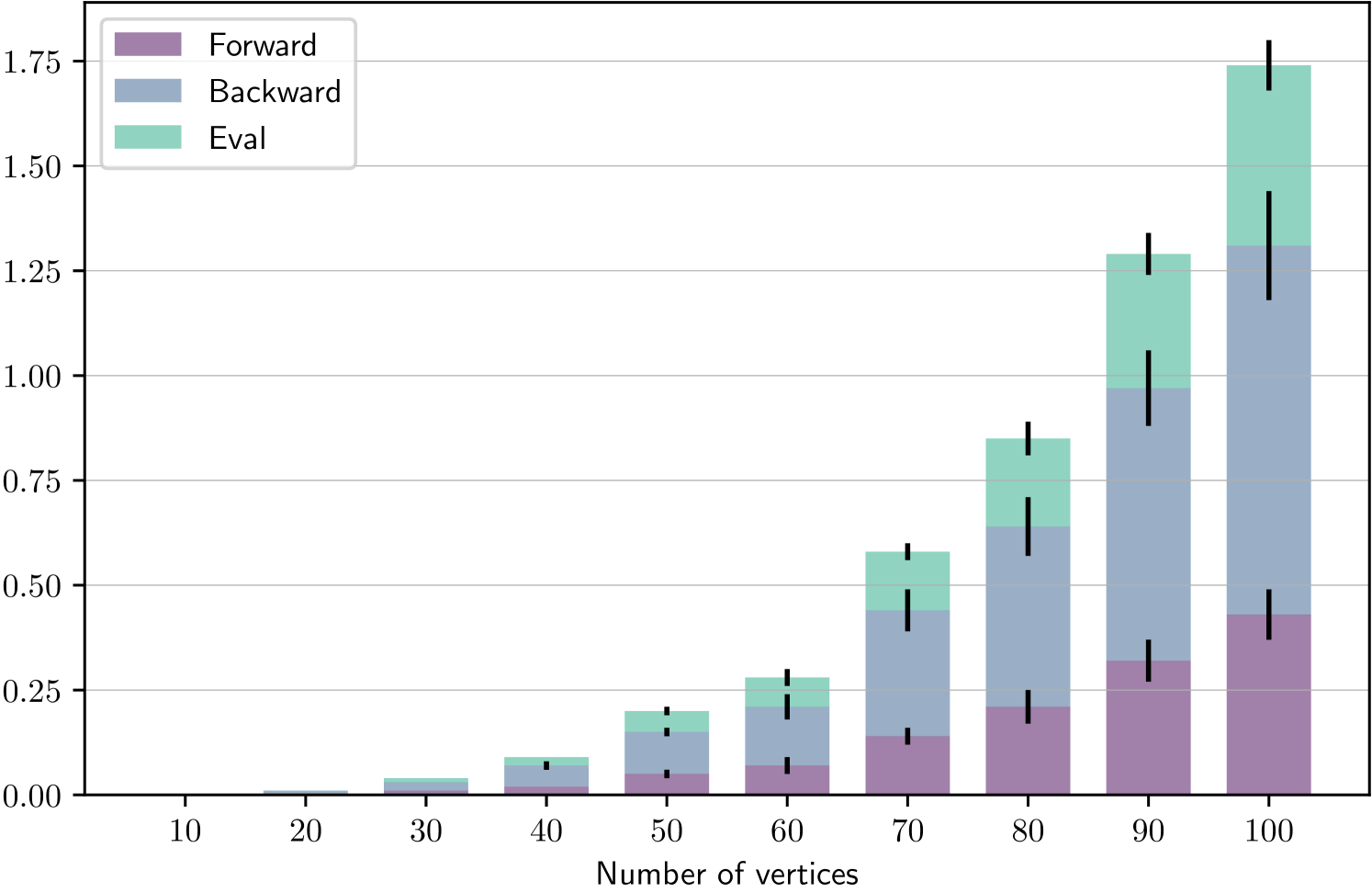
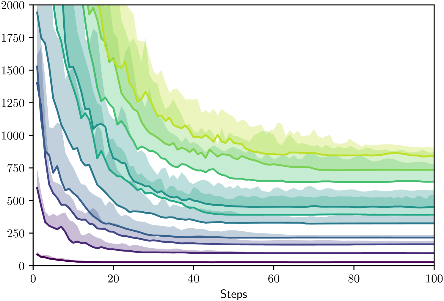
Fig. 4 shows the convergence of values during the optimization process. Here we fix one graph for each number of vertices and run 10 trials each with 120 steps. The colors are assigned to individual graphs, the areas show ranges of the obtained values during the optimization process. The solid lines highlight minimal values.
5.2. Patrolling Airport Gates
One typical application of patrolling is security patrol at airports (see Section 1). Airport buildings have a specific tree structure of terminals with symmetric gates with a central node connecting the terminals. A terminal typically consists of pairs of gates joined by halls. A patrolling graph for an airport with three terminals of 4, 2, and 6 gates is shown in Fig. 5.
We generate a sequence of random airport graphs with 3 terminals and an increasing number of gates determined randomly. Hence, an airport graph with gates has halls and exactly one central node. The gates are targets and have exactly one memory element, while halls and the central node are non-target vertices with memory elements each (thus, the strategy can “remember” the previously visited vertex). The costs of all targets are equal to , and all edges have the same traversal time .
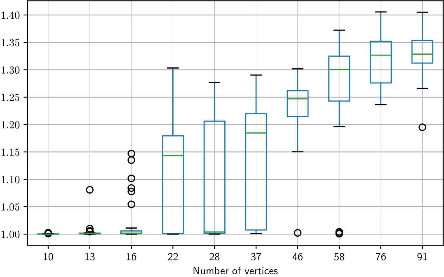
Since the target costs are the same, we can estimate (the achievable protection) by the length of the shortest cycle visiting all targets, which is where is the set of vertices. Note that automatic synthesis of a regular strategy with comparable protection is tricky—the synthesis algorithm must “discover” the relevance of the previously visited vertex and design the memory updates accordingly.
We use the same hyperparameters as above. For each airport, we synthesized 30 strategies, each in 500 steps of iterations. In Fig. 6, we show the protection values of the synthesized strategies for increasing number of vertices normalized by the baseline . For larger , the optimization converges to locally optimal randomized strategies with worse protection than the deterministic-loop strategy. In particular, for , the protection achieved by the constructed strategy is about worse than the baseline on average (with best found strategy loosing above the baseline).
6. Conclusion
The outcomes show that high-quality Defender’s strategies are computed very quickly even for instances of considerable size. Hence, our algorithm can also be used to re-compute a Defender’s strategy dynamically when the patrolling scenario changes.
The problem encountered in our experiments is the existence of locally optimal randomized strategies where the optimization loop gets stuck. An interesting question is whether this problem can be overcome by tuning the parameters of gradient descent or by constructing the initial seeds in a more sophisticated way.
A natural continuation of our study is extending the presented results to scenarios with multiple Defenders and Attackers.
Acknowledgements
Research was sponsored by the Army Research Office and was accomplished under Grant Number W911NF-21-1-0189.
Vít Musil is also supported from Operational Programme Research, Development and Education - Project Postdoc2MUNI (No. CZ.02.2.69/0.0/0.0/18_053/0016952).
Disclaimer
The views and conclusions contained in this document are those of the authors and should not be interpreted as representing the official policies, either expressed or implied, of the Army Research Office or the U.S. Government. The U.S. Government is authorized to reproduce and distribute reprints for Government purposes notwithstanding any copyright notation herein.
References
- (1)
- Agmon et al. (2008a) N. Agmon, S. Kraus, and G. Kaminka. 2008a. Multi-Robot Perimeter Patrol in Adversarial Settings. In Proceedings of ICRA 2008. IEEE Computer Society Press, 2339–2345.
- Agmon et al. (2008b) N. Agmon, V. Sadov, G.A. Kaminka, and S. Kraus. 2008b. The impact of adversarial knowledge on adversarial planning in perimeter patrol. In Proceedings of AAMAS 2008. 55–62.
- Almeida et al. (2004) A. Almeida, G. Ramalho, H. Santana, P. Tedesco, T. Menezes, V. Corruble, and Y. Chevaleyr. 2004. Recent Advances on Multi-Agent Patrolling. Advances in Artificial Intelligence – SBIA 3171 (2004), 474–483.
- An et al. (2014) B. An, E. Shieh, R. Yang, M. Tambe, C. Baldwin, J. DiRenzo, B. Maule, and G. Meyer. 2014. Protect—A Deployed Game Theoretic System for Strategic Security Allocation for the United States Coast Guard. AI Magazine 33, 4 (2014), 96–110.
- Basilico et al. (2009a) N. Basilico, N. Gatti, and F. Amigoni. 2009a. Leader-follower strategies for robotic patrolling in environments with arbitrary topologies. In Proceedings of AAMAS 2009. 57–64.
- Basilico et al. (2012a) N. Basilico, N. Gatti, and F. Amigoni. 2012a. Patrolling Security Games: Definitions and Algorithms for Solving Large Instances with Single Patroller and Single Intruder. Artificial Inteligence 184–185 (2012), 78–123.
- Basilico et al. (2009b) N. Basilico, N. Gatti, T. Rossi, S. Ceppi, and F. Amigoni. 2009b. Extending algorithms for mobile robot patrolling in the presence of adversaries to more realistic settings. In Proccedings of WI-IAT 2009. 557–564.
- Basilico et al. (2010) Nicola Basilico, Nicola Gatti, and Federico Villa. 2010. Asynchronous Multi-Robot Patrolling against Intrusion in Arbitrary Topologies. In Proceedings of AAAI 2010.
- Basilico et al. (2012b) N. Basilico, G. De Nittis, and N. Gatti. 2012b. A Security Game Combining Patrolling and Alarm-Triggered Responses Under Spatial and Detection Uncertainties. In Proceedings of AAAI 2016. 404–410.
- Biswas et al. (2021) A. Biswas, G. Aggarwal, P. Varakantham, and M. Tambe. 2021. Learn to Intervene: An Adaptive Learning Policy for Restless Bandits in Application to Preventive Healthcare. In Proceedings of the International Joint Conference on Artificial Intelligence (IJCAI 2021).
- Bosansky et al. (2011) B. Bosansky, V. Lisy, M. Jakob, and M. Pechoucek. 2011. Computing Time-Dependent Policies for Patrolling Games with Mobile Targets. In Proceedings of AAMAS 2011.
- Brázdil et al. (2018) T. Brázdil, A. Kučera, and V. Řehák. 2018. Solving Patrolling Problems in the Internet Environment. In Proceedings of the International Joint Conference on Artificial Intelligence (IJCAI 2018). 121–127.
- Chen et al. (2017) H. Chen, T. Cheng, and S. Wise. 2017. Developing an Online Cooperative Police Patrol Routing Strategy. Computers, Environment and Urban Systems 62 (2017), 19–29.
- Fang et al. (2013) Fei Fang, Albert Xin Jiang, and Milind Tambe. 2013. Optimal Patrol Strategy for Protecting Moving Targets with Multiple Mobile Resources. In Proceedings of AAMAS 2013.
- Fave et al. (2014) F.M. Delle Fave, A.X. Jiang, Z. Yin, C . Zhang, M. Tambe, S. Kraus, and J. Sullivan. 2014. Game-Theoretic Security Patrolling with Dynamic Execution Uncertainty and a Case Study on a Real Transit System. Journal of Artificial Intelligence Research 50 (2014), 321–367.
- Ford et al. (2014) B. Ford, D. Kar, F.M. Delle Fave, R. Yang, and M. Tambe. 2014. PAWS: Adaptive Game-Theoretic Patrolling for Wildlife Protection. In Proceedings of AAMAS 2014. 1641–1642.
- Ho and Ouaknine (2015) Hsi-Ming Ho and J. Ouaknine. 2015. The Cyclic-Routing UAV Problem is PSPACE-Complete. In Proceedings of FoSSaCS 2015 (Lecture Notes in Computer Science, Vol. 9034). Springer, 328–342.
- Huang et al. (2019) L. Huang, M. Zhou, K. Hao, and E. Hou. 2019. A Survey of Multi-robot Regular and Adversarial Patrolling. IEEE/CAA Journal of Automatica Sinica 6, 4 (2019), 894–903.
- Jakob et al. (2011) M. Jakob, O. Vanek, and M. Pechoucek. 2011. Using Agents to Improve International MaritimeTransport Security. IEEE Intelligent Systems 26, 1 (2011), 90–96.
- Karwowski et al. (2019) J. Karwowski, J. Mandziuk, A. Zychowski, F. Grajek, and B. An. 2019. A Memetic Approach for Sequential Security Games on a Plane with Moving Targets. In Proceedings of AAAI 2019. 970–977.
- Kingma and Ba (2015) Diederik P. Kingma and Jimmy Ba. 2015. Adam: A Method for Stochastic Optimization. In Proceedings of ICLR 2015.
- Klaška et al. (2018) D. Klaška, A. Kučera, T. Lamser, and V. Řehák. 2018. Automatic Synthesis of Efficient Regular Strategies in Adversarial Patrolling Games. In Proceedings of AAMAS 2018. 659–666.
- Klaška et al. (2021) D. Klaška, A. Kučera, V. Musil, and V. Řehák. 2021. Regstar: Efficient Strategy Synthesis for Adversarial Patrolling Games. In Proceedings of UAI 2021.
- Klaška et al. (2020) D. Klaška, A. Kučera, and V. Řehák. 2020. Adversarial Patrolling with Drones. In Proceedings of AAMAS 2020. 629–637.
- Kučera and Lamser (2016) A. Kučera and T. Lamser. 2016. Regular Strategies and Strategy Improvement: Efficient Tools for Solving Large Patrolling Problems. In Proceedings of AAMAS 2016. 1171–1179.
- Maza et al. (2011) I. Maza, F. Caballero, J. Capitán, J.R. Martínez de Dios, and A. Ollero. 2011. Experimental Results in Multi-UAV Coordination for Disaster Management and Civil Security Applications. Journal of Intelligent and Robotic Systems 61, 1–4 (2011), 563–585.
- Munoz de Cote et al. (2013) Enrique Munoz de Cote, Ruben Stranders, Nicola Basilico, Nicola Gatti, and Nick Jennings. 2013. Introducing alarms in adversarial patrolling games: extended abstract. In Proceedings of AAMAS 2013. 1275–1276.
- Norris (1998) J.R. Norris. 1998. Markov Chains. Cambridge University Press.
- Pita et al. (2008) J. Pita, M. Jain, J. Marecki, F. Ordónez, C. Portway, M. Tambe, C. Western, P. Paruchuri, and S. Kraus. 2008. Deployed ARMOR Protection: The Application of a Game Theoretic Model for Security at the Los Angeles Int. Airport. In Proceedings of AAMAS 2008. 125–132.
- Portugal and Rocha (2011) D. Portugal and R. Rocha. 2011. A Survey on Multi-Robot Patrolling Algorithms. Technological Innovation for Sustainability 349 (2011), 139–146.
- Sinha et al. (2018) A. Sinha, F. Fang, B. An, C. Kiekintveld, and M. Tambe. 2018. Stackelberg Security Games: Looking Beyond a Decade of Success. In Proceedings of the International Joint Conference on Artificial Intelligence (IJCAI 2018). 5494–5501.
- Tambe (2011) M. Tambe. 2011. Security and Game Theory. Algorithms, Deployed Systems, Lessons Learned. Cambridge University Press.
- Tsai et al. (2009) J. Tsai, S. Rathi, C. Kiekintveld, F. Ordóñez, and M. Tambe. 2009. IRIS—A Tool for Strategic Security Allocation in Transportation Networks Categories and Subject Descriptors. In Proceedings of AAMAS 2009. 37–44.
- Wang et al. (2019) Y. Wang, Z.R. Shi, L. Yu, Y. Wu, R. Singh, L. Joppa, and F. Fang. 2019. Deep Reinforcement Learning for Green Security Games with Real-Time Information. In Proceedings of AAAI 2019. 1401–1408.
- Xu (2021) L. Xu. 2021. Learning and Planning Under Uncertainty for Green Security. In Proceedings of the International Joint Conference on Artificial Intelligence (IJCAI 2021).
- Yan et al. (2013) Z. Yan, N. Jouandeau, and A.A. Cherif. 2013. A Survey and Analysis of Multi-Robot Coordination. International Journal of Advanced Robotic Systems 10, 12 (2013), 1–18.
- Yin et al. (2010) Z. Yin, D. Korzhyk, C. Kiekintveld, V. Conitzer, and M. Tambe. 2010. Stackelberg vs. Nash in security games: Interchangeability, equivalence, and uniqueness. In Proceedings of AAMAS 2010. 1139–1146.