Minimum-Energy Distributed Filtering^††thanks: This work was supported by the Australian Research Council under Discovery Projects funding scheme (project D0120102152).

There is considerable interest in the literature in multi-agent systems that are capable of performing control and filtering related tasks in a cooperative manner. Applications range from military aerial fleets, monitoring and maintenance agents in industrial applications to biological applications. In this paper, in particular, we are concerned with distributed filtering using a network of filters that estimate the state of a plant using disturbance contaminated local measurements. An interesting case is when these filters individually have difficulty providing an accurate and complete estimate of the plant, a problem that is resolved by using information from the neighbouring filters.

Kalman filtering is the focus of many of the existing methods proposed for distributed filtering. An early result on this subject by Durrant-Whyte et. al [1, 2] provides an exact decentralized formulation for the multi-sensor version of the Kalman filter. This formulation avoids the requirement of a central processing or communication unit with which each sensor has to communicate its information for calculating the state estimate of the plant. The decentralized scheme is robust to sensor failure and network changes, reduces the communication load and allows for faster information processing. The decentralized Kalman filter proposed in [1, 2] however, requires an all-to-all communication of state error information and variance error information between the sensors; this impairs its scalability to bigger networks. Olfati-Saber [3] proposed a distributed Kalman filter algorithm that involves two additional consensus filters which are needed for fusion of the sensor information and covariance information required for the decentralized Kalman filtering scheme used. The distributed naming refers to the fact that all-to-all information sharing is avoided and instead each agent only shares information with its local neighbors. The distributed consensus algorithms proposed in [3] assume disturbance free data sharing between the sensors that is arguably an unrealistic assumption in applications involving imperfect communication.

More recently, observer designs based on linear matrix inequalities (LMIs) have been employed to tackle the imperfect communication problem in multi-agent distributed estimation [4, 5]. Subbotin and Smith [5] proposed a convex optimization problem where minimizing the estimation error covariance of the global network selects the local observer gains. Ugrinovskii [4] designed the observer gains by minimizing an $H_{\infty}$ consensus performance cost that guarantees the associated disturbance attenuation criterion and guarantees the convergence of the filter dynamics of the nodes. Both works target the asymptotic performance of their respective estimation algorithms by using constant gains. This is in contrast to filtering algorithms that use time-varying gains calculated to adjust both the transient and the asymptotic performance  [6].

In this paper a minimum-energy distributed filtering algorithm is proposed that addresses the imperfect communication of the nodes by locally minimizing a quadratic energy cost comprising the initialization and measurement errors as well as the communication errors of the local filter. A novel contribution of this paper that leads to the distributed nature of the local filters lies in augmenting the minimum-energy cost functional with a cost on approximating the neighboring estimates. Furthermore, a penalty is included in the local costs that provides a guaranteed $H_{\infty}$ disturbance attenuation property over the network of filters.

We provide a condition on the network parameters that is sufficient to ensure convergence of the proposed filters. The condition is quite general, and captures the types of convergence considered in [4, 5] as special cases. Moreover, we offer a tuning algorithm based on LMIs that facilitates the implementation of the proposed filters with guaranteed $H_{\infty}$ performance and convergence of the filters. A simulation example regarding the Chua electronic circuit [7] is provided that demonstrates the effectiveness of the proposed algorithm in the case of a chaotic plant system and network of five filters that estimate the state of the plant.

The remainder of the paper is organised as follows. Section II reviews the concept of minimum-energy filtering. In Section III we extend the minimum-energy filtering paradigm to allow for a distributed filtering formulation as well as to impose the $H_{\infty}$ filtering performance criterion. The distributed minimum-energy filter is provided in that section. Convergence of the proposed filter is studied in Section IV, and tuning of the filter is discussed in Section V. Section VI illustrates the design procedure and performance of the proposed filter via simulation, and Section VII concludes the paper.

In this section we review the concept of minimum-energy filtering that was pioneered by Mortensen [8] and was further elaborated by Hijab [9]. Later, we use this method to obtain a distributed filtering algorithm for estimating the state of a linear system using a network of filters. Consider the linear system

$$\dot{x}=Ax+Bw,\quad x(0)=x_{0},$$

(1)

where the signals $x\in\mathbb{R}^{n}$ and $w\in\mathbb{R}^{m}$ are, respectively, the state and the unknown modeling disturbance; the latter is assumed to be $\mathcal{L}_{2}$ integrable on $[0,T]$. The matrices $A\in\mathbb{R}^{n\times n}$ and $B\in\mathbb{R}^{n\times m}$ are known state matrix and input disturbance coefficient matrix, respectively. Note that $x_{0}$ is assumed to be unknown.

Further consider the following measurement model

$$y=Cx+Dv,$$

(2)

where the signals $y,v\in\mathbb{R}^{p}$ are the measured data and the unknown measurement disturbance, which is also assumed to be $\mathcal{L}_{2}$ integrable on $[0,T]$. The matrices $C\in\mathbb{R}^{p\times n}$ and $D\in\mathbb{R}^{p\times p}$ are the measurement matrix and the measurement disturbance coefficient matrix, receptively, that are assumed to be known from the model. Denote $Q\triangleq BB^{\top}$ and $R\triangleq DD^{\top}$ and assume that $R>0$.

Associated with these equations is the energy functional measuring the aggregated energy associated with the unknowns $(x_{0},w,v)$,

$$J_{t}=\frac{1}{2}\|x_{0}-\xi\|_{\mathcal{X}}^{2}+\frac{1}{2}\int_{0}^{t}\left(\|w\|^{2}+\|v\|^{2}\right)d\tau,$$

(3)

where $\|a\|_{A}\triangleq a^{\top}Aa$, the matrix $\mathcal{X}\in\mathbb{R}^{n\times n}$ is a weighting on the difference between the unknown initial state and its nominated a priori estimate $\xi$.

Denote by $y_{[0,t]}$ the data obtained according to (2) during the time $[0,t]$. Given the measurement data $y_{[0,t]}$, minimizing the cost (3) with respect to $w$ and $x(0)$, subject to equations (1) and (2), leads to an optimal state trajectory $x^{*}_{[0,t]}$. This is the ‘most likely trajectory’ [8] or the minimum-energy trajectory that is compatible with the data $y_{[0,t]}$. The end point of this trajectory constitutes the minimum-energy estimate of the state $x(t)$, given the measurement data $y_{[0,t]}$,

$$\hat{x}(t)\triangleq x^{*}_{[0,t]}(t),\quad t\in[0,T].$$

(4)

It is desirable to obtain the estimates $\hat{x}(t)$ continuously as time evolves in $[0,T]$. Note that in general, for $0\leq t_{1}<t_{2}\leq T$,

$$\hat{x}(t_{1})=x^{*}_{[0,t_{1}]}(t_{1})\not=x^{*}_{[0,t_{2}]}(t_{1}).$$

(5)

Therefore, it is not sufficient to only minimize the cost (3) over $[0,T]$ and infinite sequence of minimizations are required if all the estimated values in this period are needed. The calculus of variations can be utilized to solve this problem and obtain a recursive filtering algorithm similar to those arising in optimal control [10]. The idea is to solve the following two step optimization problem

$$\begin{split}\inf_{x(0)}(\inf_{w}J_{t})=&\inf_{x(0)}\left[\frac{1}{2}\|x(0)-\xi\|_{\mathcal{X}}^{2}\right.\\ &+\left.\inf_{w}\frac{1}{2}\int_{0}^{t}(\|w\|^{2}+\|y-Cx\|_{R^{-1}}^{2})d\tau\right].\end{split}$$

(6)

The inner minimization problem is solved as an optimal tracking problem, in which the system (1) is to track the given output signal $y(\tau)$, $\tau\in[0,t]$, and $w$ is treated as a control input signal. For this step both $x(0)$ and $x(t)=x$ are considered to be fixed but constrained by (1) for $0\leq\tau\leq t$. The associated value function of this inner tracking problem, encoding the minimum energy required to take the system from the initial state $x(0)$ to the state $x$ over the time period $[0,t]$, is

$$V(x,t)=\min_{w}J_{t},$$

(7)

which from (3) has the initial condition

$$V(x,0)=\frac{1}{2}\|x-\xi\|_{\mathcal{X}}^{2}.$$

(8)

Note that in (7), the variables $x$ and $t$ are considered as independent variables. That is, by selecting a time $t$ and an end state $x$, the value function (7) provides the optimal value arising from minimizing the cost (3) over $w$.

The final step is to perform the outer minimization, which is equivalent to minimizing the value function over $x$. This leads to the optimal trajectory $x^{*}$ and the minimum-energy estimate chosen as its final value, $\hat{x}(t)=x^{*}(t)$. Provided the value function is sufficiently smooth, this can be achieved by solving

$$\nabla_{x}V(x,t)=0.$$

(9)

Mortensen [8] proposed solving the next equation, obtained from (9), that leads to a recursive set of equations for updating $\hat{x}(t)$.

$$\dfrac{d}{dt}\{\nabla_{x}V(x,t)\}=0.$$

(10)

The resulting filter turns out to be in the exact form of the Kalman-Bucy filter [6]. While the resulting filter is well-known in the literature, the minimum-energy methodology is less known. Nevertheless, minimum-energy filtering is a systematic recursive method that can be applied in many applications including in distributed filtering considered in the rest of this paper.

Consider a network of $N$ filters with a directed graph topology $\mathbf{G}=(\mathbf{V},\mathbf{E})$ where $\mathbf{V}$ and $\mathbf{E}\subseteq\mathbf{V}\times\mathbf{V}$ are the set of vertices and the set of edges, respectively. An edge directing node $j$ of the graph $\mathbf{G}$ towards node $i$ where $i,j\in\{1,\cdots,N\}$ is denoted by $(i,j)$. In accordance with the common convention [3], the graph $\mathbf{G}$ is assumed to have no self-loops, i.e., $(i,i)\notin\mathbf{E}$. The neighborhood of node $i$, i.e., the set of nodes which send information to node $i$, is denoted by $\mathcal{N}_{i}=\{j:(i,j)\in\mathbf{E}\}$.

In this section we again consider the plant model (1). As in Section II, the initial state $x_{0}$ and the $\mathcal{L}_{2}$-integrable modeling error $w$ are unknown. Our goal is to construct a network of filters that can each estimate the plant state $x$ using the measurements of the following type,

$$y_{i}=C_{i}x+D_{i}v_{i},$$

(11)

where $i=1,2,\cdots,N$, indicates the $i$th node of the network. Each measurement $y_{i}\in\mathbb{R}^{p}$ is obtained using the associated observation matrix $C_{i}\in\mathbb{R}^{p\times n}$ known to node $i$ from the model. The signal $v_{i}\in\mathbb{R}^{p}$ is an unknown measurement error assumed to be $\mathcal{L}_{2}$ integrable on $[0,T]$, with known coefficient matrices $D_{i}\in\mathbb{R}^{p\times p}$ such that the matrix $R_{i}\triangleq D_{i}D_{i}^{\top}$ is positive definite.

In addition, the filter $i$ obtains information from $l_{i}$ agents in its neighbourhood $\mathcal{N}_{i}$; $l_{i}$ is the cardinality of the set $\mathcal{N}_{i}$, $0\leq l_{i}\leq N$. The obtained signals at node $i$ are

$$c_{ij}=W_{ij}\hat{x}_{j}+F_{ij}\epsilon_{ij},\quad j\in\mathcal{N}_{i},$$

(12)

where $\hat{x}_{j}$ is the estimate of state $x$ at node $j\in\mathcal{N}_{i}$. Similar to the measurements $y_{i}$, the signals $c_{ij}\in\mathbb{R}^{m}$ are obtained using the weighted connectivity matrices $W_{ij}\in\mathbb{R}^{m\times n}$ that are assumed to be known to node $i$ while $\hat{x}_{j}$ are not known. The signals $\epsilon_{ij}\in\mathbb{R}^{m}$ are unknown communication errors of class $\mathcal{L}_{2}[0,T]$, with known coefficient matrices $F_{ij}\in\mathbb{R}^{m\times m}$ such that $S_{ij}\triangleq F_{ij}F_{ij}^{\top}$ are positive definite.

In many existing methodologies, cf. [4, 7, 5], treating communications between the nodes as extra measurements results in observer design conditions that require solving large-scale coupled matrix equations or matrix inequalities. In contrast, we invoke the following equation that is going to be instrumental in obtaining decoupled filter gain conditions. Since $\hat{x}_{j}$ are meant to represent the state vector $x$ with high fidelity, we use the following model at node $i$,

$$\hat{x}_{j}=x+\eta_{ij}.$$

(13)

The signals $\eta_{ij}\in\mathbb{R}^{b}$ denote the unknown error signals of this assignment. Note that this model is only proposed for node $i$ and node $j$ obviously computes $\hat{x}_{j}$ using its corresponding filter.

Next, we pose a minimum-energy filtering problem to obtain a distributed filter at each node $i$ such that a cost functional, depending on the unknown initial state of the plant $x_{0}$ and the unknown errors in the measurements and neighbouring information associated to filter $i$, is minimized. This cost functional is in fact the sum of aggregated energies in the unknowns of the model, the measurements and the neighbouring information associated with filter $i$. Note that the distributed estimation paradigm restricts us to only utilizing local measurements $y_{i}$ and local information from the neighboring nodes, i.e. $c_{ij},\;j\in\mathcal{N}_{i}$ in this optimization process. It is important to stress the role of the unknown signals $\eta_{ij}$ that are also to be optimized over in this process.

The idea behind minimizing the cost functional over $\eta_{ij}$, $j\in\mathcal{N}_{i}$, amounts to agent $i$ relying on the fact that its neighboring agents are also minimum-energy type estimators of the plant state and hence their estimates can be thought of as estimates of the plant state contaminated with errors that are based on minimum-energy filtering too. This is a key idea among the results of this work that facilitates obtaining a distributed solution for our problem. The concept of minimum-energy filtering was explained in details in Section II.

The energy cost similar to (3), associated with the system (1), the information available to node $i$ according to (11) and (12), and the approximation model (13) is defined as

$$\begin{split}&\frac{1}{2}\|x_{0}-\xi_{i}\|_{\mathcal{X}_{i}}^{2}+\frac{1}{2}\int_{0}^{t}\bigg{(}\|w\|^{2}+\|v_{i}\|^{2}\\ &\qquad\qquad\qquad+\sum_{j\in\mathcal{N}_{i}}(\|\epsilon_{ij}\|^{2}+\|\eta_{ij}\|^{2}_{Z^{-1}_{ij}})\bigg{)}d\tau,\end{split}$$

(14)

where the signal $\xi_{i}$ is an a priori candidate for the initial state $x_{0}$ at node $i$ and the matrix $\mathcal{X}_{i}$ is an a priori known weighting for the initialization error $x_{0}-\xi_{i}$. The weighting matrices $Z_{ij}=Z_{ij}^{\prime}>0$, $Z_{ij}\in\mathbb{R}^{n\times n}$, quantify the ‘confidence’ of node $i$ in the quality of its neighbor estimates $\hat{x}_{j}$ and are selected locally by node $i$.

Given the measurement data $y_{i}|_{[0,t]}$ and the communication data $c_{ij}|_{[0,t]}$, the signals $v_{i}$ and $\epsilon_{ij}$ are identified as dependent variables and the energy cost functional (14) has arguments $x_{0}$, $w_{i}$ and $\;\eta_{ij}$. Next, based on (14) define the following cost functional for node $i$

	$\displaystyle J_{i,t}(x_{0},w,\{\eta_{ij}\})=\frac{1}{2}\|x_{0}-\xi_{i}\|_{\mathcal{X}_{i}}^{2}+\frac{1}{2}\int_{0}^{t}\bigg{(}\|w\|^{2}$
	$\displaystyle\quad+\|y_{i}-C_{i}x\|^{2}_{R_{i}^{-1}}+\sum_{j\in\mathcal{N}_{i}}(\|c_{ij}-W_{ij}x-W_{ij}\eta_{ij}\|^{2}_{S_{ij}^{-1}}$
	$\displaystyle\quad+\|\eta_{ij}\|^{2}_{Z^{-1}_{ij}}-\|x-\hat{x}_{i}\|^{2}_{M_{i}^{-1}})\bigg{)}d\tau,$		(15)

where the matrix $M_{i}>0\in\mathbb{R}^{n\times n}$ is a given coefficient. The selection of this matrix will be discussed in Section V. The inclusion of the error term $\int_{0}^{t}\|x-\hat{x}_{i}\|^{2}_{M_{i}^{-1}}d\tau$ with a negative sign enforces a guaranteed $H_{\infty}$ type performance at node $i$ while a minimum-energy estimate is sought [12].

The principle of minimum energy requires that a set of the unknowns $(x_{0},w,\eta_{ij})$, $j\in\mathcal{N}_{i}$, be sought at each node $i$ that are compatible with the measurements $y_{i}$ and the neighbourhood information $c_{ij}$ in satisfying (11), (12) and (13) while minimizing the cost (15),

$$\inf_{x}\;\inf_{w,\;\eta_{ij}}J_{i,t}(x_{0},w,\eta_{ij}),$$

(16)

where $x=x(t)$. Using the minimum energy filtering approach as was explained in Section II the following filter is obtained

	$\displaystyle\dot{\hat{x}}_{i}$	$\displaystyle=$	$\displaystyle A\hat{x}_{i}+K_{i}^{-1}\bigg{(}C_{i}^{\top}R^{-1}(y_{i}-C_{i}\hat{x}_{i})$		(17)
		$\displaystyle+$	$\displaystyle\sum_{j\in\mathcal{N}_{i}}W_{ij}^{\top}U^{-1}_{ij}(c_{ij}-W_{ij}\hat{x}_{i})\bigg{)},\quad\hat{x}_{i}(0)=\xi_{i}.$

The matrix $U_{ij}$ is defined as $U_{ij}\triangleq S_{ij}+W_{ij}Z_{ij}W_{ij}^{\top}$. The positive definite time-varying gain matrix $K_{i}$ is calculated from the following Riccati equation

	$\displaystyle\dot{K}_{i}$	$\displaystyle=$	$\displaystyle-K_{i}QK_{i}+C_{i}^{\top}R_{i}^{-1}C_{i}+\sum_{j\in\mathcal{N}_{i}}W_{ij}^{\top}U^{-1}_{ij}W_{ij}$		(18)
			$\displaystyle-M_{i}^{-1}-A^{\top}K_{i}-K_{i}A,$
	$\displaystyle\quad K_{i}(0)$	$\displaystyle=$	$\displaystyle\mathcal{X}_{i}.$

The matrix $Q$ is defined as $Q\triangleq BB^{\top}$ where $B$ was given in (1).

An advantage of equation (18) is that it does not depend on any measurements, neighbour information or any on-line acquired data and hence can be fully solved off-line. It can also be solved on-line forward in time, so that the computed values for $K_{i}(t)$ can be used to dynamically run the observer (17). Also, the filter equation (17) has the standard form of a distributed filter that produces state estimates based on local measurements and information obtained about the neighbours. A noteworthy feature of the proposed filter is that its gains are dependent only on the information available at node $i$. The only matrix to be computed to find the gains, the matrix $K_{i}$ is computed locally, without interacting with the neighbours, provided the matrices $M_{i}$ are defined a priori. This feature of the proposed minimum energy estimator sets it apart from other distributed estimation algorithms such as those proposed in [4, 5].

In this section we provide sufficient conditions to guarantee that the interconnected network of filters designed according to equations (17) and (18) converges to the true state of the plant as $t\to\infty$. Due to the presence of uncertainty, the convergence is understood in the $H_{\infty}$ sense. Firstly, we show that error dynamics exhibit properties of an internally stable system. The notion of internal stability is equivalent to asymptotic convergence of the estimation error of the network in the absence of disturbance signals. Secondly, we will show that when disturbances are $\mathcal{L}_{2}$ integrable on $[0,\infty)$, the filter ensures disturbance attenuation properties similar to those of an $H_{\infty}$ filter.

Consider the node error $e_{i}\triangleq\hat{x}_{i}-x$ and its dynamics,

	$\displaystyle\hskip-21.52771pt\dot{e}_{i}=Ae_{i}-Bw$
	$\displaystyle\hskip-10.76385pt-K_{i}^{-1}\bigg{(}(C_{i}^{\top}R_{i}^{-1}C_{i}+\sum_{j\in\mathcal{N}_{i}}W_{ij}^{\top}U^{-1}_{ij}W_{ij})e_{i}$
	$\displaystyle\hskip-10.76385pt-C_{i}^{\top}R^{-1}_{i}D_{i}v_{i}-\sum_{j\in\mathcal{N}_{i}}W_{ij}^{\top}U^{-1}_{ij}(W_{ij}e_{j}+F_{ij}\epsilon_{ij})\bigg{)},$		(19)

where the dynamics of the matrix $K_{i}$ are given in (18).

Let us introduce the following notation

$$\begin{split}&e\triangleq[e_{1}^{\top},\ldots,e_{N}^{\top}]^{\top},\\ &\tilde{A}\triangleq I_{N}\otimes A,\quad C\triangleq\mbox{diag}[C_{1},\ldots,C_{N}],\quad\tilde{Q}\triangleq I_{N}\otimes Q,\\ &R\triangleq\mbox{diag}[R_{1},\ldots,R_{N}],\quad K\triangleq\mbox{diag}[K_{1},\ldots,K_{N}],\\ &M\triangleq\mbox{diag}[M_{1},\ldots,M_{N}],\\ &\Delta\triangleq\mbox{diag}[\sum_{j\in\mathcal{N}_{1}}W_{1j}^{\top}U^{-1}_{1j}W_{1j},\ldots,\sum_{j\in\mathcal{N}_{N}}W_{Nj}^{\top}U^{-1}_{Nj}W_{Nj}],\\ &\tilde{\Delta}\triangleq\mbox{diag}[\sum_{j\in\mathcal{N}_{1}}W_{1j}^{\top}U^{-1}_{1j}W_{1j}Z_{1j}W_{1j}^{\top}U^{-1}_{1j}W_{1j},\ldots,\\ &\quad\quad\quad\sum_{j\in\mathcal{N}_{N}}W_{Nj}^{\top}U^{-1}_{Nj}W_{Nj}Z_{Nj}W_{Nj}^{\top}U^{-1}_{Nj}W_{Nj}],\\ &\tilde{L}\triangleq[L_{ij}],\\ &L_{ij}=\begin{cases}\sum_{j\in\mathcal{N}_{i}}W_{ij}^{\top}U_{ij}^{-1}W_{ij}Z_{ij}W_{ij}^{\top}U_{ij}^{-1}W_{ij},\\ &\hskip-56.9055pti=j,\\ -W_{ij}^{\top}U^{-1}_{ij}W_{ij},&\hskip-56.9055pti\neq j,\ j\in\mathcal{N}_{i},\\ 0,&\hskip-56.9055pti\neq j,\ j\not\in\mathcal{N}_{i},\end{cases}\end{split}$$

(20)

where $\mbox{diag}[X_{1},\ldots,X_{N}]$ denotes the block diagonal matrix with $X_{1},\ldots,X_{N}$ as its diagonal blocks, and $\otimes$ is the Kronecker product of matrices. Using this notation, $K$ satisfies the differential Riccati equation

	$\displaystyle\dot{K}$	$\displaystyle=$	$\displaystyle-K\tilde{Q}K+C^{\top}R^{-1}C+\Delta-M^{-1}$		(21)
			$\displaystyle-\tilde{A}^{\top}K-K\tilde{A},$
	$\displaystyle K(0)$	$\displaystyle=$	$\displaystyle\mbox{diag}[\mathcal{X}_{1},\ldots,\mathcal{X}_{N}].$

The following theorem is the main result of this paper, which characterizes $H_{\infty}$ performance of the distributed minimum energy filter (17).

The proof is omitted due to page restrictions.

Several special cases of Theorem 1 deserve attention.

Theorem 1 provides a sufficient condition guaranteeing the convergence in the $H_{\infty}$ sense of the network of filters consisting of the estimators (17), (18). To apply this condition the matrices $M_{i}$ need to be selected to satisfy (22). The following propositions are instrumental in designing these matrices. First, we recall a connection between the differential Riccati equation (18) and a corresponding algebraic Riccati equation (ARE) [13],

	$\displaystyle Z_{i}A^{\top}+AZ_{i}$	$\displaystyle-$	$\displaystyle Z_{i}(C_{i}^{\top}R_{i}^{-1}C_{i}$		(26)
		$\displaystyle+$	$\displaystyle[\Delta]_{ii}-M_{i}^{-1})Z_{i}+BB^{\top}=0.$

Next, we use the above connection between the ARE (26) and the differential Riccati equation (18) to derive a tractable sufficient condition for the conditions of Theorem 1 to hold.

In the light of Theorem 2, solving the LMI (30) in variables $X_{i}$, $M_{i}^{-1}$, $P$ is considered as a tuning process for the proposed filtering algorithm (17), (18). Tuning can be carried out, e.g., using MATLAB. It can be performed assuming the matrix $P$ is given, to obtain the matrices $M_{i}^{-1}$ and $\mathcal{X}_{i}$ to be used in equation (18). According to Theorem 1, this tuning process will guarantee the disturbance attenuation and the internal stability of the error dynamics for the entire networked filter consisting of the node filters (17), (18). Alternatively, the matrices $M_{i}$, $i=1\ldots,N$, can be selected a priori. The filter gain equations (18) are completely decoupled in this case, and Theorem 2 can be used to compute the matrix $P$ to characterize performance of the corresponding distributed filter (17).

In this section, a simulated network of five sensor nodes is considered that are to estimate a three-dimensional plant. The plant’s state matrix is given by

$$A=\left[\begin{array}[]{ccc}-3.2&10&0\\ 1&-1&1\\ 0&-14.87&0\\ \end{array}\right].$$

(31)

This corresponds to a Chua electronic circuit which was considered in [7]. A Chua circuit is a chaotic system switching between three regimes of operation. Here, we focus on one of the regimes and consider the second mode of the Chua example that was considered in [7]. The $C_{i}$ matrices considered are $C_{1}=C_{4}=0.001[3.1923~−4.6597~1]$ and $C_{2}=C_{3}=C_{5}=[−0.8986~0.1312~−1.9703]$. The network considered consists of five nodes with connectivity edges $E=\{(1,3),(2,3),(3,1),(3,2),(3,4),(4,3),(4,5),(5,4)\}$. Following [7], all communication matrices associated with the sensor nodes $i$ and $j$ are taken to be $W_{ij}=I_{3\times 3}$ if the pair $(i,j)$ belongs to the set of edges $E$, and otherwise $W_{ij}=0_{3\times 3}$.

We have considered the remainder of the coefficient matrices to be $B=0.4I_{3\times 3}$, $D_{i}=0.025I_{1\times 3}$ and $F_{ij}=0.5I_{3\times 3}$. The measure of confidence in the neighbouring estimates is set to be $Z_{ij}=0.1I_{3\times 3}$. The initial values for the Riccati differential equations (18) are chosen to be $K_{i}(0)=10I_{3\times 3}$ and the matrix $M^{-1}$ is chosen by solving (30) with the disturbance attenuation weighting matrix $P=\frac{1}{2}(\mathcal{L}+\mathcal{L}_{\top})\otimes I$ (to ensure (30) holds strictly, in fact we solved (30) with $P=\frac{1}{2}(\mathcal{L}+\mathcal{L}_{\top})\otimes I+0.01I$). According to Theorem 2, this guarantees the satisfaction of the conditions of Theorem 1. Furthermore, with this choice of matrix $P$, the proposed minimum energy filter guarantees that estimation error dynamics are internally stable and exhibit the $H_{\infty}$ performance expressed in condition (25).

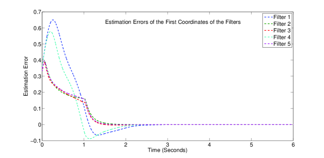
To illustrate performance of the filters, they are simulated using MATLAB. The simulation was implemented with the maximum step size of $0.001$ seconds and simulation time of $10$ seconds. The system disturbances are modeled as pulse signals of appropriate dimensions that last for $1$ seconds. The initial state is drawn from a normally distributed vectors with mean of $0.1$ and standard deviation $0.2$. Figure 1 shows the plot of the estimation error of the first coordinate of each filter, $\hat{x}^{1}_{i}(t)-x^{1}(t)$. The plots confirm that despite some of local filters alone lead to an undetectable estimation problem, the proposed distributed filter has successfully utilized imperfect communications between the nodes to provide estimates at each node with estimation errors converging to zero.

In this paper we proposed a distributed filtering algorithm by utilizing an $H_{\infty}$ minimum-energy filtering approach. The algorithm employs a decoupled computation of the individual filter coefficients. This is achieved by considering the estimation error of neighbouring agents as additional exogenous disturbances weighted according to the nodes’ confidence in their neighbours’ estimates. The proposed algorithm is shown to provide guaranteed internal stability and desired disturbance attenuation of the network error dynamics. The paper has discussed tuning of the algorithm. We have also provided a simulation example that confirms convergence of the proposed algorithm in the case a Chua circuit with undetectable pairs $(A,C_{i})$ at some of the nodes.

References

- [1] H. F. Durrant-Whyte, B. Rao, and H. Hu, “Toward a fully decentralized architecture for multi-sensor data fusion,” in Robotics and Automation, 1990. Proceedings., 1990 IEEE International Conference on. IEEE, 1990, pp. 1331–1336.
- [2] B. Rao, H. Durrant-Whyte, and J. Sheen, “A fully decentralized multi-sensor system for tracking and surveillance,” The International Journal of Robotics Research, vol. 12, no. 1, pp. 20–44, 1993.
- [3] R. Olfati-Saber, “Distributed kalman filter with embedded consensus filters,” in Decision and Control, 2005 and 2005 European Control Conference. CDC-ECC’05. 44th IEEE Conference on. IEEE, 2005, pp. 8179–8184.
- [4] V. Ugrinovskii, “Distributed robust filtering with h-infinity consensus of estimates,” Automatica, vol. 47, no. 1, pp. 1–13, 2011.
- [5] M. V. Subbotin and R. S. Smith, “Design of distributed decentralized estimators for formations with fixed and stochastic communication topologies,” Automatica, vol. 45, no. 11, pp. 2491 – 2501, 2009.
- [6] B. D. O. Anderson and J. Moore, Optimal filtering. Prentice Hall, 1979.
- [7] V. Ugrinovskii, “Distributed robust estimation over randomly switching networks using consensus,” Automatica, vol. 49, no. 1, pp. 160 – 168, 2013.
- [8] R. E. Mortensen, “Maximum-likelihood recursive nonlinear filtering,” Journal of Optimization Theory and Applications, vol. 2, no. 6, pp. 386–394, 1968.
- [9] O. B. Hijab, “Minimum energy estimation,” Ph.D. dissertation, University of California, Berkeley, 1980.
- [10] M. Athans and P. Falb, Optimal control: an introduction to the theory and its applications. McGraw-Hill, 1966.
- [11] V. Ugrinovskii, “Conditions for detectability in distributed consensus-based observer networks,” IEEE Tran. Autom. Contr., vol. 58, pp. 2659 – 2664, 2013, arXiv:1303.6397[cs.SY].
- [12] W. M. McEneaney, “Robust filtering for nonlinear systems,” Systems & control letters, vol. 33, no. 5, pp. 315–325, 1998.
- [13] T. Başar and P. Bernhard, H [infinity symbol]-optimal control and related minimax design problems: A dynamic game approach. Birkhčauser (Boston), 1995.