This paper was converted on www.awesomepapers.org from LaTeX by an anonymous user.
Want to know more? Visit the Converter page.

Mixed effects models for extreme value index regression

Koki Momoki1 and Takuma Yoshida2

1,2Graduate School of Science and Engineering, Kagoshima University
1-21-40 Korimoto, Kagoshima, Kagoshima, 890-8580, Japan
E-mail: k3499390@kadai.jpE-mail: yoshida@sci.kagoshima-u.ac.jp
Abstract

Extreme value theory (EVT) provides an elegant mathematical tool for the statistical analysis of rare events. When data are collected from multiple population subgroups, because some subgroups may have less data available for extreme value analysis, a scientific interest of many researchers would be to improve the estimates obtained directly from each subgroup. To achieve this, we incorporate the mixed effects model (MEM) into the regression technique in EVT. In small area estimation, the MEM has attracted considerable attention as a primary tool for producing reliable estimates for subgroups with small sample sizes, i.e., “small areas.” The key idea of MEM is to incorporate information from all subgroups into a single model and to borrow strength from all subgroups to improve estimates for each subgroup. Using this property, in extreme value analysis, the MEM may contribute to reducing the bias and variance of the direct estimates from each subgroup. This prompts us to evaluate the effectiveness of the MEM for EVT through theoretical studies and numerical experiments, including its application to the risk assessment of a number of stocks in the cryptocurrency market.


Keywords: Extreme value index regression; Extreme value theory; Mixed effects model; Pareto-type distribution; Risk assessment

1 Introduction

Statistical analysis of rare events is crucial for risk assessment in various fields, including meteorology, environment, seismology, finance, economics and insurance. Extreme value theory (EVT) provides an elegant mathematical tool for the analysis of rare events.

In the framework of univariate EVT, the generalized extreme value distribution (see, Fisher and Tippett 1928; Gumbel 1958) and generalized Pareto distribution (GPD, see, Davison and Smith 1990) are standard models for fitting extreme value data. In addition, the class of GPDs with unbounded tails is called the Pareto-type distribution, which has been recognized as an important model for analyzing heavy-tailed data (see, Beirlant et al. 2004). As an important direction of development in EVT, these models have been extended to regression models to incorporate covariate information into extreme value analysis (see, Davison and Smith 1990; Beirlant and Goegebeur 2003; Beirlant et al. 2004; Wang and Tsai 2009). However, few regression techniques have been developed for unit-level data in extreme value analysis.

The data category of interest is denoted by {(Yij,𝑿ij),i=1,2,,nj,j=1,2,,J}\{(Y_{ij},{\bm{X}}_{ij}),\ i=1,2,\ldots,n_{j},\ j=1,2,\ldots,J\}, where JJ is the number of population subgroups, njn_{j} is the sample size from the jjth population subgroup, YijY_{ij} is the response of interest, and 𝑿ij{\bm{X}}_{ij} is the vector of relevant covariates. In much of the literature on small area estimation (SAE), this data category is referred to as unit-level data, and each subgroup is then called an “area” (see, Rao and Molina 2015; Sugasawa and Kubokawa 2020; Molina, Corral, and Nguyen 2022). In particular, an area with a small sample size is the so-called “small area,” which is described in detail by Jiang (2017). Examples of an area include a geographic region such as a state, county or municipality, or a demographic group such as a specific age-sex-race group. From the definition on p. 173 of Rao and Molina (2015), unit-level data means that the number of areas JJ is known, and each observation (Yij,𝑿ij)(Y_{ij},{\bm{X}}_{ij}) is explicitly assigned to one of the areas. This study aims to develop the regression technique of extreme value analysis for unit-level data.

Our purpose is not to pool data from multiple areas into a single area by clustering, nor to create a new set of areas with heterogeneous characteristics (see, Bottolo et al. 2003; Rohrbeck and Tawn 2021; de Carvalho, Huser, and Rubio 2023; Dupuis, Engelke, and Trapin 2023 and references therein). Unlike these approaches, our goal is to enhance the accuracy of extreme value analysis by using information from all areas simultaneously, instead of building models by area. However, if the heterogeneity between all areas is modeled as parameters, the number of parameters depends on the number of areas JJ. Accordingly, for large JJ, the fully parametric model can lead to a large bias in the parameter estimates (see, Section 4 of Ruppert, Wand, and Carroll 2003; Broström and Holmberg 2011). Thus, we want to develop a model for extreme value analysis that does not require many parameters for unit-level data. To this end, we incorporate the mixed effects model (MEM) into EVT. The MEM has been described in Jiang (2007), Wu (2009), Jiang (2017), and references therein. This model captures the heterogeneity between areas as a latent structure rather than as parameters. In SAE (see, Torabi 2019; Sugasawa and Kubokawa 2020), the efficiency of MEM is well known for its so-called “borrowing of strength” property (see, Dempster, Rubin, and Tsutakawa 1981). Dempster, Rubin, and Tsutakawa (1981) described the “borrowing of strength” as follows:

Using concepts of variability between and within units, one can improve estimates based on the data from a single unit by the appropriate use of data from the remaining units. (Dempster, Rubin, and Tsutakawa 1981, p. 341)

In other words, the “borrowing of strength” indicates that direct estimates based only on area-specific data are improved by using information from other areas (see, Section 1 of Diallo and Rao 2018). For small areas, the “borrowing of strength” would be particularly helpful because the accuracy of their direct estimates is not sufficiently guaranteed (see, Molina and Rao 2010; Diallo and Rao 2018). In extreme value analysis, we use only data with small or large values; hence, the effective sample size tends to be small for some areas. Thus, the MEM would be crucial to obtain more efficient estimators for extreme value analysis. However, to the best of our knowledge, there are no results for combining the MEM with EVT. Therefore, it would be important to show that the “borrowing of strength” is also valid for extreme value analysis. We will reveal such considerations theoretically and numerically.

In this study, we incorporate the MEM into the extreme value index (EVI) of the Pareto-type distribution. For this model, we first pick the extreme value data for each area using the peak-over-threshold method. Then, the regression parameters are estimated by the maximum likelihood method. In addition, the random components of the MEM, called random effects, which correspond to the latent area-wise differences in the regression coefficients, are predicted by the conditional mode. We investigate the asymptotic normality of the proposed estimator (see, Section 3.2). From this asymptotic normality, we find that the variance of the estimator improves as the number of areas JJ increases. In other words, the proposed estimator is generally stable even when the effective sample size is small for certain areas. Owing to this property, the proposed estimator can reduce the severe bias of Pareto-type modeling by setting reasonably higher thresholds while achieving its stable behavior. Furthermore, we show numerically through the Monte Carlo simulation study that our estimates for each area, obtained by combining the proposed estimator and predictor, not only have significantly smaller variances than the direct estimates, but are also less biased (see, Section 1.3 of our supplementary material). Surprisingly, in the context of EVT, the “borrowing of strength” of the MEM contributes to reducing both bias and variance.

As an application, we analyze the returns of 413 cryptocurrencies. Since their risks as assets may vary by stock, an accurate risk assessment for each stock would be highly desirable. Along with some analysis, we will demonstrate the effectiveness of the MEM in analyzing the risks of many cryptocurrency stocks. We note that considering many stocks is equivalent to the mathematical situation that the number of areas JJ is large. Thus, the theoretical study of the proposed estimator will be established under JJ\to\infty.

The remainder of this article is organized as follows. Section 2 proposes the regression model using the MEM for the Pareto-type distribution. Section 3 examines its asymptotic properties. As a real data example, Section 4 analyzes a cryptocurrency dataset. Section 5 summarizes this study and discusses future research. The simulation studies for the proposed model and technical details of the asymptotic theory in Section 3 are described in our supplementary material.

2 Model and method

Let +\mathbb{R}^{+} be defined as the set of all positive real numbers. Throughout this article, we consider the unit-level data

{(Yij,𝑿ij)+×p,i=1,2,,nj,j=1,2,,J},\left\{(Y_{ij},{\bm{X}}_{ij})\in\mathbb{R}^{+}\times\mathbb{R}^{p},\ i=1,2,\ldots,n_{j},\ j=1,2,\ldots,J\right\}, (1)

where JJ is the number of areas, njn_{j} is the sample size from the jjth area, YijY_{ij} is the continuous random variable corresponding to the response of interest, and 𝑿ij{\bm{X}}_{ij} is the random vector representing the associated predictors. Here, (Yij,𝑿ij)(Y_{ij},{\bm{X}}_{ij}) is regarded as the observation for the iith unit in the jjth area. We denote the index sets by 𝒩j{1,2,,nj}\mathcal{N}_{j}\coloneqq\{1,2,\ldots,n_{j}\} and 𝒥{1,2,,J}\mathcal{J}\coloneqq\{1,2,\ldots,J\}. In the following Sections 2.1-2.4, we describe the proposed MEM and associated estimation and prediction methods.

2.1 Mixed effects model under Pareto-type distribution

Let 𝑿ij,i𝒩j,j𝒥{\bm{X}}_{ij},\ i\in\mathcal{N}_{j},\ j\in\mathcal{J} be an independent and identically distributed (i.i.d.) random sample from some distribution. Subsequently, we assume that for each i𝒩ji\in\mathcal{N}_{j} and j𝒥j\in\mathcal{J}, the response YijY_{ij} is conditionally independently obtained from a certain conditional distribution Fj(y𝒙)=P(Yijy𝑿ij=𝒙)F_{j}(y\mid{\bm{x}})=P(Y_{ij}\leq y\mid{\bm{X}}_{ij}={\bm{x}}) for the given 𝑿ij{\bm{X}}_{ij}, where FjF_{j} is determined for each j𝒥j\in\mathcal{J}. In this study, we are interested in the right tail behavior of each FjF_{j}. Here, the right tail of each FjF_{j} is modeled by the Pareto-type distribution as

Fj(y𝒙)=1y1/γj(𝒙)j(y;𝒙),j𝒥,F_{j}(y\mid{\bm{x}})=1-y^{-1/\gamma_{j}({\bm{x}})}\mathcal{L}_{j}(y;{\bm{x}}),\quad j\in\mathcal{J}, (2)

where γj(𝒙)>0\gamma_{j}({\bm{x}})>0 is a positive function called EVI, and j(y;𝒙)\mathcal{L}_{j}(y;{\bm{x}}) is a conditional slowly varying function with respect to yy given 𝒙{\bm{x}}, i.e., for any 𝒙{\bm{x}} and s>0s>0, j(ys;𝒙)/j(y;𝒙)1\mathcal{L}_{j}(ys;{\bm{x}})/\mathcal{L}_{j}(y;{\bm{x}})\to 1 as yy\to\infty. The EVI function γj(𝒙)\gamma_{j}({\bm{x}}), which determines the heaviness of the right tail of FjF_{j}, is assumed here to be the classical linear model formulated as follows:

γj(𝒙)=exp[(𝜽jA0)𝒙A+(𝜽B0)𝒙B],j𝒥,\gamma_{j}({\bm{x}})=\exp\left[\left({\bm{\theta}}_{j{\rm{A}}}^{0}\right)^{\top}{\bm{x}}_{\rm{A}}+\left({\bm{\theta}}_{\rm{B}}^{0}\right)^{\top}{\bm{x}}_{\rm{B}}\right],\quad j\in\mathcal{J}, (3)

where 𝒙(𝒙A,𝒙B)pA×pB{\bm{x}}\coloneqq({\bm{x}}_{\rm{A}}^{\top},{\bm{x}}_{\rm{B}}^{\top})^{\top}\in\mathbb{R}^{p_{\rm{A}}}\times\mathbb{R}^{p_{\rm{B}}}, and 𝜽jA0pA{\bm{\theta}}_{j{\rm{A}}}^{0}\in\mathbb{R}^{p_{\rm{A}}} and 𝜽B0pB{\bm{\theta}}_{\rm{B}}^{0}\in\mathbb{R}^{p_{\rm{B}}} are regression coefficient vectors. Note that 𝜽jA0{\bm{\theta}}_{j{\rm{A}}}^{0} is different between areas, whereas 𝜽B0{\bm{\theta}}_{{\rm{B}}}^{0} is common to all areas. When J=1J=1, the above model is reduced to that of Wang and Tsai (2009). The purpose of the model (2) with (3) is to estimate the parameter vectors 𝜽1A0,𝜽2A0,,𝜽JA0{\bm{\theta}}_{1{\rm{A}}}^{0},{\bm{\theta}}_{2{\rm{A}}}^{0},\ldots,{\bm{\theta}}_{J{\rm{A}}}^{0} and 𝜽B0{\bm{\theta}}_{\rm{B}}^{0}. However, this model has (J×pA+pB)(J\times p_{\rm{A}}+p_{\rm{B}}) parameters; hence, if JJ is large, the associated estimators may be severely biased (see, Section 4 of Ruppert, Wand, and Carroll 2003; Broström and Holmberg 2011). To overcome this bias problem, we use the MEM instead of the fully parametric model (2) with (3).

For pApp_{\rm{A}}\leq p, we introduce the random effects 𝑼jpA,j𝒥{\bm{U}}_{j}\in\mathbb{R}^{p_{\rm{A}}},\ j\in\mathcal{J} such that

𝑼1,𝑼2,,𝑼Ji.i.d.N(𝟎,𝚺0),{\bm{U}}_{1},{\bm{U}}_{2},\ldots,{\bm{U}}_{J}\overset{{\rm{i.i.d.}}}{\sim}N({\bm{0}},{\bm{\Sigma}}_{0}), (4)

where N(𝟎,𝚺0)N({\bm{0}},{\bm{\Sigma}}_{0}) refers to the multivariate normal distribution with zero mean vector and unknown covariance matrix 𝚺0{\bm{\Sigma}}_{0}. The MEM uses these random effects to express the differences in FjF_{j} between areas as a latent structure. Let F(y𝒖j,𝒙)P(Yijy𝑼j=𝒖j,𝑿ij=𝒙)F(y\mid{\bm{u}}_{j},{\bm{x}})\coloneqq P(Y_{ij}\leq y\mid{\bm{U}}_{j}={\bm{u}}_{j},{\bm{X}}_{ij}={\bm{x}}) be the conditional distribution function of YijY_{ij} given 𝑼j=𝒖j{\bm{U}}_{j}={\bm{u}}_{j} and 𝑿ij=𝒙{\bm{X}}_{ij}={\bm{x}}. In this expression, the information about the differences in FjF_{j} between areas is assigned to FF by 𝒖j{\bm{u}}_{j}. Note that the random effects 𝑼j,j𝒥{\bm{U}}_{j},\ j\in\mathcal{J} are not observed as data.

As an alternative model to (2) with (3), the Pareto-type distribution using the MEM is defined as follows:

F(y𝒖j,𝒙)=1y1/γ(𝒖j,𝒙)(y;𝒖j,𝒙),j𝒥,F(y\mid{\bm{u}}_{j},{\bm{x}})=1-y^{-1/\gamma({\bm{u}}_{j},{\bm{x}})}\mathcal{L}(y;{\bm{u}}_{j},{\bm{x}}),\quad j\in\mathcal{J}, (5)

where (y;𝒖j,𝒙)\mathcal{L}(y;{\bm{u}}_{j},{\bm{x}}) conditional on 𝑼j=𝒖j{\bm{U}}_{j}={\bm{u}}_{j} and 𝑿ij=𝒙{\bm{X}}_{ij}={\bm{x}} is a slowly varying function with respect to yy. Then, as an extension of (3) to the MEM, the EVI function γ(𝒖j,𝒙)\gamma({\bm{u}}_{j},{\bm{x}}) is assumed to be

γ(𝒖j,𝒙)=exp[(𝜽A0+𝒖j)𝒙A+(𝜽B0)𝒙B],j𝒥.\gamma({\bm{u}}_{j},{\bm{x}})=\exp\left[\left({\bm{\theta}}_{\rm{A}}^{0}+{\bm{u}}_{j}\right)^{\top}{\bm{x}}_{\rm{A}}+\left({\bm{\theta}}_{\rm{B}}^{0}\right)^{\top}{\bm{x}}_{\rm{B}}\right],\quad j\in\mathcal{J}. (6)

Compared to (3), the area-wise differences in the slopes of log-EVI with respect to 𝑿Aij{\bm{X}}_{{\rm{A}}ij} are represented by 𝒖j,j𝒥{\bm{u}}_{j},\ j\in\mathcal{J} as a latent structure. Thus, the total number of parameters in the model (5) using (6) is p+pA(pA+1)/2p+p_{\rm{A}}(p_{\rm{A}}+1)/2, which is independent of JJ and less than that of the fully parametric model (2) with (3) when JJ is large. Here, pA(pA+1)/2p_{\rm{A}}(p_{\rm{A}}+1)/2 is the number of parameters included in 𝚺0{\bm{\Sigma}}_{0}.

The simplest model of (6) is the location-shifting MEM with pA=1p_{\rm{A}}=1 and 𝑿Aij1{\bm{X}}_{{\rm{A}}ij}\equiv 1, denoted 𝜽A0{\bm{\theta}}_{\rm{A}}^{0} and 𝒖j{\bm{u}}_{j} by the scalars θA0\theta_{\rm{A}}^{0} and uju_{j},

γ(uj,𝒙B)=exp[θA0+uj+(𝜽B0)𝒙B],j𝒥,\gamma(u_{j},{\bm{x}}_{\rm{B}})=\exp\left[\theta_{\rm{A}}^{0}+u_{j}+\left({\bm{\theta}}_{\rm{B}}^{0}\right)^{\top}{\bm{x}}_{\rm{B}}\right],\quad j\in\mathcal{J}, (7)

which can be regarded as an EVI regression version of the nested error regression model (see, Battese, Harter, and Fuller 1988). The model (7) indicates that the intercept of logγ\log\gamma accepts the heterogeneity between areas, although each covariate has the common slope of logγ\log\gamma across all areas. The nested error regression model is useful for SAE (see, Diallo and Rao 2018; Sugasawa and Kubokawa 2020). The application in Section 4 demonstrates the analysis using the model (7) and verifies its effectiveness numerically. Alternatively, the case p=pAp=p_{\rm{A}} yields the most complicated model of (6), indicating that the slope of logγ\log\gamma with respect to each covariate varies across areas.

2.2 Approximate maximum likelihood estimator

In this section, we construct estimators of the unknown parameters {𝜽A0,𝜽B0,𝚺0}\{{\bm{\theta}}_{\rm{A}}^{0},{\bm{\theta}}_{\rm{B}}^{0},{\bm{\Sigma}}_{0}\} included in the model (5) with (6).

Let Fωj(y𝒖j,𝒙)P(Yijy𝑼j=𝒖j,𝑿ij=𝒙,Yij>ωj)F_{\omega_{j}}(y\mid{\bm{u}}_{j},{\bm{x}})\coloneqq P(Y_{ij}\leq y\mid{\bm{U}}_{j}={\bm{u}}_{j},{\bm{X}}_{ij}={\bm{x}},Y_{ij}>\omega_{j}) be the conditional distribution function given 𝑼j=𝒖j{\bm{U}}_{j}={\bm{u}}_{j}, 𝑿ij=𝒙{\bm{X}}_{ij}={\bm{x}} and Yij>ωjY_{ij}>\omega_{j}, where ωj+,j𝒥\omega_{j}\in\mathbb{R}^{+},\ j\in\mathcal{J} are thresholds. In this paper, we assume that (y;𝒖j,𝒙)\mathcal{L}(y;{\bm{u}}_{j},{\bm{x}}) belongs to the Hall class (see, Hall 1982), which is mentioned in (A1) of Section 3.1. From this, we have

Fωj(y𝒖j,𝒙)1(yωj)1/γ(𝒖j,𝒙),j𝒥F_{\omega_{j}}(y\mid{\bm{u}}_{j},{\bm{x}})\approx 1-\left(\frac{y}{\omega_{j}}\right)^{-1/\gamma({\bm{u}}_{j},{\bm{x}})},\quad j\in\mathcal{J} (8)

for sufficiently large ωj\omega_{j}. Using (8) instead of (5), we can remove {\mathcal{L}} for the estimation of γ\gamma. Similarly, from (8) and the assumption (A1), the density of YijY_{ij} given 𝑼j=𝒖j{\bm{U}}_{j}={\bm{u}}_{j}, 𝑿ij=𝒙{\bm{X}}_{ij}={\bm{x}} and Yij>ωjY_{ij}>\omega_{j} is obtained as follows:

fwj(y𝒖j,𝒙)ωj1γ(𝒖j,𝒙)1(yωj)1/γ(𝒖j,𝒙)1,j𝒥.f_{w_{j}}(y\mid{\bm{u}}_{j},{\bm{x}})\approx\omega_{j}^{-1}\gamma({\bm{u}}_{j},{\bm{x}})^{-1}\left(\frac{y}{\omega_{j}}\right)^{-1/\gamma({\bm{u}}_{j},{\bm{x}})-1},\quad j\in\mathcal{J}. (9)

Wang and Tsai (2009) considered the similar approximated distribution (8) and density (9) in linear extreme value index regression. Estimation using data exceeding thresholds is the so-called peak-over-threshold method (see, Hill 1975; Wang and Tsai 2009).

We assume that 𝑼j{\bm{U}}_{j} and 𝑿ij{\bm{X}}_{ij} are independent for i𝒩ji\in\mathcal{N}_{j} and j𝒥j\in\mathcal{J}. Furthermore, we assume that YijY_{ij} given 𝑼j{\bm{U}}_{j} and 𝑿ij{\bm{X}}_{ij} is conditionally independent for i𝒩ji\in\mathcal{N}_{j} and j𝒥j\in\mathcal{J} and has the distribution function (5) (see, Jiang, Wand, and Bhaskaran 2022). Using (9), we then define the likelihood of (𝜽A0,𝜽B0,𝚺0)({\bm{\theta}}_{\rm{A}}^{0},{\bm{\theta}}_{\rm{B}}^{0},{\bm{\Sigma}}_{0}) as

L(𝜽A,𝜽B,𝚺)j=1JE𝑼j[i𝒩j:Yij>ωjfwj(Yij𝑼j,𝑿ij)],L({\bm{\theta}}_{\rm{A}},{\bm{\theta}}_{\rm{B}},{\bm{\Sigma}})\coloneqq\prod_{j=1}^{J}E_{{\bm{U}}_{j}}\left[\prod_{i\in\mathcal{N}_{j}:Y_{ij}>\omega_{j}}f_{w_{j}}(Y_{ij}\mid{\bm{U}}_{j},{\bm{X}}_{ij})\right],

where E𝑼jE_{{\bm{U}}_{j}} denotes the expectation over the random effects distribution, (𝜽A,𝜽B)pA×pB({\bm{\theta}}_{\rm{A}}^{\top},{\bm{\theta}}_{\rm{B}}^{\top})^{\top}\in\mathbb{R}^{p_{\rm{A}}}\times\mathbb{R}^{p_{\rm{B}}} is any vector corresponding to ((𝜽A0),(𝜽B0))(({\bm{\theta}}_{\rm{A}}^{0})^{\top},({\bm{\theta}}_{\rm{B}}^{0})^{\top})^{\top}, and 𝚺pA×pA{\bm{\Sigma}}\in\mathbb{R}^{p_{\rm{A}}\times p_{\rm{A}}} is any positive definite matrix corresponding to 𝚺0{\bm{\Sigma}}_{0}. The above LL is derived from the standard definition of the likelihood for the MEM, because 𝑼j,j𝒥{\bm{U}}_{j},\ j\in\mathcal{J} are unobserved random variables, unlike the data (1) (see, Section 2 of Wu 2009). From (4), (6), (9) and (A1), the log-likelihood of (𝜽A0,𝜽B0,𝚺0)({\bm{\theta}}_{\rm{A}}^{0},{\bm{\theta}}_{\rm{B}}^{0},{\bm{\Sigma}}_{0}) can be expressed as

(𝜽A,𝜽B,𝚺)\displaystyle\ell({\bm{\theta}}_{\rm{A}},{\bm{\theta}}_{\rm{B}},{\bm{\Sigma}}) logL(𝜽A,𝜽B,𝚺)\displaystyle\coloneqq\log L({\bm{\theta}}_{\rm{A}},{\bm{\theta}}_{\rm{B}},{\bm{\Sigma}})
j=1JlogpAϕ(𝒖;𝟎,𝚺)exp(i=1nj{(𝜽A+𝒖)𝑿Aij𝜽B𝑿Bij..exp[(𝜽A+𝒖)𝑿Aij𝜽B𝑿Bij]logYijωj}I(Yij>ωj))d𝒖+C,\displaystyle\begin{split}&\approx\sum_{j=1}^{J}\log\int_{\mathbb{R}^{p_{\rm{A}}}}\phi({\bm{u}};{\bm{0}},{\bm{\Sigma}})\exp\left(\sum_{i=1}^{n_{j}}\biggl{\{}-\left({\bm{\theta}}_{\rm{A}}+{\bm{u}}\right)^{\top}{\bm{X}}_{{\rm{A}}ij}-{\bm{\theta}}_{\rm{B}}^{\top}{\bm{X}}_{{\rm{B}}ij}\biggr{.}\right.\\ &\quad\Biggl{.}\left.-\exp\left[-\left({\bm{\theta}}_{\rm{A}}+{\bm{u}}\right)^{\top}{\bm{X}}_{{\rm{A}}ij}-{\bm{\theta}}_{\rm{B}}^{\top}{\bm{X}}_{{\rm{B}}ij}\right]\log\frac{Y_{ij}}{\omega_{j}}\right\}I(Y_{ij}>\omega_{j})\Biggr{)}d{\bm{u}}+C,\end{split} (10)

where I()I(\cdot) is an indicator function that returns 1 if Yij>ωjY_{ij}>\omega_{j} and 0 otherwise, ϕ(;𝟎,𝚺)\phi(\cdot;{\bm{0}},{\bm{\Sigma}}) is a density function of N(𝟎,𝚺)N({\bm{0}},{\bm{\Sigma}}), and CC is a suitable constant independent of (𝜽A,𝜽B,𝚺)({\bm{\theta}}_{\rm{A}},{\bm{\theta}}_{\rm{B}},{\bm{\Sigma}}). Again, because 𝑼j,j𝒥{\bm{U}}_{j},\ j\in\mathcal{J} are not observed as data, the log-likelihood (10) includes the integral over the domain pA\mathbb{R}^{p_{\rm{A}}} of the random effects. We denote the approximate maximum likelihood estimator of (𝜽A0,𝜽B0,𝚺0)({\bm{\theta}}_{\rm{A}}^{0},{\bm{\theta}}_{\rm{B}}^{0},{\bm{\Sigma}}_{0}) by (𝜽^A,𝜽^B,𝚺^)(\hat{\bm{\theta}}_{\rm{A}},\hat{\bm{\theta}}_{\rm{B}},\hat{\bm{\Sigma}}), which is the maximizer of the right-hand side of (10).

2.3 Prediction of random effects

In the proposed model (5) using (6), we are not only interested in estimating the parameters {𝜽A0,𝜽B0,𝚺0}\{{\bm{\theta}}_{\rm{A}}^{0},{\bm{\theta}}_{\rm{B}}^{0},{\bm{\Sigma}}_{0}\}, but also in predicting the random effects 𝑼j,j𝒥{\bm{U}}_{j},\ j\in\mathcal{J}. Here, we propose the conditional mode method to predict these random effects (see, Santner and Duffy 1989; Section 11 of Wu 2009). Now, the conditional density function of (𝑼1,𝑼2,,𝑼J)({\bm{U}}_{1},{\bm{U}}_{2},\ldots,{\bm{U}}_{J}) given the data (1) is proportional to

j=1J[ϕ(𝒖j;𝟎,𝚺0)i𝒩j:Yij>ωjfωj(Yij𝒖j,𝑿ij)],\prod_{j=1}^{J}\left[\phi({\bm{u}}_{j};{\bm{0}},{\bm{\Sigma}}_{0})\prod_{i\in\mathcal{N}_{j}:Y_{ij}>\omega_{j}}f_{\omega_{j}}(Y_{ij}\mid{\bm{u}}_{j},{\bm{X}}_{ij})\right],

as a function of (𝒖1,𝒖2,,𝒖J)({\bm{u}}_{1},{\bm{u}}_{2},\ldots,{\bm{u}}_{J}). Then, the predictor of 𝑼j{\bm{U}}_{j} is defined as the mode of this conditional distribution, i.e.,

𝒖~jargmax𝒖jpAϕ(𝒖j;𝟎,𝚺0)i𝒩j:Yij>ωjfωj(Yij𝒖j,𝑿ij),j𝒥,\tilde{\bm{u}}_{j}\coloneqq\operatorname*{argmax}_{{\bm{u}}_{j}\in\mathbb{R}^{p_{\rm{A}}}}\ \phi({\bm{u}}_{j};{\bm{0}},{\bm{\Sigma}}_{0})\prod_{i\in\mathcal{N}_{j}:Y_{ij}>\omega_{j}}f_{\omega_{j}}(Y_{ij}\mid{\bm{u}}_{j},{\bm{X}}_{ij}),\quad j\in\mathcal{J}, (11)

where fωjf_{\omega_{j}} and (𝜽A0,𝜽B0,𝚺0)({\bm{\theta}}_{\rm{A}}^{0},{\bm{\theta}}_{\rm{B}}^{0},{\bm{\Sigma}}_{0}) included in fωjf_{\omega_{j}} are replaced by (9) and the estimator (𝜽^A,𝜽^B,𝚺^)(\hat{\bm{\theta}}_{\rm{A}},\hat{\bm{\theta}}_{\rm{B}},\hat{\bm{\Sigma}}), respectively.

2.4 Threshold selection

The thresholds ωj,j𝒥\omega_{j},\ j\in\mathcal{J} in (10) are tuning parameters that balance between the quality of the approximation (9) and the amount of data exceeding the thresholds. By setting higher thresholds, we can generally improve the estimation bias, but the estimator becomes more unstable. Conversely, if we lower the thresholds, the estimator will behave more stably, but may be more biased. Therefore, these thresholds ωj,j𝒥\omega_{j},\ j\in\mathcal{J} should be chosen appropriately, considering this trade-off relationship. Here, for each area, we apply the discrepancy measure (see, Wang and Tsai 2009), which considers the goodness of fit of the model, to select the area-wise optimal threshold. In the simulation studies in Section 1.2 of our supplementary material, we verify the performance of the proposed estimator using this threshold selection method.

3 Asymptotic properties

We investigate the asymptotic properties of the proposed estimator (𝜽^A,𝜽^B,𝚺^)(\hat{\bm{\theta}}_{\rm{A}},\hat{\bm{\theta}}_{\rm{B}},\hat{\bm{\Sigma}}). In general, the following three types of asymptotic scenarios may be considered:

  1. (i)

    JJ remains finite while nj,j𝒥n_{j},\ j\in\mathcal{J} tend to infinity.

  2. (ii)

    nj,j𝒥n_{j},\ j\in\mathcal{J} remain finite while JJ tends to infinity.

  3. (iii)

    JJ and nj,j𝒥n_{j},\ j\in\mathcal{J} tend to infinity.

In applications using the peak-over-threshold method, the sample size of threshold exceedances is often small for some areas. Therefore, we want to use as many related area sources as possible. Such a scenario can be expressed mathematically as JJ\to\infty. Thus, (i) does not match the background of using the MEM for extreme value analysis. Meanwhile, if the thresholds ωj,j𝒥\omega_{j},\ j\in\mathcal{J} as well as the sample sizes exceeding the thresholds are fixed, the consistency of the proposed estimator would not be shown because the bias occurring from the approximation (9) cannot be improved. Ignoring such a bias is outside the concept of EVT (see, Theorems 2 and 4 of Wang and Tsai 2009). This implies that (ii) is also not realistic in our study. To evaluate the impact of the choice of thresholds and bias of the proposed estimator, we must consider the case where ωj,j𝒥\omega_{j}\to\infty,\ j\in\mathcal{J} and the sample sizes exceeding the thresholds also tend to infinity, which can be taken under nj,j𝒥n_{j}\to\infty,\ j\in\mathcal{J}. Consequently, (iii) is most important for establishing EVT for the MEM, and we assume this case in the following Sections 3.1 and 3.2.

Nie (2007) and Jiang, Wand, and Bhaskaran (2022) showed the asymptotic normality of the maximum likelihood estimator of the generalized mixed effects model under (iii). Thus, we can say that the following Theorem 1 extends their results from the generalized mixed effects model to the MEM for EVT.

3.1 Conditions

Let nj0i=1njI(Yij>ωj)n_{j0}\coloneqq\sum_{i=1}^{n_{j}}I(Y_{ij}>\omega_{j}), which is the sample size exceeding the threshold ωj\omega_{j} for the jjth area. Additionally, we define n0J1j=1Jnj0n_{0}\coloneqq J^{-1}\sum_{j=1}^{J}n_{j0} as the average of the effective sample sizes of all areas. Note that nj0,j𝒥n_{j0},\ j\in\mathcal{J} and n0n_{0} are random variables, not constants. In the case (iii) defined above, we assume that for each j𝒥j\in\mathcal{J}, the threshold ωj\omega_{j} diverges to infinity in tandem with the sequence of JJ and the jjth within-area sample size njn_{j}. Accordingly, we denote ωj\omega_{j} by ω(J,nj)\omega_{(J,n_{j})}. The asymptotic properties of the proposed estimator (𝜽^A,𝜽^B,𝚺^)(\hat{\bm{\theta}}_{\rm{A}},\hat{\bm{\theta}}_{\rm{B}},\hat{\bm{\Sigma}}) rely on the following assumptions (A1)-(A6):

  1. (A1)

    (y;𝒖,𝒙)\mathcal{L}(y;{\bm{u}},{\bm{x}}) in (5) belongs to the Hall class (see, Hall 1982), that is,

    (y;𝒖,𝒙)=c0(𝒖,𝒙)+c1(𝒖,𝒙)yβ(𝒖,𝒙)+λ(y;𝒖,𝒙),\mathcal{L}(y;{\bm{u}},{\bm{x}})=c_{0}({\bm{u}},{\bm{x}})+c_{1}({\bm{u}},{\bm{x}})y^{-\beta({\bm{u}},{\bm{x}})}+\lambda(y;{\bm{u}},{\bm{x}}), (12)

    where c0(𝒖,𝒙)>0c_{0}({\bm{u}},{\bm{x}})>0, c1(𝒖,𝒙)c_{1}({\bm{u}},{\bm{x}}), β(𝒖,𝒙)>0\beta({\bm{u}},{\bm{x}})>0 and λ(y;𝒖,𝒙)\lambda(y;{\bm{u}},{\bm{x}}) are continuous and bounded. Furthermore, λ(y;𝒖,𝒙)\lambda(y;{\bm{u}},{\bm{x}}) satisfies

    sup𝒖pA,𝒙p[yβ(𝒖,𝒙)λ(y;𝒖,𝒙)]0asy.\sup_{{\bm{u}}\in\mathbb{R}^{p_{\rm{A}}},\ {\bm{x}}\in\mathbb{R}^{p}}\left[y^{\beta({\bm{u}},{\bm{x}})}\lambda(y;{\bm{u}},{\bm{x}})\right]\to 0\quad{\rm{as}}\quad y\to\infty.
  2. (A2)

    There exists a bounded and continuous function δ:pA×p+\delta:\mathbb{R}^{p_{\rm{A}}}\times\mathbb{R}^{p}\to\mathbb{R}^{+} such that

    sup𝒖pA,𝒙p|P(Yij>y𝑼j=𝒖,𝑿ij=𝒙)P(Yij>y𝑼j=𝒖)δ(𝒖,𝒙)|0asy.\sup_{{\bm{u}}\in\mathbb{R}^{p_{\rm{A}}},\ {\bm{x}}\in\mathbb{R}^{p}}\left\lvert\frac{P(Y_{ij}>y\mid{\bm{U}}_{j}={\bm{u}},{\bm{X}}_{ij}={\bm{x}})}{P(Y_{ij}>y\mid{\bm{U}}_{j}={\bm{u}})}-\delta({\bm{u}},{\bm{x}})\right\lvert\to 0\quad{\rm{as}}\quad y\to\infty.
  3. (A3)

    As nj,j𝒥n_{j}\to\infty,\ j\in\mathcal{J} and JJ\to\infty,

    infj𝒥,𝒖pAnjP(Yij>ω(J,nj)𝑼j=𝒖).\inf_{j\in\mathcal{J},\ {\bm{u}}\in\mathbb{R}^{p_{\rm{A}}}}n_{j}P(Y_{ij}>\omega_{(J,n_{j})}\mid{\bm{U}}_{j}={\bm{u}})\to\infty.
  4. (A4)

    There exist some bounded and continuous functions dj:pA+,j𝒥d_{j}:\mathbb{R}^{p_{\rm{A}}}\to\mathbb{R}^{+},\ j\in\mathcal{J} such that under given 𝑼j=𝒖{\bm{U}}_{j}={\bm{u}}, nj0/n0Pdj(𝒖)n_{j0}/n_{0}\to^{P}d_{j}({\bm{u}}) uniformly for all j𝒥j\in\mathcal{J} and 𝒖pA{\bm{u}}\in\mathbb{R}^{p_{\rm{A}}} as nj,j𝒥n_{j}\to\infty,\ j\in\mathcal{J} and JJ\to\infty, where the symbol “P\to^{P}” represents convergence in probability.

  5. (A5)

    n0/JP0n_{0}/J\to^{P}0 as nj,j𝒥n_{j}\to\infty,\ j\in\mathcal{J} and JJ\to\infty.

  6. (A6)

    There exist some bounded and continuous functions 𝒃Kj:pA,j𝒥,K{A,B}{\bm{b}}_{{\rm{K}}j}:\mathbb{R}^{p_{\rm{A}}}\to\mathbb{R},\ j\in\mathcal{J},\ {\rm{K}}\in\{{\rm{A}},{\rm{B}}\} such that

    supj𝒥,𝒖pAJ1/2n01/2E𝑿ij[𝑿Kijζj(𝒖,𝑿ij)]P(Yij>ω(J,nj)𝑼j=𝒖)1/2𝒃Kj(𝒖)0\sup_{j\in\mathcal{J},\ {\bm{u}}\in\mathbb{R}^{p_{\rm{A}}}}\left\lVert\frac{J^{1/2}n_{0}^{1/2}{E_{{\bm{X}}_{ij}}}\left[{\bm{X}}_{{\rm{K}}ij}\zeta_{j}({\bm{u}},{\bm{X}}_{ij})\right]}{P(Y_{ij}>\omega_{(J,n_{j})}\mid{\bm{U}}_{j}={\bm{u}})^{1/2}}-{\bm{b}}_{{\rm{K}}j}({\bm{u}})\right\rVert\to 0\\

    as nj,j𝒥n_{j}\to\infty,\ j\in\mathcal{J} and JJ\to\infty, where

    ζj(𝒖,𝒙)c1(𝒖,𝒙)γ(𝒖,𝒙)β(𝒖,𝒙)1+γ(𝒖,𝒙)β(𝒖,𝒙)ω(J,nj)1/γ(𝒖,𝒙)β(𝒖,𝒙)\zeta_{j}({\bm{u}},{\bm{x}})\coloneqq\frac{c_{1}({\bm{u}},{\bm{x}})\gamma({\bm{u}},{\bm{x}})\beta({\bm{u}},{\bm{x}})}{1+\gamma({\bm{u}},{\bm{x}})\beta({\bm{u}},{\bm{x}})}\omega_{(J,n_{j})}^{-1/\gamma({\bm{u}},{\bm{x}})-\beta({\bm{u}},{\bm{x}})}

    and \lVert\cdot\rVert refers to the Euclidean norm.

(A1) and (A2) regularize the tail behavior of the conditional response distribution (5) (see, Wang and Tsai 2009; Ma, Jiang, and Huang 2019). (A3)-(A6) impose the constraints on the divergence rates of the thresholds ω(J,nj),j𝒥\omega_{(J,n_{j})},\ j\in\mathcal{J}. (A3) implies that for each j𝒥j\in\mathcal{J}, the effective sample size nj0n_{j0} asymptotically diverges to infinity. Under (A4), nj0,j𝒥n_{j0},\ j\in\mathcal{J} are not critically different. Furthermore, (A5) means that the number of areas JJ is relatively larger than the effective sample sizes nj0,j𝒥n_{j0},\ j\in\mathcal{J}. (A5) mathematically links the divergence rates of ω(J,nj),j𝒥\omega_{(J,n_{j})},\ j\in\mathcal{J} and JJ. (A6) is related to the asymptotic bias of the proposed estimator. If (A6) fails, the consistency of the proposed estimator may not be guaranteed.

3.2 Asymptotic normality

Let 𝑴{\bm{M}} be a matrix of zeros and ones such that 𝑴vech(𝑨)=vec(𝑨){\bm{M}}{\rm{vech}}({\bm{A}})={\rm{vec}}({\bm{A}}) for all symmetric matrices 𝑨pA×pA{\bm{A}}\in\mathbb{R}^{p_{\rm{A}}\times p_{\rm{A}}}, where vec(){\rm{vec}}(\cdot) is a vector operator, and vech(){\rm{vech}}(\cdot) is a vector half operator that stacks the lower triangular half of a given d×dd\times d square matrix into the single vector of length d(d+1)/2d(d+1)/2 (see, Magnus and Neudecker 1988). The Moore-Penrose inverse of 𝑴{\bm{M}} is 𝑴(𝑴𝑴)1𝑴{\bm{M}}_{*}\coloneqq({\bm{M}}^{\top}{\bm{M}})^{-1}{\bm{M}}^{\top}.

For the maximum likelihood estimator (𝜽^A,𝜽^B,𝚺^)(\hat{\bm{\theta}}_{\rm{A}},\hat{\bm{\theta}}_{\rm{B}},\hat{\bm{\Sigma}}), we obtain the following Theorem 1.

Theorem 1.

Suppose that (A1)-(A6) hold. Then, as nj,j𝒥n_{j}\to\infty,\ j\in\mathcal{J} and JJ\to\infty,

[J1/2(𝜽^A𝜽A0)J1/2n01/2(𝜽^B𝜽B0)J1/2vech(𝚺^𝚺0)]+[n01/2𝒃A𝒃Bn01/2𝒃C]𝐷N(𝟎,[𝚫A𝑶𝑶𝑶𝚫B𝑶𝑶𝑶𝚫C]),\begin{bmatrix}J^{1/2}\left(\hat{\bm{\theta}}_{\rm{A}}-{\bm{\theta}}_{\rm{A}}^{0}\right)\\ J^{1/2}n_{0}^{1/2}\left(\hat{\bm{\theta}}_{\rm{B}}-{\bm{\theta}}_{\rm{B}}^{0}\right)\\ J^{1/2}{\rm{vech}}\left(\hat{\bm{\Sigma}}-{\bm{\Sigma}}_{0}\right)\end{bmatrix}+\begin{bmatrix}n_{0}^{-1/2}{\bm{b}}_{\rm{A}}\\ {\bm{b}}_{\rm{B}}\\ n_{0}^{-1/2}{\bm{b}}_{\rm{C}}\\ \end{bmatrix}\xrightarrow{D}N\left({\bm{0}},\begin{bmatrix}{\bm{\Delta}}_{\rm{A}}&{\bm{O}}&{\bm{O}}\\ {\bm{O}}&{\bm{\Delta}}_{\rm{B}}&{\bm{O}}\\ {\bm{O}}&{\bm{O}}&{\bm{\Delta}}_{\rm{C}}\end{bmatrix}\right),

where the symbol “D\to^{D}” denotes convergence in distribution, 𝐎{\bm{O}}s are zero matrices of appropriate size, and 𝐛K{\bm{b}}_{\rm{K}} and 𝚫K,K{A,B,C}{\bm{\Delta}}_{\rm{K}},\ {\rm{K}}\in\{{\rm{A}},{\rm{B}},{\rm{C}}\} are defined as follows:

𝒃A\displaystyle{\bm{b}}_{\rm{A}} limJJ1j=1JE[dj(𝑼j)1/2𝚽AA(𝑼j)1𝒃Aj(𝑼j)],\displaystyle\coloneqq\lim_{J\to\infty}J^{-1}\sum_{j=1}^{J}E\left[d_{j}({\bm{U}}_{j})^{-1/2}{\bm{\Phi}}_{\rm{AA}}({\bm{U}}_{j})^{-1}{\bm{b}}_{{\rm{A}}j}({\bm{U}}_{j})\right],
𝒃B\displaystyle{\bm{b}}_{\rm{B}} limJJ1j=1J𝚫BE[dj(𝑼j)1/2[𝒃Bj(𝑼j)𝚽AB(𝑼j)𝚽AA(𝑼j)1𝒃Aj(𝑼j)]],\displaystyle\coloneqq\lim_{J\to\infty}J^{-1}\sum_{j=1}^{J}{\bm{\Delta}}_{\rm{B}}E\left[d_{j}({\bm{U}}_{j})^{1/2}\left[{\bm{b}}_{{\rm{B}}j}({\bm{U}}_{j})-{\bm{\Phi}}_{\rm{AB}}({\bm{U}}_{j})^{\top}{\bm{\Phi}}_{\rm{AA}}({\bm{U}}_{j})^{-1}{\bm{b}}_{{\rm{A}}j}({\bm{U}}_{j})\right]\right],
𝒃ClimJJ1j=1J𝚫C𝑴(𝚺0𝚺0)1×vec(E[dj(𝑼j)1/2[𝑼j𝒃Aj(𝑼j)𝚽AA(𝑼j)1+𝚽AA(𝑼j)1𝒃Aj(𝑼j)𝑼j]]),\displaystyle\begin{split}{\bm{b}}_{\rm{C}}&\coloneqq\lim_{J\to\infty}J^{-1}\sum_{j=1}^{J}{\bm{\Delta}}_{\rm{C}}{\bm{M}}_{*}\left({\bm{\Sigma}}_{0}\otimes{\bm{\Sigma}}_{0}\right)^{-1}\\ &\quad\times{\rm{vec}}\left(E\left[d_{j}({\bm{U}}_{j})^{-1/2}\left[{\bm{U}}_{j}{\bm{b}}_{{\rm{A}}j}({\bm{U}}_{j})^{\top}{\bm{\Phi}}_{\rm{AA}}({\bm{U}}_{j})^{-1}+{\bm{\Phi}}_{\rm{AA}}({\bm{U}}_{j})^{-1}{\bm{b}}_{{\rm{A}}j}({\bm{U}}_{j}){\bm{U}}_{j}^{\top}\right]\right]\right),\end{split}
𝚫A\displaystyle{\bm{\Delta}}_{\rm{A}} 𝚺0,\displaystyle\coloneqq{\bm{\Sigma}}_{0},
𝚫B\displaystyle{\bm{\Delta}}_{\rm{B}} E[𝚽BB(𝑼j)𝚽AB(𝑼j)𝚽AA(𝑼j)1𝚽AB(𝑼j)]1and\displaystyle\coloneqq E\left[{\bm{\Phi}}_{\rm{BB}}({\bm{U}}_{j})-{\bm{\Phi}}_{\rm{AB}}({\bm{U}}_{j})^{\top}{\bm{\Phi}}_{\rm{AA}}({\bm{U}}_{j})^{-1}{\bm{\Phi}}_{\rm{AB}}({\bm{U}}_{j})\right]^{-1}\quad{\text{and}}
𝚫C\displaystyle{\bm{\Delta}}_{\rm{C}} 2[𝑴(𝚺0𝚺0)1𝑴]1,\displaystyle\coloneqq 2\left[{\bm{M}}_{*}\left({\bm{\Sigma}}_{0}\otimes{\bm{\Sigma}}_{0}\right)^{-1}{\bm{M}}_{*}^{\top}\right]^{-1},

where 𝚽K1K2(𝐔j)E𝐗ij[δ(𝐔j,𝐗ij)𝐗K1ij𝐗K2ij]{\bm{\Phi}}_{{\rm{K}}_{1}{\rm{K}}_{2}}({\bm{U}}_{j})\coloneqq E_{{\bm{X}}_{ij}}[\delta({\bm{U}}_{j},{\bm{X}}_{ij}){\bm{X}}_{{\rm{K}}_{1}ij}{\bm{X}}_{{\rm{K}}_{2}ij}^{\top}] for K1,K2{A,B}{\rm{K}}_{1},{\rm{K}}_{2}\in\{{\rm{A}},{\rm{B}}\}, and \otimes is the Kronecker product.


Remark 1.

From Theorem 1, 𝜽^A\hat{\bm{\theta}}_{\rm{A}} and 𝚺^\hat{\bm{\Sigma}} are J\sqrt{J}-consistent, and 𝜽^B\hat{\bm{\theta}}_{\rm{B}} is Jn0\sqrt{Jn_{0}}-consistent. Furthermore, 𝜽^A\hat{\bm{\theta}}_{\rm{A}}, 𝜽^B\hat{\bm{\theta}}_{\rm{B}} and 𝚺^\hat{\bm{\Sigma}} are asymptotically independent. If JJ and nj,j𝒥n_{j},\ j\in\mathcal{J} are sufficiently large, the covariance matrix of the proposed estimator is obtained as

cov[𝜽^A]J1𝚫A,cov[𝜽^B](Jn0)1𝚫Bandcov[vech(𝚺^)]J1𝚫C.{\rm{cov}}\left[\hat{\bm{\theta}}_{\rm{A}}\right]\approx J^{-1}{\bm{\Delta}}_{\rm{A}},\;{\rm{cov}}\left[\hat{\bm{\theta}}_{\rm{B}}\right]\approx(Jn_{0})^{-1}{\bm{\Delta}}_{\rm{B}}\quad{\rm{and}}\quad{\rm{cov}}\left[{\rm{vech}}\left(\hat{\bm{\Sigma}}\right)\right]\approx J^{-1}{\bm{\Delta}}_{\rm{C}}.

Theorem 1 also reveals the asymptotic bias of the proposed estimator caused by the approximation (9). If JJ and nj,j𝒥n_{j},\ j\in\mathcal{J} are sufficiently large, it can be approximated as

E[𝜽^A]𝜽A0(Jn0)1/2𝒃A,\displaystyle E\left[\hat{\bm{\theta}}_{\rm{A}}\right]-{\bm{\theta}}_{\rm{A}}^{0}\approx\left(Jn_{0}\right)^{-1/2}{\bm{b}}_{\rm{A}},
E[𝜽^B]𝜽B0(Jn0)1/2𝒃Band\displaystyle E\left[\hat{\bm{\theta}}_{\rm{B}}\right]-{\bm{\theta}}_{\rm{B}}^{0}\approx\left(Jn_{0}\right)^{-1/2}{\bm{b}}_{\rm{B}}\quad{\rm{and}}
E[vech(𝚺^)]vech(𝚺0)(Jn0)1/2𝒃C.\displaystyle E\left[{\rm{vech}}\left(\hat{\bm{\Sigma}}\right)\right]-{\rm{vech}}\left({\bm{\Sigma}}_{0}\right)\approx\left(Jn_{0}\right)^{-1/2}{\bm{b}}_{\rm{C}}.

As shown in (A6), 𝒃Kj{\bm{b}}_{{\rm{K}}j} depends on the EVI function γ(𝒖,𝒙)\gamma({\bm{u}},{\bm{x}}), and the proposed estimator is more biased for larger γ(𝒖,𝒙)\gamma({\bm{u}},{\bm{x}}), that is, the heavier the right tail of the response distribution (5). Furthermore, 𝒃Kj{\bm{b}}_{{\rm{K}}j} is also affected by β(𝒖,𝒙)\beta({\bm{u}},{\bm{x}}) defined in (12), and the proposed estimator is more biased for smaller β(𝒖,𝒙)\beta({\bm{u}},{\bm{x}}). Meanwhile, c0(𝒖,𝒙)c_{0}({\bm{u}},{\bm{x}}) in (12), which is the scaling constant to ensure that the upper bound of (5) is equal to one, is not related to the asymptotic bias of the proposed estimator.


Remark 2.

From Theorem 1, we can confirm the good compatibility between the MEM and EVT as follows. In extreme value analysis, we want to set the threshold as high as possible to ensure a good fit with the Pareto distribution, as shown in (9). However, the estimator may have a large variance because the amount of available data becomes small. Meanwhile, the variance of the proposed estimator for (5) with (6) depends strongly on the number of areas JJ and improves as JJ increases, as described in Remark 1. Note that the magnitude of JJ is unaffected by the choice of thresholds ωj,j𝒥\omega_{j},\ j\in\mathcal{J}, unlike n0n_{0}. Therefore, even if the threshold is high for some areas, the proposed estimator is expected to remain stable as long as JJ is sufficiently large. Note that estimating the bias of the proposed estimator is a difficult problem because β(𝒖,𝒙)\beta({\bm{u}},{\bm{x}}) and c1(𝒖,𝒙)c_{1}({\bm{u}},{\bm{x}}) in (12) must be estimated. However, if JJ is sufficiently large, by setting reasonably high thresholds, we may avoid this bias estimation problem while ensuring the stability of the estimator. Such phenomena are numerically confirmed in the simulation study in Section 1.2 of our supplementary material.


Remark 3.

Theorem 1 is directly applicable to confidence interval construction and statistical hypothesis testing on the parameters 𝜽A0{\bm{\theta}}_{\rm{A}}^{0}, 𝜽B0{\bm{\theta}}_{\rm{B}}^{0} and 𝚺0{\bm{\Sigma}}_{0}. To obtain more efficient estimates, the choice of covariates is crucial. Alternatively, including too many meaningless covariates in the model will adversely affect the parameter estimates, and “borrowing of strength” will not be effective. Therefore, we must check the efficiency of the selected explanatory variables. Hypothesis testing is useful for this purpose. The typical statement of such a hypothesis test is whether or not each component of 𝜽A0{\bm{\theta}}_{\rm{A}}^{0} and 𝜽B0{\bm{\theta}}_{\rm{B}}^{0} is significantly different from zero. When we organize this test, we must estimate 𝚫B1{\bm{\Delta}}_{\rm{B}}^{-1}, which can be naturally estimated by

𝚫^B1J1j=1J(𝚽^BBj𝚽^ABj𝚽^AAj1𝚽^ABj),\hat{\bm{\Delta}}_{\rm{B}}^{-1}\coloneqq J^{-1}\sum_{j=1}^{J}\left(\hat{\bm{\Phi}}_{{\rm{BB}}j}-\hat{\bm{\Phi}}_{{\rm{AB}}j}^{\top}\hat{\bm{\Phi}}_{{\rm{AA}}j}^{-1}\hat{\bm{\Phi}}_{{\rm{AB}}j}\right), (13)

where 𝚽^K1K2jnj01i=1nj𝑿K1ij𝑿K2ijI(Yij>ωj),K1,K2{A,B}\hat{\bm{\Phi}}_{{\rm{K}}_{1}{\rm{K}}_{2}j}\coloneqq n_{j0}^{-1}\sum_{i=1}^{n_{j}}{\bm{X}}_{{\rm{K}}_{1}ij}{\bm{X}}_{{\rm{K}}_{2}ij}^{\top}I(Y_{ij}>\omega_{j}),\ {\rm{K}}_{1},{\rm{K}}_{2}\in\{{\rm{A}},{\rm{B}}\}. In Section 4.3, the hypothesis test on 𝜽B0{\bm{\theta}}_{\rm{B}}^{0} is demonstrated for a real dataset (see, Section 1.1 of our supplementary material).


As described in Section 2.1, an important example of (6) is the type of nested error regression model (7). For the model (7), Theorem 1 can be simplified to the following Corollary 1. Let define σ02var[Uj]\sigma_{0}^{2}\coloneqq{\rm{var}}[U_{j}] for the random effects Uj,j𝒥U_{j},\ j\in\mathcal{J} and denote its proposed estimator as σ^2\hat{\sigma}^{2}.

Corollary 1.

Suppose that (A1)-(A6) hold. Then, as nj,j𝒥n_{j}\to\infty,\ j\in\mathcal{J} and JJ\to\infty,

[J1/2(θ^AθA0)J1/2n01/2(𝜽^B𝜽B0)J1/2(σ^2σ02)]+[n01/2vA𝒗Bn01/2vC]𝐷N(𝟎,[σ02𝑶𝑶𝑶𝛀B𝑶𝑶𝑶2(σ02)2]),\begin{bmatrix}J^{1/2}\left(\hat{\theta}_{\rm{A}}-\theta_{\rm{A}}^{0}\right)\\ J^{1/2}n_{0}^{1/2}\left(\hat{\bm{\theta}}_{\rm{B}}-{\bm{\theta}}_{\rm{B}}^{0}\right)\\ J^{1/2}\left(\hat{\sigma}^{2}-\sigma_{0}^{2}\right)\end{bmatrix}+\begin{bmatrix}n_{0}^{-1/2}v_{\rm{A}}\\ {\bm{v}}_{\rm{B}}\\ n_{0}^{-1/2}v_{\rm{C}}\\ \end{bmatrix}\xrightarrow{D}N\left({\bm{0}},\begin{bmatrix}\sigma_{0}^{2}&{\bm{O}}&{\bm{O}}\\ {\bm{O}}&{\bm{\Omega}}_{\rm{B}}&{\bm{O}}\\ {\bm{O}}&{\bm{O}}&2\left(\sigma_{0}^{2}\right)^{2}\end{bmatrix}\right),

where vAv_{\rm{A}}, 𝐯B{\bm{v}}_{\rm{B}}, vCv_{\rm{C}} and 𝛀B{\bm{\Omega}}_{\rm{B}} are defined as follows:

vAlimJJ1j=1JE[dj(Uj)1/2vAj(Uj)],\displaystyle v_{\rm{A}}\coloneqq\lim_{J\to\infty}J^{-1}\sum_{j=1}^{J}E\left[d_{j}(U_{j})^{-1/2}v_{{\rm{A}}j}(U_{j})\right],
𝒗BlimJJ1j=1J𝛀BE[dj(Uj)1/2[𝒃Bj(𝑼j)vAj(Uj)𝚿B(Uj)]],\displaystyle{\bm{v}}_{\rm{B}}\coloneqq\lim_{J\to\infty}J^{-1}\sum_{j=1}^{J}{\bm{\Omega}}_{\rm{B}}E\left[d_{j}(U_{j})^{1/2}\left[{\bm{b}}_{{\rm{B}}j}({\bm{U}}_{j})-v_{{\rm{A}}j}(U_{j}){\bm{\Psi}}_{\rm{B}}(U_{j})\right]\right],
vClimJJ1j=1J4vec(E[dj(Uj)1/2vAj(Uj)Uj])and\displaystyle v_{\rm{C}}\coloneqq\lim_{J\to\infty}J^{-1}\sum_{j=1}^{J}4{\rm{vec}}\left(E\left[d_{j}(U_{j})^{-1/2}v_{{\rm{A}}j}(U_{j})U_{j}\right]\right)\quad{\text{and}}
𝛀BE[𝚽BB(Uj)𝚿B(Uj)𝚿B(Uj)]1,\displaystyle{\bm{\Omega}}_{\rm{B}}\coloneqq E\left[{\bm{\Phi}}_{\rm{BB}}(U_{j})-{\bm{\Psi}}_{\rm{B}}(U_{j}){\bm{\Psi}}_{\rm{B}}(U_{j})^{\top}\right]^{-1},

where vAj(Uj)v_{{\rm{A}}j}(U_{j}) is 𝐛Aj(Uj){\bm{b}}_{{\rm{A}}j}(U_{j}) with pA=1p_{\rm{A}}=1 and 𝐗Aij1{\bm{X}}_{{\rm{A}}ij}\equiv 1, 𝚿B(Uj)E𝐗Bij[δ(Uj,𝐗Bij)𝐗Bij]{\bm{\Psi}}_{\rm{B}}(U_{j})\coloneqq E_{{\bm{X}}_{{\rm{B}}ij}}[\delta(U_{j},{\bm{X}}_{{\rm{B}}ij}){\bm{X}}_{{\rm{B}}ij}], and 𝚽BB(Uj){\bm{\Phi}}_{\rm{BB}}(U_{j}) is defined in Theorem 1.

4 Application

4.1 Background

In this section, we analyze the returns of a large number of cryptocurrencies. Over the past decade, the cryptocurrency market has grown rapidly, led by Bitcoin. As of January 2024, the number of active cryptocurrency stocks is estimated to be over 9,000 (see, https://www.statista.com/statistics/863917/number-crypto-coins-tokens/). However, despite the large number of stocks, most studies are limited to a few major cryptocurrencies such as Bitcoin. Gkillas and Katsiampa (2018) studied the extreme value analysis of the returns of five cryptocurrencies, namely Bitcoin, Ethereum, Ripple, Litecoin and Bitcoin Cash. We extend their work to a larger number of stocks including these five cryptocurrencies. Our goal is to demonstrate the advantage of simultaneously analyzing many cryptocurrency stocks using the MEM. In Section 4.3, we report the interpretation of our model. In Section 4.4, we compare the performance of our method with that of stock-by-stock analysis using the method of Wang and Tsai (2009).

4.2 Dataset

The cryptocurrency dataset is available on CoinMarketCap (see, https://coinmarketcap.com/). We use this dataset from the last ten years, from January 1, 2014 to December 31, 2023. Then, we cover the 413 stocks that are in the top 500 on CoinMarketCap as of February 2, 2024 and have returns of 364 days or more. From the daily closing prices for each stock, the returns can be calculated as logPtjlogP(t1)j\log P_{tj}-\log P_{(t-1)j}, where PtjP_{tj} refers to the closing price on the ttth day in the jjth cryptocurrency. Let the non-missing returns of the jjth cryptocurrency be denoted as {Yij,i=1,2,,nj}\{Y_{ij},\ i=1,2,\ldots,n_{j}\} for j=1,2,,413j=1,2,\ldots,413. The sample size njn_{j} of the jjth cryptocurrency is primarily determined by the launch date. Note that the index ii does not represent the same date for all stocks.

We examine the tail behavior of both the negative and positive returns for each stock. In many applications of EVT, the sample kurtosis has been used to check the effectiveness of using the Pareto-type distribution (see, Wang and Tsai 2009; Ma, Jiang, and Huang 2019). In this study, the sample kurtosis of {Yij}i𝒩j\{Y_{ij}\}_{i\in\mathcal{N}_{j}} was greater than zero for each j=1,2,,413j=1,2,\ldots,413, and the minimum sample kurtosis for the 413 stocks was 1.833, implying that the returns of each cryptocurrency are heavily distributed. Therefore, we use the Pareto-type distribution instead of the GPD to analyze high threshold exceedances for the both negative and positive returns. The following Sections 4.3 and 4.4 describe our method only for positive returns. However, using the same method by replacing {Yij}i𝒩j,j𝒥\{Y_{ij}\}_{i\in\mathcal{N}_{j},j\in\mathcal{J}} with {Yij}i𝒩j,j𝒥\{-Y_{ij}\}_{i\in\mathcal{N}_{j},j\in\mathcal{J}}, we can also implement the analysis of extreme negative returns.

For each pair of the 413 stocks, we estimated the tail dependence parameter from returns above the 95th percentile for the both negative and positive returns (see, Reiss and Thomas 2007). The results showed that the percentage of combinations with a tail dependence over 0.7 was only 0.074% for negative returns and only 0.032% for positive returns. Therefore, in this analysis, we do not consider the dependence between each pair of stocks.

4.3 Analysis by our model

In many cryptocurrency applications, dummy variables such as year, month, and day of the week have often been utilized as covariates to account for the non-stationarity of returns. In Longin and Pagliardi (2016) and Gkillas and Katsiampa (2018), the returns were adjusted in terms of variance using some dummy variables and were analyzed under the assumption that the EVI of each cryptocurrency remained constant over the period, despite the dramatic growth of the market. However, in their approach, it is unclear which variable influences returns to what extent. Therefore, in our application, we employ EVI regression to examine the effects of dummy variables with year (9 variables), month (11 variables) and day of the week (6 variables) on the tail behavior of the distribution of returns. The second column of Table 1 shows the assignment of 26 dummy variables. We denote the vector of these dummy variables as 𝑿ijk=126{0,1}26{\bm{X}}_{ij}\in\prod_{k=1}^{26}\{0,1\}\subset\mathbb{R}^{26} for i=1,2,,nji=1,2,\ldots,n_{j} and j=1,2,,413j=1,2,\ldots,413. For our model in Section 2.1, we set 𝑿Aij1{\bm{X}}_{{\rm{A}}ij}\equiv 1 and 𝑿Bij=𝑿ij{\bm{X}}_{{\rm{B}}ij}={\bm{X}}_{ij} and denote the random effects as U1,U2,,U413i.i.d.N(0,σ2)U_{1},U_{2},\ldots,U_{413}\stackrel{{\scriptstyle\rm{i.i.d.}}}{{\sim}}N(0,\sigma^{2}), where σ2>0\sigma^{2}>0 is an unknown variance. Then, for the underlying Pareto-type distribution (5), the EVI (6) conditional on Uj=ujU_{j}=u_{j} and 𝑿ij=𝒙{\bm{X}}_{ij}={\bm{x}} is modeled as

γ(uj,𝒙)=exp(θA+uj+𝜽B𝒙),j=1,2,,413,\gamma(u_{j},{\bm{x}})=\exp\left(\theta_{\rm{A}}+u_{j}+{\bm{\theta}}_{\rm{B}}^{\top}{\bm{x}}\right),\quad j=1,2,\ldots,413, (14)

where θA\theta_{\rm{A}}\in\mathbb{R} and 𝜽B26{\bm{\theta}}_{\rm{B}}\in\mathbb{R}^{26} are unknown coefficients. Below, we analyze the returns of the 413 cryptocurrencies simultaneously using (14). For the implementation, we then use the glmer() function in the package lme4 (see, Bates et al. 2015) within the R computing environment (see, R Core Team 2021). A more detailed explanation is given in Section 1 of our supplementary material.

Table 1: The estimation and test results for the cryptocurrency dataset. In the third and forth columns, the values in parentheses show the widths of the 95%95\% confidence intervals. In the fifth and sixth columns, “1” indicates that the null hypothesis was rejected.
Estimate Rejection p-value
Negative Positive Negative Positive Negative Positive
θA\theta_{\rm{A}} 1.337-1.337 (0.026)(0.026) 0.854-0.854 (0.025)(0.025) - - - -
𝜽B{\bm{\theta}}_{\rm{B}} 2014 0.6900.690 (0.167)(0.167) 0.5340.534 (0.164)(0.164) 1 1 <103<10^{-3} <103<10^{-3}
2015 0.7320.732 (0.168)(0.168) 0.4890.489 (0.167)(0.167) 1 1 <103<10^{-3} <103<10^{-3}
2016 0.7350.735 (0.133)(0.133) 0.6030.603 (0.121)(0.121) 1 1 <103<10^{-3} <103<10^{-3}
2017 0.6770.677 (0.070)(0.070) 0.6050.605 (0.060)(0.060) 1 1 <103<10^{-3} <103<10^{-3}
2018 0.4610.461 (0.049)(0.049) 0.2640.264 (0.050)(0.050) 1 1 <103<10^{-3} <103<10^{-3}
2019 0.3070.307 (0.049)(0.049) 0.1650.165 (0.046)(0.046) 1 1 <103<10^{-3} <103<10^{-3}
2020 0.4830.483 (0.040)(0.040) 0.2190.219 (0.035)(0.035) 1 1 <103<10^{-3} <103<10^{-3}
2021 0.3830.383 (0.032)(0.032) 0.2820.282 (0.027)(0.027) 1 1 <103<10^{-3} <103<10^{-3}
2022 0.2310.231 (0.029)(0.029) 0.0180.018 (0.027)(0.027) 1 0 <103<10^{-3} 0.0920.092
2023 - - - - - - - -
Jan 0.1890.189 (0.043)(0.043) 0.0500.050 (0.039)(0.039) 1 1 <103<10^{-3} 0.0060.006
Feb 0.0970.097 (0.043)(0.043) 0.0950.095 (0.039)(0.039) 1 1 <103<10^{-3} <103<10^{-3}
Mar 0.1410.141 (0.044)(0.044) 0.0750.075 (0.038)(0.038) 1 1 <103<10^{-3} <103<10^{-3}
Apr 0.0160.016 (0.043)(0.043) 0.0140.014 (0.042)(0.042) 0 0 0.2290.229 0.2570.257
May 0.3520.352 (0.038)(0.038) 0.0870.087 (0.039)(0.039) 1 1 <103<10^{-3} <103<10^{-3}
Jun 0.1770.177 (0.039)(0.039) 0.076-0.076 (0.042)(0.042) 1 1 <103<10^{-3} <103<10^{-3}
Jul 0.056-0.056 (0.047)(0.047) 0.063-0.063 (0.041)(0.041) 1 1 0.0100.010 0.0010.001
Aug 0.069-0.069 (0.044)(0.044) 0.0290.029 (0.041)(0.041) 1 0 0.0010.001 0.0840.084
Sep 0.1880.188 (0.042)(0.042) 0.041-0.041 (0.042)(0.042) 1 0 <103<10^{-3} 0.0280.028
Oct 0.071-0.071 (0.048)(0.048) 0.039-0.039 (0.042)(0.042) 1 0 0.0020.002 0.0330.033
Nov 0.1990.199 (0.040)(0.040) 0.0610.061 (0.037)(0.037) 1 1 <103<10^{-3} 0.0010.001
Dec - - - - - - - -
San 0.032-0.032 (0.038)(0.038) 0.024-0.024 (0.034)(0.034) 0 0 0.0530.053 0.0790.079
Mon 0.0620.062 (0.034)(0.034) 0.0220.022 (0.032)(0.032) 1 0 <103<10^{-3} 0.0890.089
Tue 0.0660.066 (0.036)(0.036) 0.013-0.013 (0.033)(0.033) 1 0 <103<10^{-3} 0.2120.212
Wed 0.1830.183 (0.035)(0.035) 0.026-0.026 (0.031)(0.031) 1 0 <103<10^{-3} 0.050.05
Thu 0.0650.065 (0.035)(0.035) 0.0610.061 (0.032)(0.032) 1 1 <103<10^{-3} <103<10^{-3}
Fri 0.0130.013 (0.035)(0.035) 0.006-0.006 (0.032)(0.032) 0 0 0.2340.234 0.3650.365
Sat - - - - - - - -
σ2\sigma^{2} 0.0740.074 (0.010)(0.010) 0.0680.068 (0.009)(0.009) - - - -

First, we estimate the parameters {θA,𝜽B,σ2}\{\theta_{\rm{A}},{\bm{\theta}}_{\rm{B}},\sigma^{2}\} in (14). The third and fourth columns of Table 1 showed the maximum likelihood estimates of these parameters for negative returns and positive returns, respectively. In these columns, the values in parentheses show the widths of the 95%95\% confidence intervals calculated from Corollary 1. According to the estimates in Table 1, for any combination of our dummy variables, the EVI (14) was higher for positive returns than for negative returns. This result suggests that positive returns may have had a greater impact on the cryptocurrency market than negative returns. Accordingly, this seems to support the evidence of the overall growth of the market. Meanwhile, the effects of dummy variables for year reduced the EVI over the years, implying that many cryptocurrency stocks were less risky as assets than in the past.

Second, we conduct the Wald hypothesis tests to check whether each of our covariates has a significant effect in the model (14). The hypothesis tests of interest are expressed as follows:

H0k:(𝜽B)k=0vs.H1k:(𝜽B)k0{\rm{H}}_{0k}:({\bm{\theta}}_{\rm{B}})_{k}=0\quad{\rm{vs.}}\quad{\rm{H}}_{1k}:({\bm{\theta}}_{\rm{B}})_{k}\neq 0

for k=1,2,,26k=1,2,\ldots,26, where H0k{\rm{H}}_{0k} is the null hypothesis, H1k{\rm{H}}_{1k} is the alternative hypothesis, and (𝜽B)k({\bm{\theta}}_{\rm{B}})_{k} is the kkth component of 𝜽B{\bm{\theta}}_{\rm{B}}. From Corollary 1, we define the test statistic as

Tk(𝛀B)k1/2[(Jn0)1/2(𝜽^B)k(𝒗B)k],k=1,2,,26,T_{k}\coloneqq({\bm{\Omega}}_{\rm{B}})^{-1/2}_{k}\left[(Jn_{0})^{1/2}(\hat{\bm{\theta}}_{\rm{B}})_{k}-({\bm{v}}_{\rm{B}})_{k}\right],\quad k=1,2,\ldots,26, (15)

where (𝛀B)k({\bm{\Omega}}_{\rm{B}})_{k} is the (k,k)(k,k) entry of 𝛀B{\bm{\Omega}}_{\rm{B}}, and (𝜽^B)k(\hat{\bm{\theta}}_{\rm{B}})_{k} and (𝒗B)k({\bm{v}}_{\rm{B}})_{k} are the kkth components of 𝜽^B\hat{\bm{\theta}}_{\rm{B}} and 𝒗B{\bm{v}}_{\rm{B}}, respectively. In (15), we estimate 𝛀B1{\bm{\Omega}}_{\rm{B}}^{-1} by (13) and assume that 𝒗B{\bm{v}}_{\rm{B}} is a zero vector. Under the null hypothesis H0k{\rm{H}}_{0k}, the distribution of TkT_{k} can be approximated by N(0,1)N(0,1). Therefore, for a given significance level α\alpha, we reject the null hypothesis H0k{\rm{H}}_{0k} if |Tk|>z1α/2|T_{k}|>z_{1-\alpha/2}, where z1α/2z_{1-\alpha/2} is the 100(1α/2)100(1-\alpha/2)-th percentile point of N(0,1)N(0,1). The fifth and sixth columns of Table 1 show the test results with α=0.05\alpha=0.05 for our real dataset, where “1” indicates that the null hypothesis H0k{\rm{H}}_{0k} was rejected. In addition, the seventh and eighth columns show the associated p-values. From the fifth column of Table 1, which had many “1”, we can see that for negative returns, many dummy variables for year, month, and day of the week cannot be ignored as covariates for predicting the EVI. The sixth column of Table 1 implies that for positive returns, the effects of days of the week may be meaningless in our model (14). For both negative and positive returns, the dummy variables for year may be particularly important as covariates because their p-values were quite small.

Third, we predict the random effects Uj,j=1,2,,413U_{j},\ j=1,2,\ldots,413 in (14). Since citing all u~j\tilde{u}_{j} for j=1,2,,413j=1,2,\ldots,413 is too voluminous, we only present the results for the major cryptocurrencies studied in Gkillas and Katsiampa (2018), namely Bitcoin, Ethereum, Ripple, Litecoin and Bitcoin Cash. Table 2 shows the predicted random effects u~j\tilde{u}_{j} for these five cryptocurrencies. Based on the model (14), the results in Table 2 mean that Bitcoin Cash had the largest EVI among the five stocks for both negative and positive returns. Thus, Bitcoin Cash may have been the riskiest of the above five cryptocurrencies in the sense that its returns were the most heavily distributed.

Table 2: The predicted random effects for Bitcoin, Ethereum, Ripple, Litecoin and Bitcoin Cash.
Bitcoin Ethereum Ripple (XRP) Litecoin Bitcoin Cash
u~j\tilde{u}_{j} Negative 0.319-0.319 0.224-0.224 0.319-0.319 0.304-0.304 0.0070.007
Positive 0.351-0.351 0.502-0.502 0.011-0.011 0.410-0.410 0.0120.012

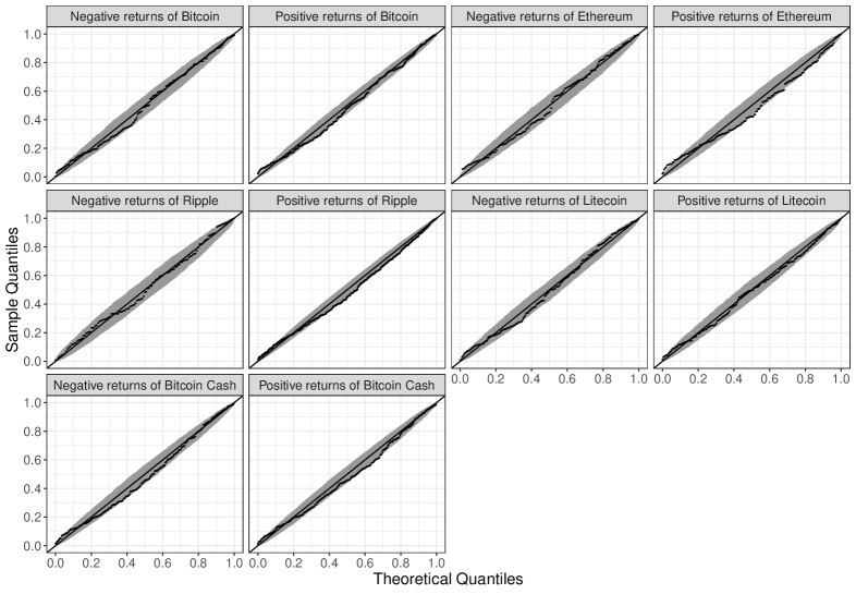
Finally, we evaluate the goodness of fit of the model using the similar method appeared in Wang and Tsai (2009). From (9), the distribution of Sijexp[γ(Uj,𝑿ij)1S_{ij}\coloneqq\exp[-\gamma(U_{j},{\bm{X}}_{ij})^{-1}
log(Yij/ωj)]\log(Y_{ij}/\omega_{j})] conditional on Uj,𝑿ijU_{j},{\bm{X}}_{ij} and Yij>ωjY_{ij}>\omega_{j} can be approximated by the uniform distribution on [0,1][0,1] (see, Wang and Tsai 2009). Let S~ij\tilde{S}_{ij} be SijS_{ij} with θA=θ^A\theta_{\rm{A}}=\hat{\theta}_{\rm{A}}, 𝜽B=𝜽^B{\bm{\theta}}_{\rm{B}}=\hat{\bm{\theta}}_{\rm{B}} and Uj=u~jU_{j}=\tilde{u}_{j}. Then, for each j=1,2,,413j=1,2,\ldots,413, 𝒮j{S~ij:Yij>ωj,i=1,2,,nj}\mathcal{S}_{j}\coloneqq\{\tilde{S}_{ij}:Y_{ij}>\omega_{j},\ i=1,2,\ldots,n_{j}\} can be considered as a uniformly distributed random sample. Figure 1 shows the Q-Q plots of 𝒮j\mathcal{S}_{j} against equally divided points on [0,1][0,1] for the five representative cryptocurrencies discussed above, where the bands are the 95% pointwise confidence bands constructed by the function geom_qq_band() with bandType="boot" in the package qqplotr (see, Almeida, Loy, and Hofmann 2018) within R. In each panel of Figure 1, the points were approximately aligned on a straight line with an intercept of 0 and slope of 1. This means that our model fits both negative and positive returns well for each of the five stocks.

Refer to caption
Figure 1: The Q-Q plots for Bitcoin, Ethereum, Ripple, Litecoin and Bitcoin Cash.

4.4 Comparison

In this section, we compare our model (14) with the method proposed by Wang and Tsai (2009). The latter competitor applies the EVI regression to data stock by stock. To compare these two methods, we iteratively compute the following 2-fold cross-validation criterion. At each iteration step, the returns for each stock are randomly divided into training and test data. As a criterion, we adapt the discrepancy measure proposed by Wang and Tsai (2009). For each of our model and the model of Wang and Tsai (2009), the discrepancy measure for each stock is computed from the test data using the estimated parameters, predicted random effects, and selected thresholds from the training data. Note that our model and the model proposed by Wang and Tsai (2009) use the same threshold exceedances (see, Section 2.4). After 100 iterations, we take the average of the discrepancy measures obtained for each stock. Each panel of Figure 2 shows the scatter plot of averaged discrepancy measures between our model and the model of Wang and Tsai (2009) for the 413 stocks. We can see from the results that the discrepancy measures of our model are smaller than those of Wang and Tsai (2009) for many stocks for both negative and positive returns, suggesting that our model provides better performance.

Refer to caption
Figure 2: The scatter plot of the discrepancy measures between the model proposed by Wang and Tsai (2009) and our model, for the 413 stocks.

5 Discussion

In this study, we investigated the MEM for the EVI in the Pareto-type distribution for unit-level data. In other words, this study incorporated the method of SAE into EVT. As explained in Section 2, the parameters of the proposed model were estimated by the maximum likelihood method, and the random effects were predicted by the conditional mode. In Section 3, we established the asymptotic normality of the estimator. Together with the simulation studies in Section 1 of our supplementary material and real data example in Section 4, we can conclude the following advantages of using the MEM for EVI regression. First, in extreme value analysis, the sample size is generally small for some areas because of the peak over threshold. However, as described in Sections 1.3 of our supplementary material and Section 4, the common parametric part in the MEM can adequately guide the differences between areas. Interestingly, the “borrowing of strength” of the MEM is effective for EVI regression because it improves the bias and variance of the peak-over-threshold method (see, Section 1.3 of our supplementary material). Thus, the proposed model provides a significantly efficient tool that is an alternative to direct estimates from each area. Second, the proposed model is effective even when the number of areas is large. This is shown theoretically in Theorem 1 of Section 3.2, while Section 1.2 of our supplementary material proves this property numerically. Furthermore, as a result supporting the use of the proposed model, in Section 1.3 of our supplementary material, the extreme value analysis using the MEM provided more reasonable results than the fully parametric model. Finally, in extreme value analysis, general EVI estimators sometimes have a large bias resulting from the approximation of the peak over threshold. However, from Theorem 1, we found that when JJ is large, the proposed estimator can be designed to reduce the bias while maintaining its stable variance. This is a somewhat surprising result, because a large number of areas typically leads to poor performance of the estimator in the fully parametric model. Thus, the MEM may be one of the effective approaches to overcome the severe problem of bias in extreme value analysis.

We describe future research using the MEM for extreme value analysis. The first work of interest is the development of models such as the simultaneous autoregressive model and the conditional autoregressive model to explain the dependencies between areas (see, Rao and Molina 2015 and references therein). Such models may help provide better estimates in some applications, including spatial data. Second, it may be feasible to extend the MEM to other EVT models such as the generalized extreme value distribution and GPD. In this study, the methods derived from these models and their theoretical results were not clarified and thus require future detailed study. Third, we expect to extend the MEM to extreme quantile regression (see, Wang, Li, and He 2012; Wang and Li 2013). Finally, although this paper studied the MEM with Gaussian random effects, it may be important to consider other distributions of the random effects (see, Section 9.2 of Wu 2009 and Yavuz and Arslan 2018). The development of the MEM with non-Gaussian random effects is also an interesting future work in EVT.

Acknowledgments

We would like to thank Editage (https://www.editage.jp/) for the English language editing.

Data availability statement

The dataset analyzed during this study was processed from those obtained from CoinMarketCap (see, https://coinmarketcap.com/). This dataset and the associated code of R (https://www.r-project.org/) are available from the corresponding author on reasonable request.

References

  • [1] Almeida, S., A. Loy, and H. Hofmann. 2018. ggplot2 compatible quantile-quantile plots in R. The R Journal 10 (2):248-61. doi:10.32614/RJ-2018-051.
  • [2] Bates, D., M. Mächler, B. Bolker, and S. Walker. 2015. Fitting linear mixed-effects models using lme4. Journal of Statistical Software 67 (1):1-48. doi:10.18637/jss.v067.i01.
  • [3] Battese, G., R. Harter, and W. Fuller. 1988. An error-components model for prediction of county crop areas using survey and satellite data. Journal of the American Statistical Association 83 (401):28-36. doi:10.1080/01621459.1988.10478561.
  • [4] Beirlant, J., and Y. Goegebeur. 2003. Regression with response distributions of Pareto-type. Computational Statistics & Data Analysis 42 (4):595-619. doi:10.1016/S0167-9473(02)00120-2.
  • [5] Beirlant, J., Y. Goegebeur, J. Teugels, and J. Segers. 2004. Statistics of extremes: Theory and applications. New Jersey: John Wiley & Sons.
  • [6] Bottolo, L., G. Consonni, P. Dellaportas, and A. Lijoi. 2003. Bayesian analysis of extreme values by mixture modeling. Extremes 6 (1):25-47. doi:10.1023/A:1026225113154.
  • [7] Broström, G., and H. Holmberg. 2011. Generalized linear models with clustered data: Fixed and random effects models. Computational Statistics & Data Analysis 55 (12):3123-34. doi:10.1016/j.csda.2011.06.011.
  • [8] Davison, A. C., and R. L. Smith. 1990. Models for exceedances over high thresholds. Journal of the Royal Statistical Society: Series B (Methodological) 52 (3):393-425. doi:10.1111/j.2517-6161.1990.tb01796.x.
  • [9] de Carvalho, M., R. Huser, and R. Rubio. 2023. Similarity-based clustering for patterns of extreme values. Stat 12 (1):e560. doi:10.1002/sta4.560.
  • [10] Dempster, A. P., D. B. Rubin, and R. K. Tsutakawa. 1981. Estimation in covariance components models. Journal of the American Statistical Association 76 (374):341-53. doi:10.1080/01621459.1981.10477653.
  • [11] Diallo, M., and J. N. K. Rao. 2018. Small area estimation of complex parameters under unit-level models with skew-normal errors. Scandinavian Journal of Statistics 45 (4):1092-116. doi:10.1111/sjos.12336.
  • [12] Dupuis, D. J., S. Engelke, and L. Trapin. 2023. Modeling panels of extremes. The Annals of Applied Statistics 17 (1):498-517. doi:10.1214/22-AOAS1639.
  • [13] Fisher, R., and L. Tippett. 1928. Limiting forms of the frequency distribution of the largest or smallest member of a sample. Mathematical Proceedings of the Cambridge Philosophical Society 24 (2):180-90. doi:10.1017/S0305004100015681.
  • [14] Gkillas, K., and P. Katsiampa. 2018. An application of extreme value theory to cryptocurrencies. Economics Letters 164:109-11. doi:10.1016/j.econlet.2018.01.020.
  • [15] Gumbel, E. J. 1958. Statistics of extremes. West Sussex: Columbia University Press.
  • [16] Hall, P. 1982. On some simple estimates of an exponent of regular variation. Journal of the Royal Statistical Society: Series B (Methodological) 44 (1):37-42. doi:10.1111/j.2517-6161.1982.tb01183.x.
  • [17] Hill, B. M. 1975. A simple general approach to inference about the tail of a distribution. The Annals of Statistics 3 (5):1163-74. doi:10.1214/aos/1176343247.
  • [18] Jiang, J. 2007. Linear and generalized linear mixed models and their applications. New York: Springer.
  • [19] Jiang, J. 2017. Asymptotic analysis of mixed effects models: Theory, applications, and open problems. Boca Raton, Florida: CRC Press.
  • [20] Jiang, J., M. P. Wand, and A. Bhaskaran. 2022. Usable and precise asymptotics for generalized linear mixed model analysis and design. Journal of the Royal Statistical Society: Series B (Statistical Methodology) 84 (1):55-82. doi:10.1111/rssb.12473.
  • [21] Longin, F., and G. Pagliardi. 2016. Tail relation between return and volume in the US stock market: An analysis based on extreme value theory. Economics Letters 145:252-4. doi:10.1016/j.econlet.2016.06.026.
  • [22] Ma, Y., Y. Jiang, and W. Huang. 2019. Tail index varying coefficient model. Communications in Statistics - Theory and Methods 48 (2):235-56. doi:10.1080/03610926.2017.1406519.
  • [23] Magnus, J. R., and H. Neudecker. 1988. Matrix differential calculus with applications in statistics and econometrics. New Jersey: John Wiley & Sons.
  • [24] Molina, I., P. Corral, and M. Nguyen. 2022. Estimation of poverty and inequality in small areas: Review and discussion. TEST 31 (4):1143-66. doi:10.1007/s11749-022-00822-1.
  • [25] Molina, I., and J. N. K. Rao. 2010. Small area estimation of poverty indicators. The Canadian Journal of Statistics 38 (3):369-85. https://www.jstor.org/stable/27896031.
  • [26] Nie, L. 2007. Convergence rate of MLE in generalized linear and nonlinear mixed-effects models: Theory and applications. Journal of Statistical Planning and Inference 137 (6):1787-804. doi:10.1016/j.jspi.2005.06.010.
  • [27] R Core Team. 2021. R: A Language and Environment for Statistical Computing. Vienna, Austria: R Foundation for Statistical Computing.
  • [28] Rao, J. N. K., and I. Molina. 2015. Small area estimation. Hoboken, New Jersey: John Wiley & Sons.
  • [29] Reiss, R. D., and M. Thomas. 2007. Statistical analysis of extreme values: With applications to insurance, finance, hydrology and other fields. Basel, Switzerland: Birkhäuser Basel.
  • [30] Rohrbeck, C., and J. Tawn. 2021. Bayesian spatial clustering of extremal behavior for hydrological variables. Journal of Computational and Graphical Statistics 30 (1):91-105. doi:10.1080/10618600.2020.1777139.
  • [31] Ruppert, D., M. P. Wand, and R. J. Carroll. 2003. Semiparametric regression. New York: Cambridge University Press.
  • [32] Santner, T. J., and D. E. Duffy. 1989. The statistical analysis of discrete data. New York: Springer.
  • [33] Sugasawa, S., and T. Kubokawa. 2020. Small area estimation with mixed models: A review. Japanese Journal of Statistics and Data Science 3 (2):693-720. doi:10.1007/s42081-020-00076-x.
  • [34] Torabi, M. 2019. Spatial generalized linear mixed models in small area estimation. Canadian Journal of Statistics 47 (3):426-37. doi:10.1002/cjs.11502.
  • [35] Wang, H. J., and D. Li. 2013. Estimation of extreme conditional quantiles through power transformation. Journal of the American Statistical Association 108 (503):1062-74. doi:10.1080/01621459.2013.820134.
  • [36] Wang, H. J., D. Li, and X. He. 2012. Estimation of high conditional quantiles for heavy-tailed distributions. Journal of the American Statistical Association 107 (500):1453-64. doi:10.1080/01621459.2012.716382.
  • [37] Wang, H., and C. L. Tsai. 2009. Tail index regression. Journal of the American Statistical Association 104 (487):1233-40. doi:10.1198/jasa.2009.tm08458.
  • [38] Wu, L. 2009. Mixed effects models for complex data. Boca Raton, Florida: CRC Press.
  • [39] Yavuz, F. G., and O. Arslan. 2018. Linear mixed model with Laplace distribution (LLMM). Statistical Papers 59 (1):271-289. doi:10.1007/s00362-016-0763-x.

Supplemental online material for
“Mixed effects models for extreme value index regression”


This supplementary material supports our main article entitled “Mixed effects models for extreme value index regression” and is organized as follows. Section 1 provides some Monte Carlo simulation studies to verify the finite sample performance of the model proposed in Section 2 of our main article. Section 2 describes the technical details of the proof of Theorem 1 in Section 3.2 of our main article. Note that we use many of the symbols defined in our main article.

1 Simulation

From Eq. (9) of our main article, we can approximate the distribution of log(Yij/ωj)\log(Y_{ij}/\omega_{j}) conditional on 𝑼j{\bm{U}}_{j}, 𝑿ij{\bm{X}}_{ij} and Yij>ωjY_{ij}>\omega_{j} by the exponential distribution, which belongs to the gamma distribution (see, Wang and Tsai 2009). Therefore, our estimator (𝜽^A,𝜽^B,𝚺^)(\hat{\bm{\theta}}_{\rm{A}},\hat{\bm{\theta}}_{\rm{B}},\hat{\bm{\Sigma}}) and predictor 𝒖~j\tilde{\bm{u}}_{j} proposed in Section 2 of our main article can be easily implemented by using the function glmer() with family=Gamma(link="log") in the package lme4 (see, Bates et al. 2015) within the R computing environment (see, R Core Team 2021). In the function glmer(), when pA=1p_{\rm{A}}=1, the integral in the log-likelihood defined in Eq. (10) of our main article is approximated by the adaptive Gauss-Hermite quadrature, and 𝚺^\hat{\bm{\Sigma}} and (𝜽^A,𝜽^B)(\hat{\bm{\theta}}_{\rm{A}},\hat{\bm{\theta}}_{\rm{B}}) are then optimized by “bobyqa” and “Nelder Mead”, respectively.

In the following Sections 1.1-1.3, we investigate the performance of our estimator (𝜽^A,𝜽^B,𝚺^)(\hat{\bm{\theta}}_{\rm{A}},\hat{\bm{\theta}}_{\rm{B}},\hat{\bm{\Sigma}}) and predictor 𝒖~j\tilde{\bm{u}}_{j} through some simulation studies using the above package.

1.1 Practicality of asymptotic normality of the estimator

In this section, we illustrate the applicability of our asymptotic normality constructed in Corollary 1 of our main article to finite samples. This is positioned as a preliminary study for hypothesis testing on a real data example in Section 4 of our main article.

We simulate the dataset {(Yij,𝑿ij)}i𝒩j,j𝒥\{(Y_{ij},{\bm{X}}_{ij})\}_{i\in\mathcal{N}_{j},j\in\mathcal{J}} as follows. Let denote 𝑿ij=(Xij(1),Xij(2))2{\bm{X}}_{ij}=(X_{ij}^{(1)},X_{ij}^{(2)})^{\top}\in\mathbb{R}^{2} and set Xij(1)1X_{ij}^{(1)}\equiv 1 for i𝒩ji\in\mathcal{N}_{j} and j𝒥j\in\mathcal{J}. First, we independently generate {Xij(2)}i𝒩j,j𝒥\{X_{ij}^{(2)}\}_{i\in\mathcal{N}_{j},j\in\mathcal{J}} from the standard normal distribution or uniform distribution on [3,3][-\sqrt{3},\sqrt{3}]. Note that in both covariate cases, Xij(2)X_{ij}^{(2)} has zero mean and unit variance. In the next step, we obtain an independent sample {Uj}j𝒥\{U_{j}\}_{j\in\mathcal{J}} from N(0,σ2)N(0,\sigma^{2}) with σ2=0.2\sigma^{2}=0.2. Finally, for each i𝒩ji\in\mathcal{N}_{j} and j𝒥j\in\mathcal{J}, we generate YijY_{ij} using a given conditional response distribution F(Uj,Xij(2))F(\cdot\mid U_{j},X_{ij}^{(2)}). The same data generation procedure will be used in Section 1.2. Here, to obtain {Yij}i𝒩j,j𝒥\{Y_{ij}\}_{i\in\mathcal{N}_{j},j\in\mathcal{J}}, we use the Pareto distribution

F(yUj,Xij(2))=1y1/γ(Uj,Xij(2))F(y\mid U_{j},X_{ij}^{(2)})=1-y^{-1/\gamma(U_{j},X_{ij}^{(2)})} (16)

and apply the nested error regression type model formulated as Eq. (7) of our main article with 𝑿Aij=Xij(1){\bm{X}}_{{\rm{A}}ij}=X_{ij}^{(1)} and 𝑿Bij=Xij(2){\bm{X}}_{{\rm{B}}ij}=X_{ij}^{(2)}, i.e.,

γ(Uj,Xij(2))=exp(θA(1)+Uj+θB(2)Xij(2)),\gamma(U_{j},X_{ij}^{(2)})=\exp\left(\theta_{\rm{A}}^{(1)}+U_{j}+\theta_{\rm{B}}^{(2)}X_{ij}^{(2)}\right), (17)

where (θA(1),θB(2))=(0.5,0.2)(\theta_{\rm{A}}^{(1)},\theta_{\rm{B}}^{(2)})=(-0.5,0.2). Let us denote the proposed estimator of (θA(1),θB(2),σ2)(\theta_{\rm{A}}^{(1)},\theta_{\rm{B}}^{(2)},\sigma^{2}) by (θ^A(1),θ^B(2),σ^2)(\hat{\theta}_{\rm{A}}^{(1)},\hat{\theta}_{\rm{B}}^{(2)},\hat{\sigma}^{2}). Because the Pareto distribution (16) satisfies Eq. (12) of our main article with β(Uj,Xij(2))=\beta(U_{j},X_{ij}^{(2)})=\infty, the estimator does not have the asymptotic bias described in Remark 1 in Section 3.2 of our main article. Therefore, we do not use the thresholds ωj,j𝒥\omega_{j},\ j\in\mathcal{J}, and thus the effective sample size nj0n_{j0} for each j𝒥j\in\mathcal{J} is unchanged from njn_{j}.

Refer to caption
Figure 3: Results of the simulation with the normal covariate: Q-Q plots for the standardized estimates against N(0,1)N(0,1).
Refer to caption
Figure 4: Results of the simulation with the uniform covariate: Q-Q plots for the standardized estimates against N(0,1)N(0,1).

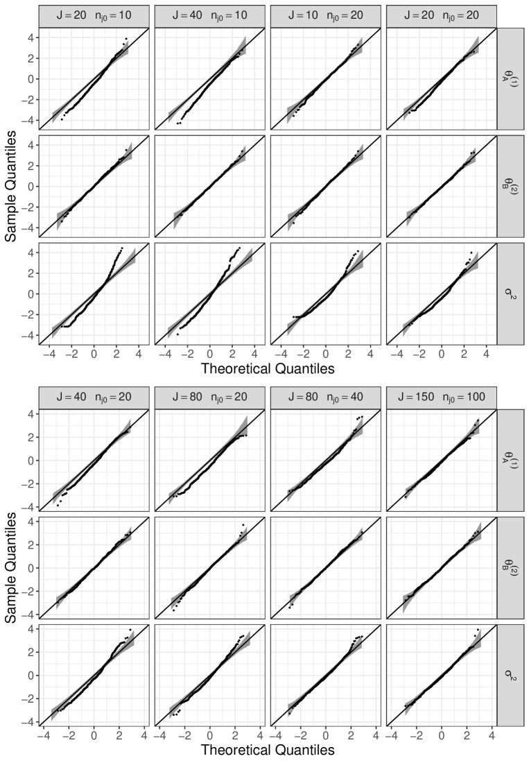
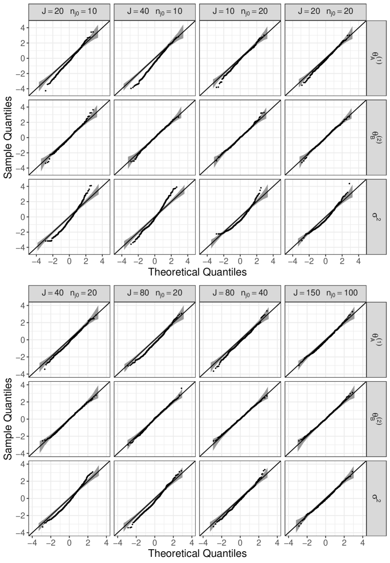
Under the above model setups, from Corollary 1 of our main article, J1/2(θ^A(1)θA(1))/σJ^{1/2}(\hat{\theta}_{\rm{A}}^{(1)}-\theta_{\rm{A}}^{(1)})/\sigma, (Jn0)1/2(θ^B(2)θB(2))(Jn_{0})^{1/2}(\hat{\theta}_{\rm{B}}^{(2)}-\theta_{\rm{B}}^{(2)}) and J1/2(σ^2σ2)/(2σ2)J^{1/2}(\hat{\sigma}^{2}-\sigma^{2})/(\sqrt{2}\sigma^{2}) are asymptotically distributed as N(0,1)N(0,1). Note that this simulation setting satisfies 𝛀B=1{\bm{\Omega}}_{\rm{B}}=1 in Corollary 1 of our main article. To obtain the empirical distributions of the above standardized estimators, we use 500 datasets and repeatedly estimate the parameters {θA(1),θB(2),σ2}\{\theta_{\rm{A}}^{(1)},\theta_{\rm{B}}^{(2)},\sigma^{2}\} from each dataset. Figures 3 and 4 show the Q-Q plots for the obtained standardized estimates against N(0,1)N(0,1) for the normal covariate and uniform covariate, respectively. In these figures, (J,nj0)(J,n_{j0}) varies by column as (20,10)(20,10), (40,10)(40,10), (10,20)(10,20), (20,20)(20,20), (40,20)(40,20), (80,20)(80,20), (80,40)(80,40), and (150,100)(150,100). Furthermore, the bands in each panel are the 95% pointwise confidence bands constructed by the function geom_qq_band() with bandType="boot" in the package qqplotr (see, Almeida, Loy, and Hofmann 2018) within R. If all generated U1,U2,,UJU_{1},U_{2},\ldots,U_{J} are close to each other, σ2\sigma^{2} may be estimated to be zero by glmer(). Thus, for J=10J=10 and J=20J=20, the Q-Q plot contained several equal values for σ2\sigma^{2}. Comparing Figures 3 and 4, the type of the distribution of Xij(2){X}_{ij}^{(2)} did not significantly affect the results. We can see from Figures 3 and 4 that for θA(1)\theta_{\rm{A}}^{(1)} and σ2\sigma^{2}, the empirical distribution of the standardized estimators had heavier tails than N(0,1)N(0,1), but this tendency disappeared with increasing JJ and nj0n_{j0}. In contrast to θA(1)\theta_{\rm{A}}^{(1)} and σ2\sigma^{2}, the Q-Q plot for θB(2)\theta_{\rm{B}}^{(2)} was good for all pairs of (J,nj0)(J,n_{j0}). Consequently, these results reflect the claims of Corollary 1 of our main article.

1.2 Behavior of the estimator for numerous areas

In this section, we examine the numerical performance of the estimator for large JJ. To obtain the dataset {(Yij,𝑿ij)}i𝒩j,j𝒥\{(Y_{ij},{\bm{X}}_{ij})\}_{i\in\mathcal{N}_{j},j\in\mathcal{J}} according to the procedure in Section 1.1, we use (17) and the following conditional distribution (a) or (b) instead of (16):

  1. (a)

    Student’s tt-distribution

    F(yUj,Xij(2))\displaystyle F(y\mid U_{j},X_{ij}^{(2)})
    =yΓ([ν(Uj,Xij(2))+1]/2)ν(Uj,Xij(2))πΓ(ν(Uj,Xij(2))/2)[1+t2ν(Uj,Xij(2))][ν(Uj,Xij(2))+1]/2𝑑t\displaystyle=\int_{-\infty}^{y}\frac{\Gamma([\nu(U_{j},X_{ij}^{(2)})+1]/2)}{\sqrt{\nu(U_{j},X_{ij}^{(2)})\pi}\Gamma(\nu(U_{j},X_{ij}^{(2)})/2)}\left[1+\frac{t^{2}}{\nu(U_{j},X_{ij}^{(2)})}\right]^{-\left[\nu(U_{j},X_{ij}^{(2)})+1\right]/2}dt

    with ν(Uj,Xij(2))γ(Uj,Xij(2))1\nu(U_{j},X_{ij}^{(2)})\coloneqq\gamma(U_{j},X_{ij}^{(2)})^{-1}, where Γ()\Gamma(\cdot) is a gamma function. For Eq. (12) of our main article, this distribution belongs to the Pareto-type distribution with β(Uj,Xij(2))2\beta(U_{j},X_{ij}^{(2)})\equiv 2.

  2. (b)

    Burr distribution

    F(yUj,Xij(2))=1[ηη+yτ(Uj,Xij(2))]κF(y\mid U_{j},X_{ij}^{(2)})=1-\left[\frac{\eta}{\eta+y^{\tau(U_{j},X_{ij}^{(2)})}}\right]^{\kappa}

    with η=1\eta=1, κ=1\kappa=1 and τ(Uj,Xij(2))γ(Uj,Xij(2))1\tau(U_{j},X_{ij}^{(2)})\coloneqq\gamma(U_{j},X_{ij}^{(2)})^{-1}. The Burr distribution satisfies Eq. (12) of our main article with β(Uj,Xij(2))=τ(Uj,Xij(2))\beta(U_{j},X_{ij}^{(2)})=\tau(U_{j},X_{ij}^{(2)}).

For (a), we obtain a sample directly from the tt-distribution for a given non-integer degree of freedom. As described in Remark 1 of our main article, the proposed estimator is more biased for smaller β(Uj,Xij(2))\beta(U_{j},X_{ij}^{(2)}).

Refer to caption
Figure 5: Simulation results for the distribution (a) with the normal covariate: Variations of the sample squared bias (×103)(\times 10^{3}) and variance (×103)(\times 10^{3}) of the estimator with respect to JJ and TT.
Refer to caption
Figure 6: Simulation results for the distribution (a) with the uniform covariate: Variations of the sample squared bias (×103)(\times 10^{3}) and variance (×103)(\times 10^{3}) of the estimator with respect to JJ and TT.
Refer to caption
Figure 7: Simulation results for the distribution (b) with the normal covariate: Variations of the sample squared bias (×103)(\times 10^{3}) and variance (×103)(\times 10^{3}) of the estimator with respect to JJ and TT.
Refer to caption
Figure 8: Simulation results for the distribution (b) with the uniform covariate: Variations of the sample squared bias (×103)(\times 10^{3}) and variance (×103)(\times 10^{3}) of the estimator with respect to JJ and TT.

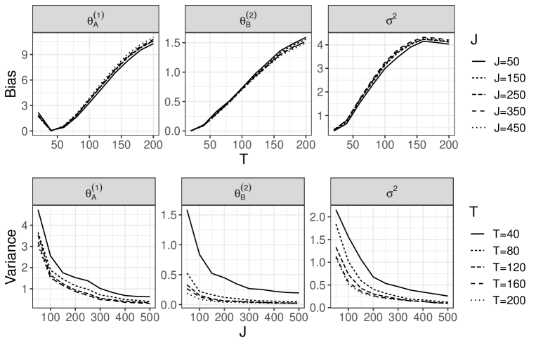
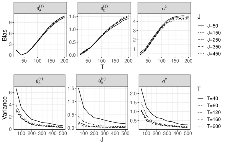
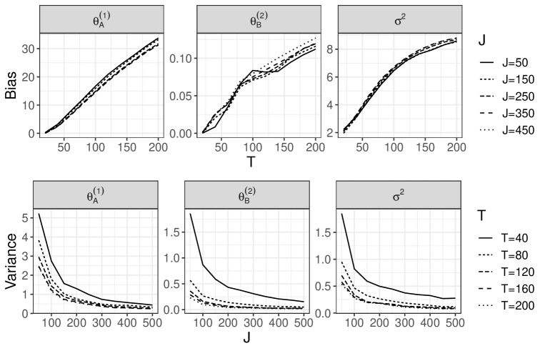
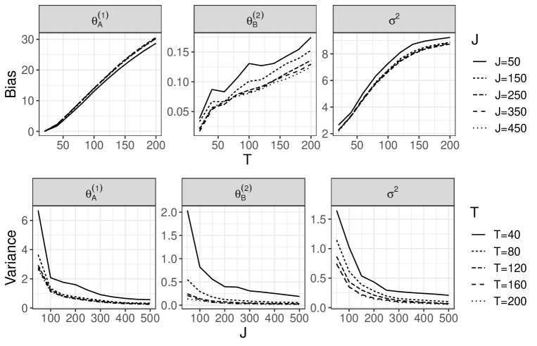
In advance, we generate the unit-level data with 500 areas and nj=1000n_{j}=1000 using the above procedure. Then, we use a part of the dataset according to the following rules. The number of areas JJ is increased by a factor of 10 from 50 to 500. Furthermore, for the discrepancy measure described in Section 2.4 of our main article, we use the 10th to TTth largest responses in the jjth area as the candidates for the jjth threshold ωj\omega_{j}, where TT varies from 20 to 200 in increments of 20. Roughly speaking, a smaller TT means that higher thresholds ωj,j𝒥\omega_{j},\ j\in\mathcal{J} are chosen. For each JJ and TT, we obtain the estimates {θ^A(1),θ^B(2),σ^2}\{\hat{\theta}_{\rm{A}}^{(1)},\hat{\theta}_{\rm{B}}^{(2)},\hat{\sigma}^{2}\}. Following the above rules, we iterate the estimation for 100 sets of unit-level data. Figures 5-8 show the sample squared bias and variance of the estimator for each JJ and TT. The details can be found in the description of each figure. Overall, we can see that our estimator remained stable when JJ was sufficiently large, even when TT was small. Based on the first row of each figure, our estimator then did not suffer from a large bias for large JJ. Such results guarantee the considerations in Remark 2 of Section 3.2 of our main article. As described in Remark 1 of our main article, from the second row of each figure, the variance of θ^B(2)\hat{\theta}_{\rm{B}}^{(2)} was strongly dependent on both JJ and TT when JJ was small, while the variances of θ^A(1)\hat{\theta}_{\rm{A}}^{(1)} and σ^2\hat{\sigma}^{2} were almost unaffected by TT.

1.3 Borrowing of strength for extremes

In this section, we compare our model, the fully parametric model defined in Eqs. (2) and (3) of our main article, and model proposed by Wang and Tsai (2009). The use of the model proposed by Wang and Tsai (2009) implies that areas are analyzed separately. To obtain the estimates for the latter two parametric models, we use the function glm() with family=Gamma(link="log") within R.

Unlike Sections 1.1 and 1.2, the dataset {(Yij,𝑿ij)}i𝒩j,j𝒥\{(Y_{ij},{\bm{X}}_{ij})\}_{i\in\mathcal{N}_{j},j\in\mathcal{J}} is simulated from the fully parametric model as follows. Let JJ be divided into J=J+JJ=J^{\dagger}+J^{\ddagger} and set J=130J^{\dagger}=130, J=20J^{\ddagger}=20, n1==nJ=100n_{1}=\cdots=n_{J^{\dagger}}=100 and nJ+1==nJ+J=20n_{J^{\dagger}+1}=\cdots=n_{J^{\dagger}+J^{\ddagger}}=20. We generate {Xij(2)}i𝒩j,j𝒥\{X_{ij}^{(2)}\}_{i\in\mathcal{N}_{j},j\in\mathcal{J}} from N(0,1)N(0,1). To generate {Yij}i𝒩j,j𝒥\{Y_{ij}\}_{i\in\mathcal{N}_{j},j\in\mathcal{J}}, we then combine the two distributions

Fj(yXij(2))=1y1/γj(Xij(2)),j=1,2,,JF_{j}^{\dagger}(y\mid X_{ij}^{(2)})=1-y^{-1/\gamma_{j}(X_{ij}^{(2)})},\quad j=1,2,\ldots,J^{\dagger} (18)

and

Fj(yXij(2))=11.5y1/γj(Xij(2))1+0.5y1/γj(Xij(2)),j=J+1,J+2,,J+J,F_{j}^{\ddagger}(y\mid X_{ij}^{(2)})=1-\frac{1.5y^{-1/\gamma_{j}(X_{ij}^{(2)})}}{1+0.5y^{-1/\gamma_{j}(X_{ij}^{(2)})}},\quad j=J^{\dagger}+1,J^{\dagger}+2,\ldots,J^{\dagger}+J^{\ddagger}, (19)

where FjF_{j}^{\ddagger} is described in detail in Section 4.1 of Wang and Tsai (2009). Then, the extreme value index γj(Xij(2))\gamma_{j}(X_{ij}^{(2)}) is modeled as γj(Xij(2))=exp(θjA(1)+θB(2)Xij(2))\gamma_{j}(X_{ij}^{(2)})=\exp(\theta_{j{\rm{A}}}^{(1)}+\theta_{\rm{B}}^{(2)}X_{ij}^{(2)}), where θB(2)=0.2\theta_{\rm{B}}^{(2)}=0.2 and the parameters θjA(1),j𝒥\theta_{j{\rm{A}}}^{(1)},\ j\in\mathcal{J} are assigned the following two types. One θjA(1)\theta_{j{\rm{A}}}^{(1)} is defined as the j/(J+1)j/(J^{\dagger}+1)-th quantile of N(0,1/12)N(0,1/12) for j=1,2,,Jj=1,2,\ldots,J^{\dagger} and (jJ)/(J+1)(j-J^{\dagger})/(J^{\ddagger}+1)-th quantile of N(0,1/12)N(0,1/12) for j=J+1,J+2,,J+Jj=J^{\dagger}+1,J^{\dagger}+2,\ldots,J^{\dagger}+J^{\ddagger}, and the other θjA(1)\theta_{j{\rm{A}}}^{(1)} is fixed as 0.5+0.5(j1)/(J1)-0.5+0.5(j-1)/(J^{\dagger}-1) for j=1,2,,Jj=1,2,\ldots,J^{\dagger} and 0.5+0.5(jJ1)/(J1)-0.5+0.5(j-J^{\dagger}-1)/(J^{\ddagger}-1) for j=J+1,J+2,,J+Jj=J^{\dagger}+1,J^{\dagger}+2,\ldots,J^{\dagger}+J^{\ddagger}. These two settings of θjA(1)\theta_{j{\rm{A}}}^{(1)} are denoted by Normal type and Uniform type, respectively.

Table 3: Sample bias and variance of the estimator for the three models.
Our model Fully parametric model Direct estimates
Normal type
θjA(1)\theta_{j{\rm{A}}}^{(1)} Bias\text{Bias}^{\dagger} 1.77×10³-1.77\times 10^{-3} 4.39×10³-4.39\times 10^{-3} 9.50×10³-9.50\times 10^{-3}
Bias\text{Bias}^{\ddagger} 1.20×1011.20\times 10^{-1} 1.77×1011.77\times 10^{-1} 1.57×1011.57\times 10^{-1}
Variance\text{Variance}^{\dagger} 7.89×1037.89\times 10^{-3} 9.97×1039.97\times 10^{-3} 1.01×1021.01\times 10^{-2}
Variance\text{Variance}^{\ddagger} 1.69×1021.69\times 10^{-2} 4.25×1024.25\times 10^{-2} 4.59×1024.59\times 10^{-2}
θB(2)\theta_{\rm{B}}^{(2)} Bias 2.00×1012.00\times 10^{-1} 2.00×1012.00\times 10^{-1} 2.00×1012.00\times 10^{-1}
Variance 6.78×1056.78\times 10^{-5} 6.78×1056.78\times 10^{-5} 1.23×1041.23\times 10^{-4}
Uniform type
θjA(1)\theta_{j{\rm{A}}}^{(1)} Bias\text{Bias}^{\dagger} 3.07×10³-3.07\times 10^{-3} 5.56×10³-5.56\times 10^{-3} 1.06×10²-1.06\times 10^{-2}
Bias\text{Bias}^{\ddagger} 1.26×1011.26\times 10^{-1} 1.80×1011.80\times 10^{-1} 1.60×1011.60\times 10^{-1}
Variance\text{Variance}^{\dagger} 8.07×1038.07\times 10^{-3} 9.98×1039.98\times 10^{-3} 1.01×1021.01\times 10^{-2}
Variance\text{Variance}^{\ddagger} 1.73×1021.73\times 10^{-2} 4.10×1024.10\times 10^{-2} 4.50×1024.50\times 10^{-2}
θB(2)\theta_{\rm{B}}^{(2)} Bias 2.00×1012.00\times 10^{-1} 2.00×1012.00\times 10^{-1} 1.99×1011.99\times 10^{-1}
Variance 7.32×1057.32\times 10^{-5} 7.34×1057.34\times 10^{-5} 1.13×1041.13\times 10^{-4}

Without introducing thresholds, we estimate θjA(1),j𝒥\theta_{j{\rm{A}}}^{(1)},\ j\in\mathcal{J} and θB(2)\theta_{\rm{B}}^{(2)} by each of our model, the fully parametric model expressed as Eqs. (2) and (3) of our main article, and model proposed by Wang and Tsai (2009). In our model, estimates for θAj(1),j𝒥\theta_{{\rm{A}}j}^{(1)},\ j\in\mathcal{J} are obtained by combining the estimator and predictor proposed in Section 2 of our main article. For the model proposed by Wang and Tsai (2009), different estimates of θB(2)\theta_{\rm{B}}^{(2)} are obtained across the areas, but the mean of these is used as the estimate of θB(2)\theta_{\rm{B}}^{(2)}. Under the above simulation settings, if the areas were analyzed separately, the estimates for the areas from (19) would have large bias and variance. Therefore, we are interested in whether these direct estimates can be improved by simultaneously analyzing the areas using our model. To verify this, we evaluate the sample bias and variance of the estimator for each method. Table 3 shows the results based on 500 sets of unit-level data, where the superscripts {\dagger} and {\ddagger} in this table refer to the means for j=1,2,,Jj=1,2,\ldots,J^{\dagger} and for j=J+1,J+2,,J+Jj=J^{\dagger}+1,J^{\dagger}+2,\ldots,J^{\dagger}+J^{\ddagger}, respectively. According to Table 3, our model produced the most stable estimates of the three models. In particular, for θjA(1),j=J+1,J+2,,J+J\theta_{j{\rm{A}}}^{(1)},\ j=J^{\dagger}+1,J^{\dagger}+2,\ldots,J^{\dagger}+J^{\ddagger}, the variance of the estimates was dramatically improved using our model rather than the direct estimates. In addition, we can see that in extreme value analysis, the “borrowing of strength” of the mixed effects model also contributes to reducing the bias of the estimator. In the fully parametric model, the bias of the estimator was larger than that of the direct estimates. Meanwhile, even when the assumption of normality of the random effects in Eq. (4) of our main article was not satisfied, our model was still favorable.

2 Proof of theorems

We give the proof of Theorem 1 in Section 3.2 of our main article. For convenience, we introduce some new symbols:

  • 𝜽Cvech(𝚺){\bm{\theta}}_{\rm{C}}\coloneqq{\rm{vech}}({\bm{\Sigma}}), 𝜽C0vech(𝚺0){\bm{\theta}}_{\rm{C}}^{0}\coloneqq{\rm{vech}}({\bm{\Sigma}}_{0}) and 𝜽^Cvech(𝚺^)\hat{\bm{\theta}}_{\rm{C}}\coloneqq{\rm{vech}}(\hat{\bm{\Sigma}}), which are pCpA(pA+1)/2p_{\rm{C}}\coloneqq p_{\rm{A}}(p_{\rm{A}}+1)/2-dimensional vectors.

  • 𝜽(𝜽A,𝜽B,𝜽C){\bm{\theta}}\coloneqq({\bm{\theta}}_{\rm{A}}^{\top},{\bm{\theta}}_{\rm{B}}^{\top},{\bm{\theta}}_{\rm{C}}^{\top})^{\top}, 𝜽0((𝜽A0),(𝜽B0),(𝜽C0)){\bm{\theta}}^{0}\coloneqq(({\bm{\theta}}_{\rm{A}}^{0})^{\top},({\bm{\theta}}_{\rm{B}}^{0})^{\top},({\bm{\theta}}_{\rm{C}}^{0})^{\top})^{\top} and 𝜽^(𝜽^A,𝜽^B,𝜽^C)\hat{\bm{\theta}}\coloneqq(\hat{\bm{\theta}}_{\rm{A}}^{\top},\hat{\bm{\theta}}_{\rm{B}}^{\top},\hat{\bm{\theta}}_{\rm{C}}^{\top})^{\top}.

  • For each j𝒥j\in\mathcal{J}, we denote

    j(𝜽)\displaystyle\ell_{j}({\bm{\theta}}) logpAϕ(𝒖;𝟎,𝜽C)exp(i=1nj{(𝜽A+𝒖)𝑿Aij𝜽B𝑿Bij.\displaystyle\coloneqq\log\int_{\mathbb{R}^{p_{\rm{A}}}}\phi({\bm{u}};{\bm{0}},{\bm{\theta}}_{\rm{C}})\exp\left(\sum_{i=1}^{n_{j}}\biggl{\{}-\left({\bm{\theta}}_{\rm{A}}+{\bm{u}}\right)^{\top}{\bm{X}}_{{\rm{A}}ij}-{\bm{\theta}}_{\rm{B}}^{\top}{\bm{X}}_{{\rm{B}}ij}\biggr{.}\right.
    .exp[(𝜽A+𝒖)𝑿Aij𝜽B𝑿Bij]logYijω(J,nj)}I(Yij>ω(J,nj)))d𝒖,\displaystyle\quad\Biggl{.}\left.-\exp\left[-\left({\bm{\theta}}_{\rm{A}}+{\bm{u}}\right)^{\top}{\bm{X}}_{{\rm{A}}ij}-{\bm{\theta}}_{\rm{B}}^{\top}{\bm{X}}_{{\rm{B}}ij}\right]\log\frac{Y_{ij}}{\omega_{(J,n_{j})}}\right\}I(Y_{ij}>\omega_{(J,n_{j})})\Biggr{)}d{\bm{u}},

    where ϕ(𝒖;𝟎,𝜽C)ϕ(𝒖;𝟎,𝚺)\phi({\bm{u}};{\bm{0}},{\bm{\theta}}_{\rm{C}})\coloneqq\phi({\bm{u}};{\bm{0}},{\bm{\Sigma}}). In Eq. (10) of our main article, the approximated log-likelihood (𝜽A,𝜽B,𝚺)\ell({\bm{\theta}}_{\rm{A}},{\bm{\theta}}_{\rm{B}},{\bm{\Sigma}}) can be redefined as (𝜽)j=1Jj(𝜽)\ell({\bm{\theta}})\coloneqq\sum_{j=1}^{J}\ell_{j}({\bm{\theta}}).

  • For any smooth function R1:d;𝒛R1(𝒛)R_{1}:\mathbb{R}^{d}\to\mathbb{R};{\bm{z}}\mapsto R_{1}({\bm{z}}), we denote R1(𝒛)(/𝒛)R1(𝒛)d\nabla R_{1}({\bm{z}})\coloneqq(\partial/\partial{\bm{z}})R_{1}({\bm{z}})\in\mathbb{R}^{d} and 2R1(𝒛)(2/𝒛𝒛)R1(𝒛)d×d\nabla^{2}R_{1}({\bm{z}})\coloneqq(\partial^{2}/\partial{\bm{z}}\partial{\bm{z}}^{\top})R_{1}({\bm{z}})\in\mathbb{R}^{d\times d}. In particular, we denote 𝒛0R1(𝒛)(/𝒛0)R1(𝒛)\nabla_{{\bm{z}}_{0}}R_{1}({\bm{z}})\coloneqq(\partial/\partial{\bm{z}}_{0})R_{1}({\bm{z}}) and 𝒛1𝒛22R1(𝒛)(2/𝒛1𝒛2)R1(𝒛)\nabla_{{\bm{z}}_{1}{\bm{z}}_{2}}^{2}R_{1}({\bm{z}})\coloneqq(\partial^{2}/\partial{\bm{z}}_{1}\partial{\bm{z}}_{2}^{\top})R_{1}({\bm{z}}), where 𝒛0{\bm{z}}_{0}, 𝒛1{\bm{z}}_{1} and 𝒛2{\bm{z}}_{2} are part of 𝒛{\bm{z}}. As a special case, for any smooth real-valued function R2(𝜽)R_{2}({\bm{\theta}}) of 𝜽=(𝜽A,𝜽B,𝜽C){\bm{\theta}}=({\bm{\theta}}_{\rm{A}}^{\top},{\bm{\theta}}_{\rm{B}}^{\top},{\bm{\theta}}_{\rm{C}}^{\top})^{\top}, we simply write KR2(𝜽)𝜽KR2(𝜽)\nabla_{\rm{K}}R_{2}({\bm{\theta}})\coloneqq\nabla_{{\bm{\theta}}_{\rm{K}}}R_{2}({\bm{\theta}}) and K1K22R2(𝜽)𝜽K1𝜽K22R2(𝜽)\nabla_{{\rm{K}}_{1}{\rm{K}}_{2}}^{2}R_{2}({\bm{\theta}})\coloneqq\nabla_{{\bm{\theta}}_{{\rm{K}}_{1}}{\bm{\theta}}_{{\rm{K}}_{2}}}^{2}R_{2}({\bm{\theta}}) for K,K1,K2{A,B,C}{\rm{K}},{\rm{K}}_{1},{\rm{K}}_{2}\in\{{\rm{A}},{\rm{B}},{\rm{C}}\}.

  • For any column vector 𝒛{\bm{z}}, we denote 𝒛2𝒛𝒛{\bm{z}}^{\otimes 2}\coloneqq{\bm{z}}{\bm{z}}^{\top}.

  • Let 𝚼(J,n0){\bm{\Upsilon}}_{(J,n_{0})} be the (pA+pB+pC)(p_{\rm{A}}+p_{\rm{B}}+p_{\rm{C}})-diagonal matrix with diag(𝚼(J,n0))=(J1/2𝟏pA,J1/2n01/2𝟏pB,{\rm{diag}}({\bm{\Upsilon}}_{(J,n_{0})})=(J^{1/2}{\bm{1}}_{p_{\rm{A}}}^{\top},J^{1/2}n_{0}^{1/2}{\bm{1}}_{p_{\rm{B}}}^{\top},
    J1/2𝟏pC)J^{1/2}{\bm{1}}_{p_{\rm{C}}}^{\top})^{\top}, where 𝟏d{\bm{1}}_{d} is the dd-dimensional vector with all elements equal to 1.

Let denote Dj(𝒖)njP(Yij>ω(J,nj)𝑼j=𝒖)/n0D_{j}(\bm{u})\coloneqq n_{j}P(Y_{ij}>\omega_{(J,n_{j})}\mid{\bm{U}}_{j}={\bm{u}})/n_{0}. For each j𝒥j\in\mathcal{J}, Dj(𝒖)D_{j}(\bm{u}) conditional on 𝑼j=𝒖{\bm{U}}_{j}={\bm{u}} satisfies the following Lemma 1.

Lemma 1.

Suppose that (A3) and (A4) hold. Then, under given 𝐔j=𝐮{\bm{U}}_{j}={\bm{u}}, Dj(𝐮)Pdj(𝐮)D_{j}({\bm{u}})\to^{P}d_{j}({\bm{u}}) as nj,j𝒥n_{j}\to\infty,\ j\in\mathcal{J} and JJ\to\infty.

Proof of Lemma 1.

We have

E[nj0nj1P(Yij>ω(J,nj)𝑼j=𝒖)1|𝑼j=𝒖]=1E\left[n_{j0}n_{j}^{-1}P(Y_{ij}>\omega_{(J,n_{j})}\mid{\bm{U}}_{j}={\bm{u}})^{-1}\ \middle|\ {\bm{U}}_{j}={\bm{u}}\right]=1

and

cov[nj0nj1P(Yij>ω(J,nj)𝑼j=𝒖)1|𝑼j=𝒖]=nj1P(Yij>ω(J,nj)𝑼j=𝒖)1nj1,{\rm{cov}}\left[n_{j0}n_{j}^{-1}P(Y_{ij}>\omega_{(J,n_{j})}\mid{\bm{U}}_{j}={\bm{u}})^{-1}\ \middle|\ {\bm{U}}_{j}={\bm{u}}\right]=n_{j}^{-1}P(Y_{ij}>\omega_{(J,n_{j})}\mid{\bm{U}}_{j}={\bm{u}})^{-1}-n_{j}^{-1},

which converges to 0 as JJ\to\infty and njn_{j}\to\infty from (A3). Accordingly, under given 𝑼j=𝒖{\bm{U}}_{j}={\bm{u}}, as JJ\to\infty and njn_{j}\to\infty,

nj0nj1P(Yij>ω(J,nj)𝑼j=𝒖)1𝑃1.n_{j0}n_{j}^{-1}P(Y_{ij}>\omega_{(J,n_{j})}\mid{\bm{U}}_{j}={\bm{u}})^{-1}\xrightarrow{P}1.

Thus, Lemma 1 is proved by combining this result with (A4). ∎

For each j𝒥j\in\mathcal{J}, we denote

Hj(𝒖)n01i=1njhj(Yij,𝒖,𝑿ij),H_{j}({\bm{u}})\coloneqq n_{0}^{-1}\sum_{i=1}^{n_{j}}h_{j}(Y_{ij},{\bm{u}},{\bm{X}}_{ij}), (20)

where

hj(y,𝒖,𝒙)[logγ(𝒖,𝒙)+γ(𝒖,𝒙)1logyω(J,nj)]I(y>ω(J,nj)),h_{j}(y,{\bm{u}},{\bm{x}})\coloneqq\left[\log\gamma({\bm{u}},{\bm{x}})+\gamma({\bm{u}},{\bm{x}})^{-1}\log\frac{y}{\omega_{(J,n_{j})}}\right]I(y>\omega_{(J,n_{j})}),

which satisfies

𝒖hj(y,𝒖,𝒙)=[1γ(𝒖,𝒙)1logyω(J,nj)]I(y>ω(J,nj))𝒙A\nabla_{\bm{u}}h_{j}(y,{\bm{u}},{\bm{x}})=\left[1-\gamma({\bm{u}},{\bm{x}})^{-1}\log\frac{y}{\omega_{(J,n_{j})}}\right]I(y>\omega_{(J,n_{j})}){\bm{x}}_{\rm{A}}

and

𝒖𝒖2hj(y,𝒖,𝒙)=γ(𝒖,𝒙)1logyω(J,nj)I(y>ω(J,nj))𝒙A2.\nabla_{{\bm{u}}{\bm{u}}}^{2}h_{j}(y,{\bm{u}},{\bm{x}})=\gamma({\bm{u}},{\bm{x}})^{-1}\log\frac{y}{\omega_{(J,n_{j})}}I(y>\omega_{(J,n_{j})}){\bm{x}}_{\rm{A}}^{\otimes 2}.

In the following Lemmas 2 and 3, we reveal the asymptotic properties of Hj,j𝒥H_{j},\ j\in\mathcal{J}.

Lemma 2.

Suppose that (A1)-(A4) and (A6) hold. Then, under given 𝐔j=𝐮{\bm{U}}_{j}={\bm{u}}, as nj,j𝒥n_{j}\to\infty,\ j\in\mathcal{J} and JJ\to\infty,

n01/2Hj(𝒖)𝐷N(𝟎,dj(𝒖)𝚽AA(𝒖)).n_{0}^{1/2}\nabla H_{j}({\bm{u}})\xrightarrow{D}N({\bm{0}},d_{j}({\bm{u}}){\bm{\Phi}}_{\rm{AA}}({\bm{u}})).
Proof of Lemma 2.

For each j𝒥j\in\mathcal{J}, n01/2Hj(𝒖)n_{0}^{1/2}\nabla H_{j}({\bm{u}}) can be written as

n01/2Hj(𝒖)\displaystyle n_{0}^{1/2}\nabla H_{j}({\bm{u}}) =n01/2i=1nj𝒖hj(Yij,𝒖,𝑿ij)\displaystyle=n_{0}^{-1/2}\sum_{i=1}^{n_{j}}\nabla_{\bm{u}}h_{j}(Y_{ij},{\bm{u}},{\bm{X}}_{ij})
=Dj(𝒖)1/2nj1/2i=1nj𝒖hj(Yij,𝒖,𝑿ij)E[𝒖hj(Yij,𝒖,𝑿ij)|𝑼j=𝒖]P(Yij>ω(J,nj)𝑼j=𝒖)1/2\displaystyle=D_{j}(\bm{u})^{1/2}n_{j}^{-1/2}\sum_{i=1}^{n_{j}}\frac{\nabla_{\bm{u}}h_{j}(Y_{ij},{\bm{u}},{\bm{X}}_{ij})-E\left[\nabla_{\bm{u}}h_{j}(Y_{ij},{\bm{u}},{\bm{X}}_{ij})\ \middle|\ {\bm{U}}_{j}={\bm{u}}\right]}{P(Y_{ij}>\omega_{(J,n_{j})}\mid{\bm{U}}_{j}={\bm{u}})^{1/2}} (21)
+Dj(𝒖)1/2nj1/2E[𝒖hj(Yij,𝒖,𝑿ij)|𝑼j=𝒖]P(Yij>ω(J,nj)𝑼j=𝒖)1/2.\displaystyle\quad+D_{j}(\bm{u})^{1/2}\frac{n_{j}^{1/2}E\left[\nabla_{\bm{u}}h_{j}(Y_{ij},{\bm{u}},{\bm{X}}_{ij})\ \middle|\ {\bm{U}}_{j}={\bm{u}}\right]}{P(Y_{ij}>\omega_{(J,n_{j})}\mid{\bm{U}}_{j}={\bm{u}})^{1/2}}. (22)

In the following Steps 1 and 2, we derive the asymptotic distributions of (21) and (22) conditional on 𝑼j=𝒖{\bm{U}}_{j}={\bm{u}}. By combining Lemma 1 and these steps, Lemma 2 holds from Slutsky’s theorem.

Step 1.

For (22), we show

J1/2nj1/2E[𝒖hj(Yij,𝒖,𝑿ij)|𝑼j=𝒖]P(Yij>ω(J,nj)𝑼j=𝒖)1/2𝒃Aj(𝒖)\frac{J^{1/2}n_{j}^{1/2}E\left[\nabla_{\bm{u}}h_{j}(Y_{ij},{\bm{u}},{\bm{X}}_{ij})\ \middle|\ {\bm{U}}_{j}={\bm{u}}\right]}{P(Y_{ij}>\omega_{(J,n_{j})}\mid{\bm{U}}_{j}={\bm{u}})^{1/2}}\to{\bm{b}}_{{\rm{A}}j}({\bm{u}})

as JJ\to\infty and njn_{j}\to\infty. Because 𝑼j{\bm{U}}_{j} and 𝑿ij{\bm{X}}_{ij} are independent, we have

J1/2nj1/2E[𝒖hj(Yij,𝒖,𝑿ij)|𝑼j=𝒖]P(Yij>ω(J,nj)𝑼j=𝒖)1/2\displaystyle\frac{J^{1/2}n_{j}^{1/2}E\left[\nabla_{\bm{u}}h_{j}(Y_{ij},{\bm{u}},{\bm{X}}_{ij})\ \middle|\ {\bm{U}}_{j}={\bm{u}}\right]}{P(Y_{ij}>\omega_{(J,n_{j})}\mid{\bm{U}}_{j}={\bm{u}})^{1/2}}
=J1/2nj1/2E𝑿ij[E[𝒖hj(Yij,𝒖,𝑿ij)|𝑼j=𝒖,𝑿ij]]P(Yij>ω(J,nj)𝑼j=𝒖)1/2.\displaystyle\quad=\frac{J^{1/2}n_{j}^{1/2}E_{{\bm{X}}_{ij}}\left[E\left[\nabla_{\bm{u}}h_{j}(Y_{ij},{\bm{u}},{\bm{X}}_{ij})\ \middle|\ {\bm{U}}_{j}={\bm{u}},{\bm{X}}_{ij}\right]\right]}{P(Y_{ij}>\omega_{(J,n_{j})}\mid{\bm{U}}_{j}={\bm{u}})^{1/2}}. (23)

By the integration by parts, we have

E[𝒖hj(Yij,𝒖,𝒙)|𝑼j=𝒖,𝑿ij=𝒙]\displaystyle E\left[\nabla_{\bm{u}}h_{j}(Y_{ij},{\bm{u}},{\bm{x}})\ \middle|\ {\bm{U}}_{j}={\bm{u}},{\bm{X}}_{ij}={\bm{x}}\right]
=[F¯(ω(J,nj)𝒖,𝒙)γ(𝒖,𝒙)10F¯(ω(J,nj)es𝒖,𝒙)𝑑s]𝒙A,\displaystyle\quad=\left[\bar{F}(\omega_{(J,n_{j})}\mid{\bm{u}},{\bm{x}})-\gamma({\bm{u}},{\bm{x}})^{-1}\int_{0}^{\infty}\bar{F}(\omega_{(J,n_{j})}e^{s}\mid{\bm{u}},{\bm{x}})\,ds\right]{\bm{x}}_{\rm{A}},

where F¯(𝒖,𝒙)1F(𝒖,𝒙)\bar{F}(\cdot\mid{\bm{u}},{\bm{x}})\coloneqq 1-F(\cdot\mid{\bm{u}},{\bm{x}}). Furthermore, from (A1), we have

F¯(ω(J,nj)𝒖,𝒙)γ(𝒖,𝒙)10F¯(ω(J,nj)es𝒖,𝒙)𝑑s\displaystyle\bar{F}(\omega_{(J,n_{j})}\mid{\bm{u}},{\bm{x}})-\gamma({\bm{u}},{\bm{x}})^{-1}\int_{0}^{\infty}\bar{F}(\omega_{(J,n_{j})}e^{s}\mid{\bm{u}},{\bm{x}})\,ds
=[c1(𝒖,𝒙)γ(𝒖,𝒙)β(𝒖,𝒙)1+γ(𝒖,𝒙)β(𝒖,𝒙)ω(J,nj)1/γ(𝒖,𝒙)β(𝒖,𝒙)][1+o(1)].\displaystyle\quad=\left[\frac{c_{1}({\bm{u}},{\bm{x}})\gamma({\bm{u}},{\bm{x}})\beta({\bm{u}},{\bm{x}})}{1+\gamma({\bm{u}},{\bm{x}})\beta({\bm{u}},{\bm{x}})}\omega_{(J,n_{j})}^{-1/\gamma({\bm{u}},{\bm{x}})-\beta({\bm{u}},{\bm{x}})}\right]\left[1+o(1)\right].

Accordingly, from (A6), (23) converges to 𝒃Aj(𝒖){\bm{b}}_{{\rm{A}}j}({\bm{u}}) as JJ\to\infty and njn_{j}\to\infty.

Step 2.

For (21), we show that under given 𝑼j=𝒖{\bm{U}}_{j}={\bm{u}},

nj1/2i=1nj𝒖hj(Yij,𝒖,𝑿ij)E[𝒖hj(Yij,𝒖,𝑿ij)|𝑼j=𝒖]P(Yij>ω(J,nj)𝑼j=𝒖)1/2𝐷N(𝟎,𝚽AA(𝒖))n_{j}^{-1/2}\sum_{i=1}^{n_{j}}\frac{\nabla_{\bm{u}}h_{j}(Y_{ij},{\bm{u}},{\bm{X}}_{ij})-E\left[\nabla_{\bm{u}}h_{j}(Y_{ij},{\bm{u}},{\bm{X}}_{ij})\ \middle|\ {\bm{U}}_{j}={\bm{u}}\right]}{P(Y_{ij}>\omega_{(J,n_{j})}\mid{\bm{U}}_{j}={\bm{u}})^{1/2}}\xrightarrow{D}N({\bm{0}},{\bm{\Phi}}_{\rm{AA}}({\bm{u}})) (24)

as JJ\to\infty and njn_{j}\to\infty. Because (24) is the sum of conditionally independent and identically distributed random vectors, we can apply the central limit theorem. Obviously, the conditional expectation of (24) is 𝟎{\bm{0}}. Moreover, we obtain

cov[𝒖hj(Yij,𝒖,𝑿ij)P(Yij>ω(J,nj)𝑼j=𝒖)1/2|𝑼j=𝒖]\displaystyle{\rm{cov}}\left[\frac{\nabla_{\bm{u}}h_{j}(Y_{ij},{\bm{u}},{\bm{X}}_{ij})}{P(Y_{ij}>\omega_{(J,n_{j})}\mid{\bm{U}}_{j}={\bm{u}})^{1/2}}\ \middle|\ {\bm{U}}_{j}={\bm{u}}\right]
=E[𝒖hj(Yij,𝒖,𝑿ij)2P(Yij>ω(J,nj)𝑼j=𝒖)|𝑼j=𝒖]\displaystyle\quad=E\left[\frac{\nabla_{\bm{u}}h_{j}(Y_{ij},{\bm{u}},{\bm{X}}_{ij})^{\otimes 2}}{P(Y_{ij}>\omega_{(J,n_{j})}\mid{\bm{U}}_{j}={\bm{u}})}\ \middle|\ {\bm{U}}_{j}={\bm{u}}\right] (25)
E[𝒖hj(Yij,𝒖,𝑿ij)P(Yij>ω(J,nj)𝑼j=𝒖)1/2|𝑼j=𝒖]2.\displaystyle\quad\quad-E\left[\frac{\nabla_{\bm{u}}h_{j}(Y_{ij},{\bm{u}},{\bm{X}}_{ij})}{P(Y_{ij}>\omega_{(J,n_{j})}\mid{\bm{U}}_{j}={\bm{u}})^{1/2}}\ \middle|\ {\bm{U}}_{j}={\bm{u}}\right]^{\otimes 2}. (26)

From Step 1, (26) converges to 𝑶{\bm{O}} as JJ\to\infty and njn_{j}\to\infty. Therefore, we show that (25) converges to 𝚽AA(𝒖){\bm{\Phi}}_{\rm{AA}}({\bm{u}}) as JJ\to\infty and njn_{j}\to\infty. From Eq. (9) of our main article, we have

𝝃j(𝒖,𝒙)E[𝒖hj(Yij,𝒖,𝑿ij)2|𝑼j=𝒖,𝑿ij=𝒙,Yij>ω(J,nj)]𝒙A2{\bm{\xi}}_{j}({\bm{u}},{\bm{x}})\coloneqq E\left[\nabla_{\bm{u}}h_{j}(Y_{ij},{\bm{u}},{\bm{X}}_{ij})^{\otimes 2}\ \middle|\ {\bm{U}}_{j}={\bm{u}},{\bm{X}}_{ij}={\bm{x}},Y_{ij}>\omega_{(J,n_{j})}\right]\to{\bm{x}}_{\rm{A}}^{\otimes 2} (27)

uniformly for all 𝒙p{\bm{x}}\in\mathbb{R}^{p} as JJ\to\infty and njn_{j}\to\infty. In addition, from (A2), we have

δj(𝒖,𝒙)P(Yij>ω(J,nj)𝑼j=𝒖,𝑿ij=𝒙)P(Yij>ω(J,nj)𝑼j=𝒖)δ(𝒖,𝒙)\delta_{j}({\bm{u}},{\bm{x}})\coloneqq\frac{P(Y_{ij}>\omega_{(J,n_{j})}\mid{\bm{U}}_{j}={\bm{u}},{\bm{X}}_{ij}={\bm{x}})}{P(Y_{ij}>\omega_{(J,n_{j})}\mid{\bm{U}}_{j}={\bm{u}})}\to\delta({\bm{u}},{\bm{x}}) (28)

uniformly for all 𝒙p{\bm{x}}\in\mathbb{R}^{p} as JJ\to\infty and njn_{j}\to\infty. Now, (25) can be written as

E[𝒖hj(Yij,𝒖,𝑿ij)2P(Yij>ω(J,nj)𝑼j=𝒖)|𝑼j=𝒖]=E𝑿ij[δj(𝒖,𝑿ij)𝝃j(𝒖,𝑿ij)].E\left[\frac{\nabla_{\bm{u}}h_{j}(Y_{ij},{\bm{u}},{\bm{X}}_{ij})^{\otimes 2}}{P(Y_{ij}>\omega_{(J,n_{j})}\mid{\bm{U}}_{j}={\bm{u}})}\ \middle|\ {\bm{U}}_{j}={\bm{u}}\right]=E_{{\bm{X}}_{ij}}\left[\delta_{j}({\bm{u}},{\bm{X}}_{ij}){\bm{\xi}}_{j}({\bm{u}},{\bm{X}}_{ij})\right].

From (27) and (28), (25) then converges to 𝚽AA(𝒖){\bm{\Phi}}_{\rm{AA}}({\bm{u}}) as JJ\to\infty and njn_{j}\to\infty.

Lemma 3.

Suppose that (A1)-(A4) hold. Then, under given 𝐔j=𝐮{\bm{U}}_{j}={\bm{u}}, as nj,j𝒥n_{j}\to\infty,\ j\in\mathcal{J} and JJ\to\infty,

2Hj(𝒖)𝑃dj(𝒖)𝚽AA(𝒖).\nabla^{2}H_{j}({\bm{u}})\xrightarrow{P}d_{j}({\bm{u}}){\bm{\Phi}}_{\rm{AA}}({\bm{u}}).
Proof of Lemma 3.

For each j𝒥j\in\mathcal{J}, 2Hj(𝒖)\nabla^{2}H_{j}({\bm{u}}) can be written as

2Hj(𝒖)\displaystyle\nabla^{2}H_{j}({\bm{u}}) =n01i=1nj𝒖𝒖2hj(Yij,𝒖,𝑿ij)\displaystyle=n_{0}^{-1}\sum_{i=1}^{n_{j}}\nabla_{\bm{uu}}^{2}h_{j}(Y_{ij},{\bm{u}},{\bm{X}}_{ij})
=Dj(𝒖)nj1i=1nj𝒖𝒖2hj(Yij,𝒖,𝑿ij)P(Yij>ω(J,nj)𝑼j=𝒖).\displaystyle=D_{j}(\bm{u})n_{j}^{-1}\sum_{i=1}^{n_{j}}\frac{\nabla_{\bm{uu}}^{2}h_{j}(Y_{ij},{\bm{u}},{\bm{X}}_{ij})}{P(Y_{ij}>\omega_{(J,n_{j})}\mid{\bm{U}}_{j}={\bm{u}})}.

We show that under given 𝑼j=𝒖{\bm{U}}_{j}={\bm{u}},

nj1i=1nj𝒖𝒖2hj(Yij,𝒖,𝑿ij)P(Yij>ω(J,nj)𝑼j=𝒖)𝑃𝚽AA(𝒖)n_{j}^{-1}\sum_{i=1}^{n_{j}}\frac{\nabla_{\bm{uu}}^{2}h_{j}(Y_{ij},{\bm{u}},{\bm{X}}_{ij})}{P(Y_{ij}>\omega_{(J,n_{j})}\mid{\bm{U}}_{j}={\bm{u}})}\xrightarrow{P}{\bm{\Phi}}_{\rm{AA}}({\bm{u}}) (29)

as JJ\to\infty and njn_{j}\to\infty. From Eq. (9) of our main article, we have

𝝃j(1)(𝒖,𝒙)E[𝒖𝒖2hj(Yij,𝒖,𝒙)|𝑼j=𝒖,𝑿ij=𝒙,Yij>ω(J,nj)]𝒙A2{\bm{\xi}}_{j}^{(1)}({\bm{u}},{\bm{x}})\coloneqq E\left[\nabla_{\bm{uu}}^{2}h_{j}(Y_{ij},{\bm{u}},{\bm{x}})\ \middle|\ {\bm{U}}_{j}={\bm{u}},{\bm{X}}_{ij}={\bm{x}},Y_{ij}>\omega_{(J,n_{j})}\right]\to{\bm{x}}_{\rm{A}}^{\otimes 2}

and

𝝃j(2)(𝒖,𝒙)E[vec[𝒖𝒖2hj(Yij,𝒖,𝒙)]2|𝑼j=𝒖,𝑿ij=𝒙,Yij>ω(J,nj)]2vec(𝒙A2)2{\bm{\xi}}_{j}^{(2)}({\bm{u}},{\bm{x}})\coloneqq E\left[{\rm{vec}}\left[\nabla_{\bm{uu}}^{2}h_{j}(Y_{ij},{\bm{u}},{\bm{x}})\right]^{\otimes 2}\ \middle|\ {\bm{U}}_{j}={\bm{u}},{\bm{X}}_{ij}={\bm{x}},Y_{ij}>\omega_{(J,n_{j})}\right]\to 2{\rm{vec}}\left({\bm{x}}_{\rm{A}}^{\otimes 2}\right)^{\otimes 2}

uniformly for all 𝒙p{\bm{x}}\in\mathbb{R}^{p} as JJ\to\infty and njn_{j}\to\infty. Now, (29) has the form of the sum of conditionally independent and identically distributed random vectors, and 𝑼j{\bm{U}}_{j} and 𝑿ij{\bm{X}}_{ij} are independent. These facts yield that for (29),

E[nj1i=1nj𝒖𝒖2hj(Yij,𝒖,𝑿ij)P(Yij>ω(J,nj)𝑼j=𝒖)|𝑼j=𝒖]\displaystyle E\left[n_{j}^{-1}\sum_{i=1}^{n_{j}}\frac{\nabla_{\bm{uu}}^{2}h_{j}(Y_{ij},{\bm{u}},{\bm{X}}_{ij})}{P(Y_{ij}>\omega_{(J,n_{j})}\mid{\bm{U}}_{j}={\bm{u}})}\ \middle|\ {\bm{U}}_{j}={\bm{u}}\right] =E[δj(𝒖,𝑿ij)𝝃j(1)(𝒖,𝑿ij)]\displaystyle=E\left[\delta_{j}({\bm{u}},{\bm{X}}_{ij}){\bm{\xi}}_{j}^{(1)}({\bm{u}},{\bm{X}}_{ij})\right]
𝚽AA(𝒖)\displaystyle\to{\bm{\Phi}}_{\rm{AA}}({\bm{u}})

and

cov[nj1i=1njvec[𝒖𝒖2hj(Yij,𝒖,𝑿ij)]P(Yij>ω(J,nj)𝑼j=𝒖)|𝑼j=𝒖]\displaystyle{\rm{cov}}\left[n_{j}^{-1}\sum_{i=1}^{n_{j}}\frac{{\rm{vec}}\left[\nabla_{\bm{uu}}^{2}h_{j}(Y_{ij},{\bm{u}},{\bm{X}}_{ij})\right]}{P(Y_{ij}>\omega_{(J,n_{j})}\mid{\bm{U}}_{j}={\bm{u}})}\ \middle|\ {\bm{U}}_{j}={\bm{u}}\right]
=nj1P(Yij>ω(J,nj)𝑼j=𝒖)1E[δj(𝒖,𝑿ij)𝝃j(2)(𝒖,𝑿ij)]nj1E[δj(𝒖,𝑿ij)vec[𝝃j(1)(𝒖,𝑿ij)]]2\displaystyle\begin{split}&=n_{j}^{-1}P(Y_{ij}>\omega_{(J,n_{j})}\mid{\bm{U}}_{j}={\bm{u}})^{-1}E\left[\delta_{j}({\bm{u}},{\bm{X}}_{ij}){\bm{\xi}}_{j}^{(2)}({\bm{u}},{\bm{X}}_{ij})\right]\\ &\quad-n_{j}^{-1}E\left[\delta_{j}({\bm{u}},{\bm{X}}_{ij}){\rm{vec}}\left[{\bm{\xi}}_{j}^{(1)}({\bm{u}},{\bm{X}}_{ij})\right]\right]^{\otimes 2}\end{split}
𝑶\displaystyle\to{\bm{O}}

as JJ\to\infty and njn_{j}\to\infty, where δj\delta_{j} is defined in (28). Therefore, (29) holds. By combining Lemma 1 and (29), we then obtain Lemma 3. ∎

For each j𝒥j\in\mathcal{J}, we denote the minimizer of Hj(𝒖)H_{j}({\bm{u}}) defined in (20) as 𝑼˙j\dot{\bm{U}}_{j}, which satisfies the following Lemma 4.

Lemma 4.

Suppose that (A1)-(A4) and (A6) hold. Then, as nj,j𝒥n_{j}\to\infty,\ j\in\mathcal{J} and JJ\to\infty, n01/2(𝐔˙j𝐔j)=OP(1)n_{0}^{1/2}(\dot{\bm{U}}_{j}-{\bm{U}}_{j})=O_{P}(1) uniformly for all j𝒥j\in\mathcal{J}.

Proof of Lemma 4.

We show that under given 𝑼j=𝒖{\bm{U}}_{j}={\bm{u}}, n01/2(𝑼˙j𝒖)=OP(1)n_{0}^{1/2}(\dot{\bm{U}}_{j}-{\bm{u}})=O_{P}(1) uniformly for all j𝒥j\in\mathcal{J} and 𝒖pA{\bm{u}}\in\mathbb{R}^{p_{\rm{A}}}. By the Taylor expansion of Hj(𝒖)H_{j}({\bm{u}}), we have

Hj(n01/2𝒔+𝒖)=Hj(𝒖)+n01𝒔[n01/2Hj(𝒖)]+21n01𝒔2Hj(𝒖)𝒔+oP(1)H_{j}(n_{0}^{-1/2}{\bm{s}}+{\bm{u}})=H_{j}({\bm{u}})+n_{0}^{-1}{\bm{s}}^{\top}\left[n_{0}^{1/2}\nabla H_{j}({\bm{u}})\right]+2^{-1}n_{0}^{-1}{\bm{s}}^{\top}\nabla^{2}H_{j}({\bm{u}}){\bm{s}}+o_{P}(1)

for any 𝒔pA{\bm{s}}\in\mathbb{R}^{p_{\rm{A}}} and j𝒥j\in\mathcal{J}. From Lemmas 2 and 3, we have that for any >0\ >0, there exists a large constant B>0B>0 such that for any j𝒥j\in\mathcal{J} and 𝒖pA{\bm{u}}\in\mathbb{R}^{p_{\rm{A}}},

lim infnj,j𝒥,JP(inf𝒔pA:𝒔=BHj(n01/2𝒔+𝒖)>Hj(𝒖)|𝑼j=𝒖)1ε.\liminf_{n_{j}\to\infty,\ j\in\mathcal{J},\ J\to\infty}P\left(\inf_{{\bm{s}}\in\mathbb{R}^{p_{\rm{A}}}:\left\lVert{\bm{s}}\right\rVert=B}H_{j}(n_{0}^{-1/2}{\bm{s}}+{\bm{u}})>H_{j}({\bm{u}})\ \middle|\ {\bm{U}}_{j}={\bm{u}}\right)\geq 1-\varepsilon. (30)

We assume that for all 𝒖pA{\bm{u}}\in\mathbb{R}^{p_{\rm{A}}}, 2Hj(𝒖)\nabla^{2}H_{j}({\bm{u}}) is the positive definite matrix, which implies that Hj(𝒖)H_{j}({\bm{u}}) is the strictly convex function. Therefore, 𝑼˙j\dot{\bm{U}}_{j} is the unique global minimizer of Hj(𝒖)H_{j}({\bm{u}}). Then, we obtain Lemma 4 (see, the proof of Theorem 1 of Fan and Li 2001). ∎

To show Lemma 6 below, we use the result of the following Laplace approximation. The proof is described in (2.6) of Tierney, Kass, and Kadane (1989) and Appendix A of Miyata (2004).

Lemma 5.

For any smooth functions gg, cc and h:dh:\mathbb{R}^{d}\to\mathbb{R},

g(𝒖)c(𝒖)exp[nh(𝒖)]𝑑𝒖c(𝒖)exp[nh(𝒖)]𝑑𝒖\displaystyle\frac{\int g({\bm{u}})c({\bm{u}})\exp\left[-nh({\bm{u}})\right]d{\bm{u}}}{\int c({\bm{u}})\exp\left[-nh({\bm{u}})\right]d{\bm{u}}}
=g(𝒖˙)+g(𝒖˙)2h(𝒖˙)1c(𝒖˙)nc(𝒖˙)+tr[2h(𝒖˙)12g(𝒖˙)]2ng(𝒖˙)2h(𝒖˙)1𝒂(𝒖˙)2n+O(n2),\displaystyle\begin{split}&=g(\dot{\bm{u}})+\frac{\nabla g(\dot{\bm{u}})^{\top}\nabla^{2}h(\dot{\bm{u}})^{-1}\nabla c(\dot{\bm{u}})}{nc(\dot{\bm{u}})}\\ &\quad+\frac{{\rm{tr}}\left[\nabla^{2}h(\dot{\bm{u}})^{-1}\nabla^{2}g(\dot{\bm{u}})\right]}{2n}-\frac{\nabla g(\dot{\bm{u}})^{\top}\nabla^{2}h(\dot{\bm{u}})^{-1}{\bm{a}}(\dot{\bm{u}})}{2n}+O(n^{-2}),\end{split}

where 𝐮˙\dot{\bm{u}} is the minimizer of h(𝐮)h({\bm{u}}), 𝐚(𝐮˙){\bm{a}}(\dot{\bm{u}}) is the d×1d\times 1 vector with the kkth entry equal to tr[2h(𝐮˙)13h(𝐮˙)[k]]{\rm{tr}}[\nabla^{2}h(\dot{\bm{u}})^{-1}\nabla^{3}h(\dot{\bm{u}})_{[k]}], 3h(𝐮˙)[k]\nabla^{3}h(\dot{\bm{u}})_{[k]} is the d×dd\times d matrix with the (i,j)(i,j) entry equal to the (i,j,k)(i,j,k) entry of 3h(𝐮˙)\nabla^{3}h(\dot{\bm{u}}), and 3h(𝐮)\nabla^{3}h({\bm{u}}) denotes the d×d×dd\times d\times d array with the (i,j,k)(i,j,k) entry (3/uiujuk)h(𝐮)(\partial^{3}/\partial u_{i}\partial u_{j}\partial u_{k})h({\bm{u}}).

Lemma 6.

Suppose that (A1)-(A4) and (A6) hold. Then, as nj,j𝒥n_{j}\to\infty,\ j\in\mathcal{J} and JJ\to\infty,

Aj(𝜽0)=𝚺01[𝑼j+n01dj(𝑼j)1𝚽AA(𝑼j)1𝒈Aj(𝑼j)]+OP(n01),\displaystyle\nabla_{\rm{A}}\ell_{j}({\bm{\theta}}^{0})={\bm{\Sigma}}_{0}^{-1}\left[{\bm{U}}_{j}+n_{0}^{-1}d_{j}({\bm{U}}_{j})^{-1}{\bm{\Phi}}_{\rm{AA}}({\bm{U}}_{j})^{-1}{\bm{g}}_{{\rm{A}}j}({\bm{U}}_{j})\right]+O_{P}(n_{0}^{-1}), (31)
Bj(𝜽0)=𝒈Bj(𝑼j)𝚽AB(𝑼j)𝚽AA(𝑼j)1𝒈Aj(𝑼j)+OP(1)\displaystyle\nabla_{\rm{B}}\ell_{j}({\bm{\theta}}^{0})={\bm{g}}_{{\rm{B}}j}({\bm{U}}_{j})-{\bm{\Phi}}_{\rm{AB}}({\bm{U}}_{j})^{\top}{\bm{\Phi}}_{\rm{AA}}({\bm{U}}_{j})^{-1}{\bm{g}}_{{\rm{A}}j}({\bm{U}}_{j})+O_{P}(1) (32)

and

Cj(𝜽0)=21𝑴(𝚺0𝚺0)1vec[𝑼j2𝚺0+n01dj(𝑼j)1𝑼j𝒈Aj(𝑼j)𝚽AA(𝑼j)1+n01dj(𝑼j)1𝚽AA(𝑼j)1𝒈Aj(𝑼j)𝑼j]+OP(n01),\displaystyle\begin{split}\nabla_{\rm{C}}\ell_{j}({\bm{\theta}}^{0})&=2^{-1}{\bm{M}}_{*}\left({\bm{\Sigma}}_{0}\otimes{\bm{\Sigma}}_{0}\right)^{-1}{\rm{vec}}\left[{\bm{U}}_{j}^{\otimes 2}-{\bm{\Sigma}}_{0}+n_{0}^{-1}d_{j}({\bm{U}}_{j})^{-1}{\bm{U}}_{j}{\bm{g}}_{{\rm{A}}j}({\bm{U}}_{j})^{\top}{\bm{\Phi}}_{\rm{AA}}({\bm{U}}_{j})^{-1}\right.\\ &\quad+\left.n_{0}^{-1}d_{j}({\bm{U}}_{j})^{-1}{\bm{\Phi}}_{\rm{AA}}({\bm{U}}_{j})^{-1}{\bm{g}}_{{\rm{A}}j}({\bm{U}}_{j}){\bm{U}}_{j}^{\top}\right]+O_{P}(n_{0}^{-1}),\end{split} (33)

where

𝒈Kj(𝒖)i=1nj[γ(𝒖,𝑿ij)1logYijω(J,nj)1]I(Yij>ω(J,nj))𝑿Kij{\bm{g}}_{{\rm{K}}j}({\bm{u}})\coloneqq\sum_{i=1}^{n_{j}}\left[\gamma({\bm{u}},{\bm{X}}_{ij})^{-1}\log\frac{Y_{ij}}{\omega_{(J,n_{j})}}-1\right]I(Y_{ij}>\omega_{(J,n_{j})}){\bm{X}}_{{\rm{K}}ij}\\

for j𝒥j\in\mathcal{J} and K{A,B}{\rm{K}}\in\{{\rm{A}},{\rm{B}}\}.

Proof of Lemma 6.

For each j𝒥j\in\mathcal{J}, Kj(𝜽0),K{A,B,C}\nabla_{\rm{K}}\ell_{j}({\bm{\theta}}^{0}),\ {\rm{K}}\in\{{\rm{A}},{\rm{B}},{\rm{C}}\} can be written as

Aj(𝜽0)=pA𝒈Aj(𝒖)cD(𝒖)exp[n0Hj(𝒖)]𝑑𝒖pAcD(𝒖)exp[n0Hj(𝒖)]𝑑𝒖,\displaystyle\nabla_{{\rm{A}}}\ell_{j}({\bm{\theta}}^{0})=\frac{\int_{\mathbb{R}^{p_{\rm{A}}}}{\bm{g}}_{{\rm{A}}j}({\bm{u}})c_{D}({\bm{u}})\exp\left[-n_{0}H_{j}({\bm{u}})\right]d{\bm{u}}}{\int_{\mathbb{R}^{p_{\rm{A}}}}c_{D}({\bm{u}})\exp\left[-n_{0}H_{j}({\bm{u}})\right]d{\bm{u}}},
Bj(𝜽0)=pA𝒈Bj(𝒖)cD(𝒖)exp[n0Hj(𝒖)]𝑑𝒖pAcD(𝒖)exp[n0Hj(𝒖)]𝑑𝒖\displaystyle\nabla_{{\rm{B}}}\ell_{j}({\bm{\theta}}^{0})=\frac{\int_{\mathbb{R}^{p_{\rm{A}}}}{\bm{g}}_{{\rm{B}}j}({\bm{u}})c_{D}({\bm{u}})\exp\left[-n_{0}H_{j}({\bm{u}})\right]d{\bm{u}}}{\int_{\mathbb{R}^{p_{\rm{A}}}}c_{D}({\bm{u}})\exp\left[-n_{0}H_{j}({\bm{u}})\right]d{\bm{u}}}

and

Cj(𝜽0)=pA𝒈Cj(𝒖)cD(𝒖)exp[n0Hj(𝒖)]𝑑𝒖pAcD(𝒖)exp[n0Hj(𝒖)]𝑑𝒖21𝑴vec(𝚺01),\nabla_{\rm{C}}\ell_{j}({\bm{\theta}}^{0})=\frac{\int_{\mathbb{R}^{p_{\rm{A}}}}{\bm{g}}_{{\rm{C}}j}({\bm{u}})c_{D}({\bm{u}})\exp\left[-n_{0}H_{j}({\bm{u}})\right]d{\bm{u}}}{\int_{\mathbb{R}^{p_{\rm{A}}}}c_{D}({\bm{u}})\exp\left[-n_{0}H_{j}({\bm{u}})\right]d{\bm{u}}}-2^{-1}{\bm{M}}_{*}{\rm{vec}}\left({\bm{\Sigma}}_{0}^{-1}\right),

where cD(𝒖)exp(21𝒖𝚺01𝒖)c_{D}({\bm{u}})\coloneqq\exp(-2^{-1}{\bm{u}}^{\top}{\bm{\Sigma}}_{0}^{-1}{\bm{u}}) and 𝒈Cj(𝒖)21𝑴(𝚺0𝚺0)1vec(𝒖2){\bm{g}}_{{\rm{C}}j}({\bm{u}})\coloneqq 2^{-1}{\bm{M}}_{*}({\bm{\Sigma}}_{0}\otimes{\bm{\Sigma}}_{0})^{-1}{\rm{vec}}({\bm{u}}^{\otimes 2}). For each j𝒥j\in\mathcal{J}, K{A,B,C}{\rm{K}}\in\{{\rm{A}},{\rm{B}},{\rm{C}}\} and l{1,2,,pK}l\in\{1,2,\ldots,p_{\rm{K}}\}, we denote the llth component of 𝒈Kj(𝒖){\bm{g}}_{{\rm{K}}j}({\bm{u}}) as gKj(l)(𝒖)g_{{\rm{K}}j}^{(l)}({\bm{u}}). From Lemma 5, we have

pA𝒈Kj(𝒖)cD(𝒖)exp[n0Hj(𝒖)]𝑑𝒖pAcD(𝒖)exp[n0Hj(𝒖)]𝑑𝒖\displaystyle\frac{\int_{\mathbb{R}^{p_{\rm{A}}}}{\bm{g}}_{{\rm{K}}j}({\bm{u}})c_{D}({\bm{u}})\exp\left[-n_{0}H_{j}({\bm{u}})\right]d{\bm{u}}}{\int_{\mathbb{R}^{p_{\rm{A}}}}c_{D}({\bm{u}})\exp\left[-n_{0}H_{j}({\bm{u}})\right]d{\bm{u}}}
=𝒈Kj(𝑼˙j)+[gKj(l)(𝑼˙j)2Hj(𝑼˙j)1cD(𝑼˙j)n0cD(𝑼˙j)]pK×1, 1lpK+[tr[2Hj(𝑼˙j)12gKj(l)(𝑼˙j)]2n0]pK×1, 1lpK[gKj(l)(𝑼˙j)2Hj(𝑼˙j)1𝒂j(𝑼˙j)2n0]pK×1, 1lpK+O(n02)\displaystyle\begin{split}&={\bm{g}}_{{\rm{K}}j}(\dot{\bm{U}}_{j})+\left[\frac{\nabla g_{{\rm{K}}j}^{(l)}(\dot{\bm{U}}_{j})^{\top}\nabla^{2}H_{j}(\dot{\bm{U}}_{j})^{-1}\nabla c_{D}(\dot{\bm{U}}_{j})}{n_{0}c_{D}(\dot{\bm{U}}_{j})}\right]_{p_{\rm{K}}\times 1,\ 1\leq l\leq p_{\rm{K}}}\\ &\quad+\left[\frac{{\rm{tr}}\left[\nabla^{2}H_{j}(\dot{\bm{U}}_{j})^{-1}\nabla^{2}g_{{\rm{K}}j}^{(l)}(\dot{\bm{U}}_{j})\right]}{2n_{0}}\right]_{p_{\rm{K}}\times 1,\ 1\leq l\leq p_{\rm{K}}}\\ &\quad-\left[\frac{\nabla g_{{\rm{K}}j}^{(l)}(\dot{\bm{U}}_{j})^{\top}\nabla^{2}H_{j}(\dot{\bm{U}}_{j})^{-1}{\bm{a}}_{j}(\dot{\bm{U}}_{j})}{2n_{0}}\right]_{p_{\rm{K}}\times 1,\ 1\leq l\leq p_{\rm{K}}}+O(n_{0}^{-2})\end{split} (34)

for j𝒥j\in\mathcal{J} and K{A,B,C}{\rm{K}}\in\{{\rm{A}},{\rm{B}},{\rm{C}}\}. In the following Steps 1-3, we evaluate Kj(𝜽0)\nabla_{\rm{K}}\ell_{j}({\bm{\theta}}^{0}) based on (34).

Step 1.

We apply (34) to Aj(𝜽0)\nabla_{\rm{A}}\ell_{j}({\bm{\theta}}^{0}). By straightforward calculation, we have 𝒈Aj(𝑼˙j)=𝟎{\bm{g}}_{{\rm{A}}j}(\dot{\bm{U}}_{j})={\bm{0}},

[gAj(l)(𝑼˙j)2Hj(𝑼˙j)1cD(𝑼˙j)n0cD(𝑼˙j)]pA×1, 1lpA=𝚺01𝑼˙j\left[\frac{\nabla g_{{\rm{A}}j}^{(l)}(\dot{\bm{U}}_{j})^{\top}\nabla^{2}H_{j}(\dot{\bm{U}}_{j})^{-1}\nabla c_{D}(\dot{\bm{U}}_{j})}{n_{0}c_{D}(\dot{\bm{U}}_{j})}\right]_{p_{\rm{A}}\times 1,\ 1\leq l\leq p_{\rm{A}}}={\bm{\Sigma}}_{0}^{-1}\dot{\bm{U}}_{j}

and

tr[2Hj(𝑼˙j)12gAj(l)(𝑼˙j)]2n0gAj(l)(𝑼˙j)2Hj(𝑼˙j)1𝒂j(𝑼˙j)2n0=0\frac{{\rm{tr}}\left[\nabla^{2}H_{j}(\dot{\bm{U}}_{j})^{-1}\nabla^{2}g_{{\rm{A}}j}^{(l)}(\dot{\bm{U}}_{j})\right]}{2n_{0}}-\frac{\nabla g_{{\rm{A}}j}^{(l)}(\dot{\bm{U}}_{j})^{\top}\nabla^{2}H_{j}(\dot{\bm{U}}_{j})^{-1}{\bm{a}}_{j}(\dot{\bm{U}}_{j})}{2n_{0}}=0

for l{1,2,,pA}l\in\{1,2,\ldots,p_{\rm{A}}\}. Furthermore, from Lemmas 3 and 4, by the Taylor expansion of Hj(𝒖)\nabla H_{j}({\bm{u}}), we obtain

𝑼˙j=𝑼j+n01dj(𝑼j)1𝚽AA(𝑼j)1𝒈Aj(𝑼j)+OP(n01).\dot{\bm{U}}_{j}={\bm{U}}_{j}+n_{0}^{-1}d_{j}({\bm{U}}_{j})^{-1}{\bm{\Phi}}_{\rm{AA}}({\bm{U}}_{j})^{-1}{\bm{g}}_{{\rm{A}}j}({\bm{U}}_{j})+O_{P}(n_{0}^{-1}). (35)

Consequently, we obtain (31).

Step 2.

In this step, (34) is applied to Bj(𝜽0)\nabla_{\rm{B}}\ell_{j}({\bm{\theta}}^{0}). From Lemma 4, (35) and the similar results to Lemma 3, by the Taylor expansion of 𝒈Bj(𝒖){\bm{g}}_{{\rm{B}}j}({\bm{u}}), we obtain

𝒈Bj(𝑼˙j)\displaystyle{\bm{g}}_{{\rm{B}}j}(\dot{\bm{U}}_{j}) =𝒈Bj(𝑼j)n0dj(𝑼j)𝚽AB(𝑼j)(𝑼˙j𝑼j)[1+oP(1)]\displaystyle={\bm{g}}_{{\rm{B}}j}({\bm{U}}_{j})-n_{0}d_{j}({\bm{U}}_{j}){\bm{\Phi}}_{\rm{AB}}({\bm{U}}_{j})^{\top}\left(\dot{\bm{U}}_{j}-{\bm{U}}_{j}\right)\left[1+o_{P}(1)\right]
=𝒈Bj(𝑼j)𝚽AB(𝑼j)𝚽AA(𝑼j)1𝒈Aj(𝑼j)+OP(1).\displaystyle={\bm{g}}_{{\rm{B}}j}({\bm{U}}_{j})-{\bm{\Phi}}_{\rm{AB}}({\bm{U}}_{j})^{\top}{\bm{\Phi}}_{\rm{AA}}({\bm{U}}_{j})^{-1}{\bm{g}}_{{\rm{A}}j}({\bm{U}}_{j})+O_{P}(1).

In addition, we have

gBj(l)(𝑼˙j)2Hj(𝑼˙j)1cD(𝑼˙j)n0cD(𝑼˙j)+tr[2Hj(𝑼˙j)12gBj(l)(𝑼˙j)]2n0gBj(l)(𝑼˙j)2Hj(𝑼˙j)1𝒂j(𝑼˙j)2n0=OP(1)\displaystyle\begin{split}&\frac{\nabla g_{{\rm{B}}j}^{(l)}(\dot{\bm{U}}_{j})^{\top}\nabla^{2}H_{j}(\dot{\bm{U}}_{j})^{-1}\nabla c_{D}(\dot{\bm{U}}_{j})}{n_{0}c_{D}(\dot{\bm{U}}_{j})}+\frac{{\rm{tr}}\left[\nabla^{2}H_{j}(\dot{\bm{U}}_{j})^{-1}\nabla^{2}g_{{\rm{B}}j}^{(l)}(\dot{\bm{U}}_{j})\right]}{2n_{0}}\\ &\quad-\frac{\nabla g_{{\rm{B}}j}^{(l)}(\dot{\bm{U}}_{j})^{\top}\nabla^{2}H_{j}(\dot{\bm{U}}_{j})^{-1}{\bm{a}}_{j}(\dot{\bm{U}}_{j})}{2n_{0}}=O_{P}(1)\end{split}

for l{1,2,,pB}l\in\{1,2,\ldots,p_{\rm{B}}\}. Therefore, (32) is obtained.

Step 3.

In the last step, we calculate Cj(𝜽0)\nabla_{\rm{C}}\ell_{j}({\bm{\theta}}^{0}) according to (34). From (35), we have

𝒈Cj(𝑼˙j)\displaystyle{\bm{g}}_{{\rm{C}}j}(\dot{\bm{U}}_{j}) =21𝑴(𝚺0𝚺0)1vec(𝑼˙j2)\displaystyle=2^{-1}{\bm{M}}_{*}\left({\bm{\Sigma}}_{0}\otimes{\bm{\Sigma}}_{0}\right)^{-1}{\rm{vec}}\left(\dot{\bm{U}}_{j}^{\otimes 2}\right)
=21𝑴(𝚺0𝚺0)1×vec[𝑼j2+n01dj(𝑼j)1𝑼j𝒈Aj(𝑼j)𝚽AA(𝑼j)1+n01dj(𝑼j)1𝚽AA(𝑼j)1𝒈Aj(𝑼j)𝑼j]+OP(n01).\displaystyle\begin{split}&=2^{-1}{\bm{M}}_{*}\left({\bm{\Sigma}}_{0}\otimes{\bm{\Sigma}}_{0}\right)^{-1}\\ &\quad\times{\rm{vec}}\left[{\bm{U}}_{j}^{\otimes 2}+n_{0}^{-1}d_{j}({\bm{U}}_{j})^{-1}{\bm{U}}_{j}{\bm{g}}_{{\rm{A}}j}({\bm{U}}_{j})^{\top}{\bm{\Phi}}_{\rm{AA}}({\bm{U}}_{j})^{-1}\right.\\ &\quad\left.+n_{0}^{-1}d_{j}({\bm{U}}_{j})^{-1}{\bm{\Phi}}_{\rm{AA}}({\bm{U}}_{j})^{-1}{\bm{g}}_{{\rm{A}}j}({\bm{U}}_{j}){\bm{U}}_{j}^{\top}\right]+O_{P}(n_{0}^{-1}).\end{split}

Additionally, we have

gCj(l)(𝑼˙j)2Hj(𝑼˙j)1cD(𝑼˙j)n0cD(𝑼˙j)+tr[2Hj(𝑼˙j)12gCj(l)(𝑼˙j)]2n0gCj(l)(𝑼˙j)2Hj(𝑼˙j)1𝒂j(𝑼˙j)2n0=OP(n01)\displaystyle\begin{split}&\frac{\nabla g_{{\rm{C}}j}^{(l)}(\dot{\bm{U}}_{j})^{\top}\nabla^{2}H_{j}(\dot{\bm{U}}_{j})^{-1}\nabla c_{D}(\dot{\bm{U}}_{j})}{n_{0}c_{D}(\dot{\bm{U}}_{j})}+\frac{{\rm{tr}}\left[\nabla^{2}H_{j}(\dot{\bm{U}}_{j})^{-1}\nabla^{2}g_{{\rm{C}}j}^{(l)}(\dot{\bm{U}}_{j})\right]}{2n_{0}}\\ &\quad-\frac{\nabla g_{{\rm{C}}j}^{(l)}(\dot{\bm{U}}_{j})^{\top}\nabla^{2}H_{j}(\dot{\bm{U}}_{j})^{-1}{\bm{a}}_{j}(\dot{\bm{U}}_{j})}{2n_{0}}=O_{P}(n_{0}^{-1})\end{split}

for l{1,2,,pC}l\in\{1,2,\ldots,p_{\rm{C}}\}. Thus, (33) is shown.

Lemma 6 leads to the following Lemmas 7-9.

Lemma 7.

Suppose that (A1)-(A6) hold. Then, as nj,j𝒥n_{j}\to\infty,\ j\in\mathcal{J} and JJ\to\infty,

J1/2A(𝜽0)+n01/2𝚫A1𝒃A𝐷N(𝟎,𝚫A1).J^{-1/2}\nabla_{\rm{A}}\ell({\bm{\theta}}^{0})+n_{0}^{-1/2}{\bm{\Delta}}_{\rm{A}}^{-1}{\bm{b}}_{\rm{A}}\xrightarrow{D}N({\bm{0}},{\bm{\Delta}}_{\rm{A}}^{-1}).
Proof of Lemma 7.

Let denote

𝒁J1/2j=1Jn01/2dj(𝑼j)1𝚽AA(𝑼j)1𝒈Aj(𝑼j).{\bm{Z}}\coloneqq J^{-1/2}\sum_{j=1}^{J}n_{0}^{-1/2}d_{j}({\bm{U}}_{j})^{-1}{\bm{\Phi}}_{\rm{AA}}({\bm{U}}_{j})^{-1}{\bm{g}}_{{\rm{A}}j}({\bm{U}}_{j}).

From Lemma 6, we then have

J1/2A(𝜽0)=J1/2j=1J𝚺01𝑼j+n01/2𝚺01𝒁[1+oP(1)].J^{-1/2}\nabla_{\rm{A}}\ell({\bm{\theta}}^{0})=J^{-1/2}\sum_{j=1}^{J}{\bm{\Sigma}}_{0}^{-1}{\bm{U}}_{j}+n_{0}^{-1/2}{\bm{\Sigma}}_{0}^{-1}{\bm{Z}}\left[1+o_{P}(1)\right]. (36)

From the reproductive property of the normal distribution, the first term on the right-hand side of (36) converges to N(𝟎,𝚺01)N({\bm{0}},{\bm{\Sigma}}_{0}^{-1}) in distribution as JJ\to\infty. From the proof of Lemma 2, for the second term of the right-hand side of (36), we have

E[𝒁]\displaystyle E\left[{\bm{Z}}\right] =J1j=1JE[dj(𝑼j)1𝚽AA(𝑼j)1E[J1/2n01/2𝒈Aj(𝑼j)|𝑼j]]\displaystyle=J^{-1}\sum_{j=1}^{J}E\left[d_{j}({\bm{U}}_{j})^{-1}{\bm{\Phi}}_{\rm{AA}}({\bm{U}}_{j})^{-1}E\left[J^{1/2}n_{0}^{-1/2}{\bm{g}}_{{\rm{A}}j}({\bm{U}}_{j})\ \middle|\ {\bm{U}}_{j}\right]\right]
=(J1j=1JE[dj(𝑼j)1/2𝚽AA(𝑼j)1𝒃Aj(𝑼j)])[1+o(1)]\displaystyle=-\left(J^{-1}\sum_{j=1}^{J}E\left[d_{j}({\bm{U}}_{j})^{-1/2}{\bm{\Phi}}_{\rm{AA}}({\bm{U}}_{j})^{-1}{\bm{b}}_{{\rm{A}}j}({\bm{U}}_{j})\right]\right)\left[1+o(1)\right]
=𝒃A[1+o(1)]\displaystyle=-{\bm{b}}_{\rm{A}}\left[1+o(1)\right]

and cov[n01/2𝒁]𝑶{\rm{cov}}[n_{0}^{-1/2}{\bm{Z}}]\to{\bm{O}}, which implies that the sum of n01/2𝚺01𝒃An_{0}^{-1/2}{\bm{\Sigma}}_{0}^{-1}{\bm{b}}_{\rm{A}} and the second term on the right-hand side of (36) converges to 𝟎{\bm{0}} in probability as nj,j𝒥n_{j}\to\infty,\ j\in\mathcal{J} and JJ\to\infty. Thus, Lemma 7 is shown. ∎

Lemma 8.

Suppose that (A1)-(A6) hold. Then, as nj,j𝒥n_{j}\to\infty,\ j\in\mathcal{J} and JJ\to\infty,

J1/2n01/2B(𝜽0)𝐷N(𝚫B1𝒃B,𝚫B1).J^{-1/2}n_{0}^{-1/2}\nabla_{\rm{B}}\ell({\bm{\theta}}^{0})\xrightarrow{D}N(-{\bm{\Delta}}_{\rm{B}}^{-1}{\bm{b}}_{\rm{B}},{\bm{\Delta}}_{\rm{B}}^{-1}).
Proof of Lemma 8.

We denote

𝑾j(𝒖)𝒈Bj(𝒖)𝚽AB(𝒖)𝚽AA(𝒖)1𝒈Aj(𝒖).{\bm{W}}_{j}({\bm{u}})\coloneqq{\bm{g}}_{{\rm{B}}j}({\bm{u}})-{\bm{\Phi}}_{\rm{AB}}({\bm{u}})^{\top}{\bm{\Phi}}_{\rm{AA}}({\bm{u}})^{-1}{\bm{g}}_{{\rm{A}}j}({\bm{u}}).

From Lemma 6, we have

J1/2n01/2B(𝜽0)=[J1/2j=1Jn01/2𝑾j(𝑼j)][1+oP(1)].J^{-1/2}n_{0}^{-1/2}\nabla_{\rm{B}}\ell({\bm{\theta}}^{0})=\left[J^{-1/2}\sum_{j=1}^{J}n_{0}^{-1/2}{\bm{W}}_{j}({\bm{U}}_{j})\right]\left[1+o_{P}(1)\right]. (37)

Now, the right-hand side of (37) can be written as

J1/2j=1Jn01/2𝑾j(𝑼j)\displaystyle J^{-1/2}\sum_{j=1}^{J}n_{0}^{-1/2}{\bm{W}}_{j}({\bm{U}}_{j})
=J1/2j=1Jnj01/2n01/2[nj01/2𝑾j(𝑼j)E[nj01/2𝑾j(𝑼j)|𝑼j]]\displaystyle=J^{-1/2}\sum_{j=1}^{J}n_{j0}^{1/2}n_{0}^{-1/2}\left[n_{j0}^{-1/2}{\bm{W}}_{j}({\bm{U}}_{j})-E\left[n_{j0}^{-1/2}{\bm{W}}_{j}({\bm{U}}_{j})\ \middle|\ {\bm{U}}_{j}\right]\right] (38)
+J1j=1JE[J1/2n01/2𝑾j(𝑼j)|𝑼j].\displaystyle\quad+J^{-1}\sum_{j=1}^{J}E\left[J^{1/2}n_{0}^{-1/2}{\bm{W}}_{j}({\bm{U}}_{j})\ \middle|\ {\bm{U}}_{j}\right]. (39)

Similar to the proof of Lemma 7, (39) converges to 𝚫B1𝒃B-{\bm{\Delta}}_{\rm{B}}^{-1}{\bm{b}}_{\rm{B}} in probability as nj,j𝒥n_{j}\to\infty,\ j\in\mathcal{J} and JJ\to\infty. Similar to Lemma 2, for (38), we have that under given 𝑼j=𝒖j{\bm{U}}_{j}={\bm{u}}_{j},

nj01/2𝑾j(𝒖j)E[nj01/2𝑾j(𝒖j)|𝑼j=𝒖j]\displaystyle n_{j0}^{-1/2}{\bm{W}}_{j}({\bm{u}}_{j})-E\left[n_{j0}^{-1/2}{\bm{W}}_{j}({\bm{u}}_{j})\ \middle|\ {\bm{U}}_{j}={\bm{u}}_{j}\right]
𝐷N(𝟎,𝚽BB(𝒖j)𝚽AB(𝒖j)𝚽AA(𝒖j)1𝚽AB(𝒖j))\displaystyle\quad\xrightarrow{D}N({\bm{0}},{\bm{\Phi}}_{\rm{BB}}({\bm{u}}_{j})-{\bm{\Phi}}_{\rm{AB}}({\bm{u}}_{j})^{\top}{\bm{\Phi}}_{\rm{AA}}({\bm{u}}_{j})^{-1}{\bm{\Phi}}_{\rm{AB}}({\bm{u}}_{j}))

as JJ\to\infty and njn_{j}\to\infty. Therefore, (38) is the weighted sum of independent and asymptotically identically distributed random vectors, which can be applied the weighted central limit theorem (see, Weber 2006). As a result, (38) converges to N(𝟎,𝚫B1)N({\bm{0}},{\bm{\Delta}}_{\rm{B}}^{-1}) in distribution as nj,j𝒥n_{j}\to\infty,\ j\in\mathcal{J} and JJ\to\infty. Thus, the proof of Lemma 8 is completed. ∎

Lemma 9.

Suppose that (A1)-(A6) hold. Then, as nj,j𝒥n_{j}\to\infty,\ j\in\mathcal{J} and JJ\to\infty,

J1/2C(𝜽0)+n01/2𝚫C1𝒃C𝐷N(𝟎,𝚫C1).J^{-1/2}\nabla_{\rm{C}}\ell({\bm{\theta}}^{0})+n_{0}^{-1/2}{\bm{\Delta}}_{\rm{C}}^{-1}{\bm{b}}_{\rm{C}}\xrightarrow{D}N({\bm{0}},{\bm{\Delta}}_{\rm{C}}^{-1}).
Proof of Lemma 9.

Let denote

𝑽j(𝒖)dj(𝒖)1[𝒖𝒈Aj(𝒖)𝚽AA(𝒖)1+𝚽AA(𝒖)1𝒈Aj(𝒖)𝒖].{\bm{V}}_{j}({\bm{u}})\coloneqq d_{j}({\bm{u}})^{-1}\left[{\bm{u}}{\bm{g}}_{{\rm{A}}j}({\bm{u}})^{\top}{\bm{\Phi}}_{\rm{AA}}({\bm{u}})^{-1}+{\bm{\Phi}}_{\rm{AA}}({\bm{u}})^{-1}{\bm{g}}_{{\rm{A}}j}({\bm{u}}){\bm{u}}^{\top}\right].

From Lemma 6, we obtain

J1/2C(𝜽0)\displaystyle J^{-1/2}\nabla_{\rm{C}}\ell({\bm{\theta}}^{0})
=21𝑴(𝚺0𝚺0)1J1/2j=1Jvec(𝑼j2𝚺0)\displaystyle=2^{-1}{\bm{M}}_{*}\left({\bm{\Sigma}}_{0}\otimes{\bm{\Sigma}}_{0}\right)^{-1}J^{-1/2}\sum_{j=1}^{J}{\rm{vec}}\left({\bm{U}}_{j}^{\otimes 2}-{\bm{\Sigma}}_{0}\right) (40)
+21𝑴(𝚺0𝚺0)1n01/2(J1/2j=1Jn01/2vec[𝑽j(𝑼j)])[1+oP(1)].\displaystyle\quad+2^{-1}{\bm{M}}_{*}\left({\bm{\Sigma}}_{0}\otimes{\bm{\Sigma}}_{0}\right)^{-1}n_{0}^{-1/2}\left(J^{-1/2}\sum_{j=1}^{J}n_{0}^{-1/2}{\rm{vec}}\left[{\bm{V}}_{j}({\bm{U}}_{j})\right]\right)\left[1+o_{P}(1)\right]. (41)

𝑼j2{\bm{U}}_{j}^{\otimes 2} is distributed as a Wishart distribution with E[𝑼j2]=𝚺0E[{\bm{U}}_{j}^{\otimes 2}]={\bm{\Sigma}}_{0} and cov[vec(𝑼j2)]=2(𝚺0𝚺0){\rm{cov}}[{\rm{vec}}({\bm{U}}_{j}^{\otimes 2})]=2({\bm{\Sigma}}_{0}\otimes{\bm{\Sigma}}_{0}). Therefore, by the central limit theorem, (40) converges to N(𝟎,𝚫C1)N({\bm{0}},{\bm{\Delta}}_{\rm{C}}^{-1}) in distribution as JJ\to\infty. Moreover, similar to the proof of Lemma 7, (41) is asymptotically equivalent to n01/2𝚫C1𝒃C-n_{0}^{-1/2}{\bm{\Delta}}_{\rm{C}}^{-1}{\bm{b}}_{\rm{C}}. Consequently, we obtain Lemma 9. ∎

The above Lemmas 7-9 are summarized following two propositions.

Proposition 1.

Suppose that (A1)-(A6) hold. Then, as nj,j𝒥n_{j}\to\infty,\ j\in\mathcal{J} and JJ\to\infty,

𝚼(J,n0)1(𝜽0)+[n01/2𝚫A1𝒃A𝚫B1𝒃Bn01/2𝚫C1𝒃C]𝐷N(𝟎,[𝚫A1𝑶𝑶𝑶𝚫B1𝑶𝑶𝑶𝚫C1]).{\bm{\Upsilon}}_{(J,n_{0})}^{-1}\nabla\ell({\bm{\theta}}^{0})+\begin{bmatrix}n_{0}^{-1/2}{\bm{\Delta}}_{\rm{A}}^{-1}{\bm{b}}_{\rm{A}}\\ {\bm{\Delta}}_{\rm{B}}^{-1}{\bm{b}}_{\rm{B}}\\ n_{0}^{-1/2}{\bm{\Delta}}_{\rm{C}}^{-1}{\bm{b}}_{\rm{C}}\\ \end{bmatrix}\xrightarrow{D}N\left({\bm{0}},\begin{bmatrix}{\bm{\Delta}}_{\rm{A}}^{-1}&{\bm{O}}&{\bm{O}}\\ {\bm{O}}&{\bm{\Delta}}_{\rm{B}}^{-1}&{\bm{O}}\\ {\bm{O}}&{\bm{O}}&{\bm{\Delta}}_{\rm{C}}^{-1}\end{bmatrix}\right).
Proof of Proposition 1.

Similar to Lemmas 7-9, from Lemma 6, we have

cov[J1/2A(𝜽0),J1/2n01/2B(𝜽0)]𝑶,\displaystyle{\rm{cov}}\left[J^{-1/2}\nabla_{\rm{A}}\ell({\bm{\theta}}^{0}),\ J^{-1/2}n_{0}^{-1/2}\nabla_{\rm{B}}\ell({\bm{\theta}}^{0})\right]\to{\bm{O}},
cov[J1/2A(𝜽0),J1/2C(𝜽0)]𝑶\displaystyle{\rm{cov}}\left[J^{-1/2}\nabla_{\rm{A}}\ell({\bm{\theta}}^{0}),\ J^{-1/2}\nabla_{\rm{C}}\ell({\bm{\theta}}^{0})\right]\to{\bm{O}}

and

cov[J1/2n01/2B(𝜽0),J1/2C(𝜽0)]𝑶{\rm{cov}}\left[J^{-1/2}n_{0}^{-1/2}\nabla_{\rm{B}}\ell({\bm{\theta}}^{0}),\ J^{-1/2}\nabla_{\rm{C}}\ell({\bm{\theta}}^{0})\right]\to{\bm{O}}

as nj,j𝒥n_{j}\to\infty,\ j\in\mathcal{J} and JJ\to\infty. By combining these results and Lemmas 7-9, we obtain Proposition 1. ∎

Proposition 2.

Suppose that (A1)-(A6) hold. Then, as nj,j𝒥n_{j}\to\infty,\ j\in\mathcal{J} and JJ\to\infty,

𝚼(J,n0)12(𝜽0)𝚼(J,n0)1𝑃[𝚫A1𝑶𝑶𝑶𝚫B1𝑶𝑶𝑶𝚫C1].{\bm{\Upsilon}}_{(J,n_{0})}^{-1}\nabla^{2}\ell({\bm{\theta}}^{0}){\bm{\Upsilon}}_{(J,n_{0})}^{-1}\xrightarrow{P}\begin{bmatrix}-{\bm{\Delta}}_{\rm{A}}^{-1}&{\bm{O}}&{\bm{O}}\\ {\bm{O}}&-{\bm{\Delta}}_{\rm{B}}^{-1}&{\bm{O}}\\ {\bm{O}}&{\bm{O}}&-{\bm{\Delta}}_{\rm{C}}^{-1}\end{bmatrix}.
Proof of Proposition 2.

From Lemma 5 of Nie (2007) and Lemma 5, the covariance matrix of vec(𝚼(J,n0)12(𝜽0)𝚼(J,n0)1){\rm{vec}}({\bm{\Upsilon}}_{(J,n_{0})}^{-1}\nabla^{2}\ell({\bm{\theta}}^{0}){\bm{\Upsilon}}_{(J,n_{0})}^{-1}) converges to 𝑶{\bm{O}} as nj,j𝒥n_{j}\to\infty,\ j\in\mathcal{J} and JJ\to\infty. Now, we have

E[𝚼(J,n0)12(𝜽0)𝚼(J,n0)1]=E[𝚼(J,n0)1(𝜽0)2𝚼(J,n0)1].E\left[{\bm{\Upsilon}}_{(J,n_{0})}^{-1}\nabla^{2}\ell({\bm{\theta}}^{0}){\bm{\Upsilon}}_{(J,n_{0})}^{-1}\right]=-E\left[{\bm{\Upsilon}}_{(J,n_{0})}^{-1}\nabla\ell({\bm{\theta}}^{0})^{\otimes 2}{\bm{\Upsilon}}_{(J,n_{0})}^{-1}\right]. (42)

By calculating the right-hand side of (42) using Lemma 6, Proposition 2 is obtained. ∎

Proof of Theorem 1 in Section 2.3 of our main article.

For any 𝜽pA+pB+pC{\bm{\theta}}\in\mathbb{R}^{p_{\rm{A}}+p_{\rm{B}}+p_{\rm{C}}}, the Taylor expansion of (𝜽)\ell({\bm{\theta}}) around 𝜽=𝜽0{\rm{\bm{\theta}}}={\rm{\bm{\theta}}}^{0} yields that

(𝚼(J,n0)1𝜽+𝜽0)\displaystyle\ell({\bm{\Upsilon}}_{(J,n_{0})}^{-1}{\bm{\theta}}+{\bm{\theta}}^{0})
=(𝜽0)+𝜽𝚼(J,n0)1(𝜽0)+21𝜽𝚼(J,n0)12(𝜽0)𝚼(J,n0)1𝜽+oP(1).\displaystyle=\ell({\bm{\theta}}^{0})+{\bm{\theta}}^{\top}{\bm{\Upsilon}}_{(J,n_{0})}^{-1}\nabla\ell({\bm{\theta}}^{0})+2^{-1}{\bm{\theta}}^{\top}{\bm{\Upsilon}}_{(J,n_{0})}^{-1}\nabla^{2}\ell({\bm{\theta}}^{0}){\bm{\Upsilon}}_{(J,n_{0})}^{-1}{\bm{\theta}}+o_{P}(1).

From Propositions 1 and 2, for any ε>0\varepsilon>0, there exists a large constant B>0B>0 such that

lim infnj,j𝒥,JP(inf𝜽pA+pB+pC:𝜽=B(𝚼(J,n0)1𝜽+𝜽0)>(𝜽0))1ε\liminf_{n_{j}\to\infty,\ j\in\mathcal{J},\ J\to\infty}P\left(\inf_{{\bm{\theta}}\in\mathbb{R}^{p_{\rm{A}}+p_{\rm{B}}+p_{\rm{C}}}:\left\lVert{\bm{\theta}}\right\rVert=B}-\ell({\bm{\Upsilon}}_{(J,n_{0})}^{-1}{\bm{\theta}}+{\bm{\theta}}^{0})>-\ell({\bm{\theta}}^{0})\right)\geq 1-\varepsilon (43)

as nj,j𝒥n_{j}\to\infty,\ j\in\mathcal{J} and JJ\to\infty. We assume that for all 𝜽{\bm{\theta}}, 2(𝜽)-\nabla^{2}\ell({\bm{\theta}}) is the positive definite matrix, which implies that (𝜽)-\ell({\bm{\theta}}) is the strictly convex function. Therefore, 𝜽^\hat{\bm{\theta}} is the unique global maximizer of (𝜽)\ell({\bm{\theta}}). Then, (43) implies 𝚼(J,n0)(𝜽^𝜽0)=OP(1){\bm{\Upsilon}}_{(J,n_{0})}(\hat{\bm{\theta}}-{\bm{\theta}}^{0})=O_{P}(1) (see, the proof of Theorem 1 of Fan and Li 2001). Because 𝜽^\hat{\bm{\theta}} is the global maximizer of (𝜽)\ell({\bm{\theta}}), we have (𝜽^)=𝟎\nabla\ell(\hat{\bm{\theta}})={\bm{0}}. From the Taylor expansion of (𝜽)\ell({\bm{\theta}}), we have

𝚼(J,n0)(𝜽^𝜽0)\displaystyle{\bm{\Upsilon}}_{(J,n_{0})}\left(\hat{\bm{\theta}}-{\bm{\theta}}^{0}\right) =[𝚼(J,n0)12(𝜽0)𝚼(J,n0)1]1𝚼(J,n0)1(𝜽0)+oP(1).\displaystyle=-\left[{\bm{\Upsilon}}_{(J,n_{0})}^{-1}\nabla^{2}\ell({\bm{\theta}}^{0}){\bm{\Upsilon}}_{(J,n_{0})}^{-1}\right]^{-1}{\bm{\Upsilon}}_{(J,n_{0})}^{-1}\nabla\ell({\bm{\theta}}^{0})+o_{P}(1).

Therefore, by applying Propositions 1 and 2, we obtain Theorem 1 of our main article. ∎

References

  • [1] Almeida, S., A. Loy, and H. Hofmann. 2018. ggplot2 compatible quantile-quantile plots in R. The R Journal 10 (2):248-61. doi:10.32614/RJ-2018-051.
  • [2] Bates, D., M. Mächler, B. Bolker, and S. Walker. 2015. Fitting linear mixed-effects models using lme4. Journal of Statistical Software 67 (1):1-48. doi:10.18637/jss.v067.i01.
  • [3] Fan, J., and R. Li. 2001. Variable selection via nonconcave penalized likelihood and its oracle properties. Journal of the American Statistical Association 96 (456):1348-60. doi:10.1198/016214501753382273.
  • [4] Miyata, Y. 2004. Fully exponential Laplace approximations using asymptotic modes. Journal of the American Statistical Association 99 (468):1037-49. doi:10.1198/016214504000001673.
  • [5] Nie, L. 2007. Convergence rate of MLE in generalized linear and nonlinear mixed-effects models: Theory and applications. Journal of Statistical Planning and Inference 137 (6):1787-804. doi:10.1016/j.jspi.2005.06.010.
  • [6] R Core Team. 2021. R: A Language and Environment for Statistical Computing. Vienna, Austria: R Foundation for Statistical Computing.
  • [7] Tierney, L., R. E. Kass, and J. B. Kadane. 1989. Fully exponential Laplace approximations to expectations and variances of nonpositive functions. Journal of the American Statistical Association 84 (407):710-6. doi:10.1080/01621459.1989.10478824.
  • [8] Wang, H., and C. L. Tsai. 2009. Tail index regression. Journal of the American Statistical Association 104 (487):1233-40. doi:10.1198/jasa.2009.tm08458.
  • [9] Weber, M. 2006. A weighted central limit theorem. Statistics & Probability Letters 76 (14):1482-7. doi:10.1016/j.spl.2006.03.007.