Mixed Hodge Structures and Renormalization in Physics
1. Introduction
1.1.
This paper is a collaboration between a mathematician and a physicist. It is based on the observation that renormalization of Feynman amplitudes in physics is closely related to the theory of limiting mixed Hodge structures in mathematics. Whereas classical physical renormalization methods involve manipulations with the integrand of a divergent integral, limiting Hodge theory involves moving the chain of integration so the integral becomes convergent and studying the monodromy as the chain varies.
Even methods like minimal subtraction in the context of dimensional or analytic regularization implicitly modify the integrand through the definition of a measure via analytic continuation. Still, as a regulator dimensional regularization is close to our approach in so far as it leaves the rational integrand assigned to a graph unchanged. Minimal subtraction as a renormalization scheme differs though from the renormalization schemes which we consider -momentum subtractions essentially- by a finite renormalization. Many of the nice algebro-geometric structures developed below are not transparent in that scheme.
The advantages of the limiting Hodge method are firstly that it is linked to a very central and powerful program in mathematics: the study of Hodge structures and their variations. As a consequence, one gains a number of tools, like weight, Hodge, and monodromy filtrations to study and classify the Feynman amplitudes. Secondly, the method depends on the integration chain, and hence on the graph, but it is in some sense independent of the integrand. For this reason it should adapt naturally e.g. to gauge theories where the numerator of the integrand is complicated.
An important point is to analyse the nature of the poles. Limiting mixed Hodge structures demand that the divergent subintegrals have at worst log poles. This does not imply that we can not apply our approach to perturbative amplitudes which have worse than logarithmic degree of divergence. It only means that we have to correctly isolate the polynomials in masses and external momenta which accompany those divergences such that the corresponding integrands have singularities provided by log-poles. This is essentially automatic from the notion of a residue available by our very methods. As a very pleasant byproduct, we learn that physical renormalization schemes -on-shell subtractions, momentum subtractions, Weinberg’s scheme,- belong to a class of schemes for which this is indeed automatic.
Moreover, for technical reasons, it is convenient to work with projective rather than affine integrals. One of the central physics results in this paper is that the renormalization problem can be reduced to the study of logarithmically divergent, projective integrals. This is again familiar from analytic regulators. The fact that it can be achieved here by leaving the integrand completely intact will hopefully some fine day allow to understand the nature of the periods assigned to renormalized values in quantum field theory.
A remark for Mathematicians: our focus in this paper has been renormalization, which is a problem arising in physics. We suspect, however, that similar methods will apply more generally for example to period integrals whenever the domain of integration is contained in and the integrand is a rational function with polar locus defined by a polynomial with non-negative real coefficients. The toric methods and the monodromy computations should go through in that generality.
Acknowledgments
Both authors thank Francis Brown, Hélène Esnault and Karen Yeats for helpful discussions. This work was partially supported by NSF grants DMS-0603781 and DMS-0653004. S.B. thanks the IHES for hospitality January-March 2006 and January-March 2008. D.K. thanks Chicago University for hospitality in February 2007.
1.2. Physics Introduction
This paper studies the renormalization problem in the context of parametric representations, with an emphasis on algebro-geometric properties. We will not study the nature of the periods one obtains from renormalizable quantum field theories in an even dimension of space-time. Instead, we provide the combinatorics of renormalization such that a future motivic analysis of renormalized amplitudes is feasible along the lines of [2]. Our result will in particular put renormalization in the framework of a limiting mixed Hodge structure, which hopefully provides a good starting point for an analysis of the periods in renormalized amplitudes. That these amplitudes are provided by numbers which are periods (in the sense of [11]) is an immediate consequence of the properties of parametric representations, and will also emerge naturally below (see Thm.(7.3)).
The main result of this paper is a careful study of the singularities of the first Kirchhoff–Symanzik polynomial, which carries all the short-distance singularities of the theory. The study of this polynomial can proceed via an analysis with the help of projective integrals. Along the way, we will also give useful formulas for parametric representations involving affine integrals, and clarify the role of the second Kirchhoff–Symanzik polynomial for affine and projective integrals.
Our methods are general, but in concrete examples we restrict ourselves to theory. Parametric representations are used which result from free-field propagators for propagation in flat space-time. In such circumstances, the advantages of analytic regularizations are also available in our study of parametric representations as we will see. In particular, our use of projective integrals below combines such advantages with the possibility to discuss renormalization on the level of the pairing between integration chains and de Rham classes.
In examples, special emphasis is given to the study of particular renormalization schemes, the momentum scheme (MOM-scheme, Weinberg’s scheme, on-shell subtractions).
Also, we often consider Green functions as functions of a single kinematical scale . Green functions are defined throughout as the scalar coefficient functions (structure functions) for the radiative corrections to tree-level amplitudes . They are to be regarded as scalar quantities of the form . Renormalized amplitudes are then, in finite order in perturbation theory, polynomial corrections in () without constant term, providing the quantum corrections to the tree-level amplitudes appearing as monomials in a renormalizable Lagrangian [15]:
| (1.1) |
Correspondingly, Green functions become triangular series in two variables
| (1.2) |
The series are related by the renormalization group which leaves only the undetermined, while the polynomials are bounded in degree by . The series fulfill ordinary differential equations driven by the primitive graphs of the theory [16].
The limiting Hodge structure which we consider for each Feynman graph provides contribution of a graph to the coefficients of in the limit. This limit is a period matrix (a column vector here) which has, from top to bottom, the periods provided by a renormalized graph as entries. The first entry is the contribution to of a graph with and the -th is a rational multiple of the contribution to . In section 9.1 we determine the rational weights which connect these periods to the coefficients attributed to the renormalization of a graph .
We include a discussion of the structure of renormalization which comes from an analysis of the second Kirchhoff–Symanzik polynomial. While this polynomial does not provide short-distance singularities in its own right, it leads to integrals of the form
| (1.3) |
for a renormalized Feynman amplitude, with a de Rham class determined by the first Kirchhoff–Symanzik polynomial, and -congruent to one along any remaining exceptional divisor- determined by the second. We do not actually do the monodromy calculation for integrals (1.3) involving a logarithm, but it will be similar to the calculation for (1.5) which we do. A full discussion of the Hodge structure of a Green function seems feasible but will be postponed to future work.
1.3. Math Introduction
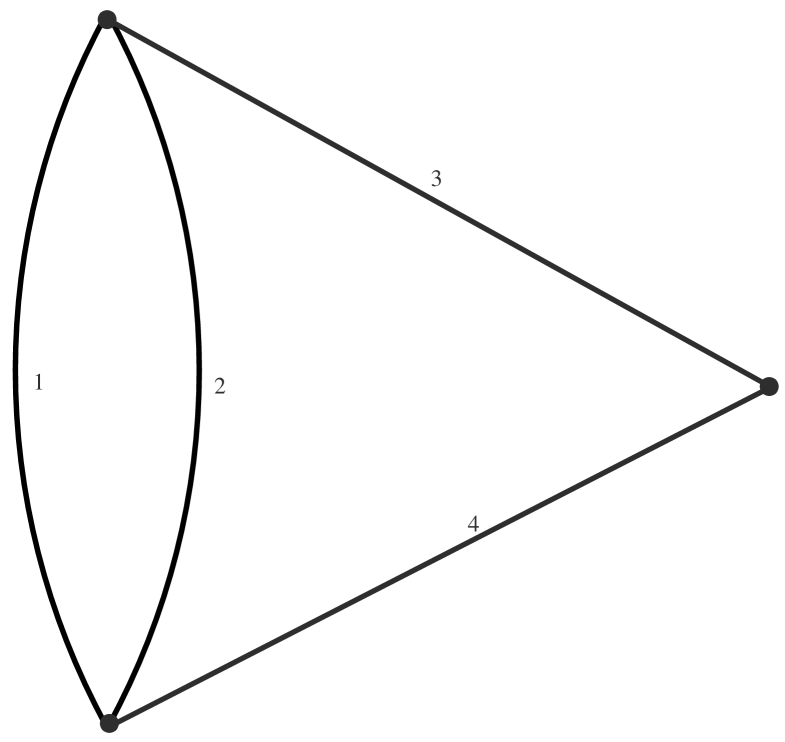
Let be the projective space of lines in which we view as an algebraic variety with homogeneous coordinates . Let be a homogeneous polynomial of some degree , and let be the hypersurface defined by . We assume the coefficients of are all real and . Let be the topological -chain (simplex) in , where refers to homogeneous coordinates. We will also use the notation . Our assumption about coefficients implies
| (1.4) |
where runs through all coordinate coordinate linear spaces contained in (see (see Fig.1)).

The genesis of the renormalization problem in physics is the need to assign values to integrals
| (1.5) |
where is an algebraic -form on with poles along . The problem is an important one for physical applications, and there is an extensive literature (see, for example, [10, 22, 21]) focusing on practical formulae to reinterpret (1.5) in some consistent way as a polynomial in . (Here parametrizes a deformation of the integration chain. As a first approximation, one can think of when has a logarithmic pole at .)
A similar problem arises in pure mathematics in the study of degenerating varieties, e.g. a family of elliptic curves degenerating to a rational curve with a node. In the classical setup, one is given a family , where is a disk with parameter . The map is proper (so the fibres are compact). is assumed to be non-singular, as are the fibres . may be singular, though one commonly invokes resolution of singularities to assume is a normal crossing divisor. Choose a basis for the homology of the fibre in some fixed degree . By standard results in differential topology, the fibre space is locally topologically trivial over , and we may choose the classes to be locally constant. If we fix a smooth fibre , the monodromy transformation is obtained by winding around . An important theorem ([7], III,2) says this transformation is quasi-unipotent, i.e. after possibly introducing a root (which has the effect of replacing by ), is nilpotent. The matrix
| (1.6) |
is thus also nilpotent. This is the mathematical equivalent of locality in physics. It insures that our renormalization of (1.5) will be a polynomial in rather than an infinite series. We take a cohomology class which varies algebraically. For example, in a family of elliptic curves , the holomorphic -form is such a class. Note is single-valued over all of . It is not locally constant. The expression
| (1.7) |
is then single-valued and analytic on . Suppose chosen such that the entries of the column vector in (1.7) grow at worst like powers of as . A standard result in complex analysis then implies that (1.7) is analytic at . We can write this
| (1.8) |
Here the are constants which are periods of a limiting Hodge structure. The exponential on the right expands as a matrix whose entries are polynomials in , and the equivalence relation means that the difference between the two sides is a column vector of (multi-valued) analytic functions vanishing at .
We would like to apply this program to the integral (1.5). Let be the coordinate divisor in . Note that the chain has boundary in , so as a first attempt to interpret (1.5) as a period, we might consider the pairing
| (1.9) |
The form is an algebraic -form and it vanishes on for degree reasons, so it does give a class in the relative cohomology group appearing in (1.9) (see the discussion (9.8)-(9.10)). On the other hand, the chain meets (1.4), so we do not get a class in homology. Instead we consider a family of coordinate divisors with . (For details, see section 6.) For there is a natural chain which is what the physicists would call a cutoff. We have and , so is defined. One knows on abstract grounds that the monodromy of
is quasi-unipotent as above ([7], III,§2). The main mathematical work in this paper will be to compute the monodromy of in the specific case of Feynman amplitudes in physics. More precisely, will be a graph hypersurface associated to a graph (section 5). We will write down chains , one for each flag of core (one particle irreducible in physics) subgraphs , representing linearly independent homology classes in . (The combinatorics here is similar to that found in [1], [18].) We will show the monodromy in our case is given by
| (1.10) |
We will then exhibit a nilpotent matrix such that
| (1.11) |
With this in hand, renormalization is automatic for any physical theory for which and its subgraphs are at worst logarithmically divergent after taking out suitable polynomials in masses and momenta. Namely, such a physical theory gives a differential form as in (1.5) and we may repeat the above argument:
| (1.12) |
is single-valued on the punctured disk. The hypothesis of log divergence at worst for subgraphs of will imply that the integrals will grow at worst like a power of as ,(lemma 9.2). Precisely as in (1.8), one gets the renormalization
| (1.13) |
where denotes a (multi-valued) analytic function vanishing at . The renormalization schemes considered here can be characterized by the condition .
Of course, the requirement that a physical theory have at worst log divergences is a very strong constraint. The difficult computations in section 7 show how general divergences encountered in physics can be reduced to log divergences.
Remarks 1.1.
The renormalization scheme outlined above, and worked out
in detail in the following sections, has a number of properties,
some of which may seem strange to the physicist.
(i) It does not work in renormalization schemes which demand counter-terms which are not defined by subtractions at fixed values of masses and momenta of the theory. So conditions on the regulator for example, as in minimal subtraction where one defines the counterterm by projection onto a pole part, are not considered. In such schemes, and for graphs which are worse than log divergent, a topological procedure of
the sort given here can not work. It is necessary instead to modify
the integrand in a non-canonical way.
(ii) On the other hand, our approach is very canonical. It depends on
the choice of a parameter , as any renormalization scheme
must. Somewhat more subtle is the dependence on the monodromy
associated to the choice of a family
of coordinate divisors deforming the given
. We have taken the most evident such monodromy,
moving all the vertices of the simplex. Note that this choice is stable in the sense that a small deformation leaves the monodromy unchanged.
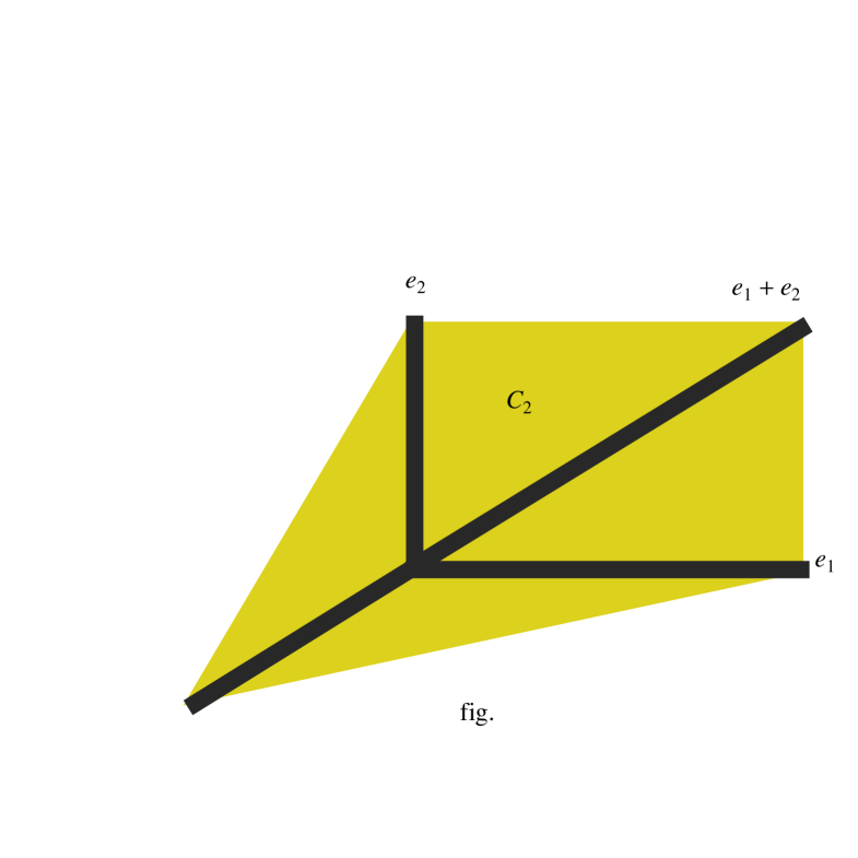
(iii) It would seem that our answer is much more complicated than need
be, because will in general contain far more core subgraphs
than divergent subgraphs. For example, in -theory, the
“dunce’s cap” (see Fig.2)
has only one divergent subgraph, given in
the picture by edges . It has core subgraphs
. From the point of view of renormalization,
this problem disappears. The are tubes, and the
integral is basically a residue
which will vanish unless is a divergent
subgraph. In (1.12), the column vector of integrals will consist
mostly of ’s and the final regularization (1.13) will involve
only divergent subgraphs.
(iv) An important property of the theory is the presence of a limiting mixed Hodge structure. The constants on the right hand
side of (1.8) are periods of a mixed Hodge structure called
the limiting MHS for the degeneration. One may hope that the
tendency for Feynman amplitudes to be multi-zeta numbers [4]
will some day be understood in terms of this Hodge structure. From
the point of view of this paper, the vector space
spanned by and the is invariant under
the monodromy. One may ask whether the image of in the
limiting MHS spans a sub-Hodge structure. If so, we would expect
that this HS would be linked to the multi-zeta numbers. Note that
is highly non-trivial even when has no
subdivergences. This is an essentially new invariant which
comes out of the monodromy. See section (9.2) for a
final discussion of our viewpoint.
(v) There are a number of renormalization
schemes in physics, some of which are not compatible with our
approach. One general test is that our scheme depends only on the
graph polynomials of . For example, suppose where the meet at a single
vertex. Then the renormalization polynomial in our theory
yields for will be the product of the renormalizations
for the .
Most of the mathematical work involved concerns the calculation of monodromy for a particular topological chain. It is perhaps worth taking a minute to discuss a toy model. Suppose one wants to calculate , where . The integral diverges, so instead we consider as a function of for . If we take the path to be a great circle, then as winds around , the path will get tangled in the singularity of at . Assuming we do not understand the singularities of our integral far from , this could be a problem. Instead we chose our path to follow the small circle from to and then the positive real axis from to . The variation of monodromy is the difference in the paths for and . In this case, it is the circle . If we assume something (at worst superficial log divergence for the given graph and all subgraphs in the given physical theory) about the behavior of near the pole at , then the behavior of our integral for is determined by this monodromy, which is a topological invariant. This is quite different from the usual approach in physics involving complicated algebraic manipulations with . A glance at fig.(10) suggests that our toy model is too simple. We have to work with two scales, . This is because in the more complicated situation, we have to deal with cylinders of small radius , but then we have further to slightly deform the boundaries of the cylinder (cf. fig.(12)).
1.4. Leitfaden
Section 2 is devoted to Hopf algebras of graphs and of trees. These have played a central role in the combinatorics of renormalization. In particular, the insight afforded by passing from graphs to trees is important. Since the combinatorics of core subgraphs is even more complicated than that of divergent subgraphs, it seemed worth going carefully through the construction. Section 3 studies the toric variety we obtain from a graph by blowing up certain coordinate linear spaces in the projective space with homogeneous coordinates labeled by the edges of . The orbits of the torus action are related to flags of core subgraphs of the given graph. In section 4, we use the -structure on our toric variety to construct certain topological chains which will be used to explicit the monodromy. Section 5 recalls the basic properties of the graph polynomial and the graph hypersurface . The crucial point is corollary 5.3 which says that the strict transform of on our toric blowup avoids points with coordinates . Any chain we construct which stays close to the locus of such points necessarily is away from and hence also away from the polar locus of our integrand. Section 6 computes the monodromy of our chain. Section 7 considers how to reduce Feynman amplitude calculations as they arise in physics, including masses and momenta as well as divergences which are worse than logarithmic, to the basic situation where limiting methods can apply. In section 8 we calculate the nilpotent matrix which is the log of the monodromy transformation, and in section 9 we prove the main renormalization theorem in the log divergent case, to which we have reduced the theory.
2. Hopf algebras of trees and graphs
2.1. Graphs
In this section we bring together material on graphs and the graph Hopf algebra which will be used in the sequel. We also discuss Hopf algebras related to rooted trees and prove a result (proposition 2.5) relating the Hopf algebra of core graphs to a suitable Hopf algebra of labeled trees. Strictly speaking this is not used in the paper, but it provides the best way we know to understand flags of core subgraphs, and these play a central role in the monodromy computations. Trees labeled by divergent subgraphs have a long history in renormalization theory [12], [13].
A graph is determined by giving a finite set of half-edges, together with two further sets (edges) and (vertices) and surjective maps
| (2.1) |
(Note we do not allow isolated vertices.) In combinatorics, one typically assumes all fibres consist of exactly two half-edges ( an internal edge), while in physics the calculus of path integrals and correlation functions dictates that one admit external edges with . If all internal edges of are shrunk to , the resulting graph (with no internal edges) is called the residue . In certain theories, the vertices are decomposed into different types , and the valence of the vertices in , , is fixed independent of .
We will typically work with labeled graphs which are triples . We refer to as the set of edges.
A graph is a topological space with Betti numbers and . We say is connected if . Sometimes is referred to as the loop number.
A subgraph is determined (for us) by a subset . We write for the quotient graph obtained by contracting all edges of to points. If is not connected, is different from the naive quotient . If , we take to be the empty set. It will be convenient when we discuss Hopf algebras below to have the empty set as a graph.
Also, for a single edge, we have the contraction . In this case we also consider the cut graph obtained by removing and also any remaining isolated vertex.
A graph is said to be core ( in physics terminology) if for any edge we have .
A cycle is a core subgraph such that . If is core, it can be written as a union of cycles (see e.g. the proof of lemma 7.4 in [2]).
2.1.1. Self-energy graphs
Special care has to be taken when the residue of a connected component of some subgraph consists of two half-edges connected to a vertex, . Such graphs are called self-energy graphs in physics. In such a situation, if the internal edges of contract to a point, we are left with two edges in , which are connected at this point . It might happen that the theory provides more than one two-point vertex. In fact, for a massive theory, there are two two-point vertices provided by the theory corresponding to the two monomials in the Lagrangian quadratic in the fields, we call them of mass and kinetic type. represents then a sum over two graphs by summing over the two types of vertices for that point . (see Fig.(3) for an example).

The edges and vertices of various types have weights. We set the weight of an edge to be two, the weight of a vertex with valence greater than two is zero, the weight of a vertex of mass type is zero, the weight of the kinetic type is +2.
Then, the superficial degree of divergence for a connected core graph is
| (2.2) |
where is the set of vertices of kinetic type, and the set of internal edges. , the set of interaction vertices (for which we assume we have only one type) does not show up as they have weight zero, nor does . By we denote the cardinality of these sets.
Note that a graph which has one two-point vertex labeled (of mass type) which appears after contracting a self-energy subgraph has an improved power-counting as its edge number is . If the two-point vertex is labeled by (kinetic type), it has not changed though: , as the weight of the two-point vertex compensates for the weight of the extra propagator. Quite often, in massless theories, one then omits the use of these two-point vertices altogether.
2.2. Hopf algebras of graphs
Let be a class of graphs. We assume and that and implies . We say is closed under extension if given we have
| (2.3) |
Easy examples of such classes of graphs are , and , where is log divergent (in theory) if it is core and if further for every connected component . (Both examples are closed under extension by virtue of the identity .) Examples which arise in physical theories are more subtle. Verification of (2.3) requires an analysis of which graphs can arise from a given Lagrangian. To verify satisfies (2.3) one must consider self-energy graphs and the role of vertices of kinetic type as discussed above.
In particular, in massless theory divergent graphs are closed under extension, and so is the class of graphs for which . Note that this may contain superficially convergent graphs if there are sufficiently many two-point vertices of mass type. It pays to include them in the class of graphs to be considered, which enables one to discuss the effect of mass in the renormalization group flow.
Associated to a class which is closed under extension as above, we define a (commutative, but not cocommutative) Hopf algebra as follows. As a vector space, is freely spanned by isomorphism classes of graphs in . (A number of variants are possible. One may work with oriented graphs, for example. In this case, the theory of graph homology yields a (graded commutative) differential graded Hopf algebra. One may also rigidify by working with disjoint unions of subgraphs of a given labeled graph.) becomes a commutative algebra with and product given by disjoint union. Define a comultiplication :
| (2.4) |
One checks that (2.3) implies that (2.4) is coassociative. Since is graded by loop numbers and each is finite dimensional, the theory of Hopf algebras guarantees the existence of an antipode, so is a Hopf algebra.
If with Hopf algebras ( e.g. take to be core graphs, and divergent core graphs) then the map obtained by sending if is a homomorphism of Hopf algebras. For example, the divergent Hopf algebra carries the information needed for renormalization [13], while the core Hopf algebra determines the monodromy. In terms of groupschemes, one has is a closed subgroupscheme, and renormalization can be viewed as a morphism from the affine line with coordinate to . Already here we use that for divergent graphs with , we can evaluate them as polynomials in masses and external momenta with coefficients determined from log divergent graphs, see below.
Let be core graphs (a similar discussion will be valid for other classes of graphs) and let be vertices. Let where the two graphs are joined by identifying . Then is core (cf. proposition 3.2). Further, core subgraphs all arise as the image of for core. Thus
| (2.5) |
It follows that the vector space spanned by elements as above satisfies . Since is an ideal, we see that is a commutative Hopf algebra. Roughly speaking, is obtained from by identifying one vertex reducible graphs with products of the component pieces.
Generalization to theories with more vertex and edge types are straightforward.

Fig.(4) gives the wheel with three spokes. This graph, which in theory (external edges to be added such that each vertex is four-valent) has a residue for conceptual reasons [2], has a coproduct (we omit edge labels and identify terms which are identical under this omission, which gives the indicated multiplicities)
| (2.6) | |||||
For example, the three possible labelings for the four-edge cycle in the third line are , and . While the graph has a non-trivial coproduct in the core Hopf algebra, it is a primitive element in the renormalization Hopf algebra. It is tempting to hope that the core coproduct relates to the Hodge structure underlying the period which appears in the residue of this graph.
2.3. Rooted tree Hopf algebras [12], [3]
We introduce the Hopf algebra of decorated non-planar rooted trees using non-empty finite sets as decorations (decorations will be sets of edge labels of Feynman graphs below) to label the vertices of the rooted tree Hopf algebra . Products in are disjoint unions of trees (forests). We write the coproduct as
| (2.7) |
Edges are oriented away from the root and a vertex which has no outgoing edge we call a foot. An admissible cut is a subset of edges of a tree such that no path from the root to any vertex of traverses more than one element of that subset. Such a cut separates into at least components. The component containing the root is denoted , and the product of the other components is .
A ladder is a tree without side branching. Decorated ladders generate a sub-Hopf algebra . A general element in is a sum of bamboo forests, that is disjoint unions of ladders. Decorated ladders have an associative shuffle product
| (2.8) |
where denotes the ordered set of decorations for and is the set of all ordered sets obtained by shuffling together and .
Lemma 2.1.
Let be the ideal generated by elements of the form . Then .
Proof.
Write where is the length of and (resp. ) is the bottom (resp. top) subladder of length . Then
| (2.9) | |||
Consider pairs of indices in (2.9) and write . Among the pairs we consider the subset for which the first elements of the ordered set consist of a shuffle of the decorations on the ladders . It is clear that the remaining elements of will then run through shuffles of the decorations of , so
| (2.10) |
∎
Remark 2.2.
Any bamboo forest is equivalent mod to a sum of stalks. Indeed, one has e.g.
| (2.11) |
For any decoration , one has an operator [3]
| (2.12) |
which carries any forest to the tree obtained by connecting a single root vertex with decoration to all the roots of the forest. This operator is a Hochschild 1-cocycle, i.e.
| (2.13) |
Let be the smallest ideal containing the ideal as in lemma 2.1 and stable under all the operators . Generators of as an abelian group are obtained by starting with elements of and successively applying for various and multiplying by elements of . It follows from (2.13) that . Define
| (2.14) |
A flag in a core graph is a chain
| (2.15) |
of core subgraphs. Write for the collection of all maximal flags of . One checks easily that for a maximal flag, . Let us consider an example.
| (2.16) | |||||
| (2.17) | |||||
| (2.18) | |||||
| (2.19) | |||||
| (2.20) | |||||
| (2.21) | |||||
| (2.22) | |||||
| (2.23) | |||||
| (2.24) | |||||
| (2.25) | |||||
| (2.26) | |||||
| (2.27) |
are the twelve flags for the graph given in Fig.(5). We omitted the edge labels in the above flags. Note that only the first two , (2.16,2.17) are relevant for the renormalization Hopf algebra to be introduced below.

To the flag we associate the ladder with vertices decorated by . (More precisely, the foot is decorated by and the root by .). Define
| (2.28) |
Here the set of labels will be the set of subsets of graph labels.
Lemma 2.3.
The map is a homomorphism of Hopf algebras.
Proof.
For a flag let be the bottom vertices with the given labeling, and let be the top vertices with the quotient labeling gotten by contracting the core graph associated to the bottom vertices. For a core subgraph, define . There is a natural identification
| (2.29) |
We have
| (2.30) |
On the other hand
| (2.31) |
The assertion of the lemma is that there is a correspondence
| (2.32) |
This is clear. ∎
In fact, the tree structure associated to a maximal flag of is rather more intricate than just a ladder. Though we do not use this tree structure in the sequel, we present the construction in some detail to help in understanding the difference between the core and renormalization Hopf algebra.
We want to associate a forest to the flag , and we proceed by induction on . We can write in such a way that all the are core and one vertex irreducible, and such that . This decomposition is unique. If it is nontrivial, we define where is the induced flag from on . We now may assume is one vertex irreducible. If the in our flag are all one vertex irreducible, we take to be a ladder as above. Otherwise, let be maximal such that is one vertex reducible. By induction, we have a forest . To define , we glue the foot of the ladder with decorations to all the roots of . (For an example, see figs.(6) and (7).)

Lemma 2.4.
Let where and the are core. Assume . Then, viewing flags as sets of core subgraphs, ordered by inclusion, there is a correspondence between and shuffles of the .
Proof.
One checks easily that the can have no edges in common. Further, there is a correspondence between core subgraphs and collections of core subgraphs . Here, the dictionary is given by and . The assertion of the lemma follows. ∎

As a consequence of lemma 2.4 we may partition the flags associated to a core as follows. Given , Let be maximal in the flag such that is -vertex reducible. The flag induces a flag on , and we know that it is a shuffle of flags on where as in the lemma. We say two flags are equivalent, , if and agree at and above, and if they simply correspond to two different shuffles of the flags . We now have
| (2.33) |
Indeed, is obtained by successive operations applied to the forest . The latter, by remark 2.2, coincides with the righthand side of (2.33). We conclude
Proposition 2.5.
With notation as above, there exist homomorphisms of Hopf algebras
| (2.34) |
Here is the sum over equivalence classes of flags as above. We will barely use in the following, and introduced it for completeness and the benefit of the reader used to it.
2.4. Renormalization Hopf algebras
In a similar manner, one may define homomorphisms
| (2.35) |
for any one of the renormalization Hopf algebras obtained by imposing restrictions on external leg structure. For a graph , let, as before, the residue of , , be the graph with no loops obtained by shrinking all its internal edges to a point. What remains are the external half edges connected to that point (cf. section 2.1). Note that ”doubling” an edge by putting a two-point vertex in it does not change the residue.
In theory for example, graphs have external legs, with . For a renormalizable theory, there is a finite set of external leg structures such that we obtain a renormalization Hopf algebra for that set.
For example, for massive theory, there are three such structures: the four-point vertex, and two two-point vertices, of kinetic type and mass type.
Let us now consider flags associated to core graphs. Such chains correspond to decorated ladders, and the coproduct on the level of such ladders is a sum over all possibilities to cut an edge in such a ladder, splitting the chain
| (2.36) |
So let us call such an admissible cut renormalization-admissible, if all core graphs , obtained by the cut have residues in .
The set of renormalization-admissible cuts is a subset of the admissible cuts of a core graph, and the coproduct respects this. Hence the renormalization Hopf algebra is a quotient Hopf algebra of the core Hopf algebra.
If we enlarge the set to include other local field operators appearing for example in an operator product expansion we get quotient Hopf algebras between the core and the renormalization Hopf algebra.
2.5. External leg structures
External edges are usually labeled by data which characterize the amplitude under consideration. Let be such data. For graphs with a given residue , there is a finite set of possible data . A choice of such data determines a labeling of the corresponding vertex to which a subgraph shrinks. Let be that co-graph with the corresponding vertex labeling.
One gets a Hopf algebra structure on pairs by using the renormalization coproduct by setting . We regard the decomposition into external leg structures as a partition of unity and write
| (2.37) |
In our applications we only need this for (sub)graphs with , and the use of these notions will become clear in the applications below.
3. Combinatorics of blow-ups
We consider with fixed homogeneous coordinates . Suppose given a subset . Assume and that has the property that whenever with , then . For we write for the coordinate linear space defined by . Write . We see that
| (3.1) |
We can stratify the set taking to be the set of all minimal elements (under inclusion) of . More generally, will be the set of minimal elements in .
Proposition 3.1.
(i) Elements in are all disjoint, so
we may define to be the variety defined by blowing up
elements in on . We do not need to specify an order
in which to
perform the blowups.
(ii) More generally, the strict transforms of elements in to
the space obtained by successively blowing the strict
transform of are disjoint, so we may
inductively define to be the successive blowup of the
.
(iii) Let correspond to the blowup of . ( is the unique exceptional divisor with image in .)Then if and
only if after possibly reordering, we have inclusions
.
(iv) The total exceptional divisor is a normal
crossings divisor.
(v) Let be a coordinate linear space. Assume for any . Then satisfies (3.1). The strict transform of in
is obtained by blowing up elements of on as in (i) and (ii)
above.
Proof.
If and , then for some . This means that when we get to the -th step, has already been blown up, so the strict transforms of the are disjoint, proving (ii). For , follows from the above argument. Conversely, if we have strict inclusions among the , we may write (abusively) for the projective space with homogeneous coordinates the homogeneous coordinates on vanishing on . The exceptional divisor on the blowup of is identified with . A straightforward calculation identifies nonempty open sets (open toric orbits in the sense to be discussed below) in and
| (3.2) |
The remaining parts of the proposition follow from the algorithm in [8]. ∎
For us, sets as above will arise in the context of graphs. Recall in 2.1 we defined the notion of core graph.
Proposition 3.2.
Let be a graph, and let be core subgraphs. Then the union is a core subgraph.
Proof.
Removing an edge increases the Euler-Poincaré characteristic by . If doesn’t drop, then either increases (the graph disconnects when is removed) or has a unary vertex so removing drops the number of vertices. Suppose is an edge of (assumed core). Then cannot have a unary vertex. If, on the other hand, removing disconnects , then since the are core what must happen is that each has precisely one vertex of . But this would imply that is not core, a contradiction. ∎
To a graph we may associate the projective space with homogeneous coordinates labeled by the edges of . Let be a core graph. A coordinate linear space is a non-empty linear space defined by some subset of the homogeneous coordinate functions, . Define to be the set of coordinate linear spaces in such that the corresponding set of edges is the edge set of a core subgraph . It follows from proposition 3.2 that satisfies condition (3.1), so the iterated blowup
| (3.3) |
as in proposition 3.1 is defined. Define
| (3.4) |
Lemma 3.3.
Suppose with coordinates . Let be defined by . Let be the blowup of . Then the exceptional divisor is identified with . Further induce coordinates on the vertical fibres and give homogeneous coordinates on .
Proof.
This is standard. One way to see it is to use the map . (Here, and in the sequel, denotes a point in homogeneous coordinates.) This extends to a map on :
| (3.5) |
The resulting map . ∎
It will be helpful to better understand the geometry of . Let be the standard one dimensional algebraic torus. Define where the quotient is taken with respect to the diagonal embedding. For all practical purposes, it suffices to consider complex points
| (3.6) |
A toric variety is an equivariant (partial) compactification of . In other words, is an open set, and we have an extension of the natural group map
| (3.7) |
For example, is a toric variety for a torus . Canonically, we may write More important for us:
Proposition 3.4.
(i) is a toric variety for
.
(ii) The orbits of on are in correspondence with
pairs . Here is a (possibly empty) subforest
(subgraph with
) and the are core subgraphs of . We
require that the image of in
be a subforest for each .
(cf. (3.2)). The orbit associated to such a pair is
canonically identified with the open orbit in the toric variety
.
Proof.
A general reference for toric varieties is [9]. The fact (i) that is a toric variety follows inductively from the fact that the blowup of an invariant ideal in a toric variety is toric. Indeed, the torus acts on and hence on the blowup .
We recall some toric constructions. Let , and let . We have canonically where is the group ring of the lattice . A fan (op. cit., 1.4, p. 20) is a finite set of convex cones in satisfying certain simple axioms. To a cone one associates the dual cone (op. cit. p. 4)
| (3.8) |
(resp. the semigroup ). The toric variety associated to the fan is then a union of the affine sets . For example, our has rank . There are evident elements determined by the edges of . Let be the cone spanned by all edges except . The spanning edges for form a basis for which implies that . Since all the coordinate rings lie in (i.e. ), one is able to glue together the . The resulting toric variety associated to the fan is canonically identified with .
Remark 3.5.
Our toric varieties will all be smooth (closures of orbits in smooth toric varieties are smooth), which is equivalent ([9], §2) to the condition that cones in the fan are all generated by subsets of bases for the lattice . Faces of these cones are in correspondence with subsets of the generating set.
In general, the orbits of the torus action are in correspondence with the cones in the fan (op. cit. 3.1, p.51). The subgroup of generated by corresponds to the subgroup of which acts trivially on the orbit. For example, in the case of projective space , there are cones of dimension corresponding to the fixed points . For any , the cone spanned by the edges of corresponds to the orbit . Let be a coordinate linear space in associated to a subgraph . It follows from lemma 3.3 that the exceptional divisor in the blowup of can be identified with
| (3.9) |
Let , and write . The subgroup determines a -parameter subgroup . It follows from (3.9) that acts trivially on . One has for all , where is the cone generated by the edges of . For all we define a subcone to be spanned by together with all edges of except . The fan for is then
| (3.10) |
Note that is not a cone in the fan for . More generally, let be the fan for . Certainly, will contain as cones the half-lines for all core subgraphs as well as the . but we must make precise which subsets of this set of half-lines span higher dimensional cones in . By general theory, the cones correspond to the nonempty orbits. In other words,
| (3.11) |
span a cone in if and only if the intersection
| (3.12) |
where is the exceptional divisor corresponding to and is the strict transform of the coordinate divisor in . To understand (3.12), consider the simple case . We have a core subgraph , and an edge of . We know by lemma 3.3 that . If is an edge of , then . Otherwise
One (degenerate) possibility is that is an edge of which forms a loop (tadpole). In this case, is itself a core subgraph of , and the divisor should be treated as one of the exceptional divisors . Thus, we omit this possibility. Another possibility is that , but that the image of in forms a loop. In this case, is a core subgraph, so the linear space gets blown up in the process of constructing . But blowing separates and , so the intersection of the strict transforms of and in is empty. The general argument to show that (3.12) is empty if and only if the conditions of (ii) in the proposition are fulfilled is similar and is left for the reader. Note that the case where there are no divisors follows from proposition 3.1(iii). ∎
We are particularly interested in orbits corresponding to filtrations by core subgraphs . Let be the closure of this orbit. We want to exhibit a toric neighborhood of which retracts onto as a vector bundle of rank . As in the proof of proposition 3.4 we have . The cone spanned by the lies in the fan . For cones we write if is a subcone of . By the general theory, this will happen if and only if is a subcone which appears on the boundary of . The orbit corresponding to will then appear in the closure of the orbit for .
Proposition 3.6.
With notation as above, Let be the subset of cones such that we have for some . Write for the open toric subvariety corresponding to the subfan . We have . Further there is a retraction realizing as a rank vector bundle over which is equivariant for the action of the torus .
Proof.
One has the following functoriality for toric varieties [9], §1.4. Suppose is a homomorphism of lattices (finitely generated free abelian groups). Let be fans in . Suppose for each cone there exists a cone such that . Then there is an induced map on toric varieties . Let as above, and . One has the evident surjection . We take as fan . The closure of the orbit corresponds to the fan in given by the images of all cones (op. cit. §3.1). Such a is generated by , and there are no linear relations among these elements (remark 3.5). A subcone is generated by a subset . The image is simply the cone in generated by the images of the ’s. If we have another cone in with the same image in , it will have generators say together with some of the ’s. Reordering the ’s, we find that there are relations
| (3.13) |
with . It follows that the cones in spanned by and meet in a subset strictly larger that the cone spanned by the . By the fan axioms, the intersection of two cones in a fan is a common face of both, so these two cones coincide, which implies . In particular, for each cone in , there is a unique minimal cone in lying over it. This is the hypothesis for [19], p. 58, proposition 1.33. One concludes that the map induced by the map is an equivariant fibration, with fibre the toric bundle associated to the fan generated by the . This toric variety is just affine -space, so we get an equivariant -fibration over . Any such fibration is necessarily a vector bundle with structure group . Indeed, this amounts to saying that any automorphism of the polynomial ring which intertwines the diagonal action of is necessarily of the form with . ∎
Remark 3.7.
We will need to understand how these constructions are compatible. Let be a closed orbit corresponding to a cone as above, and let be a smaller closed orbit corresponding to a larger cone . (The correspondence between cones and orbits is inclusion-reversing.) As above we have a toric variety and a retraction . The fan for is given by the set of cones in such that
| (3.14) |
It follows that , so is an open subvariety. Let be the image of the composition . Then is the open toric subvariety of corresponding as above to the closed orbit , and we have a retraction . One gets commutative diagrams
| (3.15) |
and
| (3.16) |
Remark 3.8.
Using the toric structure, one can realize these vector bundles as direct sums of line bundles corresponding to characters of the tori acting on the fibres.The inclusion on the top line of (3.16) corresponds to characters which act trivially on all of .
Remark 3.9.
(compare proposition 3.4). Given a flag of core subgraphs
| (3.17) |
let be defined by the edge variables for edges in , so we have . For a coordinate linear space, let be the subtorus where none of the coordinates vanish. Then the orbit associated to (3.17) is
| (3.18) |
(Here the notation is as in (3.2).)
4. Topological Chains on Toric Varieties
One can define the notion of non-negative real points and positive real points . For a torus for some we take
A toric variety can be stratified as a disjoint union of tori . Define
| (4.1) | |||
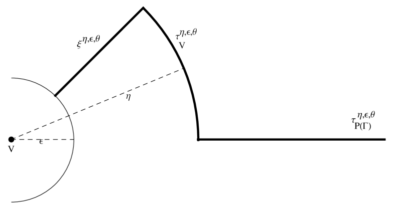
where is the open orbit. Let be the closure of the orbit associated to a flag (3.17), and let be the subtorus acting trivially on . Let be the vector bundle as in proposition 3.6. We write as a direct sum of line bundles, where each is equivariant for . Let be the maximal compact subgroup. Note that one has a canonical identification associated to the -parameter subgroups of generated by . In particular, the identification is canonical as well. For all closed orbits we may fix metrics on the which are compatible under inclusions (3.16) and are (necessarily) invariant under the action of . We fix also a constant . We can then define to be the product of the circle bundles of radius embedded in the . becomes a principal bundle over with structure group . Note that contains a unique point in every fibre of over a point of . Let be another constant. We need to define a chain . We consider closures of codimension orbits in . For each such we have an open and a retraction which is a line bundle with a metric. The fibres of have a canonical coordinate . If corresponds to an intersection of with another exceptional divisor , then we remove from each fibre of over the locus where . If, on the other hand corresponds to an intersection of V with one of the (i.e. with a strict transform of one of the coordinate divisors), then we remove the locus . Repeating this process for each (i.e. for each irreducible toric divisor in ), we obtain a compact which stays away from the boundary components. (Here ”boundary components” are exceptional divisors together with strict transforms of coordinate divisors.)
Example 4.1.
Consider the case . Let , and let
be the original integration chain. We have defined by excising away points within a distance of from an or from the strict transform of a coordinate divisor . (cf. fig.(8)). It is a manifold with corners.
Define to be the inverse image of in . The fibres of over are products with a canonical origin at the point where this fibre meets . For an angle , we can thus define to be swept out by the origin in each fibre under the action of . The chains have -dimension which is equal to the complex dimension of and .
Example 4.2.
Here is an example which is too simple to correspond to any graph, but is sufficient to clarify the toric picture. Take
| (4.2) |
in with coordinates . Take to be the blowup of . Let be the exceptional divisor, and let be the strict transform of . Note that is already a divisor so it is not necessary to blow up again. Take . The fan for is fig.(9).
The cone , so the fan is the subset of cones lying in the first quadrant. The toric variety is with blown up. It projects down onto as a line bundle. is then a circle bundle over . has two suborbits and , where is the strict transform of the divisor in . We may interpret as a coordinate on , so and . We have and . The real chain , and is the -bundle of radius over . On the other hand, corresponds to the cone labeled in fig.(9), and the fan is just itself. The toric variety is a rank vector bundle over the point . We have . In this case is simply the point , and . In local coordinates around given by eigenfunctions for the torus action we have
| (4.3) | |||
We want now to establish a basic formula for the boundary of the chains . Here runs through the closures of orbits in associated to flags of core subgraphs (3.17). We include the big orbit . We write . We may express the boundary chains locally (in fact Zariski-locally) in coordinates which are eigenfunctions for the torus action. It is clear (cf. (4.3)) that boundary terms are obtained by setting a suitable one of these coordinates to be constant: either or or . (The presence of in the first line of (4.3) simply means that the appropriate coordinate near that point is .)
Proposition 4.3.
For a suitable orientation, the boundary
| (4.4) |
will contain no chains with one coordinate constant .
Proof.
(Cf. fig.(10) ). For a given boundary term, we can choose local eigenfunction coordinates such that be boundary term is given by . We take the chains to be oriented in some consistant way by this ordering of coordinates. (Note that these coordinates are defined on a Zariski open set. The obstruction to choosing consistent orientations for various open sets is a class in the first Zariski cohomology of with constant -coefficients. Since this cohomology group vanishes, we can choose such consistent orientations.) If contains a term with , there are two possibilities. Either is a real coordinate on or it is a circular coordinate. If is a real coordinate, then the fact that appears in the boundary means that locally defines a codimension orbit closure . In , will appear as a circular coordinate. Since , the same chain will appear in and in and will cancel in (4.4). If, on the other hand, is a circular coordinate, then for suitable ordering of coordinates, the chain will be an -bundle over a chain contained in the locus where certain coordinates . But then (4.4) will contain another chain which is an -bundle over , and the boundary components involving will occur with opposite signs and will cancel. ∎
The boundary chain (4.4) is an -chain involving two scales . We want to construct an -chain which amounts to a scaling . To do this, we construct a vector field on . Let be the exceptional divisor. will be outside a neighborhood of . Locally, at a point on which is close to divisors we have coordinates which are eigenfunctions for the torus action such that locally . Locally we will take to be radial and inward-pointing in each . We glue these local ’s using a partition of unity. ”Flowing” the -chain (4.4) along this vector field yields an -chain . If this is done with care, we can arrange
| (4.5) |
Here means that the two sides differ by a chain lying in an -neighborhood of the strict transform of the coordinate divisor in . Another important property of the chain is
Lemma 4.4.
.
Proof.
The point is that except for the case , and is independent of . (See fig.(10)).
∎
Define the chain . We have
| (4.6) |
Note that , i.e. all chains involving at least one circular variable die at . We define the variation,
| (4.7) |
It is a sum of “-tubes” over all .
5. The Graph Hypersurface
Associated to a graph with edges, one has the graph polynomial
| (5.1) |
where runs through spanning trees of . This polynomial has degree . For more detail, see [2] and the references cited there. Let be the graph hypersurface in . For , let be defined by . Let be the subgraph with edges in . Note the dictionary is inclusion reversing.
Lemma 5.1.
(i) if and only
if .
(ii) If , there exists a unique such that and such that
moreover is a core graph.
(iii) We have in (ii) that where runs through all
minimal subsets of such that .
(iv) , where is a coordinate linear space not
contained in .
Proof.
These assertions are straightforward from the results in [2], section 3. Note that (iv) justifies our strategy of only blowing up core subgraphs. ∎
We have seen (remark 3.4) that our blowup is stratified as a union of tori indexed by pairs
| (5.2) |
where is a suitable subforest and the are core.
Proposition 5.2.
(i) As in proposition 3.4, the torus corresponding to (5.2) is
| (5.3) |
Here , where .
(ii) The strict transform of in meets the
stratum (5.3) in a union of pullbacks
| (5.4) |
Here the are the projections to the various subtori in (5.3), and denotes the restriction of the corresponding graph hypersurface to the open torus in the projective space.
Proof.
Let be a subgraph and let . Assume , so . Let be the blowup of . Let be the exceptional divisor, and let be the strict transform of . The basic geometric result (op. cit. prop. 3.5) is that and
| (5.5) |
The assertions of the proposition follow by an induction argument. ∎
Corollary 5.3.
The strict transform of in does not meet the non-negative points (4.1).
Proof.
Remark 5.4.
The Feynman amplitude is obtained by calculating an integral over with an integrand which has a pole along . Again using that is a sum of monomials with non-negative coefficients, one sees from lemma 5.1 that
| (5.6) |
where with a core subgraph. The iterated blowup is exactly what is necessary to separate the non-negative real points from the strict transform of .
Remark 5.5.
The points where have some remarkable properties. It is shown in [20] that for any angular sector with angle , at any complex projective point such that the and all the lie in .
6. Monodromy
Let be the -th coordinate vector. Define
Fix a positive constant and choose with and . We assume the are algebraically generic. Write . Define (cf. fig.(11))
| (6.1) |

We write and for the images of these chains in . Of course, as above, and we know that . Here is as in (3.4).
Lemma 6.1.
Let be a neighborhood of in and let be a neighborhood of . Then there exists such that implies that for all , we have and .
Proof.
We have . By compacity, for . Again by compacity, if we shrink we will have . ∎
Remark 6.2.
Write for the projective span of the points
and let . Thus, and we may consider the monodromy for . More precisely, renormalization in physics involves an integral over the chain . The integrand has poles along . Since , the integral is possibly divergent. On the other hand, by corollary 5.3, the chain does not meet and so represents a singular homology class
| (6.2) |
(Since all , it follows that , and points in have all coordinates .) We consider the topological pairs as a family over the circle and we continuously deform our chain to a family of chains on with boundary on . (We will not be able to take because this chain can meet .) The monodromy map is an automorphism of (6.2) obtained by winding around the circle: . We will calculate and see that it determines in a natural way the renormalization expansion we want.
Recall we have , and , where is the strict transform of and is the exceptional divisor. (The are closures of orbits associated to core subgraphs of .) We may transfer our monodromy problem to . is in general position with respect to the blowups, so we obtain a family of divisors on . Since , we have an isomorphism of topological pairs
| (6.3) |
In section 4 we have defined chains on . These chains sit on (or, in the case of , within) various -bundles over where the have radius with respect to a chosen metric. From corollary 5.3 it follows that for , none of these chains meets . By construction, these chains do not meet , so they may be identified with chains on . We claim that a small modification of the chains will represent the monodromy chains . The monodromy chains should have boundary on . On the other hand, the chains were cut off so they had boundaries on tubes a distance from the toric divisors given by the strict transforms of the (see fig.(12)).

We must “massage” these brutal cutoffs to get them into . Our chains sit on tubes or products of tubes or products of tubes of radius which we can think of as lying on . Since , when we deform the homotopy type of the circles, or product of circles where these divisors intersect the tubes doesn’t change. This may seem strange because while is in general position with respect to , but the intersections with a hollow tubular neighborhood of are canonically homotopic. Indeed, we may take to correspond to a point in a small contractible disk in the moduli space for coordinate simplices around the point corresponding to . The canonical path up to homotopy between the two points in moduli will induce the desired homotopy on the intersections. (See fig.(13). The two sets of four dots on the circles are canonically homotopic.).

In more detail, by corollary 5.3, the chains are bounded away from by a bound which is independent of as . Outside of some tubular neighborhood of we may find a space disjoint from such that contains open neighborhoods of both and and such that we have deformation retractions and . Shrinking , we may assume our -cutoffs lie in . We may then use the deformation retract to extend the chain slightly to a chain which bounds on . It remains to consider the chains . Recall these were obtained by flowing the chain inward toward the exceptional divisor , so (cf. fig.(10)). We are in a small neighborhood of hence by corollary 5.3 we are away from . The point to be checked is that the term is very close to so by the same deformation retraction argument as above we can extend the chain to bound on . The subtlety is that we are -close to as well, so we need the distance from to be . Recall (6.1) we have the vertices . The coordinate divisor is determined by these projective points. The projective point does not change if we scale the coordinates by , so the image in of the affine simplex below, parametrized by , will have boundary in :
| (6.4) |
Consider for example where is the orbit closure corresponding to the blowup of . Take in (6.4) so terms in may be neglected for . Take where is chosen so that (say) . As a consequence, . The corresponding projective point can then be written
| (6.5) |
The boundary is given by setting one or more of the . Points in can be approximated by points (6.5) which then deform into . To see this, note that since is a codimension orbit closure, there will locally be one coordinate on near which takes the constant value on (cf. fig.(10)). On the other hand, (6.5) is in homogeneous coordinates on . To transform to near a general point of , one fixes and looks at ratios
| (6.6) |
for . Clearly, at the boundary we will get coordinates which are close to , and one coordinate (corresponding to the local defining equation for ) of the form . The remaining coordinates on are ratios of the . Since , these ratios are again close to . The calculation for orbit closures of codimension in is similar and is left for the reader. We have proven
Proposition 6.3.
With notation as above, the monodromy of the chain is represented by the chains given by modifying the chains to have boundary in . In particular, the monodromy is given by
| (6.7) |
where is the chain defined in section 4 with boundary extended to as above.
It will be convenient to simplify the notation and write
| (6.8) |
7. Parametric representations
In this section we list well-known representations of the Feynman rules and then prepare for a subsequent analysis of short-distance singularities in terms of mixed Hodge structures.
7.1. Kirchhoff–Symanzik polynomials
Let
| (7.1) | |||||
| (7.2) |
be the two homogenous Kirchhoff–Symanzik polynomials [10, 22]. Here, is a spanning tree of the 1PI graph and are disjoint trees which together cover all vertices of . Also, is the sum of all external momenta attached to vertices covered by . Note that can be written as
| (7.3) |
Here, are external momenta attached to and to , and are rational functions of the edge variables only, and the sum is over independent such kinematical invariants where momentum conservation has been taken into account. We extend the definition to the empty graph by , .
Let denote the degree of a polynomial with regard to variables of the graph .
Lemma 7.1.
i) .
ii)
| (7.4) |
with for all core graphs and subgraphs .
iii)
| (7.5) |
with for all core graphs and subgraphs .
Proof: i) by definition, ii) has been proved in [2], iii) follows similarly by noting that the two-trees of are obtained from the spanning trees of by removing an edge. If that edge belongs to , we get . If it belongs to , we get a monomial
with .
Note that it might happen that , if the external momenta flows through subgraphs only. In such a case
(which can lead to infrared divergences) one easily shows .
7.2. Feynman rules
¿From these polynomials one constructs the Feynman rules of a given theory. For example we have in theory for a vertex graph , ,
| (7.6) |
We will write to abbreviate the affine chain of integration.
The integral is over the -dimensional hypercube of positive real coordinates in with a small strip of width removed at each axis. We regard the integrand
| (7.7) |
as a function of the set of internal masses , the set of external momenta (which can be considered as labels on external half-edges) and the set of graph coordinates , and takes values in . We often omit the dependence and abbreviate for all these external parameters of the integrand: . The renormalization schemes we consider are determined by the condition that the Green function shall vanish at a particular renormalization point , so that renormalization becomes an iterated sequence of subtractions
| (7.8) |
We let be the superficial degree of divergence of a graph given as (see also Eq.(2.2) for a refined version)
| (7.9) |
where is the rank of the first Betti homology, the dimension of spacetime which we keep as an integer, the weights of the propagator for edge as prescribed by free field theory and the weight of the vertex as prescribed by the interaction Lagrangian. Note that we can set the width to zero, if the integrand is evaluated on a graph which has no divergent subgraphs.
Throughout, we assume that all all masses and external momenta are in general position so that there are no zeroes in the -polynomial off the origin for positive values of the variables. In particular, we assume that the point is chosen appropriately away from all mass-shell and kinematical singularities. We remind the reader of the notation (section (2.5)) where stores all the necessary detail on how to evaluate the graph .
A special role is played by the evaluations . They set all internal masses and momenta to zero. Note that this leads immediately to infrared divergences: the Feynman integrands are missing the exponential in the numerator, which provides a regulator at large values of the variables, and hence an infrared regulator. The ultraviolet singularities at small values of the variables are taken into account by the renormalization procedure itself, and hence by our limiting mixed Hodge structure. We will eliminate the case below using that evaluates to zero if there is no dependence on masses or external momenta.
7.3. General remarks on renormalization and QFT
We now consider the renormalization Hopf algebra of 1PI Feynman graphs in section (2.4). We use the notation
| (7.10) |
for its coproduct. Also, . Projection into the augmentation ideal on the rhs is written as
| (7.11) |
so that for example the antipode is
| (7.12) |
Furthermore, we introduce a forest notation for the antipode:
| (7.13) |
where the sum is over all forests [for] and the product is over all subgraphs which make up the forest. Here, a forest [for] is a possibly empty collection of proper superficially divergent 1PI subgraphs of which are mutually disjoint or nested. We call a forest [for] maximal if is a primitive element of the Hopf algebra. As edge sets
| (7.14) |
This is in one-to-one correspondence with the representation of the antipode as a sum over all cuts on rooted trees as detailed in section (2.3) above. The integer is the number of edges removed in this representation.
Let us first assume that the graph and all its core subgraphs have a non-positive superficial degree of divergence, so they are convergent or provide log-pole: for all elements in (the complement of) the forests.
As the integrand depends on only through the argument of the exponential, we redefine the second Kirchhoff–Symanzik polynomial as follows:
| (7.15) |
Then, the unrenormalized integrand is
| (7.16) |
With this notation, the renormalized integrand is (in all sums and products over here and in the following, runs from to )
where is the integrand for the counterterm, and , the integrand in the first line, delivers upon integrating Bogoliubov’s operation. Note that this formula (7.3) is just the evaluation
| (7.18) |
which guarantees that the corresponding Feynman integral exists in the limit [13],[15].
This Feynman integral is obtained by integrating from to each edge variable. For the renormalized Feynman integral we can take the limit , while for the -operation
| (7.19) |
and the counterterm
| (7.20) |
the lower boundary remains as a dimension-full parameter in the integral. Note that the result (7.3) above can also be written in the form, typical for renormalization schemes which subtract by constraints on physical parameters:
| (7.21) |
and as
| (7.22) |
using the notation (7.11,7.10). Similarly, for Feynman integrals,
| (7.23) |
When it comes to actually calculating the integral (7.6) (or, in its renormalized form (7.3)), something rather remarkable happens. By lemma 7.1(i), the term in the exponential in these integrals is homogeneous of degree in the edge variables . The assumption means is homogeneous of degree . Making the change of variable , we find
| (7.24) |
Note that is naturally a meromorphic form on the projective space with homogeneous coordinates the . Writing , we see that the renormalized integral can be rewritten up to a term which is as a sum of terms of the form
| (7.25) |
where
| (7.26) |
is the exponential integral. (Here are defined by taking the locus .) As long as , we may allow for fixed . The Euler constant and terms cancel. When the dust settles, we are left with the projective representation for the renormalized Feynman integral
| (7.27) |
Note that the use of is justified as long as the integrand has all subdivergences subtracted, so is in the form, so that lower boundaries in the variables can be set to zero indeed.
By (7.21), this can be equivalently written as
| (7.28) |
in any renormalization scheme which is described by kinematical subtractions .
Remark 7.2.
It will be our goal to replace the affine by the projective in the above. The presence of lower boundaries, which can not be ignored as the integrand has divergent subgraphs, allows this only upon introducing suitable chains as discussed in previous sections.
Next, we relax the case of log-divergence.
7.4. Reduction of graphs with
We start with an example. To keep things simple but not too simple, we consider the one-loop self-energy graph in theory, a scalar field theory with a cubic interaction in six dimensions of space-time. We have
| (7.29) |
We will renormalize by suitable subtractions at chosen values of masses and momenta in the -polynomial. We hence (with subdivergences taken care of by suitable bar-operations in the general case) replace by , as this leaves invariant.
Then the above can be written, with this subtraction, and by the familiar change of variables , and by one partial integration in ,
| (7.30) | |||||
where we expanded the boundary term up to terms constant in , which gave the term in the second line. We discarded already the pure pole term from .
Note that graphs with have . They hence depend on a single kinematical invariant say, , for which we write .
The result in (7.30) leads us to define two top-degree forms. (Here and we still write for the Kirchhoff–Symanzik polynomials regarded as dependent on either or variables below).
| (7.31) |
and
| (7.32) |
so that
There are corresponding affine integrands
| (7.34) | |||||
| (7.35) |
The graph is renormalized by a choice of a renormalization condition for the coefficient of (wave function renormalization), and by the choice of a condition for the mass renormalization. is often still used to denote the pair of those.
| (7.36) |
The mass counterterm is then
| (7.37) |
and the wave-function renormalization is
| (7.38) |
Note the term 1 in the brackets does not involve exponentials.
The corresponding renormalized contribution is
| (7.39) |
The transition from the unrenormalized contribution to the renormalized one is particularly simple upon defining Feynman rules in accordance with external leg structures:
| (7.40) | |||||
| (7.41) |
so that renormalization proceeds as before on log-divergent integrands.
This example extends straightforwardly to the case of having divergent subgraphs. Let us return to theory and define for a core graph with , (so that it is a self-energy graph and hence has only two external legs, and thus a single kinematical invariant ), and graph-polynomials , , the forms
| (7.43) |
| (7.44) |
The corresponding complete affine integrands are immediate replacing by variables, and multiplying by exponentials , with for counterterms.
One finds by a straightforward computation
| (7.45) | |||||
| (7.46) |
and
| (7.47) | |||||
| (7.48) |
We set
| (7.49) |
in the external leg structure notation of section (2.5). We can combine the results for graphs for all degrees of divergence by defining for a log divergent graph with the results above. And that’s that. Well, we have to hasten and say a word about the Feynman rules when the subgraphs have , and hence also about in that case.
We use, with the projection into the augmentation ideal, the notation
| (7.50) |
Let us consider the quotient Hopf algebra given by quadratically divergent graphs: . We write
| (7.51) |
We add , so
| (7.52) | |||||
| (7.53) |
Here the sum is over all terms of the coproduct with the terms being present whenever is quadratically divergent.
Evaluating the terms by decomposes the bar-operation on the level of integrands as follows.
| (7.54) |
where appears because a subtraction of a term, from a quadratically divergent term, precisely delivers those counterterms by our previous analysis. Note that they contain terms which do not have an exponential, as in the example (7.38,7.37). Often, as a two-point vertex of mass type improves the powercounting of the co-graph, we might keep self-energy subgraphs massless, in which case only terms involving contribute.
We are left to decompose the terms denoted . We find by direct computation
| (7.56) | |||||
The terms denoted gives us the final integrand with a corresponding form . if there are no subgraphs with . Note that has the full as an argument in the common exponential,
| (7.57) |
which defines . The rational coefficient has log-poles only for all subgraphs including the ones with .
The terms is considered in variables. We can integrate as before. As the rational part of the integrand factorizes in and variables, we similarly decompose the former into , , variables. We note only appears in the log (after the integration) as a coefficient of , using Lemma (7.1). Partial integration in eliminates the log and delivers a top-degree form for the integration. These terms precisely compensate against the constant terms mentioned above, as , using that .
We hence summarize
Theorem 7.3.
| (7.58) |
It is understood that each counterterm is computed with a subtraction as befits its argument , and forms are chosen in accordance with the previous derivations. Here, is constructed to have log-poles only. As a projective integral this reads
| (7.59) | |||||
Remark 7.4.
Similar formulas can be obtained for the bar-operations and counterterms, with the same rational functions in the integrands, and exponentials , with or as needed.
Remark 7.5.
We have worked with choices of renormalizations for mass and wave functions, . One can actually also define , and for example set masses to zero in all exponentials (), that’s essentially the Weinberg scheme if one then subtracts at .
Remark 7.6.
This all is nicely reflected in properties of analytic regulators. For example in dimensional regularization the identity , , leads to immediately, where now indicates unrenormalized Feynman rules using that regulator.
Remark 7.7.
We are working so far with constant lower boundaries. The chains introduced in previous sections have moving lower boundaries which respect the hierarchy in each flag. We will study that difference in section (9.1).
7.5. Specifics of the MOM-scheme
We define the MOM-scheme by setting all masses to zero in radiative corrections and keeping a single kinematical invariant in the -polynomial, ,
| (7.60) |
Such a situation arises if we set masses to zero (possibly after factorization of a polynomial part from the amplitude as in the Weinberg scheme), and for vertices if we consider the case of zero momentum transfers, or evaluate at a symmetric point , where denotes the external half-edges of . If we want to emphasize the dependence we write . Trivially, . In the MOM-scheme, subtractions are done at , which defines for all graphs. Counter-terms in the MOM-scheme become very simple when expressed in parametric integrals thanks to the homogeneity of the -polynomial. Note that we hence have as we have set all masses to zero.
In a MOM-scheme, renormalized diagrams are polynomials in :
Theorem 7.8.
For all ,
| (7.61) |
Here, .
Proof: Consider a sequence .
This is in one-to-one correspondence with some decorated rooted tree appearing in (2.35). Choose one edge in each decoration and de-homogenize with respect to that edge. We get a sequence of lower boundaries .
Use the affine representation and integrate to obtain the result.
7.5.1. MOM scheme results from residues
In such a scheme, it is particularly useful to take a derivative with respect to . We consider
| (7.62) |
where we evaluate at after taking the derivative. This number, which for a primitive element of the renormalization Hopf algebra is the residue of that graph in the sense of [2], is our main concern for a general graph. It will be obtained in the limit of the limiting mixed Hodge structure we construct.
Remark 7.9.
It is not that this limit would not exist for general schemes. But the limit would be a complicated function of ratios of masses and kinematical invariants, which has a constant term given by the number and beyond that a dependence on these ratios which demands a much finer Hodge theoretic study than we can offer here.
But first we need to remind ourselves how coefficients of higher powers of logarithms of complicated graphs related to coefficients of lower powers of sub- and co-graphs thanks to the renormalization group.
7.5.2. The counterterm
For , we simply use the renormalization group or the scattering type formula. In particular, we have
| (7.63) |
Note that this determines counter-terms by iteration: for a -loop graph, knowledge of all the lower order counterterms suffices to determine all contributions to the -loop counterterm but the lowest order coefficient of . But then, that coefficient is given by the formula
| (7.64) |
which itself only involves counter-terms of less than loops, by the structure of the bar operation.
7.5.3. from co-graphs
We can now summarize the consequences of the renormalization group and our projective representations for parametric representations of Feynman integrals. The interesting question is about the logs which we had in numerators. Thm.(7.3) becomes
Theorem 7.10.
| (7.65) |
This limit is
| (7.66) | |||||
The derivative with respect to can be taken inside the integral in (7.65) if and only if all edges carrying external momentum are in the complement of all edges belonging to divergent subgraphs. In that case, and no logs in the numerator appear.
Remark 7.11.
Note that overlapping divergent graphs can force all edges to belong to divergent subgraphs, cf. Fig.(5).
Proof: If all edges carrying external momentum are in the complement to divergent subgraphs, we bring the counter-terms under the integrand using the bar-operation.
We can take the limit in the integrand for all edge variables belonging to subgraphs, and this limit commutes with the derivative with respect to by assumption: each is a linear combination of terms , where is in that
complement of subgraph edges, and . Applying then the Chen-Wu theorem [21] with respect to the
elements of disentangles the dependence from the limit in .
Remark 7.12.
Note that the discussion below with respect to the limiting Hodge structure assumes that we have this situation of disentanglement of divergent subgraphs and edges carrying external momentum. We hence have no logarithms in the numerator. But note that the general case does no harm to the ensuing discussion: by Lemma (7.1), any logarithms in the numerator are congruent to one along any exceptional divisor of . Furthermore, when external momentum interferes with subgraphs, all logs can be turned to rational functions by a partial integration. The fact that the second Kirchhoff–Symanzik polynomial is a linear combination of -polynomials, applied to graphs with an extra shrunken edge, in the MOM-case establishes these rational functions to have poles coming from our analysis of this polynomial. A full mathematical discussion of this ”” situation should be subject to future work.
7.5.4. Examples
¿From now on we measure in units of so that subtractions are done at . This simplifies notation. Let us first consider the Dunce’s cap in detail, (14).

We have the following data ( refers to the momentum path through the graph):
| (7.67) | |||||
| (7.68) | |||||
| (7.69) | |||||
| (7.70) | |||||
| (7.71) | |||||
| (7.72) |
| (7.73) |
Hence we choose a function which goes to zero rapidly enough so that and compute
| (7.75) | |||||
Let us now re-scale to variables for all variables . We get
| (7.76) | |||||
We re-scale once more . Also, we set the lower boundaries in the and integrations to zero. This is justified as and remain positive.
| (7.77) | |||||
Taking a derivative wrt and using that , delivers three remaining terms
| (7.78) | |||||
Integrating in the second line and in the third, we find
| (7.79) | |||||
Using the exponential integral, those and integrations also deliver finite contributions
| (7.80) |
This cancellation of logs is no accident: while in this simple example it looks as if it originates from the fact that the co-graph and subgraph are identical, actually the cross-ratio
| (7.81) |
vanishes identically when integrated against the de-homogenized product measure
| (7.82) |
This is precisely because has an empty intersection with .
But then, this cancelation of logs will break down if is not as nicely disentangled from for all log-poles as it is here, and will be replaced by logs congruent to 1 along subdivergences in general, in accordance with Thm.(7.10).
Let us study this in some detail. Consider the graph on the upper left in Fig.(7), and consider the finite -type contributions of the exponential integral to in the vicinity of the exceptional divisor for the subspace .
Routing an external momentum through edges 1,6, we have the following graph polynomials:
| (7.84) | |||||
| (7.85) | |||||
| (7.86) | |||||
| (7.87) |
We have , and . The intersection is . We hence find, with suitable de-homogenization,
| (7.88) |
Here, the term denotes a term which would be absent if the momenta would only go through edge 1 and hence the above intersection would be empty, while indicates the terms from the momentum flow through edge 1.
This is of the form . If the term would be absent, a partial integration
| (7.89) |
would show the vanishing of this expression as above. The presence of leaves us with a contribution which can be written, replacing by ,
| (7.90) |
As promised, it is congruent to one along the remaining log-pole at . It has to be: the forest where the subgraph shrinks to a point looses the momentum flow through edge 6 and could not contribute any counterterm for a pole remaining in the terms discussed above.
Note that in general higher powers of logarithms can appear in the numerator as subgraphs can have substructure. Lacking a handle to notate all the log-poles which do not cancel due to partial integration identities known beyond mankind we consider it understood that all terms from the asymptotic expansion of the exponential integral up to constant terms (higher order terms in are not needed as all poles are logarithmic only) are kept without being shown explicitly in further notation. We emphasize though that all those logarithm terms in the numerator are congruent to one along log-poles -and deserve study in their own right elsewhere-, and hence thanks to Lemma (7.1) which guarantees indeed all necessary cancelations, we have in all cases:
| (7.91) |
Remark 7.13.
There is freedom in the choice of , a natural choice comes from the rooted tree representation of the forest. Each forest is part of a legal tree and any subgraph corresponds to a vertex in that tree. If is the distance of to the root of , is a natural choice.
8.
8.1. for physicists: The antipode as monodromy
Let us now come back to the core Hopf algebra and prepare for an analysis in terms of limiting mixed Hodge structures. This will be achieved in two steps: an analysis of the structure of the antipode of the renormalization Hopf algebra, which will then allow to define a matrix for the monodromy in question such that can be expressed in a particularly nice way. In fact, because of orientations, the which arises in the monodromy calculation is the negative of the computed in this section. We omit the minus sign to simplify the notation.
Let us consider the antipode first. Thanks to the above lemma we can write for the antipode
| (8.1) |
Here, we abuse notation in an obvious manner identifying and , the latter being the indicated sum over trees, in accordance with Eq.(2.34).
We also define . Let us now label the edges of each once and for all by . Then, we have cuts with , and
| (8.2) |
cuts of cardinality . We hence can define a vector with entries in , ordered according to a never decreasing cardinality of cuts:
| (8.3) |
Example: Dunce’s cap with edges and divergent subgraph , comare Fig.(14). The core coproduct is
| (8.4) |
The vector is then
| (8.5) |
Let be the to-by-two matrix
| (8.6) |
Note that
| (8.7) |
with
| (8.8) |
In fact, it is our first task to find a nilpotent matrix , , such that
| (8.9) |
For we here have abbreviated for .
8.2. The matrix
Let be the space of matrices with entries in the two point set .
Let now be the number of loops in the graph and let us construct a nilpotent square matrix , , in as follows.
Consider first the -th row of the Pascal triangle, for example for it reads . For this example, we will then construct blocks of sizes , , , and , all with entries either or .
So this gives us in general blocks , , of matrices of size , , , , , .
In the block , , fill the columns, from left to right, by never increasing sequences of binary numbers (read from top to bottom) where each such number contains entries for the block . Put in the left upper corner and to the left of it. For , put the block below and to the right of the block , in . All entries in outside these blocks are zero. Determine the entries of the blocks , , by the requirement that , where is obtained from by reflection along the diagonal which goes from the lower left to the upper right. We write . For odd integer , we have , by construction. Here are and for :
| (8.10) |
| (8.19) | |||||
| (8.28) | |||||
| (8.37) |
We can now write, for ,
| (8.38) |
where the matrix , by construction. Hence
| (8.39) |
This is obvious from the set-up above. Furthermore, directly from construction, , , has a block structure into blocks of size
| (8.40) |
located in the uppermost right corner of size as in the above example.
8.3. Math:The Matrix
In this section we compute the matrix which gives the log of the monodromy. Because of orientations, the answer we get is the negative of the physical computed in the previous section.
Our basic result gives the monodromy
| (8.41) |
Here we have changed notation. refers to a flag of core subgraphs. More generally
| (8.42) |
Here . to verify (8.42), consider e.g. the case corresponding to . We have seen (lemma 3.3) that the blowup of along the linear space defined by the edge variables associated to edges of yields as exceptional divisor . In fact, the strict transform of in the full blowup can be identified with . To see this, note that by proposition 3.4, the intersection in of distinct exceptional divisors is non-empty if and only if after reordering, the corresponding core subgraphs of form a flag. This means, for example, that if and only if the flag corresponding to has a subflag of core subgraphs contained in , and the remaining core subgraphs form a flag containing . In this way, we blow up appropriate linear spaces in and in . the result is . The chain is an -bundle over the chain (slightly modified along the boundaries as above), and the monodromy map is the product of the monodromies on each factor. (The monodromy takes place on . In the end, one takes the -bundle over .) But this yields exactly (8.42). The result for a general is precisely analogous. To compute , suppose has exactly core subgraphs . (This means that will have exceptional divisors .) Consider the commutative ring
| (8.43) |
where we think of the as corresponding to exceptional divisors on , and the are monomials corresponding to empty intersections of the . The notation means that we factor the polynomial ring in the by the ideal generated by the indicated elements. We may if we like drop the from the ideal. This will simply mean the column vector on which acts will have many entries equal to . As a vector space, we can identify with the free vector space on and the by mapping and . With this identification, the monodromy map is given (compare (8.42)) by multiplication by . But the map given by multiplication is a homomorphism of rings, so is given by (note )
| (8.44) |
Thus is the matrix for the map given by multiplication by . If we ignore the relations and just write the matrix for the action on , it has size and is strictly upper triangular. For , the matrix is (8.19).
9. Renormalization: the removal of log-poles
Recall we have defined , the degree of superficial divergence of a graph with respect to a given physical theory, (2.2). The choice of the theory determines a differential form associated to . We will be interested in the logarithmic divergent case, when , but has been chosen such that it only has log-poles, see in particular section 7.4. The affine integral in this case will be overall logarithmically divergent, but this overall divergence can be eliminated by passing to the associated projective integral. If, for all core subgraphs , we have , then the projective integral actually converges and we are done. If for some subgraph, then one is obliged to manipulate the differential form as described in section 7 above. To simplify notation, from now on we assume that all graphs and subgraphs have , while all following lemmas hold similarly for higher degrees of divergence with the appropriate choice of . Below, we spell all results out for the case , and we set .
Lemma 9.1.
Let be core graphs and assume . Let be the coordinate linear space defined by the edges occurring in . Let be the blowup of . Then has a logarithmic pole on if and only if . Similarly, the pullback of to the full core blowup (cf. formula (3.3)) has a log pole of order along the exceptional divisor associated to if and only if .
Proof.
We give the proof for -theory. Let the loop number so the graph has edges (2.2). Let
| (9.1) |
Then
| (9.2) |
Suppose . We can write the graph polynomial ([2], prop. 3.5)
| (9.3) |
where the degree of in is strictly greater than . Let , and let . Locally on we can take as local coordinates and write
| (9.4) |
Here is some polynomial in the ’s and the ’s which is not divisible by . The assertion for the blowup of follows immediately. The assertion for is also clear because we can find a non-empty open set on meeting such that the inverse images in and in are isomorphic. ∎
We want to state the basic renormalization result coming out of our monodromy method. For this, we restrict to the case
| (9.5) |
with an understanding that appropriate forms have been chosen so that the differential forms has log-poles only. The following lemma applies then to -theory. A physicist wishing to apply our results to another theory needs only check the lemma holds with replaced by the integrand given by Feynman rules.
Lemma 9.2.
Proof.
We first consider the integral for the chain . Locally on the blowup the integrand will look like (9.4) but there may be more than one log form; i.e. . An easy estimate for such an integral over a compact chain satisfying gives . The integrals over involve first integrating over one or more circles. Locally the chain is an -bundle over an intersection in local coordinates. We may compute the integral by first taking residues. will be the closure of a torus orbit in associated to a flag (proposition 3.4). We may assume is a local equation for the exceptional divisor in associated to . By lemma 9.1, our integrand will have a pole on if and only if . (Note that the integrand has no singularities on , so we may integrate in any order.) The situation is confusing because so one might expect non-log growth in this case. The problem does not arise, because the residue will vanish. Assuming , the residue integral is
| (9.7) |
Since , we may simply write (9.7) as a product of integrals and argue as above. ∎
We want now to apply the argument sketched in the introduction to our situation. There is one mathematical point which must be dealt with first. We want to consider as a function of . Here we must be a bit careful. For and we are ok, but as grows, our chain may meet . Topologically, we have (proposition 6.3) the chains which miss and which represent the correct homology class in , but one must show our integral depends only on the class in homology relative to , i.e. integrates to zero over any chain on . Intuitively, this is because , but, because has singularities it is best to be more precise. Quite generally, assume is a smooth variety of dimension , and is a normal crossings divisor (i.e. for any point there exist local coordinates near , and such that near ). One has sheaves
| (9.8) |
where is the sheaf of algebraic (or complex analytic; in fact, either will work here) -forms on , and is obtained by adjoining locally wedges of differential forms . Locally, . All three sheaves are easily seen to be stable under exterior differential (for varying ). The resulting complexes calculate the de Rham cohomology for respectively, [7]. Note that in the top degree we have
| (9.9) |
It follows that we get a maps
| (9.10) |
In particular, taking , we see that integrals are well-defined.
Theorem 9.3.
We suppose given a graph such that all core subgraphs have superficial divergence for a given physical theory. Let be the form associated to the given theory. Let be the upper-triangular matrix of size described in the previous section, where is the number of chains of core subgraphs
Then the lefthand side of the expression below is single-valued and analytic for in a disk about so the limit
| (9.11) |
exists.
Proof.
Remark 9.4.
It is time to compare what we are calculating here with what a physicist computes according to Thm.(7.3). The transition is understood upon noticing that in our constructions of chains, we pick up the residue from each exceptional divisor by computing the monodromy. In physics we iterate those residues as iterated integrals. Below the top entry this gives different rational weights to them in according with the scattering type formula of [6]. We discuss this below in section (9.1).
Definition 9.5.
With notation as above, the renormalized value is the top entry in the column vector .
Remark 9.6.
Note that the terms on the lefthand side of (9.11) may be calculated recursively. As in lemma 9.2 above, corresponds to a flag of core subgraphs of . As in formula (9.7), the integral dies unless all the are log divergent. In this case, one gets
| (9.12) |
If, in addition, the subquotients are primitive, i.e. they are log divergent but have no divergent subgraphs, then the integrals in (9.12) will converge as . Upto a term which is and can be ignored in the limit, they may be replaced by their limits as . These entries in (9.11) may then be taken to be constant.
Example 9.7.
It remains to connect to the physicists computation.
9.1. lMHS vs
Let us understand how the period matrix which we have constructed connects to the coefficients
| (9.14) |
Going to variables
for a chain of core graphs gives, for each such flag and constant lower boundaries , an iterated integral over
| (9.15) |
As the integral has a logarithmic pole along any integration, the difference between integrating against the chains, which only collect the coefficients of for each such integral, and the iteration above is a factorial for each flag. A summation over all flags established the desired relation using tree factorials [14]:
As the entries in the vector are in one-to-one correspondence with forests of , identifying with the empty forest, we can write the top-entry defined in Defn.(9.5) as
| (9.16) |
where
| (9.17) |
using the notation of Eqs.(7.14,7.62). Then,
| (9.18) |
Here, is a forest factorial defined as follows. Any forest [for] defines a tree and a collection of edges such that and denote the core sub- and co-graphs in question. The complement set defines a forest say. We set , for standard tree factorials [14]. For example, comparing the two graphs
| (9.19) |
we have the two vectors
| (9.20) |
and
| (9.21) |
Hence, we find the same term upon computing Eq.(9.16) for the monodromy.
On the other hand, the tree factorials deliver 1/2 for that term in the case of , and for , while we get in both cases for the term . Indeed, the flag
| (9.22) |
corresponds to a tree with two edges. The term comes from the cut which corresponds to both of these edges. The complement is the empty cut, whose tree factorial is simply. As we took a derivative with respect to , we get a factor of , which leaves us with a factor .
For ![]() , we note that the tree factorial is instead of (we have two flags instead of one), which leaves us with a factor .
, we note that the tree factorial is instead of (we have two flags instead of one), which leaves us with a factor .
9.2. Limiting Mixed Hodge Structures
In this final paragraph at the suggestion of the referee we outline the structure of a limiting mixed Hodge structure associated to a variation of mixed Hodge structure and how it might apply to the Feynman graph amplitudes.
Let be a log divergent graph with loops and edges. The graph hypersurface is a hypersurface in , and the Feynman integrand represents a cohomology class
| (9.23) |
The cohomology group has a mixed Hodge structure, which means there are defined two filtrations:
(i) The weight filtration which is defined over and increasing. It looks like
| (9.24) |
Blowing up on so it becomes a normal crossings divisor , there is a spectral sequence relating the graded pieces to the Tate twist by of the cohomology in degree of the codimension strata of . (So, for example, is related to where .)
(ii) The Hodge filtration which is defined over and decreasing:
| (9.25) |
The filtrations are subject to the compatibility condition that the filtration
| (9.26) |
is the Hodge filtration of a pure Hodge structure of weight . (This is simply the condition that be -opposite to its complex conjugate, i.e. that for any .)
Let us say that a class has Hodge level if . An important problem is to determine the Hodge level of the Feynman form (9.23). One may speculate that the Hodge level of the Feynman form equals the transcendental weight of the period. (The transcendental weight of a multizeta number is the sum of the .) For example, in [4] one finds many examples of Feynman amplitudes of the form where * is rational. In all known cases . To estimate the Hodge level, one may use the pole order filtration [7], 3.12. One blows up on to replace by a normal crossings divisor . Let on be a -form and let be the indices such that has a pole along . Write for the order of this pole, with . Then the Hodge level of is . (For a more precise statement, see op. cit.) For example, if is smooth (this happens only when ) one would get so the Hodge level would be .
Proposition 9.8.
For the Feynman form, at least of the . The pole order calculation thus suggests the Hodge level of the Feynman form above is .
Proof.
The situation for is trivial, so we assume . The space of symmetric -matrices has dimension . Let be viewed as the projectivized space of such matrices, so a point corresponds to a matrix upto scale. The determinant of the universal matrix defines a hypersurface . More generally, we define to be the locus where the rank of the corresponding symmetric matrix is . We have , and it is easy to see that has codimension in . Points in will have multiplicity on .
There is an inclusion such that . Points of will have multiplicity in and codimension in . This means that in the local ring on at a general point of , there will be functions which form part of a system of coordinates on such that a local defining equation for lies in . We may construct our normal crossings divisor as above by first blowing up in . Subsequent blowups will not affect the pole order, which may be computed at the generic point of the exceptional divisor . We have
| (9.27) |
It follows that the Feynman form has a double pole on as well as a double pole on the strict transform of in the blowup. ∎
Remark 9.9.
(i) To give a complete proof that the Hodge level is one would have to show the double order pole was not killed by an exact form.
(ii) It would be exciting to be able to say something about the weight filtration on .
(iii) The data in [4] suggests that double zetas which occur will have transcendental weight . For example, the bipartite graph consisting of the edges joining sets of and vertices has Feynman amplitude a rational multiple of . In general, a calculation as above shows has multiplicity and codimension . If one could show that for the bipartite that this codimension drops to , then the same argument as above would yield poles with , suggesting a Hodge level .
Next we should consider the mixed Hodge structure necessary for the relative period calculation. Recall (3.3) we work in a toric blowup . Let be the complement of the big toric orbit in . It is the union of the strict transform of the coordinate divisor and the exceptional divisors. Let be the strict transform of . The relevant cohomology group is the middle group in the sequence
| (9.28) |
If all the subgraphs have , then renormalization is unnecessary. The Feynman amplitude as we have defined it is simply a period of the mixed Hodge structure (9.28). The weight filtration for the group on the left involves the cohomology of the strata of the normal crossings divisor . For example, we have an exact sequence
| (9.29) |
Here we write for the disjoint union of the components of the strata of dimension . We know from corollary 5.3 that , and a bit of thought about the combinatorics of reveals that . This gives a map of the trivial Hodge structure to our period motive:
| (9.30) |
When the period is a rational multiple of we expect that there is a map of Hodge structures and that the extension of by associated to is a subquotient of (9.28).
Finally the main focus of this paper has been the renormalization case when one or more proper subgraphs of has . In this case, the Feynman form will have a pole along one or more divisor in , so (9.28) is no longer the relevant Hodge structure. In this case, we work with the limiting mixed Hodge structure associated to . Let be a small disk around , and let . Then becomes a local system on . Let be the corresponding analytic bundle. If we untwist by the monodromy, we get a trivial local system ()
| (9.31) |
Since this local system is trivial, it extends (trivially) across . It also has a canonical -structure defined from the -structure at any point . The analytic bundle has a Hodge filtration coming from the Hodge filtrations on the . (Note the Hodge filtration is not horizontal, so there is no Hodge filtration on the local system .) From (9.31) we get a canonical trivialization of the analytic bundle and hence a canonical extension across . One can show [5], 2.1(i) that the Hodge filtration extends across as well.
Thus, on the fibre we have a Hodge filtration and a -structure. If you think in terms of periods, i.e. using the pairing , the above description of the Hodge filtration as a limit across coincides with the computation (9.11). What we have not given is the weight filtration. This monodromy weight or limiting weight filtration is more subtle, essentially being determined by the endomorphism together with the given weight filtrations on the fibres . We hope that the computation of in this paper will help to understand this structure, but at the moment the weight structures on the are not well enough understood to say more. For the general theory, the interested reader is referred to [5] and the references cited there.
References
- [1] Bestvina, M., and Feighn, M., The topology at infinity of , Inv. Math. 140, no. 3, (2000), pp. 651-692.
- [2] Bloch, S, Esnault, H., and Kreimer, D., On Motives Associated to Graph Polynomials, Comm. Math. Phys. 267 (2006), 181-225.
- [3] Bergbauer, C., and Kreimer, D., Hopf algebras in renormalization theory: locality and Dyson-Schwinger equations from Hochschild cohomology, IRMA Lect.Math.Theor.Phys. 10 (2006) 133-164; hep-th/0506190.
- [4] Broadhurst, D.J., and Kreimer, D., Association of multiple zeta values with positive knots via Feynman diagrams up to 9 loops, Phys. Lett.B 393 (1997) 403.
- [5] Cattani, E., and Kaplan, A., Degenerating variations of Hodge structure, in Théorie de Hodge, Asterisque 179-180 (1989), pp. 67-96.
- [6] Connes, A., and Kreimer, D., Renormalization in quantum field theory and the Riemann-Hilbert problem II: the -function, diffeomorphisms and the renormalization group, Commun. Math. Phys. 216 (2001) 215-241.
- [7] Deligne, P., Equations Différentielles à Points singuliers Réguliers, SLN 163, Springer (1970).
- [8] Esnault, H., Schechtman, V., Viehweg, E.: Cohomology of local systems on the complement of hyperplanes. Invent. math. 109 (1992), 557–561. Erratum: Invent.math. 112 (1993), 447.
- [9] Fulton, W.: Introduction to Toric Varieties, Annals of Math. Studies 131, Princeton University Press (1993).
- [10] Itzykson, J.-C., Zuber, J.-B., Quantum Field Theory. Mc-Graw-Hill, 1980.
- [11] Kontsevich, M., Zagier, D., Periods, in Mathematics Unlimited- 2001 and Beyond, edited by W. Schmid and Björn Engquist, Springer (2001).
- [12] Kreimer, D., On overlapping Divergences, Commun.Math.Phys. 204 (1999) 669, arXiv:hep-th/9810022.
- [13] Kreimer, D., On the Hopf algebra structure of perturbative quantum field theories, Adv.Theor.Math.Phys.2 (1998) 303–334, arXiv:q-alg/9707029.
- [14] Kreimer, D., Chen’s iterated integral represents the OPE, Adv.Theor.Math.Phys.3 (1999) 627-670, arXiv:hep-th/9901099.
- [15] Kreimer, D., Dyson Schwinger equations: From Hopf algebras to number theory, Fields Inst.Commun.50 (2007) 225–248, arXiv:hep-th/0609004.
- [16] Kreimer, D., and Yeats, K., Recursion and growth estimates in renormalizable quantum field theory, Commun.Math.Phys.279 (2008) 401–427, arXiv:hep-th/0612179.
- [17] Kreimer, D., and Yeats, K., An Etude in non-linear Dyson-Schwinger Equations, Nucl.Phys.Proc.Suppl.160 (2006) 116–121, arXiv:hep-th/0605096.
- [18] Looijenga, E., Cellular decompositions of compactified moduli spaces of pointed curves. The moduli space of curves (Texel Island, 1994), 369–400, Progr. Math., 129, Birkh user Boston, Boston, MA, (1995).
- [19] Oda, T.: Convex Bodies and Algebraic Geometry, Springer Verlag (1985).
- [20] Sokal, A., The multivariate Tutte polynomial for graphs and matroids, in ”Surveys in Combinatorics, 2005”, edited by Bridget S. Webb (Cambridge University Press, 2005), pp. 173-226, arXiv.math.CO/0503607.
- [21] Smirnov, V., Evaluating Feynman Integrals, Springer Tracts in Modern Physics 211. Berlin, Springer. ix, 247p. (2004).
- [22] Todorov, I., Analytic Properties of Feynman Diagrams in Quantum Field Theory, Monographs in Natural Philosophy 38, Pergamon Press (1971).