This paper was converted on www.awesomepapers.org from LaTeX by an anonymous user.
Want to know more? Visit the Converter page.

Mixed Nash Equilibria in the Adversarial Examples Game

Laurent Meunier∗1,2  Meyer Scetbon∗3  Rafael Pinot4
Jamal Atif1   Yann Chevaleyre1
1 LAMSADE, Université Paris-Dauphine
2 Facebook AI Research, Paris
3 CREST, ENSAE
4 Ecole Polytechnique Fédérale de Lausanne
Abstract

This paper tackles the problem of adversarial examples from a game theoretic point of view. We study the open question of the existence of mixed Nash equilibria in the zero-sum game formed by the attacker and the classifier. While previous works usually allow only one player to use randomized strategies, we show the necessity of considering randomization for both the classifier and the attacker. We demonstrate that this game has no duality gap, meaning that it always admits approximate Nash equilibria. We also provide the first optimization algorithms to learn a mixture of classifiers that approximately realizes the value of this game, i.e. procedures to build an optimally robust randomized classifier.

1 Introduction

Adversarial examples [6, 34] are one of the most dizzling problems in machine learning: state of the art classifiers are sensitive to imperceptible perturbations of their inputs that make them fail. Last years, research have concentrated on proposing new defense methods [24, 25, 13] and building more and more sophisticated attacks [18, 22, 11, 15]. So far, most defense strategies proved to be vulnerable to these new attacks or are computationally intractable. This asks the following question: can we build classifiers that are robust against any adversarial attack?

A recent line of research argued that randomized classifiers could help countering adversarial attacks [17, 40, 28, 39]. Along this line, [27] demonstrated, using game theory, that randomized classifiers are indeed more robust than deterministic ones against regularized adversaries. However, the findings of these previous works are dependent on the definition of adversary they consider. In particular, they did not investigate scenarios where the adversary also uses randomized strategies, which is essential to account for if we want to give a principled answer to the above question. Previous works studying adversarial examples from the scope of game theory investigated the randomized framework (for both the classifier and the adversary) in restricted settings where the adversary is either parametric or has a finite number of strategies [31, 26, 8]. Our framework does not assume any constraint on the definition of the adversary, making our conclusions independent on the adversary the classifiers are facing. More precisely, we answer the following questions.

Q1: Is it always possible to reach a Mixed Nash equilibrium in the adversarial example game when both the adversary and the classifier can use randomized strategies?

A1: We answer positively to this question. First we motivate in Section 2 the necessity for using randomized strategies both with the attacker and the classifier. Then, we extend the work of [29], by rigorously reformulating the adversarial risk as a linear optimization problem over distributions. In fact, we cast the adversarial risk minimization problem as a Distributionally Robust Optimization (DRO) [7] problem for a well suited cost function. This formulation naturally leads us, in Section 3, to analyze adversarial risk minimization as a zero-sum game. We demonstrate that, in this game, the duality gap always equals 0, meaning that it always admits approximate mixed Nash equilibria.

Q2: Can we design efficient algorithms to learn an optimally robust randomized classifier?

A2: To answer this question, we focus on learning a finite mixture of classifiers. Taking inspiration from robust optimization [33] and subgradient methods [9], we derive in Section 4 a first oracle algorithm to optimize over a finite mixture. Then, following the line of work of [16], we introduce an entropic reguralization which allows to effectively compute an approximation of the optimal mixture. We validate our findings with experiments on a simulated and a real image dataset, namely CIFAR-10 [21].

Refer to caption
Figure 1: Motivating example: blue distribution represents label 1-1 and the red one, label +1+1. The height of columns represents their mass. The red and blue arrows represent the attack on the given classifier. On left: deterministic classifiers (f1f_{1} on the left, f2f_{2} in the middle) for whose, the blue point can always be attacked. On right: a randomized classifier, where the attacker has a probability 1/21/2 of failing, regardless of the attack it selects.

2 The Adversarial Attack Problem

2.1 A Motivating Example

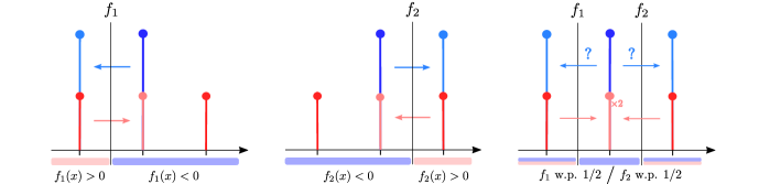
Consider the binary classification task illustrated in Figure 1. We assume that all input-output pairs (X,Y)(X,Y) are sampled from a distribution \mathbb{P} defined as follows

(Y=±1)=1/2 and {(X=0Y=1)=1(X=±1Y=1)=1/2\mathbb{P}\left(Y=\pm 1\right)=1/2\ \mbox{ and }\left\{\begin{array}[]{ll}\mathbb{P}\left(X=0\mid Y=-1\right)=1\\ \mathbb{P}\left(X=\pm 1\mid Y=1\right)=1/2\end{array}\right.

Given access to \mathbb{P}, the adversary aims to maximize the expected risk, but can only move each point by at most 11 on the real line. In this context, we study two classifiers: f1(x)=x1/2f_{1}(x)=-x-1/2 and f2(x)=x1/2f_{2}(x)=x-1/2111(X,Y)(X,Y)\sim\mathbb{P} is misclassified by fif_{i} if and only if fi(X)Y0f_{i}(X)Y\leq 0. Both f1f_{1} and f2f_{2} have a standard risk of 1/41/4. In the presence of an adversary, the risk (a.k.a. the adversarial risk) increases to 11. Here, using a randomized classifier can make the system more robust. Consider ff where f=f1f=f_{1} w.p. 1/21/2 and f2f_{2} otherwise. The standard risk of ff remains 1/41/4 but its adversarial risk is 3/4<13/4<1. Indeed, when attacking ff, any adversary will have to choose between moving points from 0 to 11 or to 1-1. Either way, the attack only works half of the time; hence an overall adversarial risk of 3/43/4. Furthermore, if ff knows the strategy the adversary uses, it can always update the probability it gives to f1f_{1} and f2f_{2} to get a better (possibly deterministic) defense. For example, if the adversary chooses to always move 0 to 11, the classifier can set f=f1f=f_{1} w.p. 11 to retrieve an adversarial risk of 1/21/2 instead of 3/43/4.

Now, what happens if the adversary can use randomized strategies, meaning that for each point it can flip a coin before deciding where to move? In this case, the adversary could decide to move points from 0 to 11 w.p. 1/21/2 and to 1-1 otherwise. This strategy is still optimal with an adversarial risk of 3/43/4 but now the classifier cannot use its knowledge of the adversary’s strategy to lower the risk. We are in a state where neither the adversary nor the classifier can benefit from unilaterally changing its strategy. In the game theory terminology, this state is called a Mixed Nash equilibrium.

2.2 General setting

Let us consider a classification task with input space 𝒳\mathcal{X} and output space 𝒴\mathcal{Y}. Let (𝒳,d)(\mathcal{X},d) be a proper (i.e. closed balls are compact) Polish (i.e. completely separable) metric space representing the inputs space222For instance, for any norm \lVert\cdot\rVert, (d,)(\mathbb{R}^{d},\lVert\cdot\rVert) is a proper Polish metric space.. Let 𝒴={1,,K}\mathcal{Y}=\{1,\dots,K\} be the labels set, endowed with the trivial metric d(y,y)=𝟏yyd^{\prime}(y,y^{\prime})=\mathbf{1}_{y\neq y^{\prime}}. Then the space (𝒳×𝒴,dd)(\mathcal{X}\times\mathcal{Y},d\oplus d^{\prime}) is a proper Polish space. For any Polish space 𝒵\mathcal{Z}, we denote +1(𝒵)\mathcal{M}_{+}^{1}(\mathcal{Z}) the Polish space of Borel probability measures on 𝒵\mathcal{Z}. Let us assume the data is drawn from +1(𝒳×𝒴)\mathbb{P}\in\mathcal{M}_{+}^{1}(\mathcal{X}\times\mathcal{Y}). Let (Θ,dΘ)(\Theta,d_{\Theta}) be a Polish space (not necessarily proper) representing the set of classifier parameters (for instance neural networks). We also define a loss function: l:Θ×(𝒳×𝒴)[0,)l:\Theta\times(\mathcal{X}\times\mathcal{Y})\to[0,\infty) satisfying the following set of assumptions.

Assumption 1 (Loss function).

1) The loss function ll is a non negative Borel measurable function. 2) For all θΘ\theta\in\Theta, l(θ,)l(\theta,\cdot) is upper-semi continuous. 3) There exists M>0M>0 such that for all θΘ\theta\in\Theta, (x,y)𝒳×𝒴(x,y)\in\mathcal{X}\times\mathcal{Y}, 0l(θ,(x,y))M0\leq l(\theta,(x,y))\leq M.

It is usual to assume upper-semi continuity when studying optimization over distributions [38, 7]. Furthermore, considering bounded (and positive) loss functions is also very common in learning theory [2] and is not restrictive.

In the adversarial examples framework, the loss of interest is the 0/10/1 loss, for whose surrogates are misunderstood [14, 1]; hence it is essential that the 0/10/1 loss satisfies Assumption 1. In the binary classification setting (i.e. 𝒴={1,+1}\mathcal{Y}=\{-1,+1\}) the 0/10/1 loss writes l0/1(θ,(x,y))=𝟏yfθ(x)0l_{0/1}(\theta,(x,y))=\mathbf{1}_{yf_{\theta}(x)\leq 0}. Then, assuming that for all θ\theta, fθ()f_{\theta}(\cdot) is continuous and for all xx, f(x)f_{\cdot}(x) is continuous, the 0/10/1 loss satisfies Assumption 1. In particular, it is the case for neural networks with continuous activation functions.

2.3 Adversarial Risk Minimization

The standard risk for a single classifier θ\theta associated with the loss ll satisfying Assumption 1 writes: (θ):=𝔼(x,y)[l(θ,(x,y))]\mathcal{R}(\theta):=\mathbb{E}_{(x,y)\sim\mathbb{P}}\left[l(\theta,(x,y))\right]. Similarly, the adversarial risk of θ\theta at level ε\varepsilon associated with the loss ll is defined as333For the well-posedness, see Lemma 4 in Appendix.

advε(θ):=𝔼(x,y)[supx𝒳,d(x,x)εl(θ,(x,y))].\displaystyle\mathcal{R}_{adv}^{\varepsilon}(\theta):=\mathbb{E}_{(x,y)\sim\mathbb{P}}\left[\sup_{x^{\prime}\in\mathcal{X},~{}d(x,x^{\prime})\leq\varepsilon}l(\theta,(x^{\prime},y))\right].

It is clear that adv0(θ)=(θ)\mathcal{R}_{adv}^{0}(\theta)=\mathcal{R}(\theta) for all θ\theta. We can generalize these notions with distributions of classifiers. In other terms the classifier is then randomized according to some distribution μ+1(Θ)\mu\in\mathcal{M}^{1}_{+}(\Theta). A classifier is randomized if for a given input, the output of the classifier is a probability distribution. The standard risk of a randomized classifier μ\mu writes (μ)=𝔼θμ[(θ)]\mathcal{R}(\mu)=\mathbb{E}_{\theta\sim\mu}\left[\mathcal{R}(\theta)\right]. Similarly, the adversarial risk of the randomized classifier μ\mu at level ε\varepsilon is444This risk is also well posed (see Lemma 4 in the Appendix).

advε(μ):=𝔼(x,y)[supx𝒳,d(x,x)ε𝔼θμ[l(θ,(x,y))]].\displaystyle\mathcal{R}_{adv}^{\varepsilon}(\mu):=\mathbb{E}_{(x,y)\sim\mathbb{P}}\left[\sup_{x^{\prime}\in\mathcal{X},~{}d(x,x^{\prime})\leq\varepsilon}\mathbb{E}_{\theta\sim\mu}\left[l(\theta,(x^{\prime},y))\right]\right].

For instance, for the 0/10/1 loss, the inner maximization problem, consists in maximizing the probability of misclassification for a given couple (x,y)(x,y). Note that (δθ)=(θ)\mathcal{R}(\delta_{\theta})=\mathcal{R}(\theta) and advε(δθ)=advε(θ)\mathcal{R}_{adv}^{\varepsilon}(\delta_{\theta})=\mathcal{R}_{adv}^{\varepsilon}(\theta). In the remainder of the paper, we study the adversarial risk minimization problems with randomized and deterministic classifiers and denote

𝒱randε:=infμ+1(Θ)advε(μ),𝒱detε:=infθΘadvε(θ)\displaystyle\mathcal{V}_{rand}^{\varepsilon}:=\inf_{\mu\in\mathcal{M}^{1}_{+}(\Theta)}\mathcal{R}_{adv}^{\varepsilon}(\mu),~{}\mathcal{V}_{det}^{\varepsilon}:=\inf_{\theta\in\Theta}\mathcal{R}_{adv}^{\varepsilon}(\theta) (1)
Remark 1.

We can show (see Appendix E) that the standard risk infima are equal : 𝒱rand0=𝒱det0\mathcal{V}_{rand}^{0}=\mathcal{V}_{det}^{0}. Hence, no randomization is needed for minimizing the standard risk. Denoting 𝒱\mathcal{V} this common value, we also have the following inequalities for any ε>0\varepsilon>0, 𝒱𝒱randε𝒱detε\mathcal{V}\leq\mathcal{V}_{rand}^{\varepsilon}\leq\mathcal{V}_{det}^{\varepsilon}.

2.4 Distributional Formulation of the Adversarial Risk

To account for the possible randomness of the adversary, we rewrite the adversarial attack problem as a convex optimization problem on distributions. Let us first introduce the set of adversarial distributions.

Definition 1 (Set of adversarial distributions).

Let \mathbb{P} be a Borel probability distribution on 𝒳×𝒴\mathcal{X}\times\mathcal{Y} and ε>0\varepsilon>0. We define the set of adversarial distributions as

𝒜ε\displaystyle\mathcal{A}_{\varepsilon} ():={1+(𝒳×𝒴)γ1+((𝒳×𝒴)2),\displaystyle(\mathbb{P}):=\left\{\mathbb{Q}\in\mathcal{M}^{+}_{1}(\mathcal{X}\times\mathcal{Y})\mid\exists\gamma\in\mathcal{M}^{+}_{1}\left((\mathcal{X}\times\mathcal{Y})^{2}\right),\right.
d(x,x)ε,y=yγ-a.s.,Π1γ=,Π2γ=}\displaystyle\left.d(x,x^{\prime})\leq\varepsilon,~{}y=y^{\prime}~{}~{}\gamma\text{-a.s.},~{}\Pi_{1\sharp}\gamma=\mathbb{P},~{}\Pi_{2\sharp}\gamma=\mathbb{Q}\right\}

where Πi\Pi_{i} denotes the projection on the ii-th component, and gg_{\sharp} the push-forward measure by a measurable function gg.

For an attacker that can move the initial distribution \mathbb{P} in 𝒜ε()\mathcal{A}_{\varepsilon}(\mathbb{P}), the attack would not be a transport map as considered in the standard adversarial risk. For every point xx in the support of \mathbb{P}, the attacker is allowed to move xx randomly in the ball of radius ε\varepsilon, and not to a single other point xx^{\prime} like the usual attacker in adversarial attacks. In this sense, we say the attacker is allowed to be randomized.

Link with DRO. Adversarial examples have been studied in the light of DRO by former works [33, 37], but an exact reformulation of the adversarial risk as a DRO problem has not been made yet. When (𝒵,d)(\mathcal{Z},d) is a Polish space and c:𝒵2+{+}c:\mathcal{Z}^{2}\rightarrow\mathbb{R}^{+}\cup\{+\infty\} is a lower semi-continuous function, for ,1+(𝒵)\mathbb{P},\mathbb{Q}\in\mathcal{M}^{+}_{1}(\mathcal{Z}) , the primal Optimal Transport problem is defined as

Wc(,):=infγΓ,𝒵2c(z,z)𝑑γ(z,z)\displaystyle W_{c}(\mathbb{P},\mathbb{Q}):=\inf_{\gamma\in\Gamma_{\mathbb{P},\mathbb{Q}}}\int_{\mathcal{Z}^{2}}c(z,z^{\prime})d\gamma(z,z^{\prime})

with Γ,:={γ1+(𝒵2)Π1γ=,Π2γ=}\Gamma_{\mathbb{P},\mathbb{Q}}:=\left\{\gamma\in\mathcal{M}^{+}_{1}(\mathcal{Z}^{2})\mid~{}\Pi_{1\sharp}\gamma=\mathbb{P},~{}\Pi_{2\sharp}\gamma=\mathbb{Q}\right\}. When η>0\eta>0 and for 1+(𝒵)\mathbb{P}\in\mathcal{M}^{+}_{1}(\mathcal{Z}), the associated Wasserstein uncertainty set is defined as:

c(,η):={1+(𝒵)Wc(,)η}\displaystyle\mathcal{B}_{c}(\mathbb{P},\eta):=\left\{\mathbb{Q}\in\mathcal{M}^{+}_{1}(\mathcal{Z})\mid W_{c}(\mathbb{P},\mathbb{Q})\leq\eta\right\}

A DRO problem is a linear optimization problem over Wasserstein uncertainty sets supc(,η)g(z)𝑑(z)\sup_{\mathbb{Q}\in\mathcal{B}_{c}(\mathbb{P},\eta)}\int g(z)d\mathbb{Q}(z) for some upper semi-continuous function gg [41]. For an arbitrary ε>0\varepsilon>0, we define the cost cεc_{\varepsilon} as follows

cε((x,y),(x,y)):={0if d(x,x)ε and y=y+otherwise.\displaystyle c_{\varepsilon}((x,y),(x^{\prime},y^{\prime})):=\left\{\begin{array}[]{ll}0&\mbox{if }d(x,x^{\prime})\leq\varepsilon\mbox{ and }y=y^{\prime}\\ +\infty&\mbox{otherwise.}\end{array}\right.

This cost is lower semi-continuous and penalizes to infinity perturbations that change the label or move the input by a distance greater than ε\varepsilon. As Proposition 1 shows, the Wasserstein ball associated with cεc_{\varepsilon} is equal to 𝒜ε()\mathcal{A}_{\varepsilon}(\mathbb{P}).

Proposition 1.

Let \mathbb{P} be a Borel probability distribution on 𝒳×𝒴\mathcal{X}\times\mathcal{Y} and ε>0\varepsilon>0 and η0\eta\geq 0, then cε(,η)=𝒜ε()\mathcal{B}_{c_{\varepsilon}}(\mathbb{P},\eta)=\mathcal{A}_{\varepsilon}(\mathbb{P}). Moreover, 𝒜ε()\mathcal{A}_{\varepsilon}(\mathbb{P}) is convex and compact for the weak topology of 1+(𝒳×𝒴)\mathcal{M}^{+}_{1}(\mathcal{X}\times\mathcal{Y}).

Thanks to this result, we can reformulate the adversarial risk as the value of a convex problem over 𝒜ε()\mathcal{A}_{\varepsilon}(\mathbb{P}).

Proposition 2.

Let \mathbb{P} be a Borel probability distribution on 𝒳×𝒴\mathcal{X}\times\mathcal{Y} and μ\mu a Borel probability distribution on Θ\Theta. Let l:Θ×(𝒳×𝒴)[0,)l:\Theta\times(\mathcal{X}\times\mathcal{Y})\to[0,\infty) satisfying Assumption 1. Let ε>0\varepsilon>0. Then:

advε(μ)=sup𝒜ε()𝔼(x,y),θμ[l(θ,(x,y))].\displaystyle\mathcal{R}_{adv}^{\varepsilon}(\mu)=\sup_{\mathbb{Q}\in\mathcal{A}_{\varepsilon}(\mathbb{P})}\mathbb{E}_{(x^{\prime},y^{\prime})\sim\mathbb{Q},\theta\sim\mu}\left[l(\theta,(x^{\prime},y^{\prime}))\right]. (2)

The supremum is attained. Moreover 𝒜ε()\mathbb{Q}^{*}\in\mathcal{A}_{\varepsilon}(\mathbb{P}) is an optimum of Problem (2) if and only if there exists γ1+((𝒳×𝒴)2)\gamma^{*}\in\mathcal{M}^{+}_{1}\left((\mathcal{X}\times\mathcal{Y})^{2}\right) such that: Π1γ=\Pi_{1\sharp}\gamma^{*}=\mathbb{P}, Π2γ=\Pi_{2\sharp}\gamma^{*}=\mathbb{Q}^{*}, d(x,x)εd(x,x^{\prime})\leq\varepsilon, y=yy=y^{\prime} and l(x,y)=supu𝒳,d(x,u)εl(u,y)l(x^{\prime},y^{\prime})=\sup_{\begin{subarray}{c}u\in\mathcal{X},d(x,u)\leq\varepsilon\end{subarray}}l(u,y) γ\gamma^{*}-almost surely.

The adversarial attack problem is a DRO problem for the cost cεc_{\varepsilon}. Proposition 2 means that, against a fixed classifier μ\mu, the randomized attacker that can move the distribution in 𝒜ε()\mathcal{A}_{\varepsilon}(\mathbb{P}) has exactly the same power as an attacker that moves every single point xx in the ball of radius ε\varepsilon. By Proposition 2, we also deduce that the adversarial risk can be casted as a linear optimization problem over distributions.

Remark 2.

In a recent work, [29] proposed a similar adversary using Markov kernels but left as an open question the link with the classical adversarial risk, due to measurability issues. Proposition 2 solves these issues. The result is similar to [7]. Although we believe its proof might be extended for infinite valued costs, [7] did not treat that case. We provide an alternative proof in this special case.

3 Nash Equilibria in the Adversarial Game

3.1 Adversarial Attacks as a Zero-Sum Game

Thanks to Proposition 2, the adversarial risk minimization problem can be seen as a two-player zero-sum game that writes as follows,

infμ+1(Θ)sup𝒜ε()𝔼(x,y),θμ[l(θ,(x,y))].\displaystyle\inf_{\mu\in\mathcal{M}^{1}_{+}(\Theta)}\sup_{\mathbb{Q}\in\mathcal{A}_{\varepsilon}(\mathbb{P})}\mathbb{E}_{(x,y)\sim\mathbb{Q},\theta\sim\mu}\left[l(\theta,(x,y))\right]. (3)

In this game the classifier objective is to find the best distribution μ1+(Θ)\mu\in\mathcal{M}_{1}^{+}(\Theta) while the adversary is manipulating the data distribution. For the classifier, solving the infimum problem in Equation (3) simply amounts to solving the adversarial risk minimization problem – Problem (1), whether the classifier is randomized or not. Then, given a randomized classifier μ1+(Θ)\mu\in\mathcal{M}_{1}^{+}(\Theta), the goal of the attacker is to find a new data-set distribution \mathbb{Q} in the set of adversarial distributions 𝒜ε()\mathcal{A}_{\varepsilon}(\mathbb{P}) that maximizes the risk of μ\mu. More formally, the adversary looks for

argmax𝒜ε()𝔼(x,y),θμ[l(θ,(x,y))].\mathbb{Q}\in\operatorname*{argmax}_{\mathbb{Q}\in\mathcal{A}_{\varepsilon}(\mathbb{P})}\mathbb{E}_{(x,y)\sim\mathbb{Q},\theta\sim\mu}\left[l(\theta,(x,y))\right].

In the game theoretic terminology, \mathbb{Q} is also called the best response of the attacker to the classifier θ\theta.

Remark 3.

Note that for a given classifier μ\mu there always exists a “deterministic” best response, i.e. every single point xx is mapped to another single point T(x)T(x). Let T:𝒳𝒳T:\mathcal{X}\to\mathcal{X} be defined such that for all x𝒳x\in\mathcal{X}, l(T(x),y)=supx,d(x,x)εl(x,y)l(T(x),y)=\sup_{x^{\prime},~{}d(x,x^{\prime})\leq\varepsilon}l(x^{\prime},y). Thanks to [4, Proposition 7.50], (T,id)(T,id) is \mathbb{P}-measurable. Then (T,id)(T,id)_{\sharp}\mathbb{P} belongs to BR(μ)\text{BR}(\mu). Therefore, TT is the optimal “deterministic” attack against the classifier μ\mu.

3.2 Dual Formulation of the Game

Every zero sum game has a dual formulation that allows for a deeper understanding of the framework. Here, from Proposition 2, we can define the dual problem of adversarial risk minimization for randomized classifiers. This dual problem also characterizes a two-player zero-sum game that writes as follows,

sup𝒜ε()infμ+1(Θ)𝔼(x,y),θμ[l(θ,(x,y))].\displaystyle\sup_{\mathbb{Q}\in\mathcal{A}_{\varepsilon}(\mathbb{P})}\inf_{\mu\in\mathcal{M}^{1}_{+}(\Theta)}\mathbb{E}_{(x,y)\sim\mathbb{Q},\theta\sim\mu}\left[l(\theta,(x,y))\right]. (4)

In this dual game problem, the adversary plays first and seeks an adversarial distribution that has the highest possible risk when faced with an arbitrary classifier. This means that it has to select an adversarial perturbation for every input xx, without seeing the classifier first. In this case, as pointed out by the motivating example in Section 2.1, the attack can (and should) be randomized to ensure maximal harm against several classifiers. Then, given an adversarial distribution, the classifier objective is to find the best possible classifier on this distribution. Let us denote 𝒟ε\mathcal{D}^{\varepsilon} the value of the dual problem. Since the weak duality is always satisfied, we get

𝒟ε𝒱randε𝒱detε.\displaystyle\mathcal{D}^{\varepsilon}\leq\mathcal{V}_{rand}^{\varepsilon}\leq\mathcal{V}_{det}^{\varepsilon}. (5)

Inequalities in Equation (5) mean that the lowest risk the classifier can get (regardless of the game we look at) is 𝒟ε\mathcal{D}^{\varepsilon}. In particular, this means that the primal version of the game, i.e. the adversarial risk minimization problem, will always have a value greater or equal to 𝒟ε\mathcal{D}^{\varepsilon}. As we discussed in Section 2.1, this lower bound may not be attained by a deterministic classifier. As we will demonstrate in the next section, optimizing over randomized classifiers allows to approach 𝒟ε\mathcal{D}^{\varepsilon} arbitrary closely.

Remark 4.

Note that, we can always define the dual problem when the classifier is deterministic,

sup𝒜ε()infθΘ𝔼(x,y)[l(θ,(x,y))].\displaystyle\sup_{\mathbb{Q}\in\mathcal{A}_{\varepsilon}(\mathbb{P})}\inf_{\theta\in\Theta}\mathbb{E}_{(x,y)\sim\mathbb{Q}}\left[l(\theta,(x,y))\right].

Furthermore, we can demonstrate that the dual problems for deterministic and randomized classifiers have the same value 555See Appendix E for more details; hence the inequalities in Equation (5).

3.3 Nash Equilibria for Randomized Strategies

In the adversarial examples game, a Nash equilibrium is a couple (μ,)+1(Θ)×𝒜ε()(\mu^{*},\mathbb{Q}^{*})\in\mathcal{M}^{1}_{+}(\Theta)\times\mathcal{A}_{\varepsilon}(\mathbb{P}) where both the classifier and the attacker have no incentive to deviate unilaterally from their strategies μ\mu^{*} and \mathbb{Q}^{*}. More formally, (μ,)(\mu^{*},\mathbb{Q}^{*}) is a Nash equilibrium of the adversarial examples game if (μ,)(\mu^{*},\mathbb{Q}^{*}) is a saddle point of the objective function

(μ,)𝔼(x,y),θμ[l(θ,(x,y))].(\mu,\mathbb{Q})\mapsto\mathbb{E}_{(x,y)\sim\mathbb{Q},\theta\sim\mu}\left[l(\theta,(x,y))\right].

Alternatively, we can say that (μ,)(\mu^{*},\mathbb{Q}^{*}) is a Nash equilibrium if and only if μ\mu^{*} solves the adversarial risk minimization problem – Problem (1), \mathbb{Q}^{*} the dual problem – Problem (6), and 𝒟ε=𝒱randε\mathcal{D}^{\varepsilon}=\mathcal{V}_{rand}^{\varepsilon}. In our problem, \mathbb{Q}^{*} always exists but it might not be the case for μ\mu^{*}. Then for any δ>0\delta>0, we say that (μδ,)(\mu_{\delta},\mathbb{Q}^{*}) is a δ\delta-approximate Nash equilibrium if \mathbb{Q}^{*} solves the dual problem and μδ\mu_{\delta} satisfies 𝒟εadvε(μδ)δ\mathcal{D}^{\varepsilon}\geq\mathcal{R}_{adv}^{\varepsilon}(\mu_{\delta})-\delta.

We now state our main result: the existence of approximate Nash equilibria in the adversarial examples game when both the classifier and the adversary can use randomized strategies. More precisely, we demonstrate that the duality gap between the adversary and the classifier problems is zero, which gives as a corollary the existence of Nash equilibria.

Theorem 1.

Let +1(𝒳×𝒴)\mathbb{P}\in\mathcal{M}^{1}_{+}(\mathcal{X}\times\mathcal{Y}). Let ε>0\varepsilon>0. Let l:Θ×(𝒳×𝒴)[0,)l:\Theta\times(\mathcal{X}\times\mathcal{Y})\to[0,\infty) satisfying Assumption 1. Then strong duality always holds in the randomized setting:

infμ1+(Θ)max𝒜ε()𝔼θμ,(x,y)[l(θ,(x,y))]\displaystyle\inf_{\mu\in\mathcal{M}^{+}_{1}(\Theta)}\max_{\mathbb{Q}\in\mathcal{A}_{\varepsilon}(\mathbb{P})}\mathbb{E}_{\theta\sim\mu,(x,y)\sim\mathbb{Q}}\left[l(\theta,(x,y))\right] (6)
=max𝒜ε()infμ1+(Θ)𝔼θμ,(x,y)[l(θ,(x,y))]\displaystyle=\max_{\mathbb{Q}\in\mathcal{A}_{\varepsilon}(\mathbb{P})}\inf_{\mu\in\mathcal{M}^{+}_{1}(\Theta)}\mathbb{E}_{\theta\sim\mu,(x,y)\sim\mathbb{Q}}\left[l(\theta,(x,y))\right]

The supremum is always attained. If Θ\Theta is a compact set, and for all (x,y)𝒳×𝒴(x,y)\in\mathcal{X}\times\mathcal{Y}, l(,(x,y))l(\cdot,(x,y)) is lower semi-continuous, the infimum is also attained.

Corollary 1.

Under Assumption 1, for any δ>0\delta>0, there exists a δ\delta-approximate Nash-Equibilrium (μδ,)(\mu_{\delta},\mathbb{Q}^{*}). Moreover, if the infimum is attained, there exists a Nash equilibrium (μ,)(\mu^{*},\mathbb{Q}^{*}) to the adversarial examples game.

Theorem 1 shows that 𝒟ε=𝒱randε\mathcal{D}^{\varepsilon}=\mathcal{V}_{rand}^{\varepsilon}. From a game theoretic perspective, this means that the minimal adversarial risk for a randomized classifier against any attack (primal problem) is the same as the maximal risk an adversary can get by using an attack strategy that is oblivious to the classifier it faces (dual problem). This suggests that playing randomized strategies for the classifier could substantially improve robustness to adversarial examples. In the next section, we will design an algorithm that efficiently learn this classifier, we will get improve adversarial robustness over classical deterministic defenses.

Remark 5.

Theorem 1 remains true if one replaces 𝒜ε()\mathcal{A}_{\varepsilon}(\mathbb{P}) with any other Wasserstein compact uncertainty sets (see [41] for conditions of compactness).

4 Finding the Optimal Classifiers

4.1 An Entropic Regularization

Let {(xi,yi)}i=1N\{(x_{i},y_{i})\}_{i=1}^{N} samples independently drawn from \mathbb{P} and denote ^:=1Ni=1Nδ(xi,yi)\widehat{\mathbb{P}}:=\frac{1}{N}\sum_{i=1}^{N}\delta_{(x_{i},y_{i})} the associated empirical distribution. One can show the adversarial empirical risk minimization can be casted as:

^advε,:=infμ1+(Θ)i=1NsupiΓi,ε𝔼(x,y)i,θμ[l(θ,(x,y))]\displaystyle\widehat{\mathcal{R}}_{adv}^{\varepsilon,*}:=\inf_{\mu\in\mathcal{M}^{+}_{1}(\Theta)}\sum_{i=1}^{N}\sup_{\mathbb{Q}_{i}\in\Gamma_{i,\varepsilon}}\mathbb{E}_{(x,y)\sim\mathbb{Q}_{i},\theta\sim\mu}\left[l(\theta,(x,y))\right]

where Γi,ε\Gamma_{i,\varepsilon} is defined as :

Γi,ε:={i𝑑i=1N,cε((xi,yi),)𝑑i=0}.\displaystyle\Gamma_{i,\varepsilon}:=\Big{\{}\mathbb{Q}_{i}\mid~{}\int d\mathbb{Q}_{i}=\frac{1}{N},~{}\int c_{\varepsilon}((x_{i},y_{i}),\cdot)d\mathbb{Q}_{i}=0\Big{\}}.

More details on this decomposition are given in Appendix E. In the following, we regularize the above objective by adding an entropic term to each inner supremum problem. Let 𝜶:=(αi)i=1N+N\bm{\alpha}:=(\alpha_{i})_{i=1}^{N}\in\mathbb{R}_{+}^{N} such that for all i{1,,N}i\in\{1,\dots,N\}, and let us consider the following optimization problem:

^adv,𝜶ε,:=infμ1+(Θ)i=1N\displaystyle\widehat{\mathcal{R}}_{adv,\bm{\alpha}}^{\varepsilon,*}:=\inf_{\mu\in\mathcal{M}^{+}_{1}(\Theta)}\sum_{i=1}^{N} supiΓi,ε𝔼i,μ[l(θ,(x,y))]\displaystyle\sup_{\mathbb{Q}_{i}\in\Gamma_{i,\varepsilon}}\mathbb{E}_{\mathbb{Q}_{i},\mu}\left[l(\theta,(x,y))\right]
αiKL(i||1N𝕌(xi,yi))\displaystyle-\alpha_{i}\text{KL}\left(\mathbb{Q}_{i}\Big{|}\Big{|}\frac{1}{N}\mathbb{U}_{(x_{i},y_{i})}\right)

where 𝕌(x,y)\mathbb{U}_{(x,y)} is an arbitrary distribution of support equal to:

S(x,y)(ε):={(x,y):s.t.cε((x,y),(x,y))=0},\displaystyle S_{(x,y)}^{(\varepsilon)}:=\Big{\{}(x^{\prime},y^{\prime}):~{}\text{s.t.}~{}c_{\varepsilon}((x,y),(x^{\prime},y^{\prime}))=0\Big{\}},

and for all ,𝕌+(𝒳×𝒴)\mathbb{Q},\mathbb{U}\in\mathcal{M}_{+}(\mathcal{X}\times\mathcal{Y}),

KL(||𝕌):={log(dd𝕌)𝑑+|𝕌|||if 𝕌+otherwise.\displaystyle\text{KL}(\mathbb{Q}||\mathbb{U}):=\left\{\begin{array}[]{lll}\int\log(\frac{d\mathbb{Q}}{d\mathbb{U}})d\mathbb{Q}+|\mathbb{U}|-|\mathbb{Q}|&\mbox{if }\mathbb{Q}\ll\mathbb{U}\\ +\infty&\mbox{otherwise.}\end{array}\right.

Note that when 𝜶=0\bm{\alpha}=0, we recover the problem of interest ^adv,𝜶ε,=^advε,\widehat{\mathcal{R}}_{adv,\bm{\alpha}}^{\varepsilon,*}=\widehat{\mathcal{R}}_{adv}^{\varepsilon,*}. Moreover, we show the regularized supremum tends to the standard supremum when 𝜶0\bm{\alpha}\to 0.

Proposition 3.

For μ1+(Θ)\mu\in\mathcal{M}_{1}^{+}(\Theta), one has

limαi0supiΓi,ε𝔼i,μ[l(θ,(x,y))]αiKL(||1N𝕌(xi,yi))\displaystyle\lim_{\alpha_{i}\rightarrow 0}\sup_{\mathbb{Q}_{i}\in\Gamma_{i,\varepsilon}}\mathbb{E}_{\mathbb{Q}_{i},\mu}\left[l(\theta,(x,y))\right]-\alpha_{i}\text{KL}\left(\mathbb{Q}\Big{|}\Big{|}\frac{1}{N}\mathbb{U}_{(x_{i},y_{i})}\right)
=supiΓi,ε𝔼(x,y)i,θμ[l(θ,(x,y))].\displaystyle=\sup_{\mathbb{Q}_{i}\in\Gamma_{i,\varepsilon}}\mathbb{E}_{(x,y)\sim\mathbb{Q}_{i},\theta\sim\mu}\left[l(\theta,(x,y))\right].

By adding an entropic term to the objective, we obtain an explicit formulation of the supremum involved in the sum: as soon as 𝜶>0\bm{\alpha}>0 (which means that each αi>0\alpha_{i}>0), each sub-problem becomes just the Fenchel-Legendre transform of KL(|𝕌(xi,yi)/N)\text{KL}(\cdot|\mathbb{U}_{(x_{i},y_{i})}/N) which has the following closed form:

supiΓi,ε𝔼i,μ[l(θ,(x,y))]αiKL(i||1N𝕌(xi,yi))\displaystyle\sup_{\mathbb{Q}_{i}\in\Gamma_{i,\varepsilon}}\mathbb{E}_{\mathbb{Q}_{i},\mu}\left[l(\theta,(x,y))\right]-\alpha_{i}\text{KL}\left(\mathbb{Q}_{i}||\frac{1}{N}\mathbb{U}_{(x_{i},y_{i})}\right)
=αiNlog(𝒳×𝒴exp(𝔼θμ[l(θ,(x,y))]αi)𝑑𝕌(xi,yi)).\displaystyle=\frac{\alpha_{i}}{N}\log\left(\int_{\mathcal{X}\times\mathcal{Y}}\exp\left(\frac{\mathbb{E}_{\theta\sim\mu}\left[l(\theta,(x,y))\right]}{\alpha_{i}}\right)d\mathbb{U}_{(x_{i},y_{i})}\right).

Finally, we end up with the following problem:

infμ1+(Θ)i=1NαiNlog(exp𝔼μ[l(θ,(x,y))]αid𝕌(xi,yi)).\displaystyle\inf_{\mu\in\mathcal{M}^{+}_{1}(\Theta)}\sum_{i=1}^{N}\frac{\alpha_{i}}{N}\log\left(\int\exp\frac{\mathbb{E}_{\mu}\left[l(\theta,(x,y))\right]}{\alpha_{i}}d\mathbb{U}_{(x_{i},y_{i})}\right).

In order to solve the above problem, one needs to compute the integral involved in the objective. To do so, we estimate it by randomly sampling mi1m_{i}\geq 1 samples (u1(i),,umi(i))(𝒳×𝒴)mi(u_{1}^{(i)},\dots,u_{m_{i}}^{(i)})\in(\mathcal{X}\times\mathcal{Y})^{m_{i}} from 𝕌(xi,yi)\mathbb{U}_{(x_{i},y_{i})} for all i{1,,N}i\in\{1,\dots,N\} which leads to the following optimization problem

infμ1+(Θ)i=1NαiNlog(1mij=1miexp𝔼μ[l(θ,uj(i))]αi)\displaystyle\inf_{\mu\in\mathcal{M}^{+}_{1}(\Theta)}\sum_{i=1}^{N}\frac{\alpha_{i}}{N}\log\left(\frac{1}{m_{i}}\sum_{j=1}^{m_{i}}\exp\frac{\mathbb{E}_{\mu}\left[l(\theta,u_{j}^{(i)})\right]}{\alpha_{i}}\right) (7)

denoted ^adv,𝜶ε,𝒎\widehat{\mathcal{R}}_{adv,\bm{\alpha}}^{\varepsilon,\bm{m}} where 𝒎:=(mi)i=1N\bm{m}:=(m_{i})_{i=1}^{N} in the following. Now we aim at controlling the error made with our approximations. We decompose the error into two terms

|^adv,𝜶ε,𝒎^advε,||^adv,𝜶ε,^adv,𝜶ε,𝒎|+|^adv,𝜶ε,^advε,|\displaystyle|\widehat{\mathcal{R}}_{adv,\bm{\alpha}}^{\varepsilon,\bm{m}}-\widehat{\mathcal{R}}_{adv}^{\varepsilon,*}|\leq|\widehat{\mathcal{R}}_{adv,\bm{\alpha}}^{\varepsilon,*}-\widehat{\mathcal{R}}_{adv,\bm{\alpha}}^{\varepsilon,\bm{m}}|+|\widehat{\mathcal{R}}_{adv,\bm{\alpha}}^{\varepsilon,*}-\widehat{\mathcal{R}}_{adv}^{\varepsilon,*}|

where the first one corresponds to the statistical error made by our estimation of the integral, and the second to the approximation error made by the entropic regularization of the objective. First, we show a control of the statistical error using Rademacher complexities [2].

Proposition 4.

Let m1m\geq 1 and α>0\alpha>0 and denote 𝛂:=(α,,α)N\bm{\alpha}:=(\alpha,\dots,\alpha)\in\mathbb{R}^{N} and 𝐦:=(m,,m)N\bm{m}:=(m,\dots,m)\in\mathbb{R}^{N}. Then by denoting M~=max(M,1)\tilde{M}=\max(M,1), we have with a probability of at least 1δ1-\delta

|^adv,𝜶ε,^adv,𝜶ε,𝒎|\displaystyle|\widehat{\mathcal{R}}_{adv,\bm{\alpha}}^{\varepsilon,*}-\widehat{\mathcal{R}}_{adv,\bm{\alpha}}^{\varepsilon,\bm{m}}|\leq 2eM/αNi=1NRi+6M~eM/αlog(4δ)2mN\displaystyle\frac{2e^{M/\alpha}}{N}\sum_{i=1}^{N}R_{i}+\color[rgb]{0,0,0}\definecolor[named]{pgfstrokecolor}{rgb}{0,0,0}\pgfsys@color@gray@stroke{0}\pgfsys@color@gray@fill{0}{6\tilde{M}}\color[rgb]{0,0,0}\definecolor[named]{pgfstrokecolor}{rgb}{0,0,0}\pgfsys@color@gray@stroke{0}\pgfsys@color@gray@fill{0}e^{M/\alpha}\sqrt{\frac{\log(\frac{4}{\delta})}{2mN}}

where Ri:=1m𝔼𝛔[supθΘj=1mσjl(θ,uj(i))]R_{i}:=\frac{1}{m}\mathbb{E}_{\bm{\sigma}}\left[\sup_{\theta\in\Theta}\sum_{j=1}^{m}\sigma_{j}l(\theta,u_{j}^{(i)})\right] and 𝛔:=(σ1,,σm)\bm{\sigma}:=(\sigma_{1},\dots,\sigma_{m}) with σi\sigma_{i} i.i.d. sampled as [σi=±1]=1/2\mathbb{P}[\sigma_{i}=\pm 1]=1/2.

We deduce from the above Proposition that in the particular case where Θ\Theta is finite such that |Θ|=L|\Theta|=L, with probability of at least 1δ1-\delta

|^adv,𝜶ε,^adv,𝜶ε,𝒎|𝒪(MeM/αlog(L)m).\displaystyle|\widehat{\mathcal{R}}_{adv,\bm{\alpha}}^{\varepsilon,*}-\widehat{\mathcal{R}}_{adv,\bm{\alpha}}^{\varepsilon,\bm{m}}|\in\mathcal{O}\left(Me^{M/\alpha}\sqrt{\frac{\log(L)}{m}}\right).

This case is of particular interest when one wants to learn the optimal mixture of some given classifiers in order to minimize the adversarial risk. In the following proposition, we control the approximation error made by adding an entropic term to the objective.

Proposition 5.

Denote for β>0\beta>0, (x,y)𝒳×𝒴(x,y)\in\mathcal{X}\times\mathcal{Y} and μ1+(Θ)\mu\in\mathcal{M}_{1}^{+}(\Theta), Aβ,μ(x,y):={u|supvS(x,y)(ε)𝔼μ[l(θ,v)]𝔼μ[l(θ,u)]+β}A_{\beta,\mu}^{\left(x,y\right)}:=\{u|\sup_{v\in S_{(x,y)}^{(\varepsilon)}}\mathbb{E}_{\mu}[l(\theta,v)]\leq\mathbb{E}_{\mu}[l(\theta,u)]+\beta\}. If there exists CβC_{\beta} such that for all (x,y)𝒳×𝒴(x,y)\in\mathcal{X}\times\mathcal{Y} and μ1+(Θ)\mu\in\mathcal{M}_{1}^{+}(\Theta), 𝕌(x,y)(Aβ,μ(x,y))Cβ\mathbb{U}_{(x,y)}\left(A_{\beta,\mu}^{\left(x,y\right)}\right)\geq C_{\beta} then we have

|^adv,𝜶ε,^advε,|2α|log(Cβ)|+β.\displaystyle|\widehat{\mathcal{R}}_{adv,\bm{\alpha}}^{\varepsilon,*}-\widehat{\mathcal{R}}_{adv}^{\varepsilon,*}|\leq 2\alpha|\log(C_{\beta})|+\beta.

The assumption made in the above Proposition states that for any given random classifier μ\mu, and any given point (x,y)(x,y), the set of β\beta-optimal attacks at this point has at least a certain amount of mass depending on the β\beta chosen. This assumption is always met when β\beta is sufficiently large. However in order to obtain a tight control of the error, a trade-off exists between β\beta and the smallest amount of mass CβC_{\beta} of β\beta-optimal attacks.

Now that we have shown that solving (7) allows to obtain an approximation of the true solution ^advε,\widehat{\mathcal{R}}_{adv}^{\varepsilon,*}, we next aim at deriving an algorithm to compute it.

4.2 Proposed Algorithms

From now on, we focus on finite class of classifiers. Let Θ={θ1,,θL}\Theta=\{\theta_{1},\dots,\theta_{L}\}, we aim to learn the optimal mixture of classifiers in this case. The adversarial empirical risk is therefore defined as:

^advε(𝝀)=i=1NsupiΓi,ε𝔼(x,y)i[k=1Lλkl(θk,(x,y))]\displaystyle\widehat{\mathcal{R}}_{adv}^{\varepsilon}(\bm{\lambda})=\sum_{i=1}^{N}\sup_{\mathbb{Q}_{i}\in\Gamma_{i,\varepsilon}}\mathbb{E}_{(x,y)\sim\mathbb{Q}_{i}}\left[\sum_{k=1}^{L}\lambda_{k}l(\theta_{k},(x,y))\right]

for 𝝀ΔL:={𝝀+Ls.t.i=1Lλi=1}\bm{\lambda}\in\Delta_{L}:=\{\bm{\lambda}\in\mathbb{R}_{+}^{L}~{}\mathrm{s.t.}~{}\sum_{i=1}^{L}\lambda_{i}=1\}, the probability simplex of L\mathbb{R}^{L}. One can notice that ^advε()\widehat{\mathcal{R}}_{adv}^{\varepsilon}(\cdot) is a continuous convex function, hence min𝝀ΔLadvε(𝝀)\min_{\bm{\lambda}\in\Delta_{L}}\mathcal{R}_{adv}^{\varepsilon}(\bm{\lambda}) is attained for a certain 𝝀\bm{\lambda}^{*}. Then there exists a non-approximate Nash equilibrium (𝝀,)(\bm{\lambda}^{*},\mathbb{Q}^{*}) in the adversarial game when Θ\Theta is finite. Here, we present two algorithms to learn the optimal mixture of the adversarial risk minimization problem.

𝝀0=𝟏LL;T;η=2MLT\bm{\lambda}_{0}=\frac{\mathbf{1}_{L}}{L};T;~{}{\color[rgb]{0,0,0}\definecolor[named]{pgfstrokecolor}{rgb}{0,0,0}\pgfsys@color@gray@stroke{0}\pgfsys@color@gray@fill{0}\eta=\frac{2}{M\sqrt{LT}}}
for t=1,,Tt=1,\dots,T do

       ~\tilde{\mathbb{Q}} s.t. 𝒜ε()\exists\mathbb{Q}^{*}\in\mathcal{A}_{\varepsilon}(\mathbb{P}) best response to 𝝀t1\bm{\lambda}_{t-1} and for all k[L]k\in[L], |𝔼~(l(θk,(x,y)))𝔼(l(θk,(x,y)))|δ\lvert\mathbb{E}_{\tilde{\mathbb{Q}}}(l(\theta_{k},(x,y)))-\mathbb{E}_{\mathbb{Q}^{*}}(l(\theta_{k},(x,y)))\rvert\leq\delta
𝒈t=(𝔼~(l(θ1,(x,y)),,𝔼~(l(θL,(x,y)))T\bm{g}_{t}=\left(\mathbb{E}_{\tilde{\mathbb{Q}}}(l(\theta_{1},(x,y)),\dots,\mathbb{E}_{\tilde{\mathbb{Q}}}(l(\theta_{L},(x,y))\right)^{T}
𝝀t=ΠΔL(𝝀t1η𝒈t)\bm{\lambda}_{t}=\Pi_{\Delta_{L}}\left(\bm{\lambda}_{t-1}-\eta\bm{g}_{t}\right)
end for
Algorithm 1 Oracle Algorithm
Refer to caption
Refer to caption
Refer to caption
Figure 2: On left, 4040 data samples with their set of possible attacks represented in shadow and the optimal randomized classifier, with a color gradient representing the probability of the classifier. In the middle, convergence of the oracle (α=0\alpha=0) and regularized algorithm for different values of regularization parameters. On right, in-sample and out-sample risk for randomized and deterministic minimum risk in function of the perturbation size ε\varepsilon. In the latter case, the randomized classifier is optimized with oracle Algorithm 1.

A First Oracle Algorithm. The first algorithm we present is inspired from [33] and the convergence of projected sub-gradient methods [9]. The computation of the inner supremum problem is usually NP-hard 666See Appendix E for details., but one may assume the existence of an approximate oracle to this supremum. The algorithm is presented in Algorithm 1. We get the following guarantee for this algorithm.

Proposition 6.

Let l:Θ×(𝒳×𝒴)[0,)l:\Theta\times(\mathcal{X}\times\mathcal{Y})\to[0,\infty) satisfying Assumption 1. Then, Algorithm 1 satisfies:

mint[T]^advε(𝝀t)^advε,2δ+2MLT\displaystyle\min_{t\in[T]}\widehat{\mathcal{R}}_{adv}^{\varepsilon}(\bm{\lambda}_{t})-\widehat{\mathcal{R}}_{adv}^{\varepsilon,*}\leq 2\delta+{\color[rgb]{0,0,0}\definecolor[named]{pgfstrokecolor}{rgb}{0,0,0}\pgfsys@color@gray@stroke{0}\pgfsys@color@gray@fill{0}\frac{2M\sqrt{L}}{\sqrt{T}}}

The main drawback of the above algorithm is that one needs to have access to an oracle to guarantee the convergence of the proposed algorithm. In the following we present its regularized version in order to approximate the solution and propose a simple algorithm to solve it.

An Entropic Relaxation. Adding an entropic term to the objective allows to have a simple reformulation of the problem, as follows:

inf𝝀ΔLi=1NεiNlog(1mij=1miexp(k=1Lλkl(θk,uj(i))εi))\displaystyle\inf_{\bm{\lambda}\in\Delta_{L}}\sum_{i=1}^{N}\frac{\varepsilon_{i}}{N}\log\left(\frac{1}{m_{i}}\sum_{j=1}^{m_{i}}\exp\left(\frac{\sum_{k=1}^{L}\lambda_{k}l(\theta_{k},u_{j}^{(i)})}{\varepsilon_{i}}\right)\right)

Note that in 𝝀\bm{\lambda}, the objective is convex and smooth. One can apply the accelerated PGD [3, 36] which enjoys an optimal convergence rate for first order methods of 𝒪(T2)\mathcal{O}(T^{-2}) for TT iterations.

5 Experiments

5.1 Synthetic Dataset

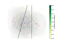
To illustrate our theoretical findings, we start by testing our learning algorithm on the following synthetic two-dimensional problem. Let us consider the distribution \mathbb{P} defined as (Y=±1)=1/2\mathbb{P}\left(Y=\pm 1\right)=1/2, (XY=1)=𝒩(0,I2)\mathbb{P}\left(X\mid Y=-1\right)=\mathcal{N}(0,I_{2}) and (XY=1)=12[𝒩((3,0),I2)+𝒩((3,0),I2)]\mathbb{P}\left(X\mid Y=1\right)=\frac{1}{2}\left[\mathcal{N}((-3,0),I_{2})+\mathcal{N}((3,0),I_{2})\right]. We sample 10001000 training points from this distribution and randomly generate 1010 linear classifiers that achieves a standard training risk lower than 0.40.4. To simulate an adversary with budget ε\varepsilon in 2\ell_{2} norm, we proceed as follows. For every sample (x,y)(x,y)\sim\mathbb{P} we generate 10001000 points uniformly at random in the ball of radius ε\varepsilon and select the one maximizing the risk for the 0/10/1 loss. Figure 2 (left) illustrates the type of mixture we get after convergence of our algorithms. Note that in this toy problem, we are likely to find the optimal adversary with this sampling strategy if we sample enough attack points.

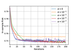
To evaluate the convergence of our algorithms, we compute the adversarial risk of our mixture for each iteration of both the oracle and regularized algorithms. Figure 2 illustrates the convergence of the algorithms w.r.t the regularization parameter. We observe that the risk for both algorithms converge. Moreover, they converge towards the oracle minimizer when the regularization parameter α\alpha goes to 0.

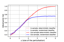
Finally, to demonstrate the improvement randomized techniques offer against deterministic defenses, we plot in Figure 2 (right) the minimum adversarial risk for both randomized and deterministic classifiers w.r.t. ε\varepsilon. The adversarial risk is strictly better for randomized classifier whenever the adversarial budget ε\varepsilon is bigger than 22. This illustration validates our analysis of Theorem 1, and motivates a in depth study of a more challenging framework, namely image classification with neural networks.

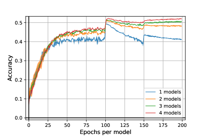
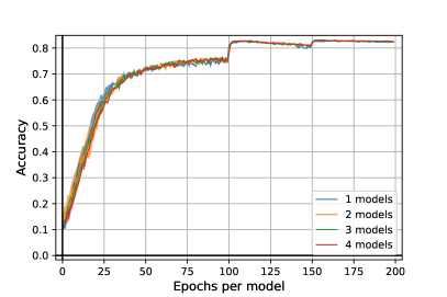
5.2 CIFAR-10 Dataset

Models Acc. APGDCE\textrm{APGD}_{\textrm{CE}} APGDDLR\textrm{APGD}_{\textrm{DLR}} Rob. Acc.
1 81.9%81.9\% 47.6%47.6\% 47.7%47.7\% 45.6%45.6\%
2 81.9%81.9\% 49.0%49.0\% 49.6%{49.6\%} 47.0%{47.0\%}
3 81.7%{81.7\%} 49.0%{49.0\%} 49.3%49.3\% 46.9%{46.9\%}
4 82.6%\bm{82.6\%} 49.7%\bm{49.7\%} 49.8%\bm{49.8}\% 47.2%\bm{47.2\%}
Refer to captionRefer to caption
Figure 3: On left: Comparison of our algorithm with a standard adversarial training (one model). We reported the results for the model with the best robust accuracy obtained over two independent runs because adversarial training might be unstable. Standard and Robust accuracy (respectively in the middle and on right) on CIFAR-10 test images in function of the number of epochs per classifier with 11 to 33 ResNet18 models. The performed attack is PGD with 2020 iterations and ε=8/255\varepsilon=8/255.

Adversarial examples are known to be easily transferrable from one model to another [35]. To counter this and support our theoretical claims, we propose an heuristic algorithm (see Algorithm 2) to train a robust mixture of LL classifiers. We alternatively train these classifiers with adversarial examples against the current mixture and update the probabilities of the mixture according to the algorithms we proposed in Section 4.2. More details on the heuristic algorithm are available in Appendix D.

LL: number of models, TT: number of iterations,
TθT_{\theta}: number of updates for the models 𝜽\bm{\theta},
TλT_{\lambda}: number of updates for the mixture 𝝀\bm{\lambda},
𝝀0=(λ01,λ0L),𝜽0=(θ01,θ0L)\bm{\lambda}_{0}=(\lambda_{0}^{1},\dots\lambda_{0}^{L}),~{}\bm{\theta}_{0}=(\theta_{0}^{1},\dots\theta_{0}^{L})
for t=1,,Tt=1,\dots,T do

       Let BtB_{t} be a batch of data.
if tmod(TθL+1)0t\mod(T_{\theta}L+1)\neq 0 then
             kk sampled uniformly in {1,,L}\{1,\dots,L\}
B~t\tilde{B}_{t}\leftarrow Attack of images in BtB_{t} for the model (𝝀t,𝜽t)(\bm{\lambda}_{t},\bm{\theta}_{t})
θkt\theta^{t}_{k}\leftarrow Update θkt1\theta^{t-1}_{k} with B~t\tilde{B}_{t} for fixed 𝝀t\bm{\lambda}_{t} with a SGD step
      else
             𝝀t\bm{\lambda}_{t}\leftarrowUpdate 𝝀t1\bm{\lambda}_{t-1} on BtB_{t} for fixed 𝜽t\bm{\theta}_{t} with oracle or regularized algorithm with TλT_{\lambda} iterations.
       end if
      
end for
Algorithm 2 Adversarial Training for Mixtures

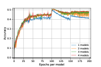
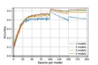
Experimental Setup. To evaluate the performance of Algorithm 2, we trained from 11 to 44 ResNet18 [20] models on 200200 epochs per model777L×200L\times 200 epochs in total, where LL is the number of models.. We study the robustness with regards to \ell_{\infty} norm and fixed adversarial budget ε=8/255\varepsilon=8/255. The attack we used in the inner maximization of the training is an adapted (adaptative) version of PGD for mixtures of classifiers with 1010 steps. Note that for one single model, Algorithm 2 exactly corresponds to adversarial training [24]. For each of our setups, we made two independent runs and select the best one. The training time of our algorithm is around four times longer than a standard Adversarial Training (with PGD 10 iter.) with two models, eight times with three models and twelve times with four models. We trained our models with a batch of size 10241024 on 88 Nvidia V100 GPUs. We give more details on implementation in Appendix D.

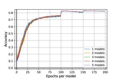
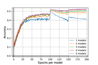
Evaluation Protocol. At each epoch, we evaluate the current mixture on test data against PGD attack with 2020 iterations. To select our model and avoid overfitting [30], we kept the most robust against this PGD attack. To make a final evaluation of our mixture of models, we used an adapted version of AutoPGD untargeted attacks [15] for randomized classifiers with both Cross-Entropy (CE) and Difference of Logits Ratio (DLR) loss. For both attacks, we made 100100 iterations and 55 restarts.

Results. The results are presented in Figure 3. We remark our algorithm outperforms a standard adversarial training in all the cases by more 1%1\%, without additional loss of standard accuracy as it is attested by the left figure. Moreover, it seems our algorithm, by adding more and more models, reduces the overfitting of adversarial training. So far, experiments are computationally very costful and it is difficult to raise precise conclusions. Further, hyperparameter tuning  [19] such as architecture, unlabeled data [12], activation function, or the use of TRADES [43] may still increase the results.

6 Related Work and Discussions

Distributionally Robust Optimization. Several recent works [33, 23, 37] studied the problem of adversarial examples through the scope of distributionally robust optimization. In these frameworks, the set of adversarial distributions is defined using an p\ell_{p} Wasserstein ball (the adversary is allowed to have an average perturbation of at most ε\varepsilon in p\ell_{p} norm). This however does not match the usual adversarial attack problem, where the adversary cannot move any point by more than ε\varepsilon. In the present work, we introduce a cost function allowing us to cast the adversarial example problem as a DRO one, without changing the adversary constraints.

Optimal Transport (OT). [5] and  [29] investigated classifier-agnostic lower bounds on the adversarial risk of any deterministic classifier using OT. These works only evaluate lower bounds on the primal deterministic formulation of the problem, while we study the existence of mixed Nash equilibria. Note that [29] started to investigate a way to formalize the adversary using Markov kernels, but did not investigate the impact of randomized strategies on the game. We extended this work by rigorously reformulating the adversarial risk as a linear optimization problem over distributions and we study this problem from a game theoretic point of view.

Game Theory. Adversarial examples have been studied under the notions of Stackelberg game in [10], and zero-sum game in [31, 26, 8]. These works considered restricted settings (convex loss, parametric adversaries, etc.) that do not comply with the nature of the problem. Indeed, we prove in Appendix C.3 that when the loss is convex and the set Θ\Theta is convex, the duality gap is zero for deterministic classifiers. However, it has been proven that no convex loss can be a good surrogate for the 0/10/1 loss in the adversarial setting [1, 14], narrowing the scope of this result. If one can show that for sufficiently separated conditional distributions, an optimal deterministic classifier always exists (see Appendix E for a clear statement), necessary and sufficient conditions for the need of randomization are still to be established.  [27] studied partly this question for regularized deterministic adversaries, leaving the general setting of randomized adversaries and mixed equilibria unanswered, which is the very scope of this paper.

References

  • [1] H. Bao, C. Scott, and M. Sugiyama. Calibrated surrogate losses for adversarially robust classification. In J. Abernethy and S. Agarwal, editors, Proceedings of Thirty Third Conference on Learning Theory, volume 125 of Proceedings of Machine Learning Research, pages 408–451. PMLR, 09–12 Jul 2020.
  • [2] P. L. Bartlett and S. Mendelson. Rademacher and gaussian complexities: Risk bounds and structural results. Journal of Machine Learning Research, 3:463–482, 2002.
  • [3] A. Beck and M. Teboulle. A fast iterative shrinkage-thresholding algorithm for linear inverse problems. SIAM journal on imaging sciences, 2(1):183–202, 2009.
  • [4] D. P. Bertsekas and S. Shreve. Stochastic optimal control: the discrete-time case. 2004.
  • [5] A. N. Bhagoji, D. Cullina, and P. Mittal. Lower bounds on adversarial robustness from optimal transport. In Advances in Neural Information Processing Systems 32, pages 7496–7508. Curran Associates, Inc., 2019.
  • [6] B. Biggio, I. Corona, D. Maiorca, B. Nelson, N. Šrndić, P. Laskov, G. Giacinto, and F. Roli. Evasion attacks against machine learning at test time. In Joint European conference on machine learning and knowledge discovery in databases, pages 387–402. Springer, 2013.
  • [7] J. Blanchet and K. Murthy. Quantifying distributional model risk via optimal transport. Mathematics of Operations Research, 44(2):565–600, 2019.
  • [8] A. J. Bose, G. Gidel, H. Berard, A. Cianflone, P. Vincent, S. Lacoste-Julien, and W. L. Hamilton. Adversarial example games, 2021.
  • [9] S. Boyd. Subgradient methods. 2003.
  • [10] M. Brückner and T. Scheffer. Stackelberg games for adversarial prediction problems. In Proceedings of the 17th ACM SIGKDD International Conference on Knowledge Discovery and Data Mining, KDD ’11, page 547–555, New York, NY, USA, 2011. Association for Computing Machinery.
  • [11] N. Carlini and D. Wagner. Adversarial examples are not easily detected: Bypassing ten detection methods. In Proceedings of the 10th ACM Workshop on Artificial Intelligence and Security, pages 3–14, 2017.
  • [12] Y. Carmon, A. Raghunathan, L. Schmidt, P. Liang, and J. C. Duchi. Unlabeled data improves adversarial robustness. arXiv preprint arXiv:1905.13736, 2019.
  • [13] J. M. Cohen, E. Rosenfeld, and J. Z. Kolter. Certified adversarial robustness via randomized smoothing. arXiv preprint arXiv:1902.02918.
  • [14] Z. Cranko, A. Menon, R. Nock, C. S. Ong, Z. Shi, and C. Walder. Monge blunts bayes: Hardness results for adversarial training. In K. Chaudhuri and R. Salakhutdinov, editors, Proceedings of the 36th International Conference on Machine Learning, volume 97 of Proceedings of Machine Learning Research, pages 1406–1415. PMLR, 09–15 Jun 2019.
  • [15] F. Croce and M. Hein. Reliable evaluation of adversarial robustness with an ensemble of diverse parameter-free attacks. In International Conference on Machine Learning, 2020.
  • [16] M. Cuturi. Sinkhorn distances: Lightspeed computation of optimal transport. Advances in neural information processing systems, 26:2292–2300, 2013.
  • [17] G. S. Dhillon, K. Azizzadenesheli, J. D. Bernstein, J. Kossaifi, A. Khanna, Z. C. Lipton, and A. Anandkumar. Stochastic activation pruning for robust adversarial defense. In International Conference on Learning Representations, 2018.
  • [18] I. Goodfellow, J. Shlens, and C. Szegedy. Explaining and harnessing adversarial examples. In International Conference on Learning Representations, 2015.
  • [19] S. Gowal, C. Qin, J. Uesato, T. Mann, and P. Kohli. Uncovering the limits of adversarial training against norm-bounded adversarial examples. arXiv preprint arXiv:2010.03593, 2020.
  • [20] K. He, X. Zhang, S. Ren, and J. Sun. Deep residual learning for image recognition. In The IEEE Conference on Computer Vision and Pattern Recognition (CVPR), 2016.
  • [21] A. Krizhevsky and G. Hinton. Learning multiple layers of features from tiny images. Technical report, Citeseer, 2009.
  • [22] A. Kurakin, I. Goodfellow, and S. Bengio. Adversarial examples in the physical world. arXiv preprint arXiv:1607.02533, 2016.
  • [23] J. Lee and M. Raginsky. Minimax statistical learning with wasserstein distances. In Advances in Neural Information Processing Systems 31, pages 2687–2696. Curran Associates, Inc., 2018.
  • [24] A. Madry, A. Makelov, L. Schmidt, D. Tsipras, and A. Vladu. Towards deep learning models resistant to adversarial attacks. In International Conference on Learning Representations, 2018.
  • [25] S.-M. Moosavi-Dezfooli, A. Fawzi, J. Uesato, and P. Frossard. Robustness via curvature regularization, and vice versa. In Proceedings of the IEEE Conference on Computer Vision and Pattern Recognition, pages 9078–9086, 2019.
  • [26] J. C. Perdomo and Y. Singer. Robust attacks against multiple classifiers. arXiv preprint arXiv:1906.02816, 2019.
  • [27] R. Pinot, R. Ettedgui, G. Rizk, Y. Chevaleyre, and J. Atif. Randomization matters. how to defend against strong adversarial attacks. International Conference on Machine Learning, 2020.
  • [28] R. Pinot, L. Meunier, A. Araujo, H. Kashima, F. Yger, C. Gouy-Pailler, and J. Atif. Theoretical evidence for adversarial robustness through randomization. In Advances in Neural Information Processing Systems, pages 11838–11848, 2019.
  • [29] M. S. Pydi and V. Jog. Adversarial risk via optimal transport and optimal couplings. In International Conference on Machine Learning. 2020.
  • [30] L. Rice, E. Wong, and Z. Kolter. Overfitting in adversarially robust deep learning. In International Conference on Machine Learning, pages 8093–8104. PMLR, 2020.
  • [31] S. Rota Bulò, B. Biggio, I. Pillai, M. Pelillo, and F. Roli. Randomized prediction games for adversarial machine learning. IEEE Transactions on Neural Networks and Learning Systems, 28(11):2466–2478, 2017.
  • [32] S. Shalev-Shwartz and S. Ben-David. Understanding machine learning: From theory to algorithms. Cambridge university press, 2014.
  • [33] A. Sinha, H. Namkoong, and J. Duchi. Certifying some distributional robustness with principled adversarial training. arXiv preprint arXiv:1710.10571, 2017.
  • [34] C. Szegedy, W. Zaremba, I. Sutskever, J. Bruna, D. Erhan, I. Goodfellow, and R. Fergus. Intriguing properties of neural networks. In International Conference on Learning Representations, 2014.
  • [35] F. Tramèr, N. Papernot, I. Goodfellow, D. Boneh, and P. McDaniel. The space of transferable adversarial examples. arXiv preprint arXiv:1704.03453, 2017.
  • [36] P. Tseng. On accelerated proximal gradient methods for convex-concave optimization. submitted to SIAM Journal on Optimization, 1, 2008.
  • [37] Z. Tu, J. Zhang, and D. Tao. Theoretical analysis of adversarial learning: A minimax approach. arXiv preprint arXiv:1811.05232, 2018.
  • [38] C. Villani. Topics in optimal transportation. Number 58. American Mathematical Soc., 2003.
  • [39] B. Wang, Z. Shi, and S. Osher. Resnets ensemble via the feynman-kac formalism to improve natural and robust accuracies. In Advances in Neural Information Processing Systems 32, pages 1655–1665. Curran Associates, Inc., 2019.
  • [40] C. Xie, J. Wang, Z. Zhang, Z. Ren, and A. Yuille. Mitigating adversarial effects through randomization. In International Conference on Learning Representations, 2018.
  • [41] M.-C. Yue, D. Kuhn, and W. Wiesemann. On linear optimization over wasserstein balls. arXiv preprint arXiv:2004.07162, 2020.
  • [42] S. Zagoruyko and N. Komodakis. Wide residual networks. In Proceedings of the British Machine Vision Conference (BMVC), pages 87.1–87.12. BMVA Press, 2016.
  • [43] H. Zhang, Y. Yu, J. Jiao, E. P. Xing, L. E. Ghaoui, and M. I. Jordan. Theoretically principled trade-off between robustness and accuracy. International conference on Machine Learning, 2019.

Supplementary material

Appendix A Notations

Let (𝒵,d)(\mathcal{Z},d) be a Polish metric space (i.e. complete and separable). We say that (𝒵,d)(\mathcal{Z},d) is proper if for all z0𝒵z_{0}\in\mathcal{Z} and R>0R>0, B(z0,R):={zd(z,z0)R}B(z_{0},R):=\{z\mid d(z,z_{0})\leq R\} is compact. For (𝒵,d)(\mathcal{Z},d) a Polish space, we denote +1(𝒵)\mathcal{M}_{+}^{1}(\mathcal{Z}) the set of Borel probability measures on 𝒵\mathcal{Z} endowed with TV\lVert\cdot\rVert_{TV} strong topology. We recall the notion of weak topology: we say that a sequence (μn)n(\mu_{n})_{n} of +1(𝒵)\mathcal{M}_{+}^{1}(\mathcal{Z}) converges weakly to μ+1(𝒵)\mu\in\mathcal{M}_{+}^{1}(\mathcal{Z}) if and only if for every continuous function ff on 𝒵\mathcal{Z}, f𝑑μnnf𝑑μ\int fd\mu_{n}\to_{n\to\infty}\int fd\mu. Endowed with its weak topology, +1(𝒵)\mathcal{M}_{+}^{1}(\mathcal{Z}) is a Polish space. For μ+1(𝒵)\mu\in\mathcal{M}_{+}^{1}(\mathcal{Z}), we define L1(μ)L^{1}(\mu) the set of integrable functions with respect to μ\mu. We denote Π1:(z,z)𝒵2z\Pi_{1}:(z,z^{\prime})\in\mathcal{Z}^{2}\mapsto z and Π2:(z,z)𝒵2z\Pi_{2}:(z,z^{\prime})\in\mathcal{Z}^{2}\mapsto z^{\prime} respectively the projections on the first and second component, which are continuous applications. For a measure μ\mu and a measurable mapping μ\mu, we denote gμg_{\sharp}\mu the pushforward measure of μ\mu by gg. Let L1L\geq 1 be an integer and denote ΔL:={λ+Ls.t.k=1Lλk=1}\Delta_{L}:=\{\lambda\in\mathbb{R}_{+}^{L}~{}\mathrm{s.t.}~{}\sum_{k=1}^{L}\lambda_{k}=1\}, the probability simplex of L\mathbb{R}^{L}.

Appendix B Useful Lemmas

Lemma 1 (Fubini’s theorem).

Let l:Θ×(𝒳×𝒴)[0,)l:\Theta\times(\mathcal{X}\times\mathcal{Y})\rightarrow[0,\infty) satisfying Assumption 1. Then for all μ+1(Θ)\mu\in\mathcal{M}^{1}_{+}(\Theta), l(θ,)𝑑μ(θ)\int l(\theta,\cdot)d\mu(\theta) is Borel measurable; for +1(𝒳×𝒴)\mathbb{Q}\in\mathcal{M}^{1}_{+}(\mathcal{X}\times\mathcal{Y}), l(,(x,y))𝑑(x,y)\int l(\cdot,(x,y))d\mathbb{Q}(x,y) is Borel measurable. Moreover: l(θ,(x,y))𝑑μ(θ)𝑑(x,y)=l(θ,(x,y))𝑑(x,y)𝑑μ(θ)\int l(\theta,(x,y))d\mu(\theta)d\mathbb{Q}(x,y)=\int l(\theta,(x,y))d\mathbb{Q}(x,y)d\mu(\theta)

Lemma 2.

Let l:Θ×(𝒳×𝒴)[0,)l:\Theta\times(\mathcal{X}\times\mathcal{Y})\rightarrow[0,\infty) satisfying Assumption 1. Then for all μ+1(Θ)\mu\in\mathcal{M}^{1}_{+}(\Theta), (x,y)l(θ,(x,y))𝑑μ(θ)(x,y)\mapsto\int l(\theta,(x,y))d\mu(\theta) is upper semi-continuous and hence Borel measurable.

Proof.

Let (xn,yn)n(x_{n},y_{n})_{n} be a sequence of 𝒳×𝒴\mathcal{X}\times\mathcal{Y} converging to (x,y)𝒳×𝒴(x,y)\in\mathcal{X}\times\mathcal{Y}. For all θΘ\theta\in\Theta, Ml(θ,)M-l(\theta,\cdot) is non negative and lower semi-continuous. Then by Fatou’s Lemma applied:

Ml(θ,(x,y))dμ(θ)\displaystyle\int M-l(\theta,(x,y))d\mu(\theta) lim infnMl(θ,(xn,yn))dμ(θ)\displaystyle\leq\int\liminf_{n\to\infty}M-l(\theta,(x_{n},y_{n}))d\mu(\theta)
lim infnMl(θ,(xn,yn))dμ(θ)\displaystyle\leq\liminf_{n\to\infty}\int M-l(\theta,(x_{n},y_{n}))d\mu(\theta)

Then we deduce that: Ml(θ,)dμ(θ)\int M-l(\theta,\cdot)d\mu(\theta) is lower semi-continuous and then l(θ,)𝑑μ(θ)\int l(\theta,\cdot)d\mu(\theta) is upper-semi continuous. ∎

Lemma 3.

Let l:Θ×(𝒳×𝒴)[0,)l:\Theta\times(\mathcal{X}\times\mathcal{Y})\rightarrow[0,\infty) satisfying Assumption 1 Then for all μ+1(Θ)\mu\in\mathcal{M}^{1}_{+}(\Theta), l(θ,(x,y))𝑑μ(θ)𝑑(x,y)\mathbb{Q}\mapsto\int l(\theta,(x,y))d\mu(\theta)d\mathbb{Q}(x,y) is upper semi-continuous for weak topology of measures.

Proof.

l(θ,)𝑑μ(θ)-\int l(\theta,\cdot)d\mu(\theta) is lower semi-continuous from Lemma 2. Then Ml(θ,)𝑑μ(θ)M-\int l(\theta,\cdot)d\mu(\theta) is lower semi-continuous and non negative. Let denote vv this function. Let (vn)n(v_{n})_{n} be a non-decreasing sequence of continuous bounded functions such that vnvv_{n}\to v. Let (k)k(\mathbb{Q}_{k})_{k} converging weakly towards \mathbb{Q}. Then by monotone convergence:

v𝑑=limnvn𝑑=limnlimkvn𝑑klim infkv𝑑k\displaystyle\int vd\mathbb{Q}=\lim_{n}\int v_{n}d\mathbb{Q}=\lim_{n}\lim_{k}\int v_{n}d\mathbb{Q}_{k}\leq\liminf_{k}\int vd\mathbb{Q}_{k}

Then v𝑑\mathbb{Q}\mapsto\int vd\mathbb{Q} is lower semi-continuous and then l(θ,(x,y))𝑑μ(θ)𝑑(x,y)\mathbb{Q}\mapsto\int l(\theta,(x,y))d\mu(\theta)d\mathbb{Q}(x,y) is upper semi-continuous for weak topology of measures. ∎

Lemma 4.

Let l:Θ×(𝒳×𝒴)[0,)l:\Theta\times(\mathcal{X}\times\mathcal{Y})\rightarrow[0,\infty) satisfying Assumption 1. Then for all μ+1(Θ)\mu\in\mathcal{M}^{1}_{+}(\Theta), (x,y)sup(x,y),d(x,x)ε,y=yl(θ,(x,y))𝑑μ(θ)(x,y)\mapsto\sup_{(x^{\prime},y^{\prime}),d(x,x^{\prime})\leq\varepsilon,y=y^{\prime}}\int l(\theta,(x^{\prime},y^{\prime}))d\mu(\theta) is universally measurable (i.e. measurable for all Borel probability measures). And hence the adversarial risk is well defined.

Proof.

Let ϕ:(x,y)sup(x,y),d(x,x)ε,y=yl(θ,(x,y))𝑑μ(θ)\phi:(x,y)\mapsto\sup_{(x^{\prime},y^{\prime}),d(x,x^{\prime})\leq\varepsilon,y=y^{\prime}}\int l(\theta,(x^{\prime},y^{\prime}))d\mu(\theta). Then for u¯u\in\bar{\mathbb{R}}:

{ϕ(x,y)>u}=Proj1{((x,y),(x,y))l(θ,(x,y))𝑑μ(θ)cε((x,y),(x,y))>u}\displaystyle\left\{\phi(x,y)>u\right\}=\text{Proj}_{1}\left\{((x,y),(x^{\prime},y^{\prime}))\mid\int l(\theta,(x^{\prime},y^{\prime}))d\mu(\theta)-c_{\varepsilon}((x,y),(x^{\prime},y^{\prime}))>u\right\}

By Lemma 3: ((x,y),(x,y))l(θ,(x,y))𝑑μ(θ)cε((x,y),(x,y))((x,y),(x^{\prime},y^{\prime}))\mapsto\int l(\theta,(x^{\prime},y^{\prime}))d\mu(\theta)-c_{\varepsilon}((x,y),(x^{\prime},y^{\prime})) is upper-semicontinuous hence Borel measurable. So its level sets are Borel sets, and by [4, Proposition 7.39], the projection of a Borel set is analytic. And then {ϕ(x,y)>u}\left\{\phi(x,y)>u\right\} universally measurable thanks to [4, Corollary 7.42.1]. We deduce that ϕ\phi is universally measurable. ∎

Appendix C Proofs

C.1 Proof of Proposition 1

Proof.

Let η>0\eta>0. Let 𝒜ε()\mathbb{Q}\in\mathcal{A}_{\varepsilon}(\mathbb{P}). There exists γ1+((𝒳×𝒴)2)\gamma\in\mathcal{M}^{+}_{1}\left((\mathcal{X}\times\mathcal{Y})^{2}\right) such that, d(x,x)εd(x,x^{\prime})\leq\varepsilon, y=yy=y^{\prime} γ\gamma-almost surely, and Π1γ=\Pi_{1\sharp}\gamma=\mathbb{P}, and Π2γ=\Pi_{2\sharp}\gamma=\mathbb{Q}. Then cε𝑑γ=0η\int c_{\varepsilon}d\gamma=0\leq\eta. Then, we deduce that Wcε(,)ηW_{c_{\varepsilon}}(\mathbb{P},\mathbb{Q})\leq\eta, and cε(,η)\mathbb{Q}\in\mathcal{B}_{c_{\varepsilon}}(\mathbb{P},\eta). Reciprocally, let cε(,η)\mathbb{Q}\in\mathcal{B}_{c_{\varepsilon}}(\mathbb{P},\eta). Then, since the infimum is attained in the Wasserstein definition, there exists γ1+((𝒳×𝒴)2)\gamma\in\mathcal{M}^{+}_{1}\left((\mathcal{X}\times\mathcal{Y})^{2}\right) such that cε𝑑γη\int c_{\varepsilon}d\gamma\leq\eta. Since cε((x,x),(y,y))=+c_{\varepsilon}((x,x^{\prime}),(y,y^{\prime}))=+\infty when d(x,x)>εd(x,x^{\prime})>\varepsilon and yyy\neq y^{\prime}, we deduce that, d(x,x)εd(x,x^{\prime})\leq\varepsilon and y=yy=y^{\prime}, γ\gamma-almost surely. Then 𝒜ε()\mathbb{Q}\in\mathcal{A}_{\varepsilon}(\mathbb{P}). We have then shown that: 𝒜ε()=cε(,η)\mathcal{A}_{\varepsilon}(\mathbb{P})=\mathcal{B}_{c_{\varepsilon}}(\mathbb{P},\eta).

The convexity of 𝒜ε()\mathcal{A}_{\varepsilon}(\mathbb{P}) is then immediate from the relation with the Wasserstein uncertainty set.

Let us show first that 𝒜ε()\mathcal{A}_{\varepsilon}(\mathbb{P}) is relatively compact for weak topology. To do so we will show that 𝒜ε()\mathcal{A}_{\varepsilon}(\mathbb{P}) is tight and apply Prokhorov’s theorem. Let δ>0\delta>0, (𝒳×𝒴,dd)(\mathcal{X}\times\mathcal{Y},d\oplus d^{\prime}) being a Polish space, {}\{\mathbb{P}\} is tight then there exists KδK_{\delta} compact such that (Kδ)1δ\mathbb{P}(K_{\delta})\geq 1-\delta. Let K~δ:={(x,y)(x,y)Kδ,d(x,x)ε,y=y}\tilde{K}_{\delta}:=\left\{(x^{\prime},y^{\prime})\mid\exists(x,y)\in K_{\delta},~{}d(x^{\prime},x)\leq\varepsilon,~{}y=y^{\prime}\right\}. Recalling that (𝒳,d)(\mathcal{X},d) is proper (i.e. the closed balls are compact), so K~δ\tilde{K}_{\delta} is compact. Moreover for 𝒜ε()\mathbb{Q}\in\mathcal{A}_{\varepsilon}(\mathbb{P}), (K~δ)(Kδ)1δ\mathbb{Q}(\tilde{K}_{\delta})\geq\mathbb{P}(K_{\delta})\geq 1-\delta. And then, Prokhorov’s theorem holds, and 𝒜ε()\mathcal{A}_{\varepsilon}(\mathbb{P}) is relatively compact for weak topology.

Let us now prove that 𝒜ε()\mathcal{A}_{\varepsilon}(\mathbb{P}) is closed to conclude. Let (n)n(\mathbb{Q}_{n})_{n} be a sequence of 𝒜ε()\mathcal{A}_{\varepsilon}(\mathbb{P}) converging towards some \mathbb{Q} for weak topology. For each nn, there exists γn+1(𝒳×𝒴)\gamma_{n}\in\mathcal{M}^{1}_{+}(\mathcal{X}\times\mathcal{Y}) such that d(x,x)εd(x,x^{\prime})\leq\varepsilon and y=yy=y^{\prime} γn\gamma_{n}-almost surely and Π1γn=\Pi_{1\sharp}\gamma_{n}=\mathbb{P}, Π2γn=n\Pi_{2\sharp}\gamma_{n}=\mathbb{Q}_{n}. {n,n0}\{\mathbb{Q}_{n},n\geq 0\} is relatively compact, then tight, then nΓ,n\bigcup_{n}\Gamma_{\mathbb{P},\mathbb{Q}_{n}} is tight, then relatively compact by Prokhorov’s theorem. (γn)nnΓ,n(\gamma_{n})_{n}\in\bigcup_{n}\Gamma_{\mathbb{P},\mathbb{Q}_{n}}, then up to an extraction, γnγ\gamma_{n}\to\gamma. Then d(x,x)εd(x,x^{\prime})\leq\varepsilon and y=yy=y^{\prime} γ\gamma-almost surely, and by continuity, Π1γ=\Pi_{1\sharp}\gamma=\mathbb{P} and by continuity, Π2γ=\Pi_{2\sharp}\gamma=\mathbb{Q}. And hence 𝒜ε()\mathcal{A}_{\varepsilon}(\mathbb{P}) is closed.

Finally 𝒜ε()\mathcal{A}_{\varepsilon}(\mathbb{P}) is a convex compact set for the weak topology. ∎

C.2 Proof of Proposition 2

Proof.

Let μ+1(Θ)\mu\in\mathcal{M}^{1}_{+}(\Theta). Let f~:((x,y),(x,y))𝔼θμ[l(θ,(x,y))]cε((x,y),(x,y))\tilde{f}:((x,y),(x^{\prime},y^{\prime}))\mapsto\mathbb{E}_{\theta\sim\mu}\left[l(\theta,(x,y))\right]-c_{\varepsilon}((x,y),(x^{\prime},y^{\prime})). f~\tilde{f} is upper-semi continuous, hence upper semi-analytic. Then, by upper semi continuity of 𝔼θμ[l(θ,)]\mathbb{E}_{\theta\sim\mu}\left[l(\theta,\cdot)\right] on the compact {(x,y)d(x,x)ε,y=y}\{(x^{\prime},y^{\prime})\mid~{}d(x,x^{\prime})\leq\varepsilon,y=y^{\prime}\} and [4, Proposition 7.50], there exists a universally measurable mapping TT such that 𝔼θμ[l(θ,T(x,y))]=sup(x,y),d(x,x)ε,y=y𝔼θμ[l(θ,(x,y))]\mathbb{E}_{\theta\sim\mu}\left[l(\theta,T(x,y))\right]=\sup_{(x^{\prime},y^{\prime}),~{}d(x,x^{\prime})\leq\varepsilon,y=y^{\prime}}\mathbb{E}_{\theta\sim\mu}\left[l(\theta,(x,y))\right]. Let =T\mathbb{Q}=T_{\sharp}\mathbb{P}, then 𝒜ε()\mathbb{Q}\in\mathcal{A}_{\varepsilon}(\mathbb{P}). And then 𝔼(x,y)[sup(x,y),d(x,x)ε,y=y𝔼θμ[l(θ,(x,y))]]sup𝒜ε()𝔼(x,y)[𝔼θμ[l(θ,(x,y))]]\mathbb{E}_{(x,y)\sim\mathbb{P}}\left[\sup_{(x^{\prime},y^{\prime}),~{}d(x,x^{\prime})\leq\varepsilon,y=y^{\prime}}\mathbb{E}_{\theta\sim\mu}\left[l(\theta,(x^{\prime},y^{\prime}))\right]\right]\leq\sup_{\mathbb{Q}\in\mathcal{A}_{\varepsilon}(\mathbb{P})}\mathbb{E}_{(x,y)\sim\mathbb{Q}}\left[\mathbb{E}_{\theta\sim\mu}\left[l(\theta,(x,y))\right]\right].

Reciprocally, let 𝒜ε()\mathbb{Q}\in\mathcal{A}_{\varepsilon}(\mathbb{P}). There exists γ+1((𝒳×𝒴)2)\gamma\in\mathcal{M}^{1}_{+}((\mathcal{X}\times\mathcal{Y})^{2}), such that d(x,x)εd(x,x^{\prime})\leq\varepsilon and y=yy=y^{\prime} γ\gamma-almost surely, and, Π1γ=\Pi_{1\sharp}\gamma=\mathbb{P} and Π2γ=\Pi_{2\sharp}\gamma=\mathbb{Q}. Then: 𝔼θμ[l(θ,(x,y))]sup(u,v),d(x,u)ε,y=v𝔼θμ[l(θ,(u,v))]\mathbb{E}_{\theta\sim\mu}\left[l(\theta,(x^{\prime},y^{\prime}))\right]\leq\sup_{(u,v),~{}d(x,u)\leq\varepsilon,y=v}\mathbb{E}_{\theta\sim\mu}\left[l(\theta,(u,v))\right] γ\gamma-almost surely. Then, we deduce that:

𝔼(x,y)[𝔼θμ[l(θ,(x,y))]]\displaystyle\mathbb{E}_{(x^{\prime},y^{\prime})\sim\mathbb{Q}}\left[\mathbb{E}_{\theta\sim\mu}\left[l(\theta,(x^{\prime},y^{\prime}))\right]\right] =𝔼(x,y,x,y)γ[𝔼θμ[l(θ,(x,y))]]\displaystyle=\mathbb{E}_{(x,y,x^{\prime},y^{\prime})\sim\gamma}\left[\mathbb{E}_{\theta\sim\mu}\left[l(\theta,(x^{\prime},y^{\prime}))\right]\right]
𝔼(x,y,x,y)γ[sup(u,v),d(x,u)ε,y=v𝔼θμ[l(θ,(u,v))]]\displaystyle\leq\mathbb{E}_{(x,y,x^{\prime},y^{\prime})\sim\gamma}\left[\sup_{(u,v),~{}d(x,u)\leq\varepsilon,y=v}\mathbb{E}_{\theta\sim\mu}\left[l(\theta,(u,v))\right]\right]
𝔼(x,y)[sup(u,v),d(x,u)ε,y=v𝔼θμ[l(θ,(u,v))]]\displaystyle\leq\mathbb{E}_{(x,y)\sim\mathbb{P}}\left[\sup_{(u,v),~{}d(x,u)\leq\varepsilon,y=v}\mathbb{E}_{\theta\sim\mu}\left[l(\theta,(u,v))\right]\right]

Then we deduce the expected result:

advε(μ)=sup𝒜ε()𝔼(x,y)[𝔼θμ[l(θ,(x,y))]]\displaystyle\mathcal{R}_{adv}^{\varepsilon}(\mu)=\sup_{\mathbb{Q}\in\mathcal{A}_{\varepsilon}(\mathbb{P})}\mathbb{E}_{(x,y)\sim\mathbb{Q}}\left[\mathbb{E}_{\theta\sim\mu}\left[l(\theta,(x,y))\right]\right]

Let us show that the optimum is attained. 𝔼(x,y)[𝔼θμ[l(θ,(x,y))]]\mathbb{Q}\mapsto\mathbb{E}_{(x,y)\sim\mathbb{Q}}\left[\mathbb{E}_{\theta\sim\mu}\left[l(\theta,(x,y))\right]\right] is upper semi continuous by Lemma 3 for the weak topology of measures, and 𝒜ε()\mathcal{A}_{\varepsilon}(\mathbb{P}) is compact by Proposition 1, then by [4, Proposition 7.32], the supremum is attained for a certain 𝒜ε()\mathbb{Q}^{*}\in\mathcal{A}_{\varepsilon}(\mathbb{P}).

C.3 Proof of Theorem 1

Let us first recall the Fan’s Theorem.

Theorem 2.

Let UU be a compact convex Haussdorff space and VV be convex space (not necessarily topological). Let ψ:U×V\psi:U\times V\to\mathbb{R} be a concave-convex function such that for all vVv\in V, ψ(,v)\psi(\cdot,v) is upper semi-continuous then:

infvVmaxuUψ(u,v)=maxuUinfvVψ(u,v)\displaystyle\inf_{v\in V}\max_{u\in U}\psi(u,v)=\max_{u\in U}\inf_{v\in V}\psi(u,v)

We are now set to prove Theorem 1.

Proof.

𝒜ε()\mathcal{A}_{\varepsilon}(\mathbb{P}), endowed with the weak topology of measures, is a Hausdorff compact convex space, thanks to Proposition 1. Moreover, +1(Θ)\mathcal{M}^{1}_{+}(\Theta) is clearly convex and (,μ)l𝑑μ𝑑(\mathbb{Q},\mu)\mapsto\int ld\mu d\mathbb{Q} is bilinear, hence concave-convex. Moreover thanks to Lemma 3, for all μ\mu, l𝑑μ𝑑\mathbb{Q}\mapsto\int ld\mu d\mathbb{Q} is upper semi-continuous. Then Fan’s theorem applies and strong duality holds. ∎

In the related work (Section 6), we mentioned a particular form of Theorem 1 for convex cases. As mentioned, this result has limited impact in the adversarial classification setting. It is still a direct corollary of Fan’s theorem. This theorem can be stated as follows:

Theorem 3.

Let +1(𝒳×𝒴)\mathbb{P}\in\mathcal{M}^{1}_{+}(\mathcal{X}\times\mathcal{Y}), ε>0\varepsilon>0 and Θ\Theta a convex set. Let ll be a loss satisfying Assumption 1, and also, (x,y)𝒳×𝒴(x,y)\in\mathcal{X}\times\mathcal{Y}, l(,(x,y))l(\cdot,(x,y)) is a convex function, then we have the following:

infθΘsup𝒜ε()𝔼[l(θ,(x,y))]=sup𝒜ε()infθΘ𝔼[l(θ,(x,y))]\displaystyle\inf_{\theta\in\Theta}\sup_{\mathbb{Q}\in\mathcal{A}_{\varepsilon}(\mathbb{P})}\mathbb{E}_{\mathbb{Q}}\left[l(\theta,(x,y))\right]=\sup_{\mathbb{Q}\in\mathcal{A}_{\varepsilon}(\mathbb{P})}\inf_{\theta\in\Theta}\mathbb{E}_{\mathbb{Q}}\left[l(\theta,(x,y))\right]

The supremum is always attained. If Θ\Theta is a compact set then, the infimum is also attained.

C.4 Proof of Proposition 3

Proof.

Let us first show that for α0\alpha\geq 0, supiΓi,ε𝔼i,μ[l(θ,(x,y))]αKL(i||1N𝕌(xi,yi))\sup_{\mathbb{Q}_{i}\in\Gamma_{i,\varepsilon}}\mathbb{E}_{\mathbb{Q}_{i},\mu}\left[l(\theta,(x,y))\right]-\alpha\text{KL}\left(\mathbb{Q}_{i}\Big{|}\Big{|}\frac{1}{N}\mathbb{U}_{(x_{i},y_{i})}\right) admits a solution. Let α0\alpha\geq 0, (α,in)n0(\mathbb{Q}_{\alpha,i}^{n})_{n\geq 0} a sequence such that

𝔼α,in,μ[l(θ,(x,y))]αKL(α,in||1N𝕌(xi,yi))n+supiΓi,ε𝔼i,μ[l(θ,(x,y))]αKL(i||1N𝕌(xi,yi)).\displaystyle\mathbb{E}_{\mathbb{Q}_{\alpha,i}^{n},\mu}\left[l(\theta,(x,y))\right]-\alpha\text{KL}\left(\mathbb{Q}_{\alpha,i}^{n}\Big{|}\Big{|}\frac{1}{N}\mathbb{U}_{(x_{i},y_{i})}\right)\xrightarrow[n\to+\infty]{}\sup_{\mathbb{Q}_{i}\in\Gamma_{i,\varepsilon}}\mathbb{E}_{\mathbb{Q}_{i},\mu}\left[l(\theta,(x,y))\right]-\alpha\text{KL}\left(\mathbb{Q}_{i}\Big{|}\Big{|}\frac{1}{N}\mathbb{U}_{(x_{i},y_{i})}\right).

As Γi,ε\Gamma_{i,\varepsilon} is tight ((𝒳,d)(\mathcal{X},d) is a proper metric space therefore all the closed ball are compact) and by Prokhorov’s theorem, we can extract a subsequence which converges toward α,i\mathbb{Q}^{*}_{\alpha,i}. Moreover, ll is upper semi-continuous (u.s.c), thus 𝔼,μ[l(θ,(x,y))]\mathbb{Q}\rightarrow\mathbb{E}_{\mathbb{Q},\mu}\left[l(\theta,(x,y))\right] is also u.s.c.888Indeed by considering a decreasing sequence of continuous and bounded functions which converge towards 𝔼μ[l(θ,(x,y))]\mathbb{E}_{\mu}\left[l(\theta,(x,y))\right] and by definition of the weak convergence the result follows. Moreover αKL(||1N𝕌(xi,yi))\mathbb{Q}\rightarrow-\alpha\text{KL}\left(\mathbb{Q}\Big{|}\Big{|}\frac{1}{N}\mathbb{U}_{(x_{i},y_{i})}\right) is also u.s.c. 999for α=0\alpha=0 the result is clear, and if α>0\alpha>0, note that KL(||1N𝕌(xi,yi))\text{KL}\left(\cdot\Big{|}\Big{|}\frac{1}{N}\mathbb{U}_{(x_{i},y_{i})}\right) is lower semi-continuous, therefore, by considering the limit superior as nn goes to infinity we obtain that

lim supn+𝔼α,in,μ[l(θ,(x,y))]αKL(α,in||1N𝕌(xi,yi))\displaystyle\limsup_{n\to+\infty}\mathbb{E}_{\mathbb{Q}_{\alpha,i}^{n},\mu}\left[l(\theta,(x,y))\right]-\alpha\text{KL}\left(\mathbb{Q}_{\alpha,i}^{n}\Big{|}\Big{|}\frac{1}{N}\mathbb{U}_{(x_{i},y_{i})}\right)
=supiΓi,ε𝔼i,μ[l(θ,(x,y))]αKL(i||1N𝕌(xi,yi))\displaystyle=\sup_{\mathbb{Q}_{i}\in\Gamma_{i,\varepsilon}}\mathbb{E}_{\mathbb{Q}_{i},\mu}\left[l(\theta,(x,y))\right]-\alpha\text{KL}\left(\mathbb{Q}_{i}\Big{|}\Big{|}\frac{1}{N}\mathbb{U}_{(x_{i},y_{i})}\right)
𝔼α,i,μ[l(θ,(x,y))]αKL(α,i||1N𝕌(xi,yi))\displaystyle\leq\mathbb{E}_{\mathbb{Q}_{\alpha,i}^{*},\mu}\left[l(\theta,(x,y))\right]-\alpha\text{KL}\left(\mathbb{Q}_{\alpha,i}^{*}\Big{|}\Big{|}\frac{1}{N}\mathbb{U}_{(x_{i},y_{i})}\right)

from which we deduce that α,i\mathbb{Q}_{\alpha,i}^{*} is optimal.

Let us now show the result. We consider a positive sequence of (αi())0(\alpha_{i}^{(\ell)})_{\ell\geq 0} such that αi()0\alpha_{i}^{(\ell)}\to 0. Let us denote αi(),i\mathbb{Q}^{*}_{\alpha_{i}^{(\ell)},i} and i\mathbb{Q}^{*}_{i} the solutions of maxiΓi,ε𝔼i,μ[l(θ,(x,y))]αi()KL(i||1N𝕌(xi,yi))\max_{\mathbb{Q}_{i}\in\Gamma_{i,\varepsilon}}\mathbb{E}_{\mathbb{Q}_{i},\mu}\left[l(\theta,(x,y))\right]-\alpha_{i}^{(\ell)}\text{KL}\left(\mathbb{Q}_{i}\Big{|}\Big{|}\frac{1}{N}\mathbb{U}_{(x_{i},y_{i})}\right) and maxiΓi,ε𝔼i,μ[l(θ,(x,y))]\max_{\mathbb{Q}_{i}\in\Gamma_{i,\varepsilon}}\mathbb{E}_{\mathbb{Q}_{i},\mu}\left[l(\theta,(x,y))\right] respectively. Since Γi,ε\Gamma_{i,\varepsilon} is tight, (αi(),i)0(\mathbb{Q}^{*}_{\alpha_{i}^{(\ell)},i})_{\ell\geq 0} is also tight and we can extract by Prokhorov’s theorem a subsequence which converges towards \mathbb{Q}^{*}. Moreover we have

𝔼i,μ[l(θ,(x,y))]αi()KL(i||1N𝕌(xi,yi))𝔼αi(),i,μ[l(θ,(x,y))]αi()KL(αi(),i||1N𝕌(xi,yi))\displaystyle\mathbb{E}_{\mathbb{Q}^{*}_{i},\mu}\left[l(\theta,(x,y))\right]-\alpha_{i}^{(\ell)}\text{KL}\left(\mathbb{Q}^{*}_{i}\Big{|}\Big{|}\frac{1}{N}\mathbb{U}_{(x_{i},y_{i})}\right)\leq\mathbb{E}_{\mathbb{Q}^{*}_{\alpha_{i}^{(\ell)},i},\mu}\left[l(\theta,(x,y))\right]-\alpha_{i}^{(\ell)}\text{KL}\left(\mathbb{Q}^{*}_{\alpha_{i}^{(\ell)},i}\Big{|}\Big{|}\frac{1}{N}\mathbb{U}_{(x_{i},y_{i})}\right)

from which follows that

0𝔼i,μ[l(θ,(x,y))]𝔼αi(),i,μ[l(θ,(x,y))]αi()(KL(i||1N𝕌(xi,yi))KL(αi(),i||1N𝕌(xi,yi)))\displaystyle 0\leq\mathbb{E}_{\mathbb{Q}^{*}_{i},\mu}\left[l(\theta,(x,y))\right]-\mathbb{E}_{\mathbb{Q}^{*}_{\alpha_{i}^{(\ell)},i},\mu}\left[l(\theta,(x,y))\right]\leq\alpha_{i}^{(\ell)}\left(\text{KL}\left(\mathbb{Q}^{*}_{i}\Big{|}\Big{|}\frac{1}{N}\mathbb{U}_{(x_{i},y_{i})}\right)-\text{KL}\left(\mathbb{Q}^{*}_{\alpha_{i}^{(\ell)},i}\Big{|}\Big{|}\frac{1}{N}\mathbb{U}_{(x_{i},y_{i})}\right)\right)

Then by considering the limit superior we obtain that

lim sup+𝔼αi(),i,μ[l(θ,(x,y))]=𝔼i,μ[l(θ,(x,y))].\displaystyle\limsup_{\ell\to+\infty}\mathbb{E}_{\mathbb{Q}^{*}_{\alpha_{i}^{(\ell)},i},\mu}\left[l(\theta,(x,y))\right]=\mathbb{E}_{\mathbb{Q}^{*}_{i},\mu}\left[l(\theta,(x,y))\right].

from which follows that

𝔼i,μ[l(θ,(x,y))]𝔼,μ[l(θ,(x,y))]\displaystyle\mathbb{E}_{\mathbb{Q}^{*}_{i},\mu}\left[l(\theta,(x,y))\right]\leq\mathbb{E}_{\mathbb{Q}^{*},\mu}\left[l(\theta,(x,y))\right]

and by optimality of i\mathbb{Q}^{*}_{i} we obtain the desired result. ∎

C.5 Proof of Proposition 4

Proof.

Let us denote for all μ1+(Θ)\mu\in\mathcal{M}_{1}^{+}(\Theta),

^adv,𝜶𝜺,m(μ):=i=1NαiNlog(1mij=1miexp𝔼μ[l(θ,uj(i))]αi).\displaystyle\widehat{\mathcal{R}}^{\bm{\varepsilon},\textbf{m}}_{adv,\bm{\alpha}}(\mu):=\sum_{i=1}^{N}\frac{\alpha_{i}}{N}\log\left(\frac{1}{m_{i}}\sum_{j=1}^{m_{i}}\exp\frac{\mathbb{E}_{\mu}\left[l(\theta,u_{j}^{(i)})\right]}{\alpha_{i}}\right).

Let also consider (μn(m))n0(\mu^{(\textbf{m})}_{n})_{n\geq 0} and (μn)n0(\mu_{n})_{n\geq 0} two sequences such that

^adv,𝜶𝜺,m(μn(m))n+^adv,𝜶𝜺,m,^adv,𝜶𝜺(μn)n+^adv,𝜶𝜺,.\displaystyle\widehat{\mathcal{R}}^{\bm{\varepsilon},\textbf{m}}_{adv,\bm{\alpha}}(\mu^{(\textbf{m})}_{n})\xrightarrow[n\to+\infty]{}\widehat{\mathcal{R}}^{\bm{\varepsilon},\textbf{m}}_{adv,\bm{\alpha}},~{}\quad\widehat{\mathcal{R}}^{\bm{\varepsilon}}_{adv,\bm{\alpha}}(\mu_{n})\xrightarrow[n\to+\infty]{}\widehat{\mathcal{R}}^{\bm{\varepsilon},*}_{adv,\bm{\alpha}}.

We first remarks that

^adv,𝜶𝜺,m^adv,𝜶𝜺,\displaystyle\widehat{\mathcal{R}}^{\bm{\varepsilon},\textbf{m}}_{adv,\bm{\alpha}}-\widehat{\mathcal{R}}^{\bm{\varepsilon},*}_{adv,\bm{\alpha}} ^adv,𝜶𝜺,m^adv,𝜶𝜺,m(μn)+^adv,𝜶𝜺,m(μn)^adv,𝜶𝜺(μn)+^adv,𝜶𝜺(μn)^adv,𝜶𝜺,\displaystyle\leq\widehat{\mathcal{R}}^{\bm{\varepsilon},\textbf{m}}_{adv,\bm{\alpha}}-\widehat{\mathcal{R}}^{\bm{\varepsilon},\textbf{m}}_{adv,\bm{\alpha}}(\mu_{n})+\widehat{\mathcal{R}}^{\bm{\varepsilon},\textbf{m}}_{adv,\bm{\alpha}}(\mu_{n})-\widehat{\mathcal{R}}^{\bm{\varepsilon}}_{adv,\bm{\alpha}}(\mu_{n})+\widehat{\mathcal{R}}^{\bm{\varepsilon}}_{adv,\bm{\alpha}}(\mu_{n})-\widehat{\mathcal{R}}^{\bm{\varepsilon},*}_{adv,\bm{\alpha}}
supμ1+(Θ)|^adv,𝜶𝜺,m(μ)^adv,𝜶𝜺(μ)|+^adv,𝜶𝜺(μn)^adv,𝜶𝜺,,\displaystyle\leq\sup_{\mu\in\mathcal{M}^{+}_{1}(\Theta)}\Big{|}\widehat{\mathcal{R}}^{\bm{\varepsilon},\textbf{m}}_{adv,\bm{\alpha}}(\mu)-\widehat{\mathcal{R}}^{\bm{\varepsilon}}_{adv,\bm{\alpha}}(\mu)\Big{|}+\widehat{\mathcal{R}}^{\bm{\varepsilon}}_{adv,\bm{\alpha}}(\mu_{n})-\widehat{\mathcal{R}}^{\bm{\varepsilon},*}_{adv,\bm{\alpha}},

and by considering the limit, we obtain that

^adv,𝜶𝜺,m^adv,𝜶𝜺,\displaystyle\widehat{\mathcal{R}}^{\bm{\varepsilon},\textbf{m}}_{adv,\bm{\alpha}}-\widehat{\mathcal{R}}^{\bm{\varepsilon},*}_{adv,\bm{\alpha}} supμ1+(Θ)|^adv,𝜶𝜺,m(μ)^adv,𝜶𝜺(μ)|\displaystyle\leq\sup_{\mu\in\mathcal{M}^{+}_{1}(\Theta)}\Big{|}\widehat{\mathcal{R}}^{\bm{\varepsilon},\textbf{m}}_{adv,\bm{\alpha}}(\mu)-\widehat{\mathcal{R}}^{\bm{\varepsilon}}_{adv,\bm{\alpha}}(\mu)\Big{|}

Simarly we have that

^adv,𝜶𝜺,^adv,𝜶𝜺,m\displaystyle\widehat{\mathcal{R}}^{\bm{\varepsilon},*}_{adv,\bm{\alpha}}-\widehat{\mathcal{R}}^{\bm{\varepsilon},\textbf{m}}_{adv,\bm{\alpha}} ^adv,𝜶𝜺,^adv,𝜶𝜺(μn(𝒎))+^adv,𝜶𝜺(μn(𝒎))^adv,𝜶𝜺,m(μn(𝒎))+^adv,𝜶𝜺,m(μn(𝒎))^adv,𝜶𝜺,m\displaystyle\leq\widehat{\mathcal{R}}^{\bm{\varepsilon},*}_{adv,\bm{\alpha}}-\widehat{\mathcal{R}}^{\bm{\varepsilon}}_{adv,\bm{\alpha}}(\mu_{n}^{(\bm{m})})+\widehat{\mathcal{R}}^{\bm{\varepsilon}}_{adv,\bm{\alpha}}(\mu_{n}^{(\bm{m})})-\widehat{\mathcal{R}}^{\bm{\varepsilon},\textbf{m}}_{adv,\bm{\alpha}}(\mu_{n}^{(\bm{m})})+\widehat{\mathcal{R}}^{\bm{\varepsilon},\textbf{m}}_{adv,\bm{\alpha}}(\mu_{n}^{(\bm{m})})-\widehat{\mathcal{R}}^{\bm{\varepsilon},\textbf{m}}_{adv,\bm{\alpha}}

from which follows that

^adv,𝜶𝜺,^adv,𝜶𝜺,m\displaystyle\widehat{\mathcal{R}}^{\bm{\varepsilon},*}_{adv,\bm{\alpha}}-\widehat{\mathcal{R}}^{\bm{\varepsilon},\textbf{m}}_{adv,\bm{\alpha}} supμ1+(Θ)|^adv,𝜶𝜺,m(μ)^adv,𝜶𝜺(μ)|\displaystyle\leq\sup_{\mu\in\mathcal{M}^{+}_{1}(\Theta)}\Big{|}\widehat{\mathcal{R}}^{\bm{\varepsilon},\textbf{m}}_{adv,\bm{\alpha}}(\mu)-\widehat{\mathcal{R}}^{\bm{\varepsilon}}_{adv,\bm{\alpha}}(\mu)\Big{|}

Therefore we obtain that

|^adv,𝜶𝜺,^adv,𝜶𝜺,m|i=1NαN\displaystyle\Big{|}\widehat{\mathcal{R}}^{\bm{\varepsilon},*}_{adv,\bm{\alpha}}-\widehat{\mathcal{R}}^{\bm{\varepsilon},\textbf{m}}_{adv,\bm{\alpha}}\Big{|}\leq\sum_{i=1}^{N}\frac{\alpha}{N} supμ1+(Θ)|log(1mij=1miexp(𝔼θμ[l(θ,uj(i)))]α))\displaystyle\sup_{\mu\in\mathcal{M}^{+}_{1}(\Theta)}\Big{|}\log\left(\frac{1}{m_{i}}\sum_{j=1}^{m_{i}}\exp\left(\frac{\mathbb{E}_{\theta\sim\mu}\left[l(\theta,u_{j}^{(i)}))\right]}{\alpha}\right)\right)
log(𝒳×𝒴exp(𝔼θμ[l(θ,(x,y))]α)d𝕌(xi,yi))|.\displaystyle-\log\left(\int_{\mathcal{X}\times\mathcal{Y}}\exp\left(\frac{\mathbb{E}_{\theta\sim\mu}\left[l(\theta,(x,y))\right]}{\alpha}\right)d\mathbb{U}_{(x_{i},y_{i})}\right)\Big{|}.

Observe that l0l\geq 0, therefore because the log\log function is 1-Lipschitz on [1,+)[1,+\infty), we obtain that

|^adv,𝜶𝜺,^adv,𝜶𝜺,m|i=1NαNsupμ1+(Θ)|1mij=1miexp(𝔼θμ[l(θ,uj(i)))]α)𝒳×𝒴exp(𝔼θμ[l(θ,(x,y))]α)𝑑𝕌(xi,yi)|.\displaystyle\Big{|}\widehat{\mathcal{R}}^{\bm{\varepsilon},*}_{adv,\bm{\alpha}}-\widehat{\mathcal{R}}^{\bm{\varepsilon},\textbf{m}}_{adv,\bm{\alpha}}\Big{|}\leq\sum_{i=1}^{N}\frac{\alpha}{N}\sup_{\mu\in\mathcal{M}^{+}_{1}(\Theta)}\Big{|}\frac{1}{m_{i}}\sum_{j=1}^{m_{i}}\exp\left(\frac{\mathbb{E}_{\theta\sim\mu}\left[l(\theta,u_{j}^{(i)}))\right]}{\alpha}\right)-\int_{\mathcal{X}\times\mathcal{Y}}\exp\left(\frac{\mathbb{E}_{\theta\sim\mu}\left[l(\theta,(x,y))\right]}{\alpha}\right)d\mathbb{U}_{(x_{i},y_{i})}\Big{|}.

Let us now denote for all i=1,,Ni=1,\dots,N,

R^i(μ,𝒖(i))\displaystyle\widehat{R}_{i}(\mu,\bm{u}^{(i)}) :=j=1miexp(𝔼θμ[l(θ,uj(i)))]α)\displaystyle:=\sum_{j=1}^{m_{i}}\exp\left(\frac{\mathbb{E}_{\theta\sim\mu}\left[l(\theta,u_{j}^{(i)}))\right]}{\alpha}\right)
Ri(μ)\displaystyle R_{i}(\mu) :=𝒳×𝒴exp(𝔼θμ[l(θ,(x,y))]α)𝑑𝕌(xi,yi).\displaystyle:=\int_{\mathcal{X}\times\mathcal{Y}}\exp\left(\frac{\mathbb{E}_{\theta\sim\mu}\left[l(\theta,(x,y))\right]}{\alpha}\right)d\mathbb{U}_{(x_{i},y_{i})}.

and let us define

f(𝒖(1),,𝒖(N)):=i=1NαNsupμ1+(Θ)|R^i(μ)Ri(μ)|\displaystyle f(\bm{u}^{(1)},\dots,\bm{u}^{(N)}):=\sum_{i=1}^{N}\frac{\alpha}{N}\sup_{\mu\in\mathcal{M}^{+}_{1}(\Theta)}\Big{|}\widehat{R}_{i}(\mu)-R_{i}(\mu)\Big{|}

where 𝒖(i):=(u1(i),,u1(m))\bm{u}^{(i)}:=(u_{1}^{(i)},\dots,u_{1}^{(m)}). By denoting z(i)=(u1(i),,uk1(i),z,uk+1(i),,um(i))z^{(i)}=(u_{1}^{(i)},\dots,u_{k-1}^{(i)},z,u_{k+1}^{(i)},\dots,u_{m}^{(i)}), we have that

|f(𝒖(1),,𝒖(N))f(𝒖(1),,𝒖(i1),𝒛(i),𝒖(i+1),,𝒖(N))|\displaystyle|f(\bm{u}^{(1)},\dots,\bm{u}^{(N)})-f(\bm{u}^{(1)},\dots,\bm{u}^{(i-1)},\bm{z}^{(i)},\bm{u}^{(i+1)},\dots,\bm{u}^{(N)})| αN|supμ1+(Θ)|R^i(μ,𝒖(i))Ri(μ)|\displaystyle\leq\frac{\alpha}{N}\Big{|}\sup_{\mu\in\mathcal{M}^{+}_{1}(\Theta)}\Big{|}\widehat{R}_{i}(\mu,\bm{u}^{(i)})-R_{i}(\mu)\Big{|}
supμ1+(Θ)|R^i(μ,𝒛(i))Ri(μ)||\displaystyle-\sup_{\mu\in\mathcal{M}^{+}_{1}(\Theta)}\Big{|}\widehat{R}_{i}(\mu,\bm{z}^{(i)})-R_{i}(\mu)\Big{|}\Big{|}
αN|1m[exp(𝔼θμ[l(θ,uk(i)))]α)exp(𝔼θμ[l(θ,z(i)))]α)]|\displaystyle\leq\frac{\alpha}{N}\Big{|}\frac{1}{m}\left[\exp\left(\frac{\mathbb{E}_{\theta\sim\mu}\left[l(\theta,u_{k}^{(i)}))\right]}{\alpha}\right)-\exp\left(\frac{\mathbb{E}_{\theta\sim\mu}\left[l(\theta,z^{(i)}))\right]}{\alpha}\right)\right]\Big{|}
2exp(M/α)Nm\displaystyle\leq\frac{2\exp(M/\alpha)}{Nm}

where the last inequality comes from the fact that the loss is upper bounded by lMl\leq M. Then by appling the McDiarmid’s Inequality, we obtain that with a probability of at least 1δ1-\delta,

|^adv,𝜶𝜺,^adv,𝜶𝜺,m|𝔼(f(𝒖(1),,𝒖(N)))+2exp(M/α)mNlog(2/δ)2.\displaystyle\Big{|}\widehat{\mathcal{R}}^{\bm{\varepsilon},*}_{adv,\bm{\alpha}}-\widehat{\mathcal{R}}^{\bm{\varepsilon},\textbf{m}}_{adv,\bm{\alpha}}\Big{|}\leq\mathbb{E}(f(\bm{u}^{(1)},\dots,\bm{u}^{(N)}))+\frac{2\exp(M/\alpha)}{\sqrt{mN}}\sqrt{\frac{\log(2/\delta)}{2}}.

Thanks to [32, Lemma 26.2], we have for all i{1,,N}i\in\{1,\dots,N\}

𝔼(f(𝒖(1),,𝒖(N)))2𝔼(Rad(i𝐮(𝐢)))\displaystyle\mathbb{E}(f(\bm{u}^{(1)},\dots,\bm{u}^{(N)}))\leq 2\mathbb{E}(\text{Rad}(\mathcal{F}_{i}\circ\mathbf{u^{(i)}}))

where for any class of function \mathcal{F} defined on 𝒵\mathcal{Z} and point 𝒛:(z1,,zq)𝒵q\bm{z}:(z_{1},\dots,z_{q})\in\mathcal{Z}^{q}

𝒛:={(f(z1),,f(zq)),f},Rad(𝒛):=1q𝔼𝝈{±1}[supfi=1qσif(zi)]\displaystyle\mathcal{F}\circ\bm{z}:=\Big{\{}(f(z_{1}),\dots,f(z_{q})),~{}f\in\mathcal{F}\Big{\}}\quad,\quad\text{Rad}(\mathcal{F}\circ\bm{z}):=\frac{1}{q}\mathbb{E}_{\bm{\sigma}\sim\{\pm 1\}}\left[\sup_{f\in\mathcal{F}}\sum_{i=1}^{q}\sigma_{i}f(z_{i})\right]
i:={uexp(𝔼θμ[l(θ,u))]α),μ1+(Θ)}.\displaystyle\mathcal{F}_{i}:=\Big{\{}u\rightarrow\exp\left(\frac{\mathbb{E}_{\theta\sim\mu}\left[l(\theta,u))\right]}{\alpha}\right),~{}\mu\in\mathcal{M}_{1}^{+}(\Theta)\Big{\}}.

Moreover as xexp(x/α)x\rightarrow\exp(x/\alpha) is exp(M/α)α\frac{\exp(M/\alpha)}{\alpha}-Lipstchitz on (,M](-\infty,M], by [32, Lemma 26.9], we have

Rad(i𝐮(𝐢))exp(M/α)αRad(i𝐮(𝐢))\displaystyle\text{Rad}(\mathcal{F}_{i}\circ\mathbf{u^{(i)}})\leq\frac{\exp(M/\alpha)}{\alpha}\text{Rad}(\mathcal{H}_{i}\circ\mathbf{u^{(i)}})

where

i:={u𝔼θμ[l(θ,u))],μ1+(Θ)}.\displaystyle\mathcal{H}_{i}:=\Big{\{}u\rightarrow\mathbb{E}_{\theta\sim\mu}\left[l(\theta,u))\right],~{}\mu\in\mathcal{M}_{1}^{+}(\Theta)\Big{\}}.

Let us now define

g(𝒖(1),,𝒖(N)):=j=1N2exp(M/α)NRad(j𝐮(𝐣)).\displaystyle g(\bm{u}^{(1)},\dots,\bm{u}^{(N)}):=\sum_{j=1}^{N}\frac{2\exp(M/\alpha)}{N}\text{Rad}(\mathcal{H}_{j}\circ\mathbf{u^{(j)}}).

We observe that

|g(𝒖(1),,𝒖(N))g(𝒖(1),,𝒖(i1),𝒛(i),𝒖(i+1),,𝒖(N))|\displaystyle|g(\bm{u}^{(1)},\dots,\bm{u}^{(N)})-g(\bm{u}^{(1)},\dots,\bm{u}^{(i-1)},\bm{z}^{(i)},\bm{u}^{(i+1)},\dots,\bm{u}^{(N)})| 2exp(M/α)N|Rad(i𝐮(𝐢))Rad(i𝐳(𝐢))|\displaystyle\leq\frac{2\exp(M/\alpha)}{N}|\text{Rad}(\mathcal{H}_{i}\circ\mathbf{u^{(i)}})-\text{Rad}(\mathcal{H}_{i}\circ\mathbf{z^{(i)}})|
2exp(M/α)N2Mm.\displaystyle\leq\frac{2\exp(M/\alpha)}{N}\frac{2M}{m}.

By Applying the McDiarmid’s Inequality, we have that with a probability of at least 1δ1-\delta

𝔼(g(𝒖(1),,𝒖(N)))g(𝒖(1),,𝒖(N))+4exp(M/α)MmNlog(2/δ)2.\displaystyle\mathbb{E}(g(\bm{u}^{(1)},\dots,\bm{u}^{(N)}))\leq g(\bm{u}^{(1)},\dots,\bm{u}^{(N)})+\frac{4\exp(M/\alpha)M}{\sqrt{mN}}\sqrt{\frac{\log(2/\delta)}{2}}.

Remarks also that

Rad(i𝐮(𝐢))\displaystyle\text{Rad}(\mathcal{H}_{i}\circ\mathbf{u^{(i)}}) =1m𝔼𝝈{±1}[supμ1+(Θ)j=1mσi𝔼μ(l(θ,uj(i)))]\displaystyle=\frac{1}{m}\mathbb{E}_{\bm{\sigma}\sim\{\pm 1\}}\left[\sup_{\mu\in\mathcal{M}_{1}^{+}(\Theta)}\sum_{j=1}^{m}\sigma_{i}\mathbb{E}_{\mu}(l(\theta,u^{(i)}_{j}))\right]
=1m𝔼𝝈{±1}[supθΘj=1mσil(θ,uj(i))]\displaystyle=\frac{1}{m}\mathbb{E}_{\bm{\sigma}\sim\{\pm 1\}}\left[\sup_{\theta\in\Theta}\sum_{j=1}^{m}\sigma_{i}l(\theta,u^{(i)}_{j})\right]

Finally, applying a union bound leads to the desired result.

C.6 Proof of Proposition 5

Proof.

Following the same steps than the proof of Proposition 4, let (μnε)n0(\mu_{n}^{\varepsilon})_{n\geq 0} and (μn)n0(\mu_{n})_{n\geq 0} two sequences such that

^adv,𝜶ε(μnε)n+^adv,𝜶ε,,^advε(μn)n+^advε,.\displaystyle\widehat{\mathcal{R}}_{adv,\bm{\alpha}}^{\varepsilon}(\mu_{n}^{\varepsilon})\xrightarrow[n\to+\infty]{}\widehat{\mathcal{R}}_{adv,\bm{\alpha}}^{\varepsilon,*},~{}\quad\widehat{\mathcal{R}}_{adv}^{\varepsilon}(\mu_{n})\xrightarrow[n\to+\infty]{}\widehat{\mathcal{R}}_{adv}^{\varepsilon,*}.

Remarks that

^adv,𝜶ε,^advε,\displaystyle\widehat{\mathcal{R}}_{adv,\bm{\alpha}}^{\varepsilon,*}-\widehat{\mathcal{R}}_{adv}^{\varepsilon,*} ^adv,𝜶ε,^adv,𝜶ε(μn)+^adv,𝜶ε(μn)^advε(μn)+^advε(μn)^advε,\displaystyle\leq\widehat{\mathcal{R}}_{adv,\bm{\alpha}}^{\varepsilon,*}-\widehat{\mathcal{R}}_{adv,\bm{\alpha}}^{\varepsilon}(\mu_{n})+\widehat{\mathcal{R}}_{adv,\bm{\alpha}}^{\varepsilon}(\mu_{n})-\widehat{\mathcal{R}}_{adv}^{\varepsilon}(\mu_{n})+\widehat{\mathcal{R}}_{adv}^{\varepsilon}(\mu_{n})-\widehat{\mathcal{R}}_{adv}^{\varepsilon,*}
supμ1+(Θ)|^adv,𝜶ε(μ)^advε(μ)|+^advε(μn)^advε,\displaystyle\leq\sup_{\mu\in\mathcal{M}_{1}^{+}(\Theta)}\Big{|}\widehat{\mathcal{R}}_{adv,\bm{\alpha}}^{\varepsilon}(\mu)-\widehat{\mathcal{R}}_{adv}^{\varepsilon}(\mu)\Big{|}+\widehat{\mathcal{R}}_{adv}^{\varepsilon}(\mu_{n})-\widehat{\mathcal{R}}_{adv}^{\varepsilon,*}

Then by considering the limit we obtain that

^adv,𝜶ε,^advε,\displaystyle\widehat{\mathcal{R}}_{adv,\bm{\alpha}}^{\varepsilon,*}-\widehat{\mathcal{R}}_{adv}^{\varepsilon,*} supμ1+(Θ)|^adv,𝜶ε(μ)^advε(μ)|.\displaystyle\leq\sup_{\mu\in\mathcal{M}_{1}^{+}(\Theta)}\Big{|}\widehat{\mathcal{R}}_{adv,\bm{\alpha}}^{\varepsilon}(\mu)-\widehat{\mathcal{R}}_{adv}^{\varepsilon}(\mu)\Big{|}.

Similarly, we obtain that

^advε,^adv,𝜶ε,\displaystyle\widehat{\mathcal{R}}_{adv}^{\varepsilon,*}-\widehat{\mathcal{R}}_{adv,\bm{\alpha}}^{\varepsilon,*} supμ1+(Θ)|^adv,𝜶ε(μ)^advε(μ)|,\displaystyle\leq\sup_{\mu\in\mathcal{M}_{1}^{+}(\Theta)}\Big{|}\widehat{\mathcal{R}}_{adv,\bm{\alpha}}^{\varepsilon}(\mu)-\widehat{\mathcal{R}}_{adv}^{\varepsilon}(\mu)\Big{|},

from which follows that

|^adv,𝜶ε,^advε,|\displaystyle\Big{|}\widehat{\mathcal{R}}_{adv,\bm{\alpha}}^{\varepsilon,*}-\widehat{\mathcal{R}}_{adv}^{\varepsilon,*}\Big{|} 1Ni=1Nsupμ1+(Θ)|αlog(𝒳×𝒴exp(𝔼μ[l(θ,(x,y))]α)𝑑𝕌(xi,yi))supuS(xi,yi)ε𝔼μ[l(θ,u)]|.\displaystyle\leq\frac{1}{N}\sum_{i=1}^{N}\sup_{\mu\in\mathcal{M}_{1}^{+}(\Theta)}\Big{|}\alpha\log\left(\int_{\mathcal{X}\times\mathcal{Y}}\exp\left(\frac{\mathbb{E}_{\mu}[l(\theta,(x,y))]}{\alpha}\right)d\mathbb{U}_{(x_{i},y_{i})}\right)-\sup_{u\in S^{\varepsilon}_{(x_{i},y_{i})}}\mathbb{E}_{\mu}[l(\theta,u)]\Big{|}.

Let μ1+(Θ)\mu\in\mathcal{M}_{1}^{+}(\Theta) and i{1,,N}i\in\{1,\dots,N\}, then we have

|α\displaystyle\Big{|}\alpha log(𝒳×𝒴exp(𝔼μ[l(θ,(x,y))]α)d𝕌(xi,yi))supuS(xi,yi)ε𝔼μ[l(θ,u)]|\displaystyle\log\left(\int_{\mathcal{X}\times\mathcal{Y}}\exp\left(\frac{\mathbb{E}_{\mu}[l(\theta,(x,y))]}{\alpha}\right)d\mathbb{U}_{(x_{i},y_{i})}\right)-\sup_{u\in S^{\varepsilon}_{(x_{i},y_{i})}}\mathbb{E}_{\mu}[l(\theta,u)]\Big{|}
=|αlog(𝒳×𝒴exp(𝔼μ[l(θ,(x,y))]supuS(xi,yi)ε𝔼μ[l(θ,u)]α)𝑑𝕌(xi,yi))|\displaystyle=\Big{|}\alpha\log\left(\int_{\mathcal{X}\times\mathcal{Y}}\exp\left(\frac{\mathbb{E}_{\mu}[l(\theta,(x,y))]-\sup_{u\in S^{\varepsilon}_{(x_{i},y_{i})}}\mathbb{E}_{\mu}[l(\theta,u)]}{\alpha}\right)d\mathbb{U}_{(x_{i},y_{i})}\right)\Big{|}
=α|log(Aβ,μ(xi,yi)exp(𝔼μ[l(θ,(x,y))]supuS(xi,yi)ε𝔼μ[l(θ,u)]α)d𝕌(xi,yi)\displaystyle=\alpha\Big{|}\log\left(\int_{A_{\beta,\mu}^{(x_{i},y_{i})}}\exp\left(\frac{\mathbb{E}_{\mu}[l(\theta,(x,y))]-\sup_{u\in S^{\varepsilon}_{(x_{i},y_{i})}}\mathbb{E}_{\mu}[l(\theta,u)]}{\alpha}\right)d\mathbb{U}_{(x_{i},y_{i})}\right.
+(Aβ,μ(xi,yi))cexp(𝔼μ[l(θ,(x,y))]supuS(xi,yi)ε𝔼μ[l(θ,u)]α)d𝕌(xi,yi))|\displaystyle+\left.\int_{(A_{\beta,\mu}^{(x_{i},y_{i})})^{c}}\exp\left(\frac{\mathbb{E}_{\mu}[l(\theta,(x,y))]-\sup_{u\in S^{\varepsilon}_{(x_{i},y_{i})}}\mathbb{E}_{\mu}[l(\theta,u)]}{\alpha}\right)d\mathbb{U}_{(x_{i},y_{i})}\right)\Big{|}
α|log(exp(β/α)𝕌(xi,yi)(Aβ,μ(xi,yi)))|\displaystyle\leq\alpha\Big{|}\log\left(\exp(-\beta/\alpha)\mathbb{U}_{(x_{i},y_{i})}\left(A_{\beta,\mu}^{(x_{i},y_{i})}\right)\right)\Big{|}
+α|log(1+exp(β/α)𝕌(xi,yi)(Aβ,μ(xi,yi))(Aβ,μ(xi,yi))cexp(𝔼μ[l(θ,(x,y))]supuS(xi,yi)ε𝔼μ[l(θ,u)]α)𝑑𝕌(xi,yi))|\displaystyle+\alpha\Big{|}\log\left(1+\frac{\exp(\beta/\alpha)}{\mathbb{U}_{(x_{i},y_{i})}\left(A_{\beta,\mu}^{(x_{i},y_{i})}\right)}\int_{(A_{\beta,\mu}^{(x_{i},y_{i})})^{c}}\exp\left(\frac{\mathbb{E}_{\mu}[l(\theta,(x,y))]-\sup_{u\in S^{\varepsilon}_{(x_{i},y_{i})}}\mathbb{E}_{\mu}[l(\theta,u)]}{\alpha}\right)d\mathbb{U}_{(x_{i},y_{i})}\right)\Big{|}
αlog(1/Cβ)+β+αCβ\displaystyle\leq\alpha\log(1/C_{\beta})+\beta+\frac{\alpha}{C_{\beta}}
2αlog(1/Cβ)+β\displaystyle\leq 2\alpha\log(1/C_{\beta})+\beta

C.7 Proof of Proposition 6

Proof.

Thanks to Danskin theorem, if \mathbb{Q}^{*} is a best response to 𝝀\bm{\lambda}, then 𝒈:=(𝔼[l(θ1,(x,y))],,𝔼[l(θL,(x,y))])T\bm{g}^{*}:=\left(\mathbb{E}_{\mathbb{Q}^{*}}\left[l(\theta_{1},(x,y))\right],\dots,\mathbb{E}_{\mathbb{Q}^{*}}\left[l(\theta_{L},(x,y))\right]\right)^{T} is a subgradient of 𝝀advε(𝝀)\bm{\lambda}\to\mathcal{R}_{adv}^{\varepsilon}(\bm{\lambda}). Let η0\eta\geq 0 be the learning rate. Then we have for all t1t\geq 1:

𝝀t𝝀2\displaystyle\lVert\bm{\lambda}_{t}-\bm{\lambda}^{*}\rVert^{2} 𝝀t1η𝒈t𝝀2\displaystyle\leq\lVert\bm{\lambda}_{t-1}-\eta\bm{g}_{t}-\bm{\lambda}^{*}\rVert^{2}
=𝝀t1𝝀22η𝒈t,𝝀t1𝝀+η2𝒈t2\displaystyle=\lVert\bm{\lambda}_{t-1}-\bm{\lambda}^{*}\rVert^{2}-2\eta\langle\bm{g}_{t},\bm{\lambda}_{t-1}-\bm{\lambda}^{*}\rangle+\eta^{2}\lVert\bm{g}_{t}\rVert^{2}
𝝀t1𝝀22η𝒈t,𝝀t1𝝀+2η𝒈t𝒈t,𝝀t1𝝀+η2M2L\displaystyle\leq\lVert\bm{\lambda}_{t-1}-\bm{\lambda}^{*}\rVert^{2}-2\eta\langle\bm{g}^{*}_{t},\bm{\lambda}_{t-1}-\bm{\lambda}^{*}\rangle+2\eta\langle\bm{g}^{*}_{t}-\bm{g}_{t},\bm{\lambda}_{t-1}-\bm{\lambda}^{*}\rangle+\eta^{2}M^{2}L
𝝀t1𝝀22η(advε(𝝀t)advε(𝝀))+4ηδ+η2M2L\displaystyle\leq\lVert\bm{\lambda}_{t-1}-\bm{\lambda}^{*}\rVert^{2}-2\eta\left(\mathcal{R}_{adv}^{\varepsilon}(\bm{\lambda}_{t})-\mathcal{R}_{adv}^{\varepsilon}(\bm{\lambda}^{*})\right)+4\eta\delta+\eta^{2}M^{2}L

We then deduce by summing:

2ηt=1Tadvε(𝝀t)advε(𝝀)4δηT+𝝀0𝝀2+η2M2LT\displaystyle 2\eta\sum_{t=1}^{T}\mathcal{R}_{adv}^{\varepsilon}(\bm{\lambda}_{t})-\mathcal{R}_{adv}^{\varepsilon}(\bm{\lambda}^{*})\leq 4\delta\eta T+\lVert\bm{\lambda}_{0}-\bm{\lambda}^{*}\rVert^{2}+\eta^{2}M^{2}LT

Then we have:

mint[T]advε(𝝀t)advε(𝝀)2δ+4ηT+M2Lη\displaystyle\min_{t\in[T]}\mathcal{R}_{adv}^{\varepsilon}(\bm{\lambda}_{t})-\mathcal{R}_{adv}^{\varepsilon}(\bm{\lambda}^{*})\leq 2\delta+\frac{4}{\eta T}+M^{2}L\eta

The left-hand term is minimal for η=2MLT\eta=\frac{2}{M\sqrt{LT}}, and for this value:

mint[T]advε(𝝀t)advε(𝝀)2δ+2MLT\displaystyle\min_{t\in[T]}\mathcal{R}_{adv}^{\varepsilon}(\bm{\lambda}_{t})-\mathcal{R}_{adv}^{\varepsilon}(\bm{\lambda}^{*})\leq 2\delta+\frac{2M\sqrt{L}}{\sqrt{T}}

.

Appendix D Additional Experimental Results

D.1 Experimental setting.

Optimizer.

For each of our models, The optimizer we used in all our implementations is SGD with learning rate set to 0.40.4 at epoch 0 and is divided by 1010 at half training then by 1010 at the three quarters of training. The momentum is set to 0.90.9 and the weight decay to 5×1045\times 10^{-4}. The batch size is set to 10241024.

Adaptation of Attacks.

Since our classifier is randomized, we need to adapt the attack accordingly. To do so we used the expected loss:

l~((𝝀,𝜽),(x,y))=k=1Lλkl(θk,(x,y))\displaystyle\tilde{l}\left((\bm{\lambda},\bm{\theta}),(x,y)\right)=\sum_{k=1}^{L}\lambda_{k}l(\theta_{k},(x,y))

to compute the gradient in the attacks, regardless the loss (DLR or cross-entropy). For the inner maximization at training time, we used a PGD attack on the cross-entropy loss with ε=0.03\varepsilon=0.03. For the final evaluation, we used the untargeted DLRDLR attack with default parameters.

Regularization in Practice.

The entropic regularization in higher dimensional setting need to be adapted to be more likely to find adversaries. To do so, we computed PGD attacks with only 33 iterations with 55 different restarts instead of sampling uniformly 55 points in the \ell_{\infty}-ball. In our experiments in the main paper, we use a regularization parameter α=0.001\alpha=0.001. The learning rate for the minimization on 𝝀\bm{\lambda} is always fixed to 0.0010.001.

Alternate Minimization Parameters.

Algorithm 2 implies an alternate minimization algorithm. We set the number of updates of 𝜽\bm{\theta} to Tθ=50T_{\theta}=50 and, the update of 𝝀\bm{\lambda} to Tλ=25T_{\lambda}=25.

D.2 Effect of the Regularization

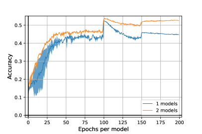
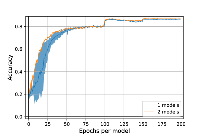
In this subsection, we experimentally investigate the effect of the regularization. In Figure 4, we notice, that the regularization has the effect of stabilizing, reducing the variance and improving the level of the robust accuracy for adversarial training for mixtures (Algorithm 2). The standard accuracy curves are very similar in both cases.

Refer to caption
Refer to caption
Refer to caption
Refer to caption
Figure 4: On left and middle-left: Standard accuracies over epochs with respectively no regularization and regularization set to α=0.001\alpha=0.001. On middle right and right: Robust accuracies for the same parameters against PGD attack with 2020 iterations and ε=0.03\varepsilon=0.03.

D.3 Additional Experiments on WideResNet28x10

We now evaluate our algorithm on WideResNet28x10 [42] architecture. Due to computation costs, we limit ourselves to 11 and 22 models, with regularization parameter set to 0.0010.001 as in the paper experiments section. Results are reported in Figure 5. We remark this architecture can lead to more robust models, corroborating the results from [19].

Models Acc. APGDCE\textrm{APGD}_{\textrm{CE}} APGDDLR\textrm{APGD}_{\textrm{DLR}} Rob. Acc.
1 85.2%85.2\% 49.9%49.9\% 50.2%50.2\% 48.5%48.5\%
2 86.0%\bm{86.0\%} 51.5%\bm{51.5\%} 52.1%\bm{52.1\%} 49.6%\bm{49.6\%}
Refer to captionRefer to caption
Figure 5: On left: Comparison of our algorithm with a standard adversarial training (one model) on WideResNet28x10. We reported the results for the model with the best robust accuracy obtained over two independent runs because adversarial training might be unstable. Standard and Robust accuracy (respectively in the middle and on right) on CIFAR-10 test images in function of the number of epochs per classifier with 11 and 22 WideResNet28x10 models. The performed attack is PGD with 2020 iterations and ε=8/255\varepsilon=8/255.

D.4 Overfitting in Adversarial Robustness

We further investigate the overfitting of our heuristic algorithm. We plotted in Figure 6 the robust accuracy on ResNet18 with 11 to 55 models. The most robust mixture of 55 models against PGD with 2020 iterations arrives at epoch 198198, i.e. at the end of the training, contrary to 11 to 44 models, where the most robust mixture occurs around epoch 101101. However, the accuracy against AGPD with 100 iterations in lower than the one at epoch 101101 with global robust accuracy of 47.6%47.6\% at epoch 101101 and 45.3%45.3\% at epoch 198. This strange phenomenon would suggest that the more powerful the attacks are, the more the models are subject to overfitting. We leave this question to further works.

Refer to caption
Refer to caption
Figure 6: Standard and Robust accuracy (respectively on left and on right) on CIFAR-10 test images in function of the number of epochs per classifier with 11 to 55 ResNet18 models. The performed attack is PGD with 2020 iterations and ε=8/255\varepsilon=8/255. The best mixture for 55 models occurs at the end of training (epoch 198198).

Appendix E Additional Results

E.1 Equality of Standard Randomized and Deterministic Minimal Risks

Proposition 7.

Let \mathbb{P} be a Borel probability distribution on 𝒳×𝒴\mathcal{X}\times\mathcal{Y}, and ll a loss satisfying Assumption 1, then:

infμ+1(Θ)(μ)=infθΘ(θ)\displaystyle\inf_{\mu\in\mathcal{M}^{1}_{+}(\Theta)}\mathcal{R}(\mu)=\inf_{\theta\in\Theta}\mathcal{R}(\theta)
Proof.

It is clear that: infμ+1(Θ)(μ)infθΘ(θ)\inf_{\mu\in\mathcal{M}^{1}_{+}(\Theta)}\mathcal{R}(\mu)\leq\inf_{\theta\in\Theta}\mathcal{R}(\theta). Now, let μ+1(Θ)\mu\in\mathcal{M}^{1}_{+}(\Theta), then:

(μ)=𝔼θμ((θ))\displaystyle\mathcal{R}(\mu)=\mathbb{E}_{\theta\sim\mu}(\mathcal{R}(\theta)) essinfμ𝔼θμ((θ))\displaystyle\geq\operatorname*{essinf}_{\mu}\mathbb{E}_{\theta\sim\mu}\left(\mathcal{R}(\theta)\right)
infθΘ(θ).\displaystyle\geq\inf_{\theta\in\Theta}\mathcal{R}(\theta).

where essinf\operatorname*{essinf} denotes the essential infimum. ∎

We can deduce an immediate corollary.

Corollary 2.

Under Assumption 1, the dual for randomized and deterministic classifiers are equal.

E.2 Decomposition of the Empirical Risk for Entropic Regularization

Proposition 8.

Let ^:=1Ni=1Nδ(xi,yi)\hat{\mathbb{P}}:=\frac{1}{N}\sum_{i=1}^{N}\delta_{(x_{i},y_{i})}. Let ll be a loss satisfying Assumption 1. Then we have:

1Ni=1Nsupx,d(x,xi)ε𝔼θμ[l(θ,(x,y))]=i=1NsupiΓi,ε𝔼(x,y)i,θμ[l(θ,(x,y))]\displaystyle\frac{1}{N}\sum_{i=1}^{N}\sup_{x,~{}d(x,x_{i})\leq\varepsilon}\mathbb{E}_{\theta\sim\mu}\left[l(\theta,(x,y))\right]=\sum_{i=1}^{N}\sup_{\mathbb{Q}_{i}\in\Gamma_{i,\varepsilon}}\mathbb{E}_{(x,y)\sim\mathbb{Q}_{i},\theta\sim\mu}\left[l(\theta,(x,y))\right]

where Γi,ε\Gamma_{i,\varepsilon} is defined as :

Γi,ε:={i𝑑i=1N,cε((xi,yi),)𝑑i=0}.\displaystyle\Gamma_{i,\varepsilon}:=\Big{\{}\mathbb{Q}_{i}\mid~{}\int d\mathbb{Q}_{i}=\frac{1}{N},~{}\int c_{\varepsilon}((x_{i},y_{i}),\cdot)d\mathbb{Q}_{i}=0\Big{\}}.
Proof.

This proposition is a direct application of Proposition 2 for diracs δ(xi,yi)\delta_{(x_{i},y_{i})}. ∎

E.3 On the NP-Hardness of Attacking a Mixture of Classifiers

In general, the problem of finding a best response to a mixture of classifiers is in general NP-hard. Let us justify it on a mixture of linear classifiers in binary classification: fθk(x)=θ,xf_{\theta_{k}}(x)=\langle\theta,x\rangle for k[L]k\in[L] and 𝝀=𝟏L/L\bm{\lambda}=\mathbf{1}_{L}/L. Let us consider the 2\ell_{2} norm and x=0x=0 and y=1y=1. Then the problem of attacking xx is the following:

supτ,τε1Lk=1L𝟏θk,τ0\displaystyle\sup_{\tau,~{}\lVert\tau\rVert\leq\varepsilon}\frac{1}{L}\sum_{k=1}^{L}\mathbf{1}_{\langle\theta_{k},\tau\rangle\leq 0}

This problem is equivalent to a linear binary classification problem on τ\tau, which is known to be NP-hard.

E.4 Case of Separated Conditional Distribtions

Proposition 9.

Let 𝒴={1,+1}\mathcal{Y}=\{-1,+1\}. Let +1(𝒳×𝒴)\mathbb{P}\in\mathcal{M}^{1}_{+}(\mathcal{X}\times\mathcal{Y}). Let ε>0\varepsilon>0. For i𝒴i\in\mathcal{Y}, let us denote i\mathbb{P}_{i} the distribution of \mathbb{P} conditionally to y=iy=i. Let us assume that d𝒳(supp(1+1),supp(1))>2εd_{\mathcal{X}}(\operatorname*{supp}(\mathbb{P}_{1+1}),\operatorname*{supp}(\mathbb{P}_{-1}))>2\varepsilon. Let us consider the nearest neighbor deterministic classifier : f(x)=d(x,supp(+1))d(x,supp(1))f(x)=d(x,\operatorname*{supp}(\mathbb{P}_{+1}))-d(x,\operatorname*{supp}(\mathbb{P}_{-1})) and the 0/10/1 loss l(f,(x,y))=𝟏yf(x)0l(f,(x,y))=\mathbf{1}_{yf(x)\leq 0}. Then ff satisfies both optimal standard and adversarial risks: (f)=0\mathcal{R}(f)=0 and advε(f)=0\mathcal{R}_{adv}^{\varepsilon}(f)=0.

Proof.

Let Let denote pi=(y=i)p_{i}=\mathbb{P}(y=i). Then we have

advε(f)=p+1𝔼+1[supx,d(x,x)ε𝟏f(x)0]+p1𝔼1[supx,d(x,x)ε𝟏f(x)0]\displaystyle\mathcal{R}_{adv}^{\varepsilon}(f)=p_{+1}\mathbb{E}_{\mathbb{P}_{+1}}\left[\sup_{x^{\prime},~{}d(x,x^{\prime})\leq\varepsilon}\mathbf{1}_{f(x^{\prime})\leq 0}\right]+p_{-1}\mathbb{E}_{\mathbb{P}_{-1}}\left[\sup_{x^{\prime},~{}d(x,x^{\prime})\leq\varepsilon}\mathbf{1}_{f(x^{\prime})\geq 0}\right]

For xsupp(+1)x\in\operatorname*{supp}(\mathbb{P}_{+1}), we have, for all xx^{\prime} such that d(x,x)0d(x,x^{\prime})\neq 0, f(x)>0f(x^{\prime})>0, then: 𝔼+1[supx,d(x,x)ε𝟏f(x)0]=0\mathbb{E}_{\mathbb{P}_{+1}}\left[\sup_{x^{\prime},~{}d(x,x^{\prime})\leq\varepsilon}\mathbf{1}_{f(x^{\prime})\leq 0}\right]=0. Similarly, we have 𝔼1[supx,d(x,x)ε𝟏f(x)0]=0\mathbb{E}_{\mathbb{P}_{-1}}\left[\sup_{x^{\prime},~{}d(x,x^{\prime})\leq\varepsilon}\mathbf{1}_{f(x^{\prime})\geq 0}\right]=0. We then deduce the result. ∎