This paper was converted on www.awesomepapers.org from LaTeX by an anonymous user.
Want to know more? Visit the Converter page.

Mixed-permutation channel with its application to estimate quantum coherence

Lin Zhang1111E-mail: godyalin@163.com and Ming-Jing Zhao2222E-mail: zhaomingjingde@126.com
1
Institute of Mathematics, Hangzhou Dianzi University, Hangzhou 310018, PR China
2School of Science, Beijing Information Science and Technology University, Beijing, 100192, PR China
Abstract

Quantum channel, as the information transmitter, is an indispensable tool in quantum information theory. In this paper, we study a class of special quantum channels named the mixed-permutation channels. The properties of these channels are characterized. The mixed-permutation channels can be applied to give a lower bound of quantum coherence with respect to any coherence measure. In particular, the analytical lower bounds for l1l_{1}-norm coherence and the relative entropy of coherence are shown respectively. The extension to bipartite systems is presented for the actions of the mixed-permutation channels.

1 Introduction

Quantum channel is a deterministic quantum operation and it transmits the information from the input to the output. It is indispensable in various information processing tasks, such as quantum communication [1], quantum computation [2, 3] and quantum cryptography [4, 5]. So the study about quantum channel is an interesting and attractive topic. Explicitly, the resource theory of quantum channels deals with understanding the properties and capabilities of quantum channels in terms of the resources they consume and produce [6, 7, 8, 9, 10, 11]. It also has important implications for the design of quantum protocols, as it provides a unified framework [12] for characterizing the capabilities and limitations of different types of quantum channels. For quantum channels, the uncertainty relations, a fundamental topic in quantum mechanics, are also established recently. They describe the theoretical restrictions about two or more quantum channels [13, 14, 15], just like that about two or more observables. In addition, quantum channels are also intimately related to the dynamical behavior of quantum states and the investigation of open quantum system [16, 17, 18].

One special kind of the most commonly-used quantum channels is the projective measurement. Within the framework of the projective measurement, many quantum features are manifested. For instance, quantum coherence is such a quantum feature and it is of practical significance in quantum computation and quantum communication [19, 20, 21]. The quantum coherence is further quantified by coherence measures such as the l1l_{1}-norm coherence [22], the relative entropy of coherence [22], the coherence concurrence [23], the geometric coherence [24] and the robustness of coherence [25] and so on. However, the evaluation of the coherence measure is not always easy for arbitrary quantum states, especially for mixed states.

In this paper, we investigate an interesting quantum channel called the mixed-permutation channel, which maps an input state to an average of their permutation conjugations. This mixed-permutation channel can be viewed as a special mixed-unitary channels with equal weights [26]. More than that, it is also an example of a covariant quantum channel [27], meaning that it commutes with certain symmetry operations on the input states. In this case, this mixed-permutation channel is covariant with respect to the conjugated action of the symmetric group SdS_{d}.

This work is factually a follow-up study of [28], which investigates the application of the mixed-permutation channel in quantifying quantum coherence. Here we aim to explore the mixed-permutation channel further and characterize it systematically. Moreover, we find the application of the mixed-permutation channel to evaluate the quantum coherence. This evaluation is applicable to all coherence measures and is tight for some special quantum states.

The paper is organized as follows. In Sect. 2, we give the definition of the mixed-permutation channels and list their basic properties. We also present the specific form of the mixed-permutation channels, and characterize the image states. The applications of the mixed-permutation channel in estimating quantum coherence is also presented. Subsequently, in Sect. 3, we extend the action of the mixed-permutation channels to bipartite systems. We conclude this paper in Sect. 4.

2 Mixed-permutation channel and its application in estimating quantum coherence

In this section, we consider the dd-dimensional quantum system with its Hilbert space d\mathbb{C}^{d} and fix the reference basis as {|i}i=1d\{|i\rangle\}_{i=1}^{d}. The so-called quantum state is represented by the density matrices/operators acting on the Hilbert space d\mathbb{C}^{d}. We denote the set of all density matrices by

D(d)={ρ=i,j=1dρij|ij|:ρ0,Tr(ρ)=1}.\mathrm{D}\left(\mathbb{C}^{d}\right)=\left\{\rho=\sum^{d}_{i,j=1}\rho_{ij}|i\rangle\langle j|:\rho\geqslant 0,\operatorname{Tr}\left(\rho\right)=1\right\}.

Any quantum channel Λ\Lambda acting on the density matrices/operators in D(d)\mathrm{D}\left(\mathbb{C}^{d}\right) can be expressed with Kraus representation Λ()=μKμ()Kμ\Lambda(\cdot)=\sum_{\mu}K_{\mu}(\cdot)K_{\mu}^{\dagger} where μKμKμ=𝟙d\sum_{\mu}K_{\mu}^{\dagger}K_{\mu}=\mathbb{1}_{d}, the identity operator on d\mathbb{C}^{d}. Next we shall introduce the mixed-permutation channels and characterize it both analytically and geometrically. Then we explain its application in estimating quantum coherence.

2.1 Mixed-permutation channels

Definition 1.

For any matrix 𝑶\boldsymbol{O} acting on d\mathbb{C}^{d}, we define the mixed-permutation channel Δ\Delta as

Δ(𝑶):=1d!πSd𝑷π𝑶𝑷π,\displaystyle\Delta(\boldsymbol{O}):=\frac{1}{d!}\sum_{\pi\in S_{d}}\boldsymbol{P}_{\pi}\boldsymbol{O}\boldsymbol{P}^{\dagger}_{\pi}, (1)

where SdS_{d} is the symmetric group of permutations of dd elements, and the permutation matrix 𝑷π\boldsymbol{P}_{\pi} is

𝑷π=i=1d|π(i)i|.\displaystyle\boldsymbol{P}_{\pi}=\sum^{d}_{i=1}|\pi(i)\rangle\langle i|. (2)

induced by πSd\pi\in S_{d}.

By this definition we see for any matrix 𝑶\boldsymbol{O} acting on d\mathbb{C}^{d}, the action of the mixed-permutation channel is the average action over all possible permutation matrices. It is easily seen that 𝑷π𝑷σ=𝑷πσ\boldsymbol{P}_{\pi}\boldsymbol{P}_{\sigma}=\boldsymbol{P}_{\pi\sigma} and 𝑷π=𝑷π𝖳=𝑷π1\boldsymbol{P}^{\dagger}_{\pi}=\boldsymbol{P}^{\scriptscriptstyle\mathsf{T}}_{\pi}=\boldsymbol{P}_{\pi^{-1}} for any π\pi and σ\sigma in SdS_{d}. Moreover, Δ(𝑶)=1d!πSd𝑷π𝑶𝑷π\Delta(\boldsymbol{O})=\frac{1}{d!}\sum_{\pi\in S_{d}}\boldsymbol{P}^{\dagger}_{\pi}\boldsymbol{O}\boldsymbol{P}_{\pi}. The properties of the mixed-permutation channel Δ\Delta can be listed below:

  1. (i)

    ΔΔ=Δ\Delta\circ\Delta=\Delta, that is ΔΔ(𝑶)=Δ(𝑶)\Delta\circ\Delta(\boldsymbol{O})=\Delta(\boldsymbol{O}) for any matrix 𝑶\boldsymbol{O} acting on d\mathbb{C}^{d}.

  2. (ii)

    Δ\Delta is unital, that is Δ(𝟙d)=𝟙d\Delta(\mathbb{1}_{d})=\mathbb{1}_{d}, where 𝟙d\mathbb{1}_{d} is the identity matrix on d\mathbb{C}^{d}.

  3. (iii)

    Δ\Delta is self-adjoint with respect to Hilbert-Schmidt inner product, i.e., Δ=Δ\Delta=\Delta^{\dagger} in the sense of Δ(𝑿),𝒀=𝑿,Δ(𝒀)\left\langle\Delta^{\dagger}(\boldsymbol{X}),\boldsymbol{Y}\right\rangle=\left\langle\boldsymbol{X},\Delta(\boldsymbol{Y})\right\rangle for all matrices 𝑿,𝒀\boldsymbol{X},\boldsymbol{Y} acting on d\mathbb{C}^{d}, that is, Δ(𝑶)=1d!πSd𝑷π𝑶𝑷π=Δ(𝑶)\Delta^{\dagger}(\boldsymbol{O})=\frac{1}{d!}\sum_{\pi\in S_{d}}\boldsymbol{P}^{\dagger}_{\pi}\boldsymbol{O}\boldsymbol{P}_{\pi}=\Delta(\boldsymbol{O}).

  4. (iv)

    [Δ(𝑶)]𝖳=Δ(𝑶𝖳)[\Delta(\boldsymbol{O})]^{\scriptscriptstyle\mathsf{T}}=\Delta(\boldsymbol{O}^{{\scriptscriptstyle\mathsf{T}}}), that is [Δ(𝑶)]𝖳=(1d!πSd𝑷π𝑶𝑷π)𝖳=1d!πSd𝑷π𝑶𝖳𝑷π=Δ(𝑶𝖳)[\Delta(\boldsymbol{O})]^{\scriptscriptstyle\mathsf{T}}=(\frac{1}{d!}\sum_{\pi\in S_{d}}\boldsymbol{P}_{\pi}\boldsymbol{O}\boldsymbol{P}^{\dagger}_{\pi})^{\scriptscriptstyle\mathsf{T}}=\frac{1}{d!}\sum_{\pi\in S_{d}}\boldsymbol{P}_{\pi}\boldsymbol{O}^{\scriptscriptstyle\mathsf{T}}\boldsymbol{P}^{\dagger}_{\pi}=\Delta(\boldsymbol{O}^{{\scriptscriptstyle\mathsf{T}}}).

  5. (v)

    Δ\Delta is invariant under any permutation matrices, that is, 𝑷τΔ(𝑶)𝑷τ=Δ(𝑶)\boldsymbol{P}_{\tau}\Delta(\boldsymbol{O})\boldsymbol{P}^{\dagger}_{\tau}=\Delta(\boldsymbol{O}) for any permutation matrix 𝑷τ\boldsymbol{P}_{\tau}, induced by the permutation τSd\tau\in S_{d}.

Furthermore, the explicit form of the mixed-permutation channel on the d\mathbb{C}^{d} can be obtained analytically.

Theorem 1.

For any d×dd\times d matrix 𝐎=(oij)\boldsymbol{O}=(o_{ij}), the mixed-permutation channel can be characterized as

Δ(𝑶)=Tr(𝑶)𝟙dd+Tr(𝑶(𝑬𝟙d))(𝑬𝟙d)d(d1),\displaystyle\Delta(\boldsymbol{O})=\operatorname{Tr}\left(\boldsymbol{O}\right)\frac{\mathbb{1}_{d}}{d}+\operatorname{Tr}\left(\boldsymbol{O}(\boldsymbol{E}-\mathbb{1}_{d})\right)\frac{(\boldsymbol{E}-\mathbb{1}_{d})}{d(d-1)}, (3)

where 𝐄:=|𝐞𝐞|\boldsymbol{E}:=|\boldsymbol{e}\rangle\!\langle\boldsymbol{e}| for dd-dimensional vector 𝐞=(1,1,,1)𝖳\boldsymbol{e}=(1,1,\ldots,1)^{\scriptscriptstyle\mathsf{T}} with all entries being one.

Proof.

In fact, this result will be established by linearity once we show it holds for any Hermitian matrix 𝑶\boldsymbol{O} because every complex square matrix 𝑴\boldsymbol{M} can be represented as a complex linear combination of two Hermitian matrices, i.e., 𝑴=𝑯+i𝑲\boldsymbol{M}=\boldsymbol{H}+\mathrm{i}\boldsymbol{K}, where 𝑯:=𝑴+𝑴2\boldsymbol{H}:=\frac{\boldsymbol{M}+\boldsymbol{M}^{\dagger}}{2} and 𝑲=𝑴𝑴2i\boldsymbol{K}=\frac{\boldsymbol{M}-\boldsymbol{M}^{\dagger}}{2\mathrm{i}}. In what follows, it suffices to consider Hermitian case.

Let us assume that 𝑶\boldsymbol{O} is Hermitian. If iji\neq j, then

i|Δ(𝑶)|j\displaystyle\left\langle i\left|\Delta(\boldsymbol{O})\right|j\right\rangle =\displaystyle= 1d!πSdi|𝑷π𝑶𝑷π|j=1d!πSdπ(i)|𝑶|π(j)=1d!πSdoπ(i)π(j).\displaystyle\frac{1}{d!}\sum_{\pi\in S_{d}}\left\langle i\left|\boldsymbol{P}^{\dagger}_{\pi}\boldsymbol{O}\boldsymbol{P}_{\pi}\right|j\right\rangle=\frac{1}{d!}\sum_{\pi\in S_{d}}\left\langle\pi(i)\left|\boldsymbol{O}\right|\pi(j)\right\rangle=\frac{1}{d!}\sum_{\pi\in S_{d}}o_{\pi(i)\pi(j)}.

Now there exists a permutation τ0Sd\tau_{0}\in S_{d} such that i=τ0(1)i=\tau_{0}(1) and j=τ0(2)j=\tau_{0}(2) due to the assumption iji\neq j. Then

πSdoπ(i)π(j)=πSdoπτ0(1)πτ0(2)=πSdoπ(1)π(2),\displaystyle\sum_{\pi\in S_{d}}o_{\pi(i)\pi(j)}=\sum_{\pi\in S_{d}}o_{\pi\tau_{0}(1)\pi\tau_{0}(2)}=\sum_{\pi\in S_{d}}o_{\pi(1)\pi(2)},

implying that, whenever iji\neq j, then

i|Δ(𝑶)|j=1|Δ(𝑶)|2.\displaystyle\left\langle i\left|\Delta(\boldsymbol{O})\right|j\right\rangle=\left\langle 1\left|\Delta(\boldsymbol{O})\right|2\right\rangle.

Similarly, if i=ji=j, then

i|Δ(𝑶)|i=1d!πSdoπ(i)π(i)=1d!πSdoπ(1)π(1)=1|Δ(𝑶)|1.\displaystyle\left\langle i\left|\Delta(\boldsymbol{O})\right|i\right\rangle=\frac{1}{d!}\sum_{\pi\in S_{d}}o_{\pi(i)\pi(i)}=\frac{1}{d!}\sum_{\pi\in S_{d}}o_{\pi(1)\pi(1)}=\left\langle 1\left|\Delta(\boldsymbol{O})\right|1\right\rangle.

Note that Tr(𝑶)=Tr(Δ(𝑶))=i=1di|Δ(𝑶)|i=d1|Δ(𝑶)|1\operatorname{Tr}\left(\boldsymbol{O}\right)=\operatorname{Tr}\left(\Delta(\boldsymbol{O})\right)=\sum^{d}_{i=1}\left\langle i\left|\Delta(\boldsymbol{O})\right|i\right\rangle=d\left\langle 1\left|\Delta(\boldsymbol{O})\right|1\right\rangle, which means that

i|Δ(𝑶)|i=Tr(𝑶)d.\displaystyle\left\langle i\left|\Delta(\boldsymbol{O})\right|i\right\rangle=\frac{\operatorname{Tr}\left(\boldsymbol{O}\right)}{d}.

From the above discussion, let 𝑬:=|𝒆𝒆|\boldsymbol{E}:=|\boldsymbol{e}\rangle\!\langle\boldsymbol{e}|, where 𝒆=(1,,1)𝖳\boldsymbol{e}=(1,\ldots,1)^{\scriptscriptstyle\mathsf{T}}. We see that

Δ(𝑶)=Tr(𝑶)d𝟙d+ζ(𝑬𝟙d).\displaystyle\Delta(\boldsymbol{O})=\frac{\operatorname{Tr}\left(\boldsymbol{O}\right)}{d}\mathbb{1}_{d}+\zeta(\boldsymbol{E}-\mathbb{1}_{d}).

Then, via 𝑬2=d𝑬\boldsymbol{E}^{2}=d\cdot\boldsymbol{E},

𝑬Δ(𝑶)𝑬=Tr(𝑶)d𝑬2+ζ(𝑬3𝑬2)=[Tr(𝑶)+ζd(d1)]𝑬.\displaystyle\boldsymbol{E}\Delta(\boldsymbol{O})\boldsymbol{E}=\frac{\operatorname{Tr}\left(\boldsymbol{O}\right)}{d}\boldsymbol{E}^{2}+\zeta(\boldsymbol{E}^{3}-\boldsymbol{E}^{2})=[\operatorname{Tr}\left(\boldsymbol{O}\right)+\zeta d(d-1)]\boldsymbol{E}.

Because 𝑷π𝑬=𝑬\boldsymbol{P}_{\pi}\boldsymbol{E}=\boldsymbol{E}, we get that 𝑬Δ(𝑶)𝑬=𝑬𝑶𝑬=𝒆|𝑶|𝒆𝑬\boldsymbol{E}\Delta(\boldsymbol{O})\boldsymbol{E}=\boldsymbol{E}\boldsymbol{O}\boldsymbol{E}=\left\langle\boldsymbol{e}\left|\boldsymbol{O}\right|\boldsymbol{e}\right\rangle\boldsymbol{E}. From these, we see that

𝒆|𝑶|𝒆=Tr(𝑶)+ζd(d1),\displaystyle\left\langle\boldsymbol{e}\left|\boldsymbol{O}\right|\boldsymbol{e}\right\rangle=\operatorname{Tr}\left(\boldsymbol{O}\right)+\zeta d(d-1),

from which we get

ζ=𝒆|𝑶|𝒆Tr(𝑶)d(d1)=2Re(oij)d(d1)=(d2)1Re(oij).\displaystyle\zeta=\frac{\left\langle\boldsymbol{e}\left|\boldsymbol{O}\right|\boldsymbol{e}\right\rangle-\operatorname{Tr}\left(\boldsymbol{O}\right)}{d(d-1)}=\frac{2\mathrm{Re}(o_{ij})}{d(d-1)}=\binom{d}{2}^{-1}\mathrm{Re}(o_{ij}).

Therefore

Δ(𝑶)\displaystyle\Delta(\boldsymbol{O}) =\displaystyle= Tr(𝑶)d𝟙d+ζ(𝑬𝟙d)\displaystyle\frac{\operatorname{Tr}\left(\boldsymbol{O}\right)}{d}\mathbb{1}_{d}+\zeta(\boldsymbol{E}-\mathbb{1}_{d})
=\displaystyle= Tr(𝑶)d𝟙d+𝒆|𝑶|𝒆Tr(𝑶)d(d1)(𝑬𝟙d)\displaystyle\frac{\operatorname{Tr}\left(\boldsymbol{O}\right)}{d}\mathbb{1}_{d}+\frac{\left\langle\boldsymbol{e}\left|\boldsymbol{O}\right|\boldsymbol{e}\right\rangle-\operatorname{Tr}\left(\boldsymbol{O}\right)}{d(d-1)}(\boldsymbol{E}-\mathbb{1}_{d})
=\displaystyle= Tr(𝑶)d𝟙d+Tr(𝑶𝑬)Tr(𝑶)d(d1)(𝑬𝟙d).\displaystyle\frac{\operatorname{Tr}\left(\boldsymbol{O}\right)}{d}\mathbb{1}_{d}+\frac{\operatorname{Tr}\left(\boldsymbol{O}\boldsymbol{E}\right)-\operatorname{Tr}\left(\boldsymbol{O}\right)}{d(d-1)}(\boldsymbol{E}-\mathbb{1}_{d}).

After simplifying it then we get the desired expression. This completes the proof. ∎

In Theorem 1, when 𝑶\boldsymbol{O} is taken as a quantum state ρD(d)\rho\in\mathrm{D}\left(\mathbb{C}^{d}\right), i.e., if a quantum state ρ\rho goes through the mixed-permutation channel Δ\Delta, then the output state Δ(ρ)\Delta(\rho) can be characterized analytically.

Corollary 1.

For any quantum state ρ=i,j=1dρij|ij|D(d)\rho=\sum^{d}_{i,j=1}\rho_{ij}|i\rangle\langle j|\in\mathrm{D}\left(\mathbb{C}^{d}\right), the corresponding output state ρ:=Δ(ρ)\rho_{\star}:=\Delta(\rho) from the mixed-permutation channel is given by

ρ=(d1𝔞𝔞𝔞d1𝔞𝔞𝔞d1),\displaystyle\rho_{\star}=\left(\begin{array}[]{cccccccc}d^{-1}&\mathfrak{a}&\cdots&\mathfrak{a}\\ \mathfrak{a}&d^{-1}&\cdots&\mathfrak{a}\\ \vdots&\vdots&\ddots&\vdots\\ \mathfrak{a}&\mathfrak{a}&\cdots&d^{-1}\end{array}\right), (8)

where

𝔞:=1d(d1)ijρij\displaystyle\mathfrak{a}:=\frac{1}{d(d-1)}\sum_{i\neq j}\rho_{ij} (9)

for the given reference basis {|i:1,,d}\{|i\rangle:1,\ldots,d\}.

Remark 1.

We remark here that 𝔞[1d(d1),1d]\mathfrak{a}\in\left[-\frac{1}{d(d-1)},\frac{1}{d}\right]. Indeed,

ijρij=i,j=1dρij1=Tr(ρ𝑬)1=𝒆|ρ|𝒆1.\displaystyle\sum_{i\neq j}\rho_{ij}=\sum_{i,j=1}^{d}\rho_{ij}-1=\operatorname{Tr}\left(\rho\boldsymbol{E}\right)-1=\left\langle\boldsymbol{e}\left|\rho\right|\boldsymbol{e}\right\rangle-1.

Therefore, combining dλmin(ρ)𝒆|ρ|𝒆dλmax(ρ)d\lambda_{\min}(\rho)\leqslant\left\langle\boldsymbol{e}\left|\rho\right|\boldsymbol{e}\right\rangle\leqslant d\lambda_{\max}(\rho), where λmin(ρ)\lambda_{\min}(\rho) and λmax(ρ)\lambda_{\max}(\rho) are the minimum and maximum eigenvalues of the quantum state ρ\rho respectively, we have,

1d(d1)dλmin(ρ)1d(d1)𝔞=1d(d1)ijρijdλmax(ρ)1d(d1)1d.\displaystyle-\frac{1}{d(d-1)}\leqslant\frac{d\lambda_{\min}(\rho)-1}{d(d-1)}\leqslant\mathfrak{a}=\frac{1}{d(d-1)}\sum_{i\neq j}\rho_{ij}\leqslant\frac{d\lambda_{\max}(\rho)-1}{d(d-1)}\leqslant\frac{1}{d}. (10)

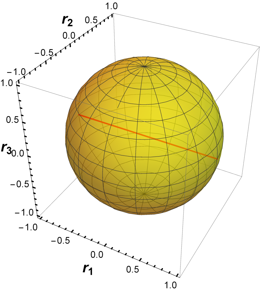
In order to see clearly what is the image states Δ(ρ)\Delta(\rho) of the channel Δ\Delta when input state is ρ\rho, let us focus on qubit systems. In fact, any qubit state can be represented as

ρ=12(𝟙2+𝒓𝝈)=12(1+r3r1ir2r1+ir21r3),\displaystyle\rho=\frac{1}{2}(\mathbb{1}_{2}+\boldsymbol{r}\cdot\boldsymbol{\sigma})=\frac{1}{2}\left(\begin{array}[]{cc}1+r_{3}&r_{1}-\mathrm{i}r_{2}\\ r_{1}+\mathrm{i}r_{2}&1-r_{3}\end{array}\right), (13)

where rir_{i}\in\mathbb{R}, r:=|𝒓|=r12+r22+r321r:=\left\lvert\mspace{1.0mu}\boldsymbol{r}\mspace{1.0mu}\right\rvert=\sqrt{r_{1}^{2}+r_{2}^{2}+r_{3}^{2}}\leqslant 1, and 𝒓𝝈:=k=13rkσk\boldsymbol{r}\cdot\boldsymbol{\sigma}:=\sum^{3}_{k=1}r_{k}\sigma_{k}, 𝝈:=(σ1,σ2,σ3)\boldsymbol{\sigma}:=(\sigma_{1},\sigma_{2},\sigma_{3}) is the vector of the Pauli matrices, given by

σ1=(0110),σ2=(0ii0),σ3=(1001).\displaystyle\sigma_{1}=\left(\begin{array}[]{cc}0&1\\ 1&0\end{array}\right),\quad\sigma_{2}=\left(\begin{array}[]{cc}0&-\mathrm{i}\\ \mathrm{i}&0\end{array}\right),\quad\sigma_{3}=\left(\begin{array}[]{cc}1&0\\ 0&-1\end{array}\right). (20)

It is easily seen that the action of Δ\Delta is

Δ(ρ)=12(𝟙2+𝒓𝝈)=12(1r1r11).\displaystyle\Delta(\rho)=\frac{1}{2}(\mathbb{1}_{2}+\boldsymbol{r}^{\prime}\cdot\boldsymbol{\sigma})=\frac{1}{2}\left(\begin{array}[]{cc}1&r_{1}\\ r_{1}&1\end{array}\right). (23)

So the action of the mixed-permutation channel on the set of quantum states can be simulated by the transformation on the Bloch ball, i.e.,

𝒓=(r1,r2,r3)𝒓=(r1,0,0).\displaystyle\boldsymbol{r}=(r_{1},r_{2},r_{3})\rightarrow\boldsymbol{r}^{\prime}=(r_{1},0,0). (24)

From Figure 1, we see that the Bloch ball is mapped into a red line segment by the action of the mixed-permutation channel.

Refer to caption
Figure 1: (Color Online) The whole yellow Bloch ball stands for the family of all qubit states in Eq. (13); the red line segment stands for the image states Δ(ρ)\Delta(\rho) in Eq. (23) when qubit states ρ\rho through the mixed-permutation channel.

2.2 Applying the mixed-permutation channel to estimate quantum coherence

In order to estimate quantum coherence using the mixed-permutation channel, we need recall some notions about quantum coherence. Given the reference basis {|i}i=1d\{|i\rangle\}_{i=1}^{d}, a diagonal quantum state ϱ=i=1dλi|ii|\varrho=\sum_{i=1}^{d}\lambda_{i}|i\rangle\!\langle i| is called the incoherent state. The set of incoherent states is denoted as \mathcal{I}. The so-called incoherent operation is a completely positive linear mapping Φ\Phi such that its Kraus decomposition Φ(ρ)=νKνρKν\Phi(\rho)=\sum_{\nu}K_{\nu}\rho K_{\nu}^{\dagger} with νKνKν=𝟙\sum_{\nu}K_{\nu}^{\dagger}K_{\nu}=\mathbb{1} fulfills KνδKν/Tr(KνδKν)K_{\nu}\delta K_{\nu}^{\dagger}/\operatorname{Tr}\left(K_{\nu}\delta K_{\nu}^{\dagger}\right)\in\mathcal{I} for all δ\delta\in\mathcal{I} and for all ν\nu.

The quantum coherence is quantified by a nonnegative function named the coherence measure. A coherence measure is required to satisfy the following conditions [22]:

  1. (A1)

    Nonnegativity: C(ρ)0C(\rho)\geqslant 0 for ρD(d)\rho\in\mathrm{D}\left(\mathbb{C}^{d}\right), and moreover C(ρ)=0C(\rho)=0 for all ρ\rho\in\mathcal{I};

  2. (A2)

    Monotonicity: C(Φ(ρ))C(ρ)C(\Phi(\rho))\leqslant C(\rho) for any incoherent operation Φ\Phi;

  3. (A3)

    Strong monotonicity: νpνC(KνρKν/pν)C(ρ)\sum_{\nu}p_{\nu}C(K_{\nu}\rho K_{\nu}^{\dagger}/p_{\nu})\leqslant C(\rho) for any incoherent operation Φ(ρ)=νKνρKν\Phi(\rho)=\sum_{\nu}K_{\nu}\rho K_{\nu}^{\dagger} with pν=Tr(KνρKν)p_{\nu}=\operatorname{Tr}\left(K_{\nu}\rho K_{\nu}^{\dagger}\right) and ρν=KνρKν/pν\rho_{\nu}=K_{\nu}\rho K_{\nu}^{\dagger}/p_{\nu};

  4. (A4)

    Convexity: C(ρ)kpkC(ρk)C(\rho)\leqslant\sum_{k}p_{k}C(\rho_{k}) for any quantum state ρ=kpkρk\rho=\sum_{k}p_{k}\rho_{k} with pk0p_{k}\geqslant 0 and kpk=1\sum_{k}p_{k}=1.

Two commonly used coherence measures are the l1l_{1}-norm coherence and the relative entropy of coherence [22]. The l1l_{1}-norm coherence of the quantum state ρ=i,jρij|ij|\rho=\sum_{i,j}\rho_{ij}|i\rangle\langle j| is the sum of the magnitudes of all the off-diagonal entries

Cl1(ρ):=ij|ρij|.\displaystyle C_{l_{1}}(\rho):=\sum_{i\neq j}\left\lvert\mspace{1.0mu}\rho_{ij}\mspace{1.0mu}\right\rvert. (25)

The relative entropy of coherence is the difference of von Neumann entropy between the density matrix and the diagonal matrix given by its diagonal entries,

Cr(ρ):=S(Π(ρ))S(ρ),\displaystyle C_{r}(\rho):=S(\Pi(\rho))-S(\rho), (26)

where Π(ρ)=diag(ρ11,ρ22,,ρdd)\Pi(\rho)=\mathrm{diag}(\rho_{11},\rho_{22},\cdots,\rho_{dd}) is the diagonal matrix obtained by the diagonal entries of ρ\rho and S(ρ):=Tr(ρlnρ)S(\rho):=-\operatorname{Tr}\left(\rho\ln\rho\right) is the von Neumann entropy of the state ρ\rho.

Now we come back to the mixed-permutation channel. It is obvious that 𝑷πρ𝑷π\boldsymbol{P}_{\pi}\rho\boldsymbol{P}^{\dagger}_{\pi} is incoherent for any incoherent state ρ\rho. So the mixed-permutation channel is an incoherent operation. By the monotonicity of the coherence measures, we know the coherence of input state ρ\rho is nonincreasing under this channel. Since the output states of the mixed-permutation channel have an analytical form ρ\rho_{\star} in Eq. (8), we can utilize it to estimate the coherence of the input state ρ\rho.

Theorem 2.

For any coherence measure CC and any quantum state ρD(d)\rho\in\mathrm{D}\left(\mathbb{C}^{d}\right), the quantum coherence of ρ\rho is bounded from below by the quantum coherence of ρ\rho_{\star}, namely,

C(ρ)C(ρ).\displaystyle C(\rho)\geqslant C(\rho_{\star}). (27)
Proof.

First, since any permutation matrices 𝑷π\boldsymbol{P}_{\pi} and 𝑷π1\boldsymbol{P}_{\pi^{-1}} are incoherent operations, so

C(ρ)=C[𝑷π(𝑷πρ𝑷π)𝑷π]C(𝑷πρ𝑷π)C(ρ).C(\rho)=C[\boldsymbol{P}^{\dagger}_{\pi}(\boldsymbol{P}_{\pi}\rho\boldsymbol{P}^{\dagger}_{\pi})\boldsymbol{P}_{\pi}]\leqslant C(\boldsymbol{P}_{\pi}\rho\boldsymbol{P}^{\dagger}_{\pi})\leqslant C(\rho).

Therefore C(𝑷πρ𝑷π)=C(ρ)C(\boldsymbol{P}_{\pi}\rho\boldsymbol{P}^{\dagger}_{\pi})=C(\rho) for any permutation matrcix 𝑷π\boldsymbol{P}_{\pi}. Then by the convexity of coherence measure, we have further that

C(ρ)=C(Δ(ρ))\displaystyle C(\rho_{\star})=C(\Delta(\rho)) =\displaystyle= C(1d!πSd𝑷πρ𝑷π)\displaystyle C\left(\frac{1}{d!}\sum_{\pi\in S_{d}}\boldsymbol{P}_{\pi}\rho\boldsymbol{P}^{\dagger}_{\pi}\right)
\displaystyle\leqslant 1d!πSdC(𝑷πρ𝑷π)\displaystyle\frac{1}{d!}\sum_{\pi\in S_{d}}C\left(\boldsymbol{P}_{\pi}\rho\boldsymbol{P}^{\dagger}_{\pi}\right)
=\displaystyle= 1d!πSdC(ρ)\displaystyle\frac{1}{d!}\sum_{\pi\in S_{d}}C(\rho)
=\displaystyle= C(ρ),\displaystyle C(\rho),

which completes the proof. ∎

From the proof above, we see that Theorem 2 is universal in the sense that Eq. (30) is independent of the coherence measures. So Theorem 2 can be applied to all coherence measures. Additionally, the output states ρ\rho_{\star} is of one parameter, so its coherence is much easy to calculate compared with the input state. In fact, for any quantum state ρ=i,j=1dρij|ij|\rho=\sum^{d}_{i,j=1}\rho_{ij}|i\rangle\langle j|, the output state ρ\rho_{\star} in Corollary 1 can be decomposed as

ρ=(1𝔭)𝟙d/d+𝔭|ΦdΦd|,\displaystyle\rho_{\star}=(1-\mathfrak{p})\mathbb{1}_{d}/d+\mathfrak{p}|\Phi_{d}\rangle\!\langle\Phi_{d}|, (28)

where the weight is relevant to the quantum state as

𝔭:=1d1ijρij[1d1,1]\displaystyle\mathfrak{p}:=\frac{1}{d-1}\sum_{i\neq j}\rho_{ij}\in\left[-\frac{1}{d-1},1\right] (29)

and |Φd:=1di=1d|i|\Phi_{d}\rangle:=\frac{1}{\sqrt{d}}\sum^{d}_{i=1}|i\rangle is the maximally coherent state [29]. This state ρ\rho_{\star} is also called the maximally coherent mixed state in [30]. By this decomposition in Eq. (28), we get the eigenvalues of ρ\rho_{\star} is 𝔭+1𝔭d\mathfrak{p}+\frac{1-\mathfrak{p}}{d} and (1𝔭)/d(1-\mathfrak{p})/d with multiplicity d1d-1. In view of this, we get the following result:

Corollary 2.

For any quantum state ρD(d)\rho\in\mathrm{D}\left(\mathbb{C}^{d}\right), the l1l_{1}-norm coherence and the relative entropy of coherence can be valuated from below by

Cl1(ρ)\displaystyle C_{l_{1}}(\rho) \displaystyle\geqslant d(d1)|𝔞|,\displaystyle d(d-1)\left\lvert\mspace{1.0mu}\mathfrak{a}\mspace{1.0mu}\right\rvert, (30)
Cr(ρ)\displaystyle C_{r}(\rho) \displaystyle\geqslant (11d)(1𝔭)ln(1𝔭)+1d[(d1)𝔭+1]ln[(d1)𝔭+1],\displaystyle\left(1-\frac{1}{d}\right)(1-\mathfrak{p})\ln(1-\mathfrak{p})+\frac{1}{d}[(d-1)\mathfrak{p}+1]\ln[(d-1)\mathfrak{p}+1], (31)

respectively, where 𝔞\mathfrak{a} and 𝔭\mathfrak{p} are depended by ρ\rho as Eqs. (9) and (29).

For l1l_{1} norm coherence, the lower bound in Eq. (30) is tight for real quantum states, that is,

Cl1(ρ)=Cl1(ρ)\displaystyle C_{l_{1}}(\rho)=C_{l_{1}}(\rho_{\star}) (32)

for any real quantum state ρ\rho. Now we consider the l1l_{1}-norm coherence and the relative entropy of coherence in qubit system.
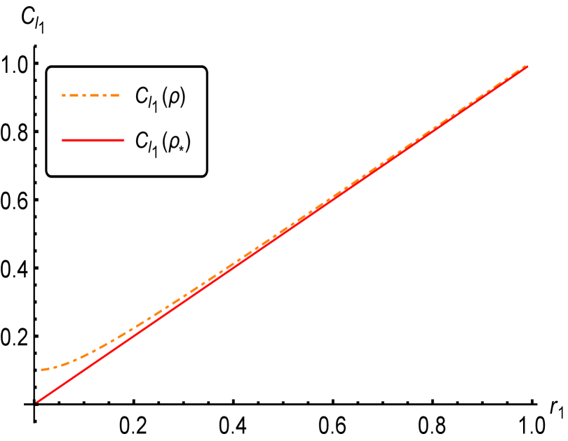
Example 1.

In qubit systems, any qubit state ρ\rho can be represented as in Eq. (13) with the spectral decomposition as

ρ=λ1|ϕ1ϕ1|+λ2|ϕ2ϕ2|\rho=\lambda_{1}|\phi_{1}\rangle\!\langle\phi_{1}|+\lambda_{2}|\phi_{2}\rangle\!\langle\phi_{2}|

with the eigenvalues λ1=12(1+r)\lambda_{1}=\frac{1}{2}(1+r), λ2=12(1r)\lambda_{2}=\frac{1}{2}(1-r) and the corresponding eigenvectors

|ϕ1=(r1ir2)|0(r3r)|12r(rr3),|ϕ2=(r1ir2)|0(r3+r)|12r(r+r3).|\phi_{1}\rangle=\frac{(r_{1}-\mathrm{i}r_{2})|0\rangle-(r_{3}-r)|1\rangle}{\sqrt{2r(r-r_{3})}},\quad|\phi_{2}\rangle=\frac{(r_{1}-\mathrm{i}r_{2})|0\rangle-(r_{3}+r)|1\rangle}{\sqrt{2r(r+r_{3})}}.

Let r2=r3=110r_{2}=r_{3}=\frac{1}{10}, we calculate the l1l_{1}-norm coherence Cl1(ρ)C_{l_{1}}(\rho) and the relative entropy coherence Cr(ρ)C_{r}(\rho) as well as the lower bound the l1l_{1}-norm coherence Cl1(ρ)C_{l_{1}}(\rho_{\star}) and the relative entropy coherence Cr(ρ)C_{r}(\rho_{\star}) and make a comparison in Figures 2 and 2.

Refer to caption
Refer to caption
Figure 2: (Color Online) The estimation of the coherence of ρ\rho by that of ρ\rho_{\star} using the l1l_{1}-norm coherence measure in subfigure (a) and the relative entropy of coherence in subfigure (b).

From another point of view, it is interesting to estimate quantum coherence from above. Let us turn to another quantity called the coherence of assistance, induced by any coherence measure CC, which is defined in the form of concave bottom extension,

Ca(ρ)=maxkpkC(|ψk),\displaystyle C_{a}(\rho)=\max\sum_{k}p_{k}C(|\psi_{k}\rangle), (33)

where the maximization is taken over all pure state decompositions of ρ=kpk|ψkψk|\rho=\sum_{k}p_{k}|\psi_{k}\rangle\!\langle\psi_{k}|. Coherence of assistance quantifies the coherence that can be extracted assisted by another party under local measurements and classical communication [31]. Suppose Alice holds a state ρA=ρ=kpk|ψkψk|\rho^{A}=\rho=\sum_{k}p_{k}|\psi_{k}\rangle\!\langle\psi_{k}| with coherence C(ρ)C(\rho). Bob holds another part of the purified state of ρ\rho. The joint state between Alice and Bob is kpk|ψkA|kB\sum_{k}p_{k}|\psi_{k}\rangle_{A}\otimes|k\rangle_{B}. Bob performs local projective measurements {|kk|}\left\{|k\rangle\!\langle k|\right\} along the given basis and informs Alice the measurement outcomes by classical communication. Alice’s system will be in a pure state ensemble {pk,|ψkψk|}\left\{p_{k},|\psi_{k}\rangle\!\langle\psi_{k}|\right\} with average coherence kpkC(|ψkψk|)\sum_{k}p_{k}C(|\psi_{k}\rangle\!\langle\psi_{k}|). The process is called assisted coherence distillation. The maximum average coherence is called the coherence of assistance which quantifies the one-way coherence distillation rate [31].

The coherence of assistance of any quantum state ρ\rho can be estimated by the output state ρ=Δ(ρ)\rho_{\star}=\Delta(\rho).

Theorem 3.

For any coherence measure CC and any quantum state ρD(d)\rho\in\mathrm{D}\left(\mathbb{C}^{d}\right), the coherence of assistance of ρ\rho is bounded from above by the coherence of assistance of ρ=Δ(ρ)\rho_{\star}=\Delta(\rho),

Ca(ρ)Ca(ρ).\displaystyle C_{a}(\rho)\leqslant C_{a}(\rho_{\star}). (34)
Proof.

Note that

Ca(ρ)\displaystyle C_{a}(\rho_{\star}) =\displaystyle= Ca(Δ(ρ))\displaystyle C_{a}(\Delta(\rho))
=\displaystyle= Ca(1d!πSd𝑷πρ𝑷π)\displaystyle C_{a}\left(\frac{1}{d!}\sum_{\pi\in S_{d}}\boldsymbol{P}_{\pi}\rho\boldsymbol{P}^{\dagger}_{\pi}\right)
\displaystyle\geqslant 1d!πSdCa(𝑷πρ𝑷π)\displaystyle\frac{1}{d!}\sum_{\pi\in S_{d}}C_{a}(\boldsymbol{P}_{\pi}\rho\boldsymbol{P}^{\dagger}_{\pi})
=\displaystyle= Ca(ρ).\displaystyle C_{a}(\rho).

Here the inequality is the concavity of the coherence of assistance. The last equality is due to the equality Ca(𝑷πρ𝑷π)=Ca(ρ)C_{a}(\boldsymbol{P}_{\pi}\rho\boldsymbol{P}^{\dagger}_{\pi})=C_{a}(\rho) for any permutation πSd\pi\in S_{d}. ∎

3 Mixed-permutation channel on bipartite systems

In this section we study the mixed-permutation channel on bipartite systems dAdB\mathbb{C}^{d_{A}}\otimes\mathbb{C}^{d_{B}}. Without loss of generality, we suppose dAdBd_{A}\leqslant d_{B}. Suppose that {|i}i=1dA\{|i\rangle\}^{d_{A}}_{i=1} and {|j}j=1dB\{|j\rangle\}^{d_{B}}_{j=1} are rothonormal bases of the subsystems dA\mathbb{C}^{d_{A}} and dB\mathbb{C}^{d_{B}}, respectively, we denote by

D(dAdB)={ρAB=i,i=1dAj,j=1dBρij,ij|ijij|:ρAB0,Tr(ρAB)=1}\mathrm{D}\left(\mathbb{C}^{d_{A}}\otimes\mathbb{C}^{d_{B}}\right)=\left\{\rho_{AB}=\sum^{d_{A}}_{i,i^{\prime}=1}\sum^{d_{B}}_{j,j^{\prime}=1}\rho_{i^{\prime}j^{\prime},ij}|i^{\prime}j^{\prime}\rangle\langle ij|:\rho_{AB}\geqslant 0,\operatorname{Tr}\left(\rho_{AB}\right)=1\right\}

the set of density operators acting on dAdB\mathbb{C}^{d_{A}}\otimes\mathbb{C}^{d_{B}}. The identical channel on operator spaces are denoted by id\mathrm{id}. By Theorem 1, we derive the explicit form of the mixed-permutation channel on bipartite systems dAdB\mathbb{C}^{d_{A}}\otimes\mathbb{C}^{d_{B}}.

Theorem 4.

For any bipartite operator 𝐗AB\boldsymbol{X}_{AB} acting on dAdB\mathbb{C}^{d_{A}}\otimes\mathbb{C}^{d_{B}}, denote 𝐄A(B)=|𝐞A(B)𝐞A(B)|\boldsymbol{E}_{A(B)}=|\boldsymbol{e}_{A(B)}\rangle\!\langle\boldsymbol{e}_{A(B)}| where 𝐞A(B)\boldsymbol{e}_{A(B)} is a dA(B)d_{A(B)}-dimensional column vector with all entries being one, we have

(ΔAidB)(𝑿AB)=𝟙AdATrA(𝑿AB)+𝑬A𝟙AdA(dA1)TrA(𝑿AB(𝑬A𝟙A)𝟙B)\displaystyle(\Delta_{A}\otimes\mathrm{id}_{B})(\boldsymbol{X}_{AB})=\frac{\mathbb{1}_{A}}{d_{A}}\otimes\operatorname{Tr}_{A}\left(\boldsymbol{X}_{AB}\right)+\frac{\boldsymbol{E}_{A}-\mathbb{1}_{A}}{d_{A}(d_{A}-1)}\otimes\operatorname{Tr}_{A}\left(\boldsymbol{X}_{AB}(\boldsymbol{E}_{A}-\mathbb{1}_{A})\otimes\mathbb{1}_{B}\right) (35)

and thus

(ΔAΔB)(𝑿AB)\displaystyle(\Delta_{A}\otimes\Delta_{B})(\boldsymbol{X}_{AB}) =\displaystyle= c0(𝑿AB)𝟙AB+c1(𝑿AB)𝟙A(𝑬B𝟙B)+c2(𝑿AB)(𝑬A𝟙A)𝟙B\displaystyle c_{0}(\boldsymbol{X}_{AB})\mathbb{1}_{AB}+c_{1}(\boldsymbol{X}_{AB})\mathbb{1}_{A}\otimes(\boldsymbol{E}_{B}-\mathbb{1}_{B})+c_{2}(\boldsymbol{X}_{AB})(\boldsymbol{E}_{A}-\mathbb{1}_{A})\otimes\mathbb{1}_{B} (36)
+c3(𝑿AB)(𝑬A𝟙A)(𝑬B𝟙B).\displaystyle+c_{3}(\boldsymbol{X}_{AB})(\boldsymbol{E}_{A}-\mathbb{1}_{A})\otimes(\boldsymbol{E}_{B}-\mathbb{1}_{B}).

where

{c0(𝑿AB)=1dAdBTr(𝑿AB),c1(𝑿AB)=1dAdB(dB1)Tr(𝑿AB(𝑬A𝟙A)𝟙B),c2(𝑿AB)=1dAdB(dA1)Tr(𝑿AB𝟙A(𝑬B𝟙B)),c3(𝑿AB)=1dAdB(dA1)(dB1)Tr(𝑿AB(𝑬A𝟙A)(𝑬B𝟙B)).\displaystyle\begin{cases}c_{0}(\boldsymbol{X}_{AB})=\frac{1}{d_{A}d_{B}}\operatorname{Tr}\left(\boldsymbol{X}_{AB}\right),\\ c_{1}(\boldsymbol{X}_{AB})=\frac{1}{d_{A}d_{B}(d_{B}-1)}\operatorname{Tr}\left(\boldsymbol{X}_{AB}(\boldsymbol{E}_{A}-\mathbb{1}_{A})\otimes\mathbb{1}_{B}\right),\\ c_{2}(\boldsymbol{X}_{AB})=\frac{1}{d_{A}d_{B}(d_{A}-1)}\operatorname{Tr}\left(\boldsymbol{X}_{AB}\mathbb{1}_{A}\otimes(\boldsymbol{E}_{B}-\mathbb{1}_{B})\right),\\ c_{3}(\boldsymbol{X}_{AB})=\frac{1}{d_{A}d_{B}(d_{A}-1)(d_{B}-1)}\operatorname{Tr}\left(\boldsymbol{X}_{AB}(\boldsymbol{E}_{A}-\mathbb{1}_{A})\otimes(\boldsymbol{E}_{B}-\mathbb{1}_{B})\right).\end{cases} (37)
Proof.

The result can be also established by linearity once we show it holds for any Hermitian matrix 𝑿AB\boldsymbol{X}_{AB}. So it suffices to consider the Hermitian case.

  1. (i)

    In fact, for 𝑿AB=|ΨABΨAB|\boldsymbol{X}_{AB}=|\Psi_{AB}\rangle\!\langle\Psi_{AB}| where |ΨABdAdB|\Psi_{AB}\rangle\in\mathbb{C}^{d_{A}}\otimes\mathbb{C}^{d_{B}}, we suppose its Schmidt decomposition is

    |ΨAB=i=1dAλi|𝒂iA|𝒃iB,|\Psi_{AB}\rangle=\sum_{i=1}^{d_{A}}\sqrt{\lambda_{i}}|\boldsymbol{a}_{i}\rangle_{A}\otimes|\boldsymbol{b}_{i}\rangle_{B},

    with {|𝒂iA}i=1dA\{|\boldsymbol{a}_{i}\rangle_{A}\}_{i=1}^{d_{A}} and {|𝒃jB}j=1dB\{|\boldsymbol{b}_{j}\rangle_{B}\}_{j=1}^{d_{B}} the orthnormal bases of the subsystems dA\mathbb{C}^{d_{A}} and dB\mathbb{C}^{d_{B}} respectively, then the density operator of |ΨABΨAB||\Psi_{AB}\rangle\!\langle\Psi_{AB}| can be expressed as

    |ΨABΨAB|=i,j=1dAλiλj|𝒂i𝒂j|A|𝒃i𝒃j|B.|\Psi_{AB}\rangle\!\langle\Psi_{AB}|=\sum_{i,j=1}^{d_{A}}\sqrt{\lambda_{i}\lambda_{j}}|\boldsymbol{a}_{i}\rangle\langle\boldsymbol{a}_{j}|_{A}\otimes|\boldsymbol{b}_{i}\rangle\langle\boldsymbol{b}_{j}|_{B}.

    In the following reasoning, we omit the subindexes AA and BB when no confusing arises. The action of the mixed-permutation channel on the first subsystem is then

    (ΔAidB)(|ΨABΨAB|)\displaystyle(\Delta_{A}\otimes\mathrm{id}_{B})(|\Psi_{AB}\rangle\!\langle\Psi_{AB}|)
    =\displaystyle= i,j=1dAλiλjΔA(|𝒂i𝒂j|)|𝒃i𝒃j|\displaystyle\sum_{i,j=1}^{d_{A}}\sqrt{\lambda_{i}\lambda_{j}}\Delta_{A}(|\boldsymbol{a}_{i}\rangle\langle\boldsymbol{a}_{j}|)\otimes|\boldsymbol{b}_{i}\rangle\langle\boldsymbol{b}_{j}|
    =\displaystyle= i,j=1dAλiλj[Tr(|𝒂i𝒂j|)𝟙dAdA+Tr(|𝒂i𝒂j|(𝑬A𝟙dA))(𝑬A𝟙dA)dA(dA1)]|𝒃i𝒃j|\displaystyle\sum_{i,j=1}^{d_{A}}\sqrt{\lambda_{i}\lambda_{j}}\left[\operatorname{Tr}\left(|\boldsymbol{a}_{i}\rangle\langle\boldsymbol{a}_{j}|\right)\frac{\mathbb{1}_{d_{A}}}{d_{A}}+\operatorname{Tr}\left(|\boldsymbol{a}_{i}\rangle\langle\boldsymbol{a}_{j}|(\boldsymbol{E}_{A}-\mathbb{1}_{d_{A}})\right)\frac{(\boldsymbol{E}_{A}-\mathbb{1}_{d_{A}})}{d_{A}(d_{A}-1)}\right]\otimes|\boldsymbol{b}_{i}\rangle\langle\boldsymbol{b}_{j}|
    =\displaystyle= 𝟙dAdA(i,j=1dAλiλjTr(|𝒂i𝒂j|)|𝒃i𝒃j|)\displaystyle\frac{\mathbb{1}_{d_{A}}}{d_{A}}\otimes\left(\sum_{i,j=1}^{d_{A}}\sqrt{\lambda_{i}\lambda_{j}}\operatorname{Tr}\left(|\boldsymbol{a}_{i}\rangle\langle\boldsymbol{a}_{j}|\right)|\boldsymbol{b}_{i}\rangle\langle\boldsymbol{b}_{j}|\right)
    +(𝑬A𝟙dA)dA(dA1)(i,j=1dAλiλjTr(|𝒂i𝒂j|(𝑬A𝟙dA))|𝒃i𝒃j|)\displaystyle+\frac{(\boldsymbol{E}_{A}-\mathbb{1}_{d_{A}})}{d_{A}(d_{A}-1)}\otimes\left(\sum_{i,j=1}^{d_{A}}\sqrt{\lambda_{i}\lambda_{j}}\operatorname{Tr}\left(|\boldsymbol{a}_{i}\rangle\langle\boldsymbol{a}_{j}|(\boldsymbol{E}_{A}-\mathbb{1}_{d_{A}})\right)|\boldsymbol{b}_{i}\rangle\langle\boldsymbol{b}_{j}|\right)
    =\displaystyle= 𝟙dAdATrA(|ΨABΨAB|)+(𝑬A𝟙dA)dA(dA1)TrA(|ΨABΨAB|(𝑬A𝟙dA)𝟙dB).\displaystyle\frac{\mathbb{1}_{d_{A}}}{d_{A}}\otimes\operatorname{Tr}_{A}(|\Psi_{AB}\rangle\!\langle\Psi_{AB}|)+\frac{(\boldsymbol{E}_{A}-\mathbb{1}_{d_{A}})}{d_{A}(d_{A}-1)}\otimes\operatorname{Tr}_{A}(|\Psi_{AB}\rangle\!\langle\Psi_{AB}|(\boldsymbol{E}_{A}-\mathbb{1}_{d_{A}})\otimes\mathbb{1}_{d_{B}}).

    By the linearity of both sides, this equality holds for any positive semi-definite bipartite operator, and thus for a general bipartite operator.

  2. (ii)

    The proof goes similarly.

We have done the proof. ∎

If we focus on the bipartite quantum states, then we get an output state of the one-sided and two-sided mixed-permutation channels as follows.

Corollary 3.

For any quantum state ρABD(dAdB)\rho_{AB}\in\mathrm{D}\left(\mathbb{C}^{d_{A}}\otimes\mathbb{C}^{d_{B}}\right), if the first subsystem goes through the mixed-permutation channel, then the output state is

(ΔAidB)(ρAB)=𝟙dAdAρB+dA|ΦdAΦdA|𝟙dAdA(dA1)TrA(ρAB(dA|ΦdAΦdA|𝟙dA)𝟙dB),\displaystyle(\Delta_{A}\otimes\mathrm{id}_{B})(\rho_{AB})=\frac{\mathbb{1}_{d_{A}}}{d_{A}}\otimes\rho_{B}+\frac{d_{A}|\Phi_{d_{A}}\rangle\!\langle\Phi_{d_{A}}|-\mathbb{1}_{d_{A}}}{d_{A}(d_{A}-1)}\otimes\operatorname{Tr}_{A}\left(\rho_{AB}(d_{A}|\Phi_{d_{A}}\rangle\!\langle\Phi_{d_{A}}|-\mathbb{1}_{d_{A}})\otimes\mathbb{1}_{d_{B}}\right), (38)

where ρB=TrA(ρAB)\rho_{B}=\operatorname{Tr}_{A}(\rho_{AB}). If both subsystems go through the separate mixed-permutation channels, the output state is

(ΔAΔB)(ρAB)\displaystyle(\Delta_{A}\otimes\Delta_{B})(\rho_{AB}) =\displaystyle= 𝟙dAdA𝟙dBdB+γ1(ρAB)𝟙dAdAdB|ΦdBΦdB|𝟙dBdB(dB1)\displaystyle\frac{\mathbb{1}_{d_{A}}}{d_{A}}\otimes\frac{\mathbb{1}_{d_{B}}}{d_{B}}+\gamma_{1}(\rho_{AB})\frac{\mathbb{1}_{d_{A}}}{d_{A}}\otimes\frac{d_{B}|\Phi_{d_{B}}\rangle\!\langle\Phi_{d_{B}}|-\mathbb{1}_{d_{B}}}{d_{B}(d_{B}-1)}
+γ2(ρAB)dA|ΦdAΦdA|𝟙dAdA(dA1)𝟙BdB\displaystyle+\gamma_{2}(\rho_{AB})\frac{d_{A}|\Phi_{d_{A}}\rangle\!\langle\Phi_{d_{A}}|-\mathbb{1}_{d_{A}}}{d_{A}(d_{A}-1)}\otimes\frac{\mathbb{1}_{B}}{d_{B}}
+γ3(ρAB)dA|ΦdAΦdA|𝟙AdA(dA1)dB|ΦdBΦdB|𝟙dBdB(dB1).\displaystyle+\gamma_{3}(\rho_{AB})\frac{d_{A}|\Phi_{d_{A}}\rangle\!\langle\Phi_{d_{A}}|-\mathbb{1}_{A}}{d_{A}(d_{A}-1)}\otimes\frac{d_{B}|\Phi_{d_{B}}\rangle\!\langle\Phi_{d_{B}}|-\mathbb{1}_{d_{B}}}{d_{B}(d_{B}-1)}.

Here |ΦdA=1dAi=1dA|𝐚i|\Phi_{d_{A}}\rangle=\frac{1}{\sqrt{d_{A}}}\sum_{i=1}^{d_{A}}|\boldsymbol{a}_{i}\rangle and |ΦdB=1dBj=1dB|𝐛j|\Phi_{d_{B}}\rangle=\frac{1}{\sqrt{d_{B}}}\sum_{j=1}^{d_{B}}|\boldsymbol{b}_{j}\rangle. Moreover,

γ1(ρAB)\displaystyle\gamma_{1}(\rho_{AB}) :=\displaystyle:= Tr(ρAB(dA|ΦdAΦdA|𝟙dA)𝟙dB),\displaystyle\operatorname{Tr}\left(\rho_{AB}(d_{A}|\Phi_{d_{A}}\rangle\!\langle\Phi_{d_{A}}|-\mathbb{1}_{d_{A}})\otimes\mathbb{1}_{d_{B}}\right),
γ2(ρAB)\displaystyle\gamma_{2}(\rho_{AB}) :=\displaystyle:= Tr(ρAB𝟙dA(dB|ΦdBΦdB|𝟙dB)),\displaystyle\operatorname{Tr}\left(\rho_{AB}\mathbb{1}_{d_{A}}\otimes(d_{B}|\Phi_{d_{B}}\rangle\!\langle\Phi_{d_{B}}|-\mathbb{1}_{d_{B}})\right),
γ3(ρAB)\displaystyle\gamma_{3}(\rho_{AB}) :=\displaystyle:= Tr(ρAB(dA|ΦdAΦdA|𝟙dA)(dB|ΦdBΦdB|𝟙dB)).\displaystyle\operatorname{Tr}\left(\rho_{AB}(d_{A}|\Phi_{d_{A}}\rangle\!\langle\Phi_{d_{A}}|-\mathbb{1}_{d_{A}})\otimes(d_{B}|\Phi_{d_{B}}\rangle\!\langle\Phi_{d_{B}}|-\mathbb{1}_{d_{B}})\right).

By the form of the output states (ΔAidB)(ρAB)(\Delta_{A}\otimes\mathrm{id}_{B})(\rho_{AB}) and (ΔAΔB)(ρAB)(\Delta_{A}\otimes\Delta_{B})(\rho_{AB}) in the above Corollary 3, we get both (ΔAidB)(ρAB)(\Delta_{A}\otimes\mathrm{id}_{B})(\rho_{AB}) and (ΔAΔB)(ρAB)(\Delta_{A}\otimes\Delta_{B})(\rho_{AB}) are positive under partial transpositions (PPT) for all states ρAB\rho_{AB}. Since PPT states in qubit-qubit systems and qubit-qutrit systems are all separable, so the action of the local mixed-permutation channel(s) on two-qubit systems will completely erase the entanglement between two subsystems.

Example 2.

For any quantum state ρAB\rho_{AB} in D(22)\mathrm{D}\left(\mathbb{C}^{2}\otimes\mathbb{C}^{2}\right),

ρAB=(ρ11ρ12ρ13ρ14ρ21ρ22ρ23ρ24ρ31ρ32ρ33ρ34ρ41ρ42ρ43ρ44),\rho_{AB}=\left(\begin{array}[]{cccc}\rho_{11}&\rho_{12}&\rho_{13}&\rho_{14}\\ \rho_{21}&\rho_{22}&\rho_{23}&\rho_{24}\\ \rho_{31}&\rho_{32}&\rho_{33}&\rho_{34}\\ \rho_{41}&\rho_{42}&\rho_{43}&\rho_{44}\end{array}\right),

if the first qubit goes through the mixed-permutation channel, then the output state is

(ρAB),I=(ΔAidB)(ρAB)=𝟙dAdAρB+𝑬A𝟙dAdA(dA1)TrA(ρAB(𝑬A𝟙dA)𝟙dB),\displaystyle(\rho_{AB})_{\star,I}=(\Delta_{A}\otimes\mathrm{id}_{B})(\rho_{AB})=\frac{\mathbb{1}_{d_{A}}}{d_{A}}\otimes\rho_{B}+\frac{\boldsymbol{E}_{A}-\mathbb{1}_{d_{A}}}{d_{A}(d_{A}-1)}\otimes\operatorname{Tr}_{A}\left(\rho_{AB}(\boldsymbol{E}_{A}-\mathbb{1}_{d_{A}})\otimes\mathbb{1}_{d_{B}}\right), (39)

with

ρB=TrA(ρAB)=(ρ11+ρ22ρ13+ρ24ρ31+ρ42ρ33+ρ44).\rho_{B}=\operatorname{Tr}_{A}(\rho_{AB})=\left(\begin{array}[]{cc}\rho_{11}+\rho_{22}&\rho_{13}+\rho_{24}\\ \rho_{31}+\rho_{42}&\rho_{33}+\rho_{44}\end{array}\right).

More explicitly,

(ρAB),I=(ρ11+ρ22ρ12+ρ21ρ13+ρ24ρ14+ρ23ρ12+ρ21ρ11+ρ22ρ14+ρ23ρ13+ρ24ρ31+ρ42ρ32+ρ41ρ33+ρ44ρ34+ρ43ρ32+ρ41ρ31+ρ42ρ34+ρ43ρ33+ρ44)\displaystyle(\rho_{AB})_{\star,I}=\left(\begin{array}[]{cccc}\rho_{11}+\rho_{22}&\rho_{12}+\rho_{21}&\rho_{13}+\rho_{24}&\rho_{14}+\rho_{23}\\ \rho_{12}+\rho_{21}&\rho_{11}+\rho_{22}&\rho_{14}+\rho_{23}&\rho_{13}+\rho_{24}\\ \rho_{31}+\rho_{42}&\rho_{32}+\rho_{41}&\rho_{33}+\rho_{44}&\rho_{34}+\rho_{43}\\ \rho_{32}+\rho_{41}&\rho_{31}+\rho_{42}&\rho_{34}+\rho_{43}&\rho_{33}+\rho_{44}\\ \end{array}\right) (44)

with (ρAB),I𝖳A=(ρAB),I(\rho_{AB})^{{\scriptscriptstyle\mathsf{T}}_{A}}_{\star,I}=(\rho_{AB})_{\star,I}. Furthermore, if both two qubits go through the mixed-permutation channel, then the output state is

(ρAB),\displaystyle(\rho_{AB})_{\star,\star} =\displaystyle= (ΔAΔB)(ρAB)\displaystyle(\Delta_{A}\otimes\Delta_{B})(\rho_{AB})
=\displaystyle= c0(ρ)𝟙dAdB+c1(ρ)𝟙dA(𝑬B𝟙dB)\displaystyle c_{0}(\rho)\mathbb{1}_{d_{A}d_{B}}+c_{1}(\rho)\mathbb{1}_{d_{A}}\otimes(\boldsymbol{E}_{B}-\mathbb{1}_{d_{B}})
+c2(ρ)(𝑬A𝟙dA)𝟙dB+c3(ρ)(𝑬A𝟙dA)(𝑬B𝟙dB)\displaystyle+c_{2}(\rho)(\boldsymbol{E}_{A}-\mathbb{1}_{d_{A}})\otimes\mathbb{1}_{d_{B}}+c_{3}(\rho)(\boldsymbol{E}_{A}-\mathbb{1}_{d_{A}})\otimes(\boldsymbol{E}_{B}-\mathbb{1}_{d_{B}})
=\displaystyle= (c0(ρAB)c1(ρAB)c2(ρAB)c3(ρAB)c1(ρAB)c0(ρAB)c3(ρAB)c2(ρAB)c2(ρAB)c3(ρAB)c0(ρAB)c1(ρAB)c3(ρAB)c2(ρAB)c1(ρAB)c0(ρAB))=(ρAB),𝖳A0,\displaystyle\left(\begin{array}[]{cccc}c_{0}(\rho_{AB})&c_{1}(\rho_{AB})&c_{2}(\rho_{AB})&c_{3}(\rho_{AB})\\ c_{1}(\rho_{AB})&c_{0}(\rho_{AB})&c_{3}(\rho_{AB})&c_{2}(\rho_{AB})\\ c_{2}(\rho_{AB})&c_{3}(\rho_{AB})&c_{0}(\rho_{AB})&c_{1}(\rho_{AB})\\ c_{3}(\rho_{AB})&c_{2}(\rho_{AB})&c_{1}(\rho_{AB})&c_{0}(\rho_{AB})\\ \end{array}\right)=(\rho_{AB})^{{\scriptscriptstyle\mathsf{T}}_{A}}_{\star,\star}\geqslant 0,

where

c0(ρAB)\displaystyle c_{0}(\rho_{AB}) =\displaystyle= 14,\displaystyle\frac{1}{4},
c1(ρAB)\displaystyle c_{1}(\rho_{AB}) =\displaystyle= 14Tr(ρA(𝑬B𝟙dB)),\displaystyle\frac{1}{4}\operatorname{Tr}\left(\rho_{A}(\boldsymbol{E}_{B}-\mathbb{1}_{d_{B}})\right),
c2(ρAB)\displaystyle c_{2}(\rho_{AB}) =\displaystyle= 14Tr(ρB(𝑬A𝟙dA)),\displaystyle\frac{1}{4}\operatorname{Tr}\left(\rho_{B}(\boldsymbol{E}_{A}-\mathbb{1}_{d_{A}})\right),
c3(ρAB)\displaystyle c_{3}(\rho_{AB}) =\displaystyle= 14Tr(ρAB(𝑬A𝟙dA)(𝑬B𝟙dB)),\displaystyle\frac{1}{4}\operatorname{Tr}\left(\rho_{AB}(\boldsymbol{E}_{A}-\mathbb{1}_{d_{A}})\otimes(\boldsymbol{E}_{B}-\mathbb{1}_{d_{B}})\right),

implying that (ρAB),(\rho_{AB})_{\star,\star} must be separable. Moreover, the eigenvalues are given by

c0(ρAB)+c1(ρAB)±(c2(ρAB)+c3(ρAB)),c0(ρAB)c1(ρAB)±(c2(ρAB)c3(ρAB)).\displaystyle c_{0}(\rho_{AB})+c_{1}(\rho_{AB})\pm(c_{2}(\rho_{AB})+c_{3}(\rho_{AB})),\quad c_{0}(\rho_{AB})-c_{1}(\rho_{AB})\pm(c_{2}(\rho_{AB})-c_{3}(\rho_{AB})).

From the above, we see that (ρAB),I(\rho_{AB})_{\star,I} and (ρAB),(\rho_{AB})_{\star,\star} are PPT states. Thus by Peres-Horodecki criterion [32, 33], the output states (ρAB),I(\rho_{AB})_{\star,I} and (ρAB),(\rho_{AB})_{\star,\star} are separable ones for all two-qubit states ρAB\rho_{AB}.

In what follows, let us recall the notion of the entanglement-breaking channel [34]. The so-called entanglement-breaking channel 𝒯𝒯A\mathcal{T}\equiv\mathcal{T}_{A} means that (𝒯AidB)(ρAB)(\mathcal{T}_{A}\otimes\mathrm{id}_{B})(\rho_{AB}) is separable for every bipartite state ρABD(dAdB)\rho_{AB}\in\mathrm{D}\left(\mathbb{C}^{d_{A}}\otimes\mathbb{C}^{d_{B}}\right). As already known in [35], in qubit systems, any quantum channel is entanglement breaking if and only if its Choi representation is separable. Because (ΔAidB)(ρAB)(\Delta_{A}\otimes\mathrm{id}_{B})(\rho_{AB}) is separable for any two-qubit state ρAB\rho_{AB}, a fortiori for maximally entangled two-qubit state. Thus Δ\Delta is entanglement breaking in qubit systems. In fact, the mixed-permutation channel Δ\Delta is entanglement-breaking channel in qudit systems, which can be summarized into the following result:

Corollary 4.

The mixed-permutation channel Δ\Delta characterized in Theorem 1 is entanglement-breaking channel in qudit systems.

Proof.

According to [34, Theorem 4, (B)\Longleftrightarrow(C)], it suffices to show that the Choi-representation of the mixed-permutation channel Δ\Delta, J(Δ):=(Δid)(|ΩΩ|)J(\Delta):=(\Delta\otimes\mathrm{id})(|\Omega\rangle\!\langle\Omega|), is separable, where |Ω:=1di=1d|ii|\Omega\rangle:=\frac{1}{\sqrt{d}}\sum^{d}_{i=1}|ii\rangle. Indeed, using Eq. (38),

J(Δ)\displaystyle J(\Delta) =\displaystyle= 1d2𝟙d𝟙d+1d2(d1)(d|ΦdΦd|𝟙d)2\displaystyle\frac{1}{d^{2}}\mathbb{1}_{d}\otimes\mathbb{1}_{d}+\frac{1}{d^{2}(d-1)}(d|\Phi_{d}\rangle\!\langle\Phi_{d}|-\mathbb{1}_{d})^{\otimes 2}
=\displaystyle= 1d|ΦdΦd||ΦdΦd|+(11d)(𝟙d|ΦdΦd|d1)(𝟙d|ΦdΦd|d1),\displaystyle\frac{1}{d}|\Phi_{d}\rangle\!\langle\Phi_{d}|\otimes|\Phi_{d}\rangle\!\langle\Phi_{d}|+\left(1-\frac{1}{d}\right)\left(\frac{\mathbb{1}_{d}-|\Phi_{d}\rangle\!\langle\Phi_{d}|}{d-1}\right)\otimes\left(\frac{\mathbb{1}_{d}-|\Phi_{d}\rangle\!\langle\Phi_{d}|}{d-1}\right),

a separable state. Here |Φd=1di=1d|i|\Phi_{d}\rangle=\frac{1}{\sqrt{d}}\sum^{d}_{i=1}|i\rangle. This indicates that Δ\Delta is entanglement-breaking. ∎

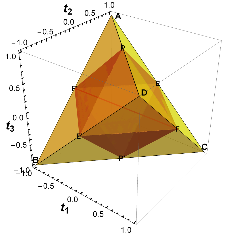
Example 3 (The family of Bell-diagonal states).

The Bell-diagonal states [36] in two-qubit system can be written as

ρBell=14(𝟙4+i=13tiσiσi)\displaystyle\rho_{\text{Bell}}=\frac{1}{4}(\mathbb{1}_{4}+\sum_{i=1}^{3}t_{i}\sigma_{i}\otimes\sigma_{i}) (46)

with σi\sigma_{i} three Pauli operators in Eq. (20). So a Bell-diagonal state is specified by three real variables t1,t2t_{1},t_{2}, and t3t_{3} such that

{1t1t2t30,1t1+t2+t30,1+t1t2+t30,1+t1+t2t30.\displaystyle\begin{cases}1-t_{1}-t_{2}-t_{3}\geqslant 0,\\ 1-t_{1}+t_{2}+t_{3}\geqslant 0,\\ 1+t_{1}-t_{2}+t_{3}\geqslant 0,\\ 1+t_{1}+t_{2}-t_{3}\geqslant 0.\end{cases}

Denote the set of all above such tuples (t1,t2,t3)(t_{1},t_{2},t_{3}) by DBellD_{\text{Bell}}. Because the four eigenvalues of ρ\rho are in [0,1][0,1], we see that ti[1,1](i=1,2,3)t_{i}\in[-1,1](i=1,2,3). That is, DBell[1,1]3D_{\text{Bell}}\subset[-1,1]^{3}. The Bell-diagonal states can be geometrically described by a tetrahedron. One can show that a Bell-diagonal state is separable if and only if |t1|+|t2|+|t3|1\left\lvert\mspace{1.0mu}t_{1}\mspace{1.0mu}\right\rvert+\left\lvert\mspace{1.0mu}t_{2}\mspace{1.0mu}\right\rvert+\left\lvert\mspace{1.0mu}t_{3}\mspace{1.0mu}\right\rvert\leqslant 1 holds. Geometrically, the set of Bell-diagonal states is a tetrahedron and the set of separable Bell-diagonal states is an octahedron [36], which is denoted by DBellsepD_{\text{Bellsep}}. That is, DBellsep={(t1,t2,t3)DBell:i=13|ti|1}D_{\text{Bellsep}}=\{(t_{1},t_{2},t_{3})\in D_{\text{Bell}}:\sum^{3}_{i=1}\left\lvert\mspace{1.0mu}t_{i}\mspace{1.0mu}\right\rvert\leqslant 1\}. We find that

Δid(ρBell)=14(𝟙4+t1σ1σ1).\displaystyle\Delta\otimes\mathrm{id}(\rho_{\mathrm{Bell}})=\frac{1}{4}(\mathbb{1}_{4}+t_{1}\sigma_{1}\otimes\sigma_{1}). (47)

We make a plot in arguments (t1,t2,t3)(t_{1},t_{2},t_{3}) about the image states in (47) of the one-sided action of the mixed-permutation channel on the family (46) of Bell diagonal states in the following Figure 3.

Refer to caption
Figure 3: (Color Online) The yellow tetrahedron stands for the family of Bell-diagonal states in Eq. (46); the orange octahedron stands for separable Bell-diagonal states; the red line segment stands for image states Δid(ρBell)\Delta\otimes\mathrm{id}(\rho_{\mathrm{Bell}}) in Eq. (47) of all diagonal Bell-diagonal states through the one-sided mixed-permutation channel.

4 Conclusions and discussions

In summary, we studied one kind of special channels, i.e., the mixed-permutation channels. The properties of this channel was characterized. The mixed-permutation channel can be used in bounding quantum coherence with respect to all coherence measures. The action of the mixed-permutation channel on bipartite systems is also discussed and can be generalized to multipartite systems. Beyond that, there are some interesting problems which can be further considered in the future:

  • The first question is what is the average collective action of the permutations on the bipartite quantum states,

    1d!πSd(𝑷π𝑷π)𝑿(𝑷π𝑷π)=?.\displaystyle\frac{1}{d!}\sum_{\pi\in S_{d}}(\boldsymbol{P}_{\pi}\otimes\boldsymbol{P}_{\pi})\boldsymbol{X}(\boldsymbol{P}_{\pi}\otimes\boldsymbol{P}_{\pi})^{\dagger}=?.

    We are expecting a closed-form formula of the above expression. With this potential formula, we can extend symmetrized variance for pure states in [28] to mixed states.

  • The second question is what is the correlation quantifiers [37] or coherence measure [38] induced by the mixed-permutation channel.

In light of the special properties and the closed form of the output state of the mixed-permutation channel, we expect the corresponding correlation measure and coherence measure could characterize the quantum features of quantum states from a permutation-invariant way.

Acknowledgments

This research is supported by Zhejiang Provincial Natural Science Foundation of China under Grant No. LZ23A010005 and by NSFC under Grant Nos.11971140 and 12171044.

Data Availability Statement

No Data associated in the manuscript.

References

  • [1] R. Takagi, K. Wang, and M. Hayashi, Application of the resource theory of channels to communication scenarios, Phys. Rev. Lett. 124, 120502 (2020).
  • [2] D.P. Divincenzo, Quantum computation, Science 270(5234), 255-261(1995).
  • [3] A. Ekert and R. Jozsa, Quantum computation and Shor’s factoring algorithm, Rev. Math. Phys. 68, 733 (1996).
  • [4] N. Gisin, G. Ribordy, W. Tittel, and H. Zbinden, Quantum cryptography, Rev. Math. Phys. 74, 145 (2002).
  • [5] S. Pirandola et al., Advances in quantum cryptography, Advances in Optics and Photonics 12(4), 1012-1236 (2020).
  • [6] E. Chitambar and G. Gour, Quantum resource theories, Rev. Math. Phys. 91, 025001 (2019).
  • [7] X. Wang and M.M. Wilde, Resource theory of asymmetric distinguishability for quantum channels, Phys. Rev. Research 1, 033169 (2019).
  • [8] X. Wang, M.M. Wilde, and Y. Su, Quantifying the magic of quantum channels, New. J. Phys. 21, 103002 (2019).
  • [9] F.H. Kamin, F.T. Tabesh, S. Salimi, and F. Kheirandish, The resource theory of coherence for quantum channels, Quant Inf Process 19, 210 (2020).
  • [10] Y. Liu and X. Yuan, Operational resource theory of quantum channels, Phys. Rev. Research 2, 012035(R) (2020).
  • [11] H. Zhou, T. Gao, F. Yan, Entanglement resource theory of quantum channel, Phys. Rev. Research 4, 013200 (2022).
  • [12] R. Takagi, Operational Quantum Resource Theories: Unified Framework and Applications, PhD Thesis (2020).
  • [13] S. Fu, Y. Sun, S. Luo, Skew information-based uncertainty relations for quantum channels, Quantum Inf. Process. 18, 258 (2019).
  • [14] N. Zhou, M. J. Zhao, Z. Wang, T. Li, The uncertainty relation for quantum channels based on skew information, Quantum Inf. Process. 22, 6 (2023).
  • [15] Q-H. Zhang, J.F. Wu, S-M. Fei, A note on uncertainty relations of arbitrary N quantum channels, Laser Phys. Lett. 18, 095204(2021).
  • [16] T.R. Bromley, M. Cianciaruso, and G. Adesso, Frozen quantum coherence, Phys. Rev. Lett. 114, 210401 (2015).
  • [17] X.D. Yu, D.J. Zhang, C.L. Liu, and D.M. Tong, Measure-independent freezing of quantum coherence, Phys. Rev. A 93, 060303 (2016).
  • [18] M.L. Hu, and H. Fan, Evolution equation for quantum coherence, Sci. Rep. 6, 29260 (2016).
  • [19] A. Streltsov, G. Adesso, and M. B. Plenio, Colloquium: Quantum coherence as a resource, Rev. Math. Phys. 89, 041003 (2017).
  • [20] E. Chitambar and G. Gour, Quantum resource theories, Rev. Math. Phys. 91, 025001 (2019).
  • [21] M.L. Hu, X. Hu, J. Wang, Y. Peng, Y.R. Zhang, H. Fan, Quantum coherence and geometric quantum discord, Phys. Rep. 762-764, 1-100 (2018).
  • [22] T. Baumgratz, M. Cramer, and M. B. Plenio, Quantifying coherence, Phys. Rev. Lett. 113, 140401 (2014).
  • [23] X. Qi, T. Gao, and F.L. Yan, Measuring coherence with entanglement concurrence, J. Phys. A 50, 285301 (2017).
  • [24] A. Streltsov, U. Singh, H. S. Dhar, M. N. Bera, and G. Adesso, Measuring Quantum Coherence with Entanglement, Phys. Rev. Lett. 115, 020403 (2015).
  • [25] C. Napoli, T. R. Bromley, M. Cianciaruso, M. Piani, N. Johnston, and G. Adesso, Robustness of coherence: an operational and observable measure of quantum coherence, Phys. Rev. Lett. 116, 150502 (2016).
  • [26] J. I de Vicente and A. Streltsov, Genuine quantum coherence, J. Phys. A: Math. Theor. 50, 045301 (2017).
  • [27] A.S. Holevo, Additive conjecture and covariant channels, Int. J. Quantum Information, 3(1),41-47 (2005).
  • [28] M. J. Zhao, L. Zhang, and S. M. Fei, Standard symmetrized variance with applications to coherence, uncertainty, and entanglement, Phys. Rev. A 106, 012417 (2022).
  • [29] Y. Peng, Y. Jiang, and H. Fan, Maximally coherent states and coherence-preserving operations, Phys. Rev. A 93, 032326 (2016).
  • [30] U. Singh, M. N. Bera, H. S. Dhar, and A. K. Pati, Maximally coherent mixed states: Complementarity between maximal coherence and mixedness, Phys. Rev. A 91, 052115 (2015).
  • [31] E. Chitambar, A. Streltsov, S. Rana, M.N. Bera, G. Adesso, and M. Lewenstein, Assisted Distillation of Quantum Coherence, Phys. Rev. Lett. 116, 070402 (2016).
  • [32] A. Peres, Separability Criterion for Density Matrices, Phys. Rev. Lett. 77, 1413 (1996).
  • [33] M. Horodecki and P. Horodecki, Reduction criterion of separability and limits for a class of distillation protocols, Phys. Rev. A 59, 4206 (1999).
  • [34] M. Horodecki, P.W. Shor, and M.B. Ruskai, Entanglement breaking channels, Rev. Math. Phys. 15(6), 629-641 (2003).
  • [35] M.B. Ruskai, Qubit entanglement breaking channels, Rev. Math. Phys. 15(6), 643(2003).
  • [36] R. Horodecki, M. Horodecki, Information-theoretic aspects of inseparability of mixed states, Phys. Rev. A 54(3), 1838 (1996).
  • [37] N. Li, S. Luo, Y. Sun, Quantifying correlations via local channels, Phys. Rev. A 105, 032436 (2022).
  • [38] Y. Sun, N. Li, S. Luo, Quantifying coherence relative to channels via metric-adjusted skew information, Phys. Rev. A  106, 012436 (2022).