Yatong Bai \Emailyatong_bai@berkeley.edu
\NameBrendon G. Anderson \Emailbganderson@berkeley.edu
\NameSomayeh Sojoudi \Emailsojoudi@berkeley.edu
\addrUniversity of California, Berkeley
Mixing Classifiers to Alleviate the Accuracy-Robustness Trade-Off
Abstract
Deep neural classifiers have recently found tremendous success in data-driven control systems. However, existing models suffer from a trade-off between accuracy and adversarial robustness. This limitation must be overcome in the control of safety-critical systems that require both high performance and rigorous robustness guarantees. In this work, we develop classifiers that simultaneously inherit high robustness from robust models and high accuracy from standard models. Specifically, we propose a theoretically motivated formulation that mixes the output probabilities of a standard neural network and a robust neural network. Both base classifiers are pre-trained, and thus our method does not require additional training. Our numerical experiments verify that the mixed classifier noticeably improves the accuracy-robustness trade-off and identify the confidence property of the robust base classifier as the key leverage of this more benign trade-off. Our theoretical results prove that under mild assumptions, when the robustness of the robust base model is certifiable, no alteration or attack within a closed-form radius on an input can result in misclassification of the mixed classifier.
keywords:
Adversarial Robustness, Image Classification, Computer Vision, Model Ensemble1 Introduction
In recent years, high-performance machine learning models have been employed in various control settings, including reinforcement learning for dynamic systems with uncertainty (Levine et al., 2016; Sutton and Barto, 2018) and autonomous driving (Bojarski et al., 2016; Wu et al., 2017). However, models such as neural networks have been shown to be vulnerable to adversarial attacks, which are imperceptibly small input data alterations maliciously designed to cause failure (Szegedy et al., 2014; Nguyen et al., 2015; Huang et al., 2017; Eykholt et al., 2018; Liu et al., 2019). This vulnerability makes such models unreliable for safety-critical control where guaranteeing robustness is necessary. In response, “adversarial training (AT)” (Kurakin et al., 2017; Goodfellow et al., 2015; Bai et al., 2022a, b; Zheng et al., 2020; Zhang et al., 2019) have been studied to alleviate the susceptibility. AT builds robust neural networks by training on adversarially attacked data.
A parallel line of work focuses on mathematically certified robustness (Anderson et al., 2020; Ma and Sojoudi, 2021; Anderson and Sojoudi, 2022a). Among these methods, “randomized smoothing (RS)” is a particularly popular one that seeks to achieve certified robustness by processing intentionally corrupted data at inference time (Cohen et al., 2019; Li et al., 2019; Pfrommer et al., 2023), and has recently been applied to robustify reinforcement learning-based control strategies (Kumar et al., 2022; Wu et al., 2022). The recent work (Anderson and Sojoudi, 2022b) has shown that “locally biased smoothing,” which robustifies the model locally based on the input test datum, outperforms the traditional RS with fixed smoothing noise. However, Anderson and Sojoudi (2022b) only focus on binary classification problems, significantly limiting the applications. Moreover, Anderson and Sojoudi (2022b) rely on the robustness of a -nearest-neighbor (-NN) classifier, which suffers from a lack of representation power when applied to harder problems and becomes a bottleneck.
While some works have shown that there exists a fundamental trade-off between accuracy and robustness (Tsipras et al., 2019; Zhang et al., 2019), recent research has argued that it should be possible to simultaneously achieve robustness and accuracy on benchmark datasets (Yang et al., 2020). To this end, variants of AT that improve the accuracy-robustness trade-off have been proposed, including TRADES (Zhang et al., 2019), Interpolated Adversarial Training (Lamb et al., 2019), and many others (Raghunathan et al., 2020; Zhang and Wang, 2019; Tramèr et al., 2018; Balaji et al., 2019). However, even with these improvements, degraded clean accuracy is often an inevitable price of achieving robustness. Moreover, standard non-robust models often achieve enormous performance gains by pre-training on larger datasets, whereas the effect of pre-training on robust classifiers is less understood and may be less prominent (Chen et al., 2020; Fan et al., 2021).
This work makes a theoretically disciplined step towards robustifying models without sacrificing clean accuracy. Specifically, we build upon locally biased smoothing and replace its underlying -NN classifier with a robust neural network that can be obtained via various existing methods. We then modify how the standard base model (a highly accurate but possibly non-robust neural network) and the robust base model are “mixed” accordingly. The resulting formulation, to be introduced in Section˜3, is a convex combination of the output probabilities from the two base classifiers. We prove that, when the robust network has a bounded Lipschitz constant or is built via RS, the mixed classifier also has a closed-form certified robust radius. More importantly, our method achieves an empirical robustness level close to that of the robust base model while approaching the standard base model’s clean accuracy. This desirable behavior significantly improves the accuracy-robustness trade-off, especially for tasks where standard models noticeably outperform robust models on clean data.
Note that we do not make any assumptions about how the standard and robust base models are obtained (can be AT, RS, or others), nor do we assume the adversarial attack type and budget. Thus, our mixed classification scheme can take advantage of pre-training on large datasets via the standard base classifier and benefit from ever-improving robust training methods via the robust base classifier.
2 Background and related works
2.1 Notations
The norm is denoted by , while denotes its dual norm. The matrix denotes the identity matrix in . For a scalar , denotes its sign. For a natural number , the set is defined as . For an event , the indicator function evaluates to 1 if takes place and 0 otherwise. The notation denotes the probability for an event to occur, where is a random variable drawn from the distribution . The normal distribution on with mean and covariance is written as . We denote the cumulative distribution function of on by and write its inverse function as .
Consider a model , whose components are , where is the dimension of the input and is the number of classes. In this paper, we assume that does not have the desired level of robustness, and refer to it as a “standard model”, as opposed to a “robust model” which we denote as . We consider norm-bounded attacks on differentiable neural networks. A classifier , defined as , is considered robust against adversarial attacks at an input datum if it assigns the same class to all perturbed inputs such that , where is the attack radius.
2.2 Related Adversarial Attacks and Defenses
The fast gradient sign method (FGSM) and projected gradient descent (PGD) attacks based on differentiating the cross-entropy loss are highly effective and have been considered the most standard attacks for evaluating robust models (Madry et al., 2018; Goodfellow et al., 2015). To exploit the structures of the defense methods, adaptive attacks have also been introduced (Tramèr et al., 2020).
On the defense side, while AT (Madry et al., 2018) and TRADES (Zhang et al., 2019) have seen enormous success, such methods are often limited by a significantly larger amount of required training data (Schmidt et al., 2018) and a decrease in generalization capability. Initiatives that construct more effective training data via data augmentation (Rebuffi et al., 2021; Gowal et al., 2021) and generative models (Sehwag et al., 2022) have successfully produced more robust models. Improved versions of AT (Jia et al., 2022; Shafahi et al., 2019) have also been proposed.
Previous initiatives that aim to enhance the accuracy-robustness trade-off include using alternative attacks during training (Pang et al., 2022), appending early-exit side branches to a single network (Hu et al., 2020), and applying AT for regularization (Zheng et al., 2021). Moreover, ensemble-based defenses, such as random ensemble (Liu et al., 2018) and diverse ensemble (Pang et al., 2019; Alam et al., 2022), have been proposed. In comparison, this work considers two separate classifiers and uses their synergy to improve the accuracy-robustness trade-off, achieving higher performances.
2.3 Locally Biased Smoothing
Randomized smoothing, popularized by (Cohen et al., 2019), achieves robustness at inference time by replacing with a smoothed classifier , where is a smoothing distribution. A common choice for is a Gaussian distribution.
Anderson and Sojoudi (2022b) have recently argued that data-invariant RS does not always achieve robustness. They have shown that in the binary classification setting, RS with an unbiased distribution is suboptimal, and an optimal smoothing procedure shifts the input point in the direction of its true class. Since the true class is generally unavailable, a “direction oracle” is used as a surrogate. This “locally biased smoothing” method is no longer randomized and outperforms traditional data-blind RS. The locally biased smoothed classifier, denoted , is obtained via the deterministic calculation , where is the direction oracle and is a trade-off parameter. The direction oracle should come from an inherently robust classifier (which is often less accurate). In (Anderson and Sojoudi, 2022b), this direction oracle is chosen to be a one-nearest-neighbor classifier.
3 Using a Robust Neural Network as the Smoothing Oracle
Locally biased smoothing was designed for binary classification, restricting its practicality. Here, we first extend it to the multi-class setting by treating the output of each class, denoted as , independently, giving rise to:
| (1) |
Note that if is large for some class , then can be large for class even if both and are small, leading to incorrect predictions. To remove the effect of the gradient magnitude difference across the classes, we propose a normalized formulation as follows:
| (2) |
The parameter adjusts between clean accuracy and robustness. It holds that when , and when for all and all .
With the mixing procedure generalized to the multi-class setting, we now discuss the choice of the smoothing oracle . While -NN classifiers are relatively robust and can be used as the oracle, their representation power is too weak. On the CIFAR-10 image classification task (Krizhevsky, 2012), -NN only achieves around accuracy on clean test data. In contrast, an adversarially trained ResNet can reach accuracy on attacked test data (Madry et al., 2018). This lackluster performance of -NN becomes a significant bottleneck in the accuracy-robustness trade-off of the mixed classifier. To this end, we replace the -NN model with a robust neural network. The robustness of this network can be achieved via various methods, including AT, TRADES, and RS.
Further scrutinizing Eq.˜2 leads to the question of whether is the best choice for adjusting the mixture of and . This gradient magnitude term is a result of Anderson and Sojoudi (2022b)’s assumption that . Here, we no longer have this assumption. Instead, we assume both and to be differentiable. Thus, we generalize the formulation to
| (3) |
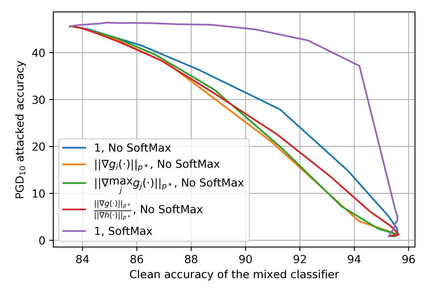
where is an extra scalar term that can potentially depend on both and to determine the “trustworthiness” of the base classifiers. Here, we empirically compare four options for , namely, , , , and .
Another design question is whether and should be the pre-softmax logits or the post-softmax probabilities. Note that since most attack methods are designed based on logits, the output of the mixed classifier should be logits rather than probabilities to avoid gradient masking, an undesirable phenomenon that makes it hard to evaluate the robustness properly. Thus, we have the following two options that make the mixed model compatible with existing gradient-based attacks:
-
1.
Use the logits for both base classifiers, and .
-
2.
Use the probabilities for both base classifiers, and then convert the mixed probabilities back to logits. The required “inverse-softmax” operator is simply the natural logarithm.
-
•
“No Softmax” represents Option 1, i.e., use the logits for and .
-
•
“Softmax” represents Option 2, i.e., use the probabilities for and .
-
•
With the best formulation, high clean accuracy can be achieved with very little sacrifice on robustness.
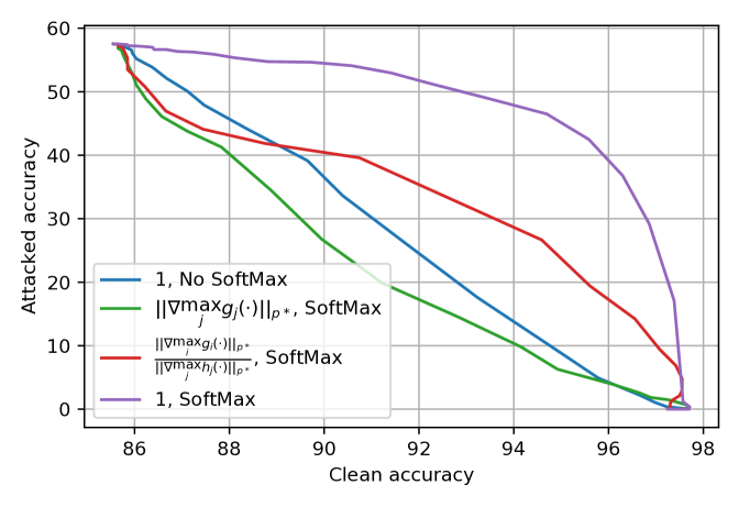
Figure˜1 visualizes the accuracy-robustness trade-off achieved by mixing logits or probabilities with different options. Here, the base classifiers are a pair of standard and adversarially trained ResNet-18s. This “clean accuracy versus PGD10-attacked accuracy” plot concludes that gives the best accuracy-robustness trade-off, and and should be probabilities. Appendix˜A in the supplementary materials confirms this selection by repeating Figure˜1 with alternative model architectures, different robust base classifier training methods, and various attack budgets.
Our selection of differs from used in (Anderson and Sojoudi, 2022b). Intuitively, Anderson and Sojoudi (2022b) used linear classifiers to motivate estimating the base models’ trustworthiness with their gradient magnitudes. When the base classifiers are highly nonlinear neural networks as in our case, while a base classifier’s local Lipschitzness correlates with its robustness, its gradient magnitude is not always a good local Lipschitzness estimator. Additionally, Section˜3.1 offers theoretical intuitions for selecting mixing probabilities over mixing logits.
With these design choices implemented, the formulation Eq.˜3 can be re-parameterized as
| (4) |
where . We take in Eq.˜4, which is a convex combination of base classifier probabilities, as our proposed mixed classifier. Note that Eq.˜4 calculates the mixed classifier logits, acting as a drop-in replacement for existing models which usually produce logits. Removing the logarithm recovers the output probabilities without changing the predicted class.
3.1 Theoretical Certified Robust Radius
In this section, we derive certified robust radii for the mixed classifier introduced in Eq.˜4, given in terms of the robustness properties of and the mixing parameter . The results ensure that despite being more sophisticated than a single model, cannot be easily conquered, even if an adversary attempts to adapt its attack methods to its structure. Such guarantees are of paramount importance for reliable deployment in safety-critical control applications.
Noticing that the base model probabilities satisfy and for all , we introduce the following generalized and tightened notion of certified robustness.
Definition 3.1.
Consider an arbitrary input and let , , and . Then, is said to be certifiably robust at with margin and radius if for all and all such that .
Lemma 3.2.
Let and . If it holds that and is certifiably robust at with margin and radius , then the mixed classifier is robust in the sense that for all such that .
Proof 3.3.
Suppose that is certifiably robust at with margin and radius . Since , it holds that . Let . Consider an arbitrary and such that . Since , it holds that
Thus, it holds that for all , and thus .
Intuitively, Definition 3.1 ensures that all points within a radius from a nominal point have the same prediction as the nominal point, with the difference between the top and runner-up probabilities no smaller than a threshold. For practical classifiers, the robust margin can be straightforwardly estimated by calculating the confidence gap between the predicted and the runner-up classes at an adversarial input obtained with strong attacks.
While most existing provably robust results consider the special case with zero margin, we will show that models built via common methods are also robust with non-zero margins. We specifically consider two types of popular robust classifiers: Lipschitz continuous models (Theorem˜3.5) and RS models (Theorem˜3.7). Here, Lemma 3.2 builds the foundation for proving these two theorems, which amounts to showing that Lipschitz and RS models are robust with non-zero margins and thus the mixed classifiers built with them are robust.
Lemma 3.2 provides further justifications for using probabilities instead of logits in the mixing operation. Intuitively, it holds that is bounded between and , so as long as is relatively large (specifically, at least ), the detrimental effect of ’s probabilities when subject to attack can be bounded and be overcome by . Had we used the logits for , since this quantity cannot be bounded, it would have been much harder to overcome the vulnerability of .
Since we do not make assumptions on the Lipschitzness or robustness of , Lemma 3.2 is tight. To understand this, we suppose that there exists some and such that that make smaller than , indicating that . Since the only information about is that and thus the value can be any number in , it is possible that is smaller than . In this case, it holds that , and thus .
Definition 3.4.
A function is called -Lipschitz continuous if there exists such that for all . The Lipschitz constant of such is defined to be .
Assumption 1
The classifier is robust in the sense that, for all , is -Lipschitz continuous with Lipschitz constant .
Theorem 3.5.
Suppose that Assumption 1 holds, and let be arbitrary. Let . Then, if , it holds that for all such that
| (5) |
Proof 3.6.
Suppose that , and let be such that . Furthermore, let . It holds that
Therefore, is certifiably robust at with margin and radius . Hence, by Lemma 3.2, the claim holds.
We remark that the norm that Theorem˜3.5 certifies may be arbitrary (e.g., , , or ), so long as the Lipschitz constant of the robust network is computed with respect to the same norm.
Assumption 1 is not restrictive in practice. For example, Gaussian RS with smoothing variance yields robust models with -Lipschitz constant (Salman et al., 2019). Moreover, empirically robust methods such as AT and TRADES often train locally Lipschitz continuous models, even though there may not be closed-form theoretical guarantees.
Assumption 1 can be relaxed to the even less restrictive scenario of using local Lipschitz constants over a neighborhood (e.g., a norm ball) around a nominal input (i.e., how flat is near ) as a surrogate for the global Lipschitz constants. In this case, Theorem˜3.5 holds for all within this neighborhood. Specifically, suppose that for an arbitrary input and an attack radius , it holds that and for all and all perturbations such that . Furthermore, suppose that the robust radius , as defined in Eq.˜5 but use the local Lipschitz constant as a surrogate to the global constant , is not smaller than . Then, if the robust base classifier is correct at the nominal point , then the mixed classifier is robust at within the radius . The proof follows that of Theorem˜3.5.
The relaxed Lipschitzness defined above can be estimated for practical differentiable classifiers via an algorithm similar to the PGD attack (Yang et al., 2020). Yang et al. (2020) also showed that many existing empirically robust models, including those trained with AT or TRADES, are in fact locally Lipschitz. Note that Yang et al. (2020) evaluated the local Lipschitz constants of the logits, whereas we analyze the probabilities, whose Lipschitz constants are much smaller. Therefore, Theorem˜3.5 provides important insights into the empirical robustness of the mixed classifier.
An intuitive explanation of Theorem˜3.5 is that if , then , which is the standard Lipschitz-based robust radius of around (see (Fazlyab et al., 2019; Hein and Andriushchenko, 2017) for further discussions on Lipschitz-based robustness). On the other hand, if is too small in comparison to the relative confidence of and put an excess weight into the non-robust classifier , namely, if there exists such that , then , and in this case, we cannot provide non-trivial certified robustness for . If is confident in its prediction, then for all , and therefore this threshold value of becomes , leading to non-trivial certified radii for . However, once we put over of the weight into , a nonzero radius around is no longer certifiable. Since no assumptions on the robustness of around have been made, this is intuitively the best one can expect.
We now move on to tightening the certified radius in the special case when is an RS classifier and our robust radii are defined in terms of the norm.
Assumption 2
The classifier is a (Gaussian) randomized smoothing classifier, i.e., for all , where is a neural model that is non-robust in general. Furthermore, for all , is not 0 almost everywhere or 1 almost everywhere.
Theorem 3.7.
Suppose that Assumption 2 holds, and let be arbitrary. Let and . Then, if , it holds that for all such that
The proof of Theorem˜3.7 is provided in Appendix˜B in the supplementary materials.
To summarize our certified radii, Theorem˜3.5 applies to very general Lipschitz continuous robust base classifiers and arbitrary norms, whereas Theorem˜3.7, applying to the norm and RS base classifiers, strengthens the certified radius by exploiting the stronger Lipschitzness arising from the special structure and smoothness granted by Gaussian convolution operations. Theorems 3.5 and 3.7 guarantee that our proposed robustification cannot be easily circumvented by adaptive attacks.
4 Numerical Experiments
4.1 ’s Influence on Mixed Classifier Robustness
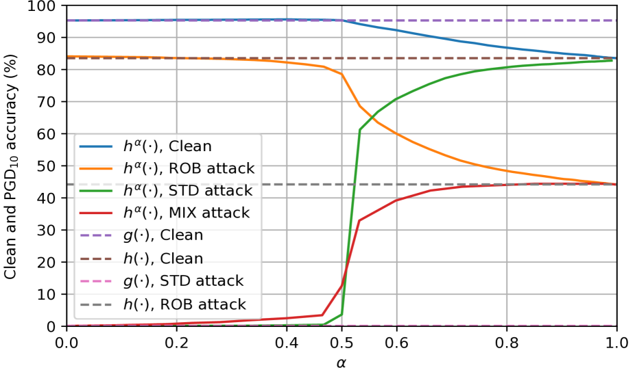
We first use the CIFAR-10 dataset to evaluate the mixed classifier with various values of . We use a ResNet18 model trained on unattacked images as the standard base model and use another ResNet18 trained on PGD20 data as the robust base model . We consider PGD20 attacks that target and individually (abbreviated as STD and ROB attacks and can be regarded as transfer attacks), in addition to the adaptive PGD20 attack generated using the end-to-end gradient of , denoted as the MIX attack.
The test accuracy of each mixed classifier is presented in Figure˜2. As increases, the clean accuracy of converges from the clean accuracy of to the clean accuracy of . In terms of attacked performance, when the attack targets , the attacked accuracy increases with . When the attack targets , the attacked accuracy decreases with , showing that the attack targeting becomes more benign when the mixed classifier emphasizes . When the attack targets the mixed classifier , the attacked accuracy increases with .
When is around , the MIX-attacked accuracy of quickly increases from near zero to more than (two-thirds of ’s attacked accuracy). This observation precisely matches the theoretical intuition from Theorem˜3.5. Meanwhile, when is greater than , the clean accuracy gradually decreases at a much slower rate, leading to the alleviated accuracy-robustness trade-off.
4.2 The Relationship between ’s Robustness and ’s Confidence
This difference in how clean and attacked accuracy change with can be explained by the prediction confidence of the robust base classifier . Specifically, Table˜1 confirms that makes confident correct predictions even when under attack (average robust margin is ). Moreover, ’s robust margin follows a long-tail distribution: the median robust margin is , much larger than the mean. Thus, most attacked inputs correctly classified by are highly confident (i.e., robust with large margins). As Lemma 3.2 suggests, such a property is precisely what the mixed classifier relies on. Intuitively, once becomes greater than and gives more authority over , can use its confidence to correct ’s mistakes under attack.
| Clean Instances | ||
|---|---|---|
| Correct | Incorrect | |
| 0.982 | 0.698 | |
| 0.854 | 0.434 | |
PGD20 Instances Correct Incorrect 0.602 0.998 0.768 0.635
On the other hand, is unconfident when producing incorrect predictions on clean data, with the top two classes’ output probabilities separated by merely . This probability gap again forms a long-tail distribution (the median is which is less than the mean), confirming that rarely makes confident incorrect predictions. Now, consider clean data that correctly classifies and mispredicts. Recall that we assume to be more accurate but less robust, so this scenario should be common. Since is confident (average top two classes probability gap is ) and is usually unconfident, even when and has less authority than in the mixture, can still correct some of the mistakes from .
In summary, is confident when making correct predictions on attacked data while being unconfident when misclassifying clean data, and such a confidence property is the key source of the mixed classifier’s improved accuracy-robustness trade-off. Additional analyses in Appendix˜A with alternative base models imply that multiple existing robust classifiers share this benign confidence property and thus help the mixed classifier improve the trade-off.
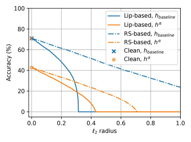
4.3 Visualization of the Certified Robust Radii
Next, we visualize the certified robust radii presented in Theorem˜3.5 and Theorem˜3.7. Since a (Gaussian) RS model with smoothing covariance matrix has an -Lipschitz constant , such a model can be used to simultaneously visualize both theorems, with Theorem˜3.7 giving tighter certificates of robustness. Note that RS models with a larger smoothing variance certify larger radii but achieve lower clean accuracy, and vice versa. Here, we consider the CIFAR-10 dataset and select to be a ConvNeXT-T model with a clean accuracy of , and use the RS models presented in (Zhang et al., 2019) as . For a fair comparison, we select an value such that the clean accuracy of the constructed mixed classifier matches that of another RS model with a smaller smoothing variance. The expectation term in the RS formulation is approximated with the empirical mean of random perturbations drawn from , and the certified radii of are calculated using Theorems 3.5 and 3.7 by setting to . Figure˜3 displays the calculated certified accuracy of and at various attack radii. The ordinate “Accuracy” at a given abscissa “ radius” reflects the percentage of the test data for which the considered model gives a correct prediction as well as a certified radius at least as large as the radius under consideration.
[
: RS with .
: ; is RS with .
][t]
 {subfigure}[
: RS with .
Consider two mixed classifier examples:
: ; is RS with ;
: ; is RS with .
][t]
{subfigure}[
: RS with .
Consider two mixed classifier examples:
: ; is RS with ;
: ; is RS with .
][t]
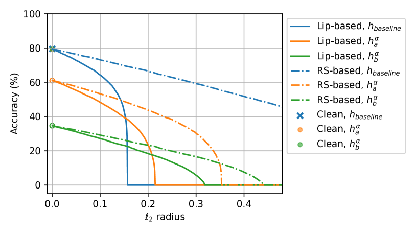
In both subplots of Figure˜3, the certified robustness curves of do not connect to the clean accuracy when . This is because Theorems 3.5 and 3.7 both consider robustness with respect to and do not certify test inputs at which makes incorrect predictions, even though may correctly predict some of these points. This is reasonable because we do not assume any robustness or Lipschitzness of , and is allowed to be arbitrarily incorrect whenever the radius is non-zero.
The Lipschitz-based bound of Theorem˜3.5 allows us to visualize the performance of the mixed classifier when is an -Lipschitz model. In this case, the curves associated with and intersect, with achieving higher certified accuracy at larger radii and certifying more points at smaller radii. Adjusting and the Lipschitz constant of can change the location of this intersection while maintaining the clean accuracy. Thus, the mixed classifier allows for optimizing the certified accuracy at a particular radius without sacrificing clean accuracy.
The RS-based bound from Theorem˜3.7 captures the behavior of the mixed classifier when is an RS model. For both and , the RS-based bounds certify larger radii than the corresponding Lipschitz-based bounds. Nonetheless, can certify more points with the RS-based guarantee. Intuitively, this phenomenon suggests that RS models can yield correct but low-confidence predictions when under large-radius attack, and thus may not be best-suited for our mixing operation, which relies on robustness with non-zero margins. Meanwhile, Lipschitz models, a more general and common class of models, exploit the mixing operation more effectively. Moreover, as shown in Figure˜2 and Table˜1, empirically robust models often yield high-confidence correct predictions when under attack, making them more suitable to be used as ’s robust base classifier.
5 Conclusions
This work proposes to mix the predicted probabilities of an accurate classifier and a robust classifier to mitigate the accuracy-robustness trade-off. These two base classifiers can be pre-trained, and the resulting mixed classifier requires no additional training. Theoretical results certify that the mixed classifier inherits the robustness of the robust base model under realistic assumptions. Empirical evaluations show that our method approaches the high accuracy of the latest standard models while retaining the robustness of modern robust classification methods. Hence, this work provides a foundation for future research to focus on either accuracy or robustness without sacrificing the other, providing additional incentives for deploying robust models in safety-critical control.
This work was supported by grants from ONR, NSF, and C3 AI.
References
- Alam et al. (2022) Manaar Alam, Shubhajit Datta, Debdeep Mukhopadhyay, Arijit Mondal, and Partha Pratim Chakrabarti. Resisting adversarial attacks in deep neural networks using diverse decision boundaries. arXiv preprint arXiv:2208.08697, 2022.
- Anderson et al. (2020) Brendon Anderson, Ziye Ma, Jingqi Li, and Somayeh Sojoudi. Tightened convex relaxations for neural network robustness certification. In IEEE Conference on Decision and Control, 2020.
- Anderson and Sojoudi (2022a) Brendon G Anderson and Somayeh Sojoudi. Data-driven certification of neural networks with random input noise. IEEE Transactions on Control of Network Systems, 2022a.
- Anderson and Sojoudi (2022b) Brendon G. Anderson and Somayeh Sojoudi. Certified robustness via locally biased randomized smoothing. In Learning for Dynamics and Control Conference, 2022b.
- Bai et al. (2022a) Yatong Bai, Tanmay Gautam, Yu Gai, and Somayeh Sojoudi. Practical convex formulation of robust one-hidden-layer neural network training. American Control Conference, 2022a.
- Bai et al. (2022b) Yatong Bai, Tanmay Gautam, and Somayeh Sojoudi. Efficient global optimization of two-layer ReLU networks: Quadratic-time algorithms and adversarial training. SIAM Journal on Mathematics of Data Science, 2022b.
- Balaji et al. (2019) Yogesh Balaji, Tom Goldstein, and Judy Hoffman. Instance adaptive adversarial training: Improved accuracy tradeoffs in neural nets. arXiv preprint arXiv:1910.08051, 2019.
- Bojarski et al. (2016) Mariusz Bojarski, Davide Del Testa, Daniel Dworakowski, Bernhard Firner, Beat Flepp, Prasoon Goyal, Lawrence D. Jackel, Mathew Monfort, Urs Muller, Jiakai Zhang, et al. End to end learning for self-driving cars. arXiv preprint arXiv:1604.07316, 2016.
- Chen et al. (2020) Tianlong Chen, Sijia Liu, Shiyu Chang, Yu Cheng, Lisa Amini, and Zhangyang Wang. Adversarial robustness: From self-supervised pre-training to fine-tuning. In IEEE Conference on Computer Vision and Pattern Recognition, 2020.
- Cohen et al. (2019) Jeremy Cohen, Elan Rosenfeld, and Zico Kolter. Certified adversarial robustness via randomized smoothing. In International Conference on Machine Learning, 2019.
- Eykholt et al. (2018) Kevin Eykholt, Ivan Evtimov, Earlence Fernandes, Bo Li, Amir Rahmati, Chaowei Xiao, Atul Prakash, Tadayoshi Kohno, and Dawn Song. Robust physical-world attacks on deep learning visual classification. In IEEE Conference on Computer Vision and Pattern Recognition, 2018.
- Fan et al. (2021) Lijie Fan, Sijia Liu, Pin-Yu Chen, Gaoyuan Zhang, and Chuang Gan. When does contrastive learning preserve adversarial robustness from pretraining to finetuning? In Advances in Neural Information Processing Systems, 2021.
- Fazlyab et al. (2019) Mahyar Fazlyab, Alexander Robey, Hamed Hassani, Manfred Morari, and George Pappas. Efficient and accurate estimation of Lipschitz constants for deep neural networks. In Advances in Neural Information Processing Systems, 2019.
- Goodfellow et al. (2015) Ian J. Goodfellow, Jonathon Shlens, and Christian Szegedy. Explaining and harnessing adversarial examples. In International Conference on Learning Representations, 2015.
- Gowal et al. (2021) Sven Gowal, Sylvestre-Alvise Rebuffi, Olivia Wiles, Florian Stimberg, Dan A. Calian, and Timothy Mann. Improving robustness using generated data. arXiv preprint arXiv:2110.09468, 2021.
- Hein and Andriushchenko (2017) Matthias Hein and Maksym Andriushchenko. Formal guarantees on the robustness of a classifier against adversarial manipulation. In Advances in Neural Information Processing Systems, 2017.
- Hu et al. (2020) Ting-Kuei Hu, Tianlong Chen, Haotao Wang, and Zhangyang Wang. Triple wins: Boosting accuracy, robustness and efficiency together by enabling input-adaptive inference. In International Conference on Learning Representations, 2020.
- Huang et al. (2017) Sandy H. Huang, Nicolas Papernot, Ian J. Goodfellow, Yan Duan, and Pieter Abbeel. Adversarial attacks on neural network policies. In International Conference on Learning Representations, 2017.
- Jia et al. (2022) Xiaojun Jia, Yong Zhang, Baoyuan Wu, Ke Ma, Jue Wang, and Xiaochun Cao. LAS-AT: Adversarial training with learnable attack strategy. In IEEE Conference on Computer Vision and Pattern Recognition, 2022.
- Krizhevsky (2012) Alex Krizhevsky. Learning multiple layers of features from tiny images, 2012. URL https://www.cs.toronto.edu/˜kriz/learning-features-2009-TR.pdf.
- Kumar et al. (2022) Aounon Kumar, Alexander Levine, and Soheil Feizi. Policy smoothing for provably robust reinforcement learning. In International Conference on Learning Representations, 2022.
- Kurakin et al. (2017) Alexey Kurakin, Ian J. Goodfellow, and Samy Bengio. Adversarial machine learning at scale. In International Conference on Learning Representations, 2017.
- Lamb et al. (2019) Alex Lamb, Vikas Verma, Juho Kannala, and Yoshua Bengio. Interpolated adversarial training: Achieving robust neural networks without sacrificing too much accuracy. In ACM Workshop on Artificial Intelligence and Security, 2019.
- Levine et al. (2019) Alexander Levine, Sahil Singla, and Soheil Feizi. Certifiably robust interpretation in deep learning. arXiv preprint arXiv:1905.12105, 2019.
- Levine et al. (2016) Sergey Levine, Chelsea Finn, Trevor Darrell, and Pieter Abbeel. End-to-end training of deep visuomotor policies. The Journal of Machine Learning Research, 17(1):1334–1373, 2016.
- Li et al. (2019) Bai Li, Changyou Chen, Wenlin Wang, and Lawrence Carin. Certified adversarial robustness with additive noise. In Advances in Neural Information Processing Systems, 2019.
- Liu et al. (2019) Aishan Liu, Xianglong Liu, Jiaxin Fan, Yuqing Ma, Anlan Zhang, Huiyuan Xie, and Dacheng Tao. Perceptual-sensitive GAN for generating adversarial patches. In The AAAI Conference on Artificial Intelligence, 2019.
- Liu et al. (2018) Xuanqing Liu, Minhao Cheng, Huan Zhang, and Cho-Jui Hsieh. Towards robust neural networks via random self-ensemble. In European Conference on Computer Vision, 2018.
- Liu et al. (2022) Zhuang Liu, Hanzi Mao, Chao-Yuan Wu, Christoph Feichtenhofer, Trevor Darrell, and Saining Xie. A ConvNet for the 2020s. In IEEE Conference on Computer Vision and Pattern Recognition, 2022.
- Ma and Sojoudi (2021) Ziye Ma and Somayeh Sojoudi. A sequential framework towards an exact SDP verification of neural networks. In International Conference on Data Science and Advanced Analytics, 2021.
- Madry et al. (2018) Aleksander Madry, Aleksandar Makelov, Ludwig Schmidt, Dimitris Tsipras, and Adrian Vladu. Towards deep learning models resistant to adversarial attacks. In International Conference on Learning Representations, 2018.
- Nguyen et al. (2015) Anh Nguyen, Jason Yosinski, and Jeff Clune. Deep neural networks are easily fooled: High confidence predictions for unrecognizable images. In IEEE Conference on Computer Vision and Pattern Recognition, 2015.
- Pang et al. (2019) Tianyu Pang, Kun Xu, Chao Du, Ning Chen, and Jun Zhu. Improving adversarial robustness via promoting ensemble diversity. In International Conference on Machine Learning, 2019.
- Pang et al. (2022) Tianyu Pang, Min Lin, Xiao Yang, Jun Zhu, and Shuicheng Yan. Robustness and accuracy could be reconcilable by (proper) definition. arXiv preprint arXiv:2202.10103, 2022.
- Pfrommer et al. (2023) Samuel Pfrommer, Brendon G Anderson, and Somayeh Sojoudi. Projected randomized smoothing for certified adversarial robustness. Transactions on Machine Learning Research, 2023.
- Raghunathan et al. (2020) Aditi Raghunathan, Sang Michael Xie, Fanny Yang, John C. Duchi, and Percy Liang. Understanding and mitigating the tradeoff between robustness and accuracy. In International Conference on Machine Learning, 2020.
- Rebuffi et al. (2021) Sylvestre-Alvise Rebuffi, Sven Gowal, Dan A Calian, Florian Stimberg, Olivia Wiles, and Timothy Mann. Fixing data augmentation to improve adversarial robustness. arXiv preprint arXiv:2103.01946, 2021.
- Salman et al. (2019) Hadi Salman, Jerry Li, Ilya Razenshteyn, Pengchuan Zhang, Huan Zhang, Sebastien Bubeck, and Greg Yang. Provably robust deep learning via adversarially trained smoothed classifiers. Advances in Neural Information Processing Systems, 2019.
- Schmidt et al. (2018) Ludwig Schmidt, Shibani Santurkar, Dimitris Tsipras, Kunal Talwar, and Aleksander Madry. Adversarially robust generalization requires more data. Advances in Neural Information Processing Systems, 31, 2018.
- Sehwag et al. (2022) Vikash Sehwag, Saeed Mahloujifar, Tinashe Handina, Sihui Dai, Chong Xiang, Mung Chiang, and Prateek Mittal. Robust learning meets generative models: Can proxy distributions improve adversarial robustness? In International Conference on Learning Representations, 2022.
- Shafahi et al. (2019) Ali Shafahi, Mahyar Najibi, Mohammad Amin Ghiasi, Zheng Xu, John Dickerson, Christoph Studer, Larry S Davis, Gavin Taylor, and Tom Goldstein. Adversarial training for free! Advances in Neural Information Processing Systems, 2019.
- Sutton and Barto (2018) Richard S. Sutton and Andrew G. Barto. Reinforcement Learning: An Introduction. MIT press, 2018.
- Szegedy et al. (2014) Christian Szegedy, Wojciech Zaremba, Ilya Sutskever, Joan Bruna, Dumitru Erhan, Ian Goodfellow, and Rob Fergus. Intriguing properties of neural networks. In International Conference on Learning Representations, 2014.
- Tramèr et al. (2018) Florian Tramèr, Alexey Kurakin, Nicolas Papernot, Ian J. Goodfellow, Dan Boneh, and Patrick D. McDaniel. Ensemble adversarial training: Attacks and defenses. In International Conference on Learning Representations, 2018.
- Tramèr et al. (2020) Florian Tramèr, Nicholas Carlini, Wieland Brendel, and Aleksander Madry. On adaptive attacks to adversarial example defenses. In Advances in Neural Information Processing Systems, 2020.
- Tsipras et al. (2019) Dimitris Tsipras, Shibani Santurkar, Logan Engstrom, Alexander Turner, and Aleksander Madry. Robustness may be at odds with accuracy. In International Conference on Learning Representations, 2019.
- Wu et al. (2017) Bichen Wu, Forrest Iandola, Peter H. Jin, and Kurt Keutzer. SqueezeDet: Unified, small, low power fully convolutional neural networks for real-time object detection for autonomous driving. In IEEE Conference on Computer Vision and Pattern Recognition Workshops, 2017.
- Wu et al. (2022) Fan Wu, Linyi Li, Zijian Huang, Yevgeniy Vorobeychik, Ding Zhao, and Bo Li. CROP: Certifying robust policies for reinforcement learning through functional smoothing. In International Conference on Learning Representations, 2022.
- Yang et al. (2020) Yao-Yuan Yang, Cyrus Rashtchian, Hongyang Zhang, Russ R. Salakhutdinov, and Kamalika Chaudhuri. A closer look at accuracy vs. robustness. In Annual Conference on Neural Information Processing Systems, 2020.
- Zhang and Wang (2019) Haichao Zhang and Jianyu Wang. Defense against adversarial attacks using feature scattering-based adversarial training. In Annual Conference on Neural Information Processing Systems, 2019.
- Zhang et al. (2019) Hongyang Zhang, Yaodong Yu, Jiantao Jiao, Eric P. Xing, Laurent El Ghaoui, and Michael I. Jordan. Theoretically principled trade-off between robustness and accuracy. In International Conference on Machine Learning, 2019.
- Zheng et al. (2020) Haizhong Zheng, Ziqi Zhang, Juncheng Gu, Honglak Lee, and Atul Prakash. Efficient adversarial training with transferable adversarial examples. In IEEE Conference on Computer Vision and Pattern Recognition, 2020.
- Zheng et al. (2021) Yaowei Zheng, Richong Zhang, and Yongyi Mao. Regularizing neural networks via adversarial model perturbation. In IEEE Conference on Computer Vision and Pattern Recognition, 2021.
Appendix A Additional Empirical Support for
[ConvNeXT-T and TRADES WRN-34 under PGD attack.][t]
 {subfigure}[Standard and AT ResNet18s under PGD attack.][t]
| Attack Budget; PGD Steps | Architecture | Architecture | |
|---|---|---|---|
| Figure˜1 | , , 10 Steps | Standard ResNet18 | -adversarially-trained ResNet18 |
| Figure˜4 | , , 20 Steps | Standard ConvNeXT-T | TRADES WideResNet-34 |
| Figure˜4 | , , 20 Steps | Standard ResNet18 | -adversarially-trained ResNet18 |
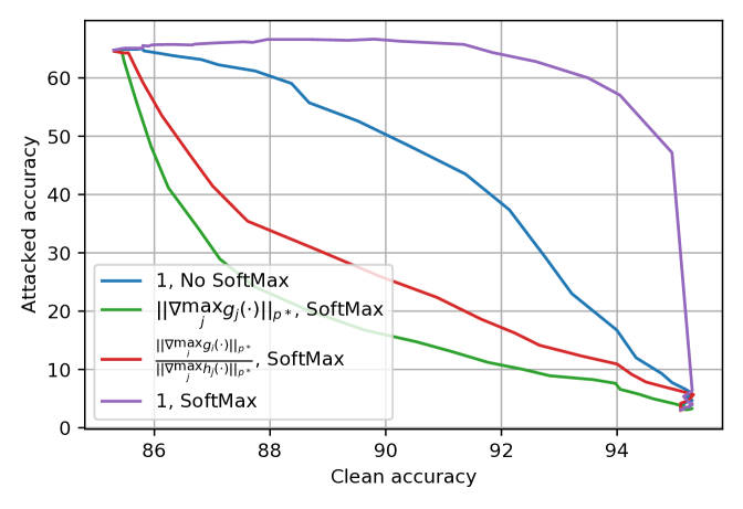
Finally, we use additional empirical evidence (Figures 4 and 4) to show that is the appropriate choice for the mixed classifier and that the probabilities should be used for the mixture. While most experiments in this paper are based on the popular ResNet architecture, our method does not depend on any ResNet properties. Therefore, for the experiment in Figure˜4, we select a more modern ConvNeXT-T model (Liu et al., 2022) pre-trained on ImageNet-1k as an alternative architecture for . We also use a robust model trained via TRADES in place of an adversarially-trained network for for the interest of diversity. Additionally, although most of our experiments are based on attacks, the proposed method applies to all attack budgets. In Figure˜4, we provide an example that considers the attack. The experiment settings are summarized in Table˜2.
Figures 4 and 4 confirm that setting to the constant achieves the best trade-off curve between clean and attacked accuracy, and that mixing the probabilities outperforms mixing the logits. This result aligns with the conclusions of Figure˜1 and our theoretical analyses.
For all three cases listed in Table˜2, the mixed classifier reduces the error rate of on clean data by half while maintaining of ’s attacked accuracy. This observation suggests that the mixed classifier noticeably alleviates the accuracy-robustness trade-off. Additionally, our method is especially suitable for applications where the clean accuracy gap between and is large. On easier datasets such as MNIST and CIFAR-10, this gap has been greatly reduced by the latest advancements in constructing robust classifiers. However, on harder tasks such as CIFAR-100 and ImageNet-1k, this gap is still large, even for state-of-the-art methods. For these applications, standard classifiers often benefit much more from pre-training on larger datasets than robust models.
Appendix B Proof of Theorem˜3.7
Theorem B.5 (Restated).
Suppose that Assumption 2 holds, and let be arbitrary. Let and . Then, if , it holds that for all such that
Proof B.6.
First, note that since every is not 0 almost everywhere or 1 almost everywhere, it holds that for all and all . Now, suppose that , and let be such that . Let . Define the function by
Furthermore, define by .
Then, since and for all , it must be the case that for all and all , and hence, for all , the function is -Lipschitz continuous with Lipschitz constant (see (Levine et al., 2019, Lemma 1), or Lemma 2 in (Salman et al., 2019) and the discussion thereafter). Therefore,
| (6) |
for all . Applying Eq.˜6 for yields that
| (7) |
Since monotonically increases and for all , applying Eq.˜6 to gives
| (8) |
Subtracting Eq.˜8 from Eq.˜7 gives that
for all . By the definitions of , , and , the right-hand side of this inequality equals zero. Since monotonically increases, we find that for all . Thus,
Hence, for all , so is certifiably robust at with margin and radius . Therefore, by Lemma 3.2, it holds that for all such that , which concludes the proof.