Mock galaxy redshift catalogues from simulations: implications for Pan-STARRS1
Abstract
We describe a method for constructing mock galaxy catalogues which are well suited for use in conjunction with large photometric surveys. We use the semi-analytic galaxy formation model of Bower et al. implemented in the Millennium N-body simulation of the evolution of dark matter clustering in a CDM cosmology. We apply our method to the specific case of the surveys soon to commence with PS1, the first of 4 telescopes planned for the Pan-STARRS system. PS1 has 5 photometric bands, and and will carry out an all-sky “3” survey and a medium deep survey (MDS) over 84 sq. deg. We calculate the expected magnitude limits for extended sources in the two surveys. We find that, after 3 years, the 3 survey will have detected over galaxies in all 5 bands, 10 million of which will lie at redshift , while the MDS will have detected over galaxies with 0.5 million lying at . These numbers at least double if detection in the shallowest band, is not required. We then evaluate the accuracy of photometric redshifts estimated using an off-the-shelf photo- code. With the bands alone it is possible to achieve an accuracy in the 3 survey of in the range , which could be reduced by about 15% using near infrared photometry from the UKIDDS survey, but would increase by about 25% for the deeper sample without the band photometry. For the MDS an accuracy of is achievable for using . A dramatic improvement in accuracy is possible by selecting only red galaxies. In this case, is achievable for 100 million galaxies at in the 3 survey and for 30 million galaxies in the MDS at . We investigate the effect of using photometric redshifts in the estimate of the baryonic acoustic oscillation scale. We find that PS1 will achieve a similar accuracy in this estimate as a spectroscopic survey of 20 million galaxies.
keywords:
cosmology: large-scale structure of the Universe – cosmology: cosmological parameters1 Introduction
Studies of the cosmic large structure were brought to a new level by the two large galaxy surveys of the past decade, the “2-degree-field galaxy redshift survey (2dFGRS; Colless et al., 2001) and the Sloan Digital Sky Survey (SDSS York et al., 2000). The former relied on photographic plates for its source catalogue while the latter was compiled from the largest CCD based photometric survey to date. Most of the large-scale structure studies carried out with these surveys made use of spectroscopic redshifts, for about 220,000 galaxies in the case of the 2dFGRS and 585,719 galaxies in the case of the SDSS (Strauss et al., 2002). These surveys achieved important advances such as the confirmation of the existence of dark energy (Efstathiou et al., 2002; Tegmark et al., 2004) and the discovery of baryonic acoustic oscillations (Percival et al., 2001; Cole et al., 2005; Eisenstein et al., 2005). Yet, a number of fundamental questions on the cosmic large-scale structure remain unanswered, such as the identity of the dark matter and the nature of the dark energy.
Further progress in the subject is likely to require a new generation of galaxy surveys at least one order of magnitude larger than the 2dFGRS and the SDSS. Unfortunately, measuring redshifts for millions of galaxies is infeasible with current instrumentation. Attention has therefore shifted to the possibility of carrying out extremely large surveys of galaxies in which, instead of using spectroscopy, redshifts are estimated from deep multi-band photometry. Although the accuracy of these estimates is limited, this strategy can yield measurements for hundreds of millions of galaxies or more. Several instruments are currently being planned to carry out such a programme. The most advanced is the Panoramic Survey Telescope & Rapid Response System (Chambers, 2006). Of an eventual 4 telescopes for this system, the first one, PS1, is now in its final commissioning stages and is expected to begin surveying the sky early in 2009. This telescope is likely to be quickly followed by the full Pan-STARRS system and by the Large Synoptic Survey Telescope (LSST Tyson, 2002). Several other smaller photometric surveys are currently underway (UKIDSS, Megacam etc. Lawrence et al., 2007; Boulade et al., 2003).
One of the important lessons learned from previous surveys, including 2dFGRS and SDSS, is the paramount importance of careful modelling of the survey data for the extraction of robust astrophysical results. Such modelling is best achieved using large cosmological simulations to follow the growth of structure in a specified cosmological background. The simulations can be used to create mock versions of the real survey in which the geometry and selection effects are reproduced. Such mock surveys allow a rigorous assessment of statistical and systematic errors, aid in the design of new statistical analyses and enable the survey results to be directly related to cosmological theory. Mock catalogues based on cosmological simulations were first used in the 1980s, in connection with the CfA galaxy survey (Davis et al., 1985; White et al., 1988) and redshift surveys of IRAS galaxies (Saunders et al., 1991) and have been extensively deployed for analyses of the 2dFGRS and the SDSS (Cole et al., 1998; Blaizot et al., 2006).
The recent determination of the values of the cosmological parameters by a combination of microwave background and large-scale structure data (e.g. Sánchez et al., 2006; Komatsu et al., 2008) has removed one major layer of uncertainty in the execution of cosmological simulations. N-body techniques are now sufficiently sophisticated that the evolution of the dark matter can be followed with impressive precision from the epoch of recombination to the present (Springel et al., 2005). The main uncertainty lies in calculating the evolution of the baryonic component of the Universe.
The size of the planned photometric surveys and the need to understand and quantify uncertainties in estimates of photometric redshifts and their consequences for diagnostics of large-scale structure pose novel challenges for the construction of mock surveys. The simulations need to be large enough to emulate the huge volumes that will be surveyed and, at the same time, the modelling of the galaxy population needs to be sufficiently realistic to allow an assessment of the uncertainties introduced by photometric redshifts. At present, the only technique that can satisfy both these two requirements is the combination of large N-body simulations with semi-analytic modelling of galaxy formation.
Semi-analytic models of galaxy formation are able to follow the evolution of the baryonic component in a cosmological volume by making a number of simplifying assumptions, most notably that gas cooling into halos can be calculated in a spherically symmetric approximation (White & Frenk, 1991). Once the gas has cooled, these models employ simple physically based rules, akin to those used in hydrodynamic simulations, to model star formation and evolution and a variety of feedback processes. The analytical nature of these models makes it possible to investigate galaxy formation in large volumes and to include, in a controlled fashion, a variety of processes, such as dust absorption and emission, that are currently beyond the reach of hydrodynamic simulations. (For a review of this approach, see Baugh, 2006). It is reassuring that the simplified treatment of gas cooling in these models agrees remarkably well with the results of full hydrodynamic simulations (Helly et al., 2003; Yoshida et al., 2002).
An important feature of semi-analytic models is that they are able to reproduce the local galaxy luminosity function from first principles (e.g. Cole et al., 2000; Benson et al., 2003; Hatton et al., 2003; Baugh et al., 2005; Kang et al., 2005, 2006; Bower et al., 2006; Croton et al., 2006; De Lucia et al., 2006) and, in the most recent models, also its evolution to high redshift (Bower et al., 2006; De Lucia et al., 2006; Lacey et al., 2008). These recent models also provide a good match to the distribution of galaxy colours, which is particularly relevant for problems relating to photometric redshifts. And, of course, the models also calculate many properties which are not directly observable (e.g. rest-frame fluxes, stellar masses, etc) but which are important for the interpretation of the data.
There are currently two main approaches to the estimation of photometric redshifts. One employs an empirical relation, obtained by fitting a polynomial or a more general function derived by an artificial neural network, between redshift and observed properties, such as fluxes in specified passbands (e.g. Connolly et al., 1995; Brunner et al., 2000; Sowards-Emmerd et al., 2000; Firth et al., 2003; Collister & Lahav, 2004). The second method is based on fitting the observed spectral energy distribution (SED) with a set of galaxy templates (e.g. Sawicki et al., 1997; Giallongo et al., 1998; Bolzonella et al., 2000; Benítez, 2000; Bender et al., 2001; Csabai et al., 2003), obtained either from observations of the local universe (e.g. Coleman et al., 1980) or from synthetic spectra (e.g. Bruzual & Charlot, 1993, 2003). Some authors (e.g. Collister & Lahav, 2004) claim that the empirical fitting method can give smaller redshift errors, but this method relies on having a well-matched spectroscopic subsample that reaches the same depth in every band as the photometric survey. Unfortunately, for Pan-STARRS or LSST this is going to be challenging and to be conservative in this initial investigation we use Hyper- because it does not require a training set.
In this paper, we describe a method for generating mock catalogues suitable, in principle, for the next generation of large photometric surveys. As an example, we construct mocks surveys tailored to PS1. PS1 will carry out two, 3-year long surveys in 5 bands (), the “ survey” which will cover three quarters of the sky to a depth of about and the “medium deep survey” (MDS) which will cover sq deg to a point sources depth of (AB system). The former will enable a comprehensive list of large-scale structure measurements, including the integrated Sachs-Wolfe effect and baryonic acoustic oscillations. The latter will be used to study clustering on small and intermediate scales, as well as galaxy evolution. To construct the mocks we use the semi-analytic model of Bower et al. (2006, hereafter B06) as implemented in the Millennium simulation (Springel et al., 2005). A sophisticated adaptive template method based on the work of Bender et al. (2001) will be employed for the genuine PS1 survey. The method has been applied in the photo- measurements of FORS Deep Field galaxies (Gabasch et al., 2004) and achieved with only outliers. However, the method requires precise calibration of zeropoints in all filters using the colour-colour plots of stars, and a control sample of spectroscopic redshifts. Consequently this method cannot be rigorously tested until genuine PS1 data is available. Therefore, for a first look at the photo- performance of PS1, we adopt the standard SED fitting method as implemented in the Hyper- for our mock catalogues.
The paper is organised as follows. In §2, we briefly summarise the models and detail the process of constructing mock galaxy catalogues. In §3 we analyse some of their properties and in §4 we use the mock catalogues to assess the accuracy with with photometric redshifts will be estimated by PS1. In §5, we discuss how these uncertainties are likely to affect the accuracy with which baryonic acoustic oscillations, one the main targets for PS1, can be measured in the survey. Finally, in §6, we discuss our results and present our conclusions.
2 Mock catalogue construction
In this section we describe how we construct mock catalogues. In §2.1 we describe the semi-analytic galaxy formation code that we use. In §2.2 we compare the luminosities and sizes of the model galaxies to SDSS data and modify them to improve the accuracy of the mocks. Finally in §2.3 we describe how the mock catalogues themselves are built.
2.1 The galaxy formation model
The first step in the process of generating a mock catalogue is to produce a population of model galaxies over the required redshift range. We use the galform semi-analytic model of galaxy formation (Cole et al., 2000; Benson et al., 2003; Baugh et al., 2005; Bower et al., 2006) to do this. galform calculates the key processes involved in galaxy formation: (i) the growth of dark matter halos by accretion and mergers; (ii) radiative cooling of gas within halos; (iii) star formation and associated feedback processes due to supernova explosions and stellar winds; (iv) the suppression of gas cooling in halos with quasistatic hot atmospheres and accretion driven feedback from supermassive black holes (see Malbon et al. (2007) for a description of the model of black hole growth); (v) galaxy mergers and the associated bursts of star formation; (vi) the chemical evolution of the hot and cold gas, and the stars.
galform uses physically motivated recipes to model these processes. Due to the complex nature of many of them, the model necessarily contains parameters which are set by requiring that it should reproduce a subset of properties of the observed galaxy population (see Cole et al., 2000; Baugh, 2006, for a discussion of the philosophy behind setting the values of the model parameters).
galform predicts star formation histories for the population of galaxies at any specified redshift. These histories are far more complicated than the simple, exponentially decaying star formation laws sometimes assumed in the literature (for examples of star formation histories of galform galaxies, see Baugh, 2006). The galform histories have the advantage that they are produced using an astrophysical model in which the supply of gas available for star formation is set by source and sink processes. The sources are the infall of new material due to gas cooling and galaxy mergers and gas recycling from previous generations of stars. The sinks are star formation and the reheating or removal of cooled gas by feedback processes. The metallicity of the gas consumed in star formation is modelled using the instantaneous recycling approximation and by following the transfer of metals between the hot and cold gas, and the stellar reservoirs (see Fig. 3 of Cole et al., 2000).
The model outputs the broad band magnitudes of each galaxy for a set of specified filters. In this paper we use the PS1 filter set (, , , , ) (Chambers, 2006), augmented by a few additional filters where some of the PS1 galaxies may be observed as part of other observational programmes (, , , , ). In addition to the magnitudes of model galaxies in the observer’s frame, we also output the rest frame colour, in order to distinguish between red and blue galaxy populations. galform tracks the bulge and disk components of the galaxies separately (Baugh et al., 1996). The scale sizes of the disk and bulge (assumed to follow an exponential profile and an -law in projection, respectively) are also calculated (Cole et al., 2000) (see Almeida et al., 2007, for a test of the prescription for computing the size of the spheroid component).
The B06 model which we use in this paper employs halo merger trees extracted from the Millennium N-body simulation of a -cold dark matter universe (Springel et al., 2005). The model gives a very good reproduction of the shape of the present day galaxy luminosity function in the optical and near-infrared. Also of particular relevance for the predictions presented here is the fact that this model matches the observed evolution of the galaxy luminosity function.
2.2 Improving the match to SDSS observations
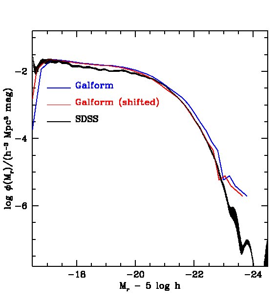
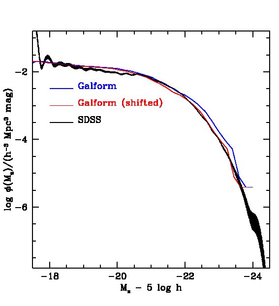
To make the mocks as realistic as possible, we modify the luminosities and sizes of the model galaxies to give a better fit to SDSS data. Although both the -band and K-band luminosity functions of the B06 model have been shown to agree well with observations of the local universe, the agreement is not perfect and a shift of magnitude faintwards in all bands improves the match to the data as can be seen in Fig. 1. The original B06 K-band luminosity functions also match observations up to redshift (Bower et al., 2006), although the observational error bars are relatively large. Hence, even after applying the 0.15 magnitude shift the agreement between model and high redshift observations remains reasonably good.
The galform magnitudes we have been dealing with so far are total integrated magnitudes. In reality all but the most distant galaxies in the survey will be resolved over several pixels and will have lower signal to noise in each of these pixels than a point source would. To take this into account it proves convenient to use Petrosian (1976) magnitudes. These have the advantage over fixed aperture magnitudes that, for a given luminosity profile shape, they measure a fixed fraction of the total luminosity independently of the angular size and surface brightness of the galaxy. The Petrosian flux within times the Petrosian radius, , is:
| (1) |
where is the surface brightness profile of the galaxy. The Petrosian radius is defined such that at this radius, the ratio of the local surface brightness in an annulus at to the mean surface brightness within , is equal to some constant value , specifically:
| (2) |
We choose the parameter values as and as adopted in the SDSS (e.g. Yasuda et al., 2001).
We decompose the surface brightness profile of each galaxy, , into the superposition of a disk and a bulge: . The disk component is taken to have a pure exponential profile:
| (3) |
and the bulge a pure de Vaucouleurs profile :
| (4) |
Given these assumptions, and assuming the disks are face-on, we can compute the Petrosian radius by solving Eqn. (2) for each galform galaxy.
While galform does provide an estimate of the disk and bulge sizes, it has been shown by Almeida et al. (2007) that the early type galaxy sizes of the B06 model are not in particularly good agreement with the SDSS observational results. Therefore, for the purposes of producing more realistic mocks, we modify the galaxy sizes so as to match the SDSS results given by Shen et al. (2003).
To do this we need to separate the galaxies into early and late types and apply separate corrections to each population. First, we use the concentration parameter defined as to separate our galaxies into early and late types, where and are the Petrosian and light radii respectively. We then calculate the ratio of the galform galaxy size to the mean found by Shen et al. (2003) for SDSS galaxies as a function of galaxy magnitude and obtain the average correction factor as a function of magnitude required for the galform galaxies to match the SDSS size data. For early type galaxies at redshift Shen et al. (2003) parameterised the relation between Petrosian half-light radii in the -band, , and absolute -band magnitude, , as
| (5) |
with and . While for late type galaxies they found
| (6) |
with , , and . To correct the galform galaxy sizes at other redshifts we adopt for late type galaxies and for early type galaxies. The former is the relation given by Bouwens & Silk (2002) which agrees with a combination of SDSS, GEMS and FIRES survey data (Trujillo et al., 2006). The relation for early type galaxies is obtained by taking a linear fit to the data given by Trujillo et al. (2006). Finally, we apply a linear relation between and the Petrosian radius, .
2.3 Building the mock catalogues
Our goal here is to generate mock catalogues which have the distribution of galaxy redshifts and magnitudes expected for the various PS1 catalogues. For the purposes of this paper, we do not need to retain the clustering information contained in the Millennium Simulation. We are effectively generating a Monte-Carlo realisation of the redshift distribution expected for a given set of magnitude limits. The production of mock catalogues with clustering information will be described in a later paper.
There are 37 discrete output epochs in the Millennium simulation between and . The spacing of the output times is comparable to the typical error on the estimated value of photometric redshifts, as we will see later. To avoid the introduction of systematic errors caused by the discrete spacing of simulation output times, previous work to build mock catalogues used an interpolation of galaxy properties between output times (Blaizot et al., 2005). We follow an alternative approach in this paper. We have generated nine additional outputs which are evenly spaced between each pair of Millennium simulation outputs. To produce galform output at each of these intermediate steps, the Millennium simulation merger trees ending at the nearest simulation output are used but their redshifts are re-labelled to match the required redshift. Then galform computes the star formation history up to the new output redshift, following the baryonic physics up to that point. This results in a much finer spacing of effective output redshifts which fully takes account of k-corrections, star formation and stellar evolution, but ignores the evolution in the dark matter distribution between the chosen output redshift and the nearest simulation redshift.
To generate a mock catalogue with a smooth redshift distribution we proceed as follows. At each of our closely spaced grid of redshifts, , we have a galform output dataset consisting of a set of galform galaxies sampling a fixed comoving volume down to a sufficiently deep absolute magnitude. To each of these datasets we apply a magnitude limit and record the number of galaxies, , that remain. The comoving number density of galaxies expected brighter than the limit is then and the number we expect per unit redshift in the survey is , where is the solid angle of the survey and is the comoving volume per unit redshift and solid angle for the adopted cosmology. This can be used to compute, , the number of galaxies expected in the survey in a redshift bin , centred at a given redshift, . To create a continuous redshift distribution we sample at random this number of galaxies from the corresponding galform output and assign them a random redshift in the interval such that we uniformly sample the volume redshift relation. As we have perturbed the redshift of each galaxy, we correspondingly perturb its apparent magnitude according to the difference in distance modulus between the output and assigned redshift. We will see that the residual redshift quantisation in the evolutionary and k-corrections is small compared with the precision achievable for the photometric redshifts. Therefore these residual discreteness effects are not important in the photometric redshift error estimation.
For the purpose of producing predictions for the redshift distribution and number counts of galaxies in PS1 surveys, and to provide an input catalogue with which to test photometric redshift estimators, we generate a mock catalogue which corresponds to a solid angle of 10 square degrees. We generate predictions for the survey and the MDS by scaling the results from this mock to take into account the difference in solid angle. In a later paper, we will generate mock catalogues for clustering applications which will have the full sky coverage of these surveys.
Finally we need to apply the magnitude limit. To do this, we use a Gaussian random number generator to sample the noise level of each galaxy for the specific survey under consideration. The galaxy source flux is also perturbed by its noise, . We apply a 5 cut for selection by rejecting galaxies with signal-to-noise ratio lower than 5.
3 PS1 mock catalogues
In this section, we apply the methodology described in §2 to the specific case of the PS1 survey. We begin by calculating the magnitude limits which we expect to be reached in the 3 and MDS surveys for both point and extended sources after one and three years of observations respectively.
| Filter | Bandpass | exposure time | ||||||
|---|---|---|---|---|---|---|---|---|
| (nm) | AB | AB | in 1st yr (3) | pt. source | pt. source | pt. source | pt. source | |
| mag | mag/ | sec | in 1st yr (3) | in 3rd yr (3) | in 1st yr (MDS) | in 3rd yr (MDS) | ||
| 405-550 | 24.90 | 21.90 | 60 4 | 24.04 | 24.66 | 26.72 | 27.32 | |
| 552-689 | 25.15 | 20.86 | 38 4 | 23.50 | 24.11 | 26.36 | 26.96 | |
| 691-815 | 25.00 | 20.15 | 60 4 | 23.39 | 24.00 | 26.32 | 26.91 | |
| 815-915 | 24.63 | 19.26 | 30 4 | 22.37 | 22.98 | 25.69 | 26.28 | |
| 967-1024 | 23.03 | 17.98 | 30 4 | 20.91 | 21.52 | 24.25 | 24.85 |
| Filter | exposure time | exposure time | |||||
| (nm) | AB | AB | (LAS) | pt. source | (DXS) | pt. source | |
| mag | mag/ | sec | (LAS) | h | (DXS) | ||
| J | 1229.7 | 23.80 | 16.80 | 40 4 | 20.5 | 2.1 | 23.4 |
| H | 1653.3 | 24.58 | 15.48 | 40 4 | 20.2 | – | – |
| K | 2196.8 | 24.36 | 15.36 | 40 4 | 20.1 | 1.5 | 22.86 |
3.1 The magnitude limits for the PS1 and MDS surveys
The signal registered on a CCD chip from a point source with total apparent magnitude , after an exposure time of seconds is:
| (7) |
where is the magnitude that produces electron per second. The factor of comes from assuming the PSF is a 2D Gaussian profile and integrating over the FWHM of this profile.
The signal-to-noise ratio for a point source is given by:
| (8) |
where is the Poisson counting noise for a source of magnitude observed for seconds; is the variance from the sky background, where is the average sky brightness in magnitudes per square arcsec and , assumed to be arcsecs, is the FWHM of the PSF; is the read-out noise of the detector, where, for PS1, A=3.846 pixels/arcsec and is the read-out noise in electrons; is the variance due to dark current and will be assumed to be zero (Chambers, 2006). Table 1 lists the expected values of the parameters and and also gives the point source magnitude limits resulting from applying this formula to the 3 survey and the MDS after one and three years.
The signal-to-noise for resolved extended sources will be smaller. To estimate this we take the Petrosian radius and the redshift of a galaxy and obtain the solid angle subtended by of the galaxy, . Then for extended sources, , we define the signal and the noise to be the values integrated over the source aperture rather than the FWHM of the PSF. Thus the signal is simply , the Poisson noise , the sky background variance is and the read-out noise is . Since we have not convolved the image with the PSF, this treatment would produce a sharp transition in the noise level at the PSF limit. This can be avoided by approximating the convolved diameter of the image by and using this to replace in the expressions for and . Table 1 gives the point source magnitude limits resulting from applying this formula to the 3 survey and the MDS after one and three years.
3.2 A test of the PS1 mock catalogues
Before discussing predictions from our mock catalogues for the and MDS PS1 surveys, we first carry out a simple test of the realism of our mock catalogues. The galform semi-analytic model has been shown to be consistent with various basic properties of the local galaxy population such as the luminosity functions in the and bands (Cole et al., 2001; Norberg et al., 2002; Huang et al., 2003). The B06 version of the model also gives an excellent match to the evolution of the rest-frame -band luminosity function, including the data from the K20 (Pozzetti et al., 2003) and munic surveys (Drory et al., 2003) up to redshift (Bower et al., 2006).
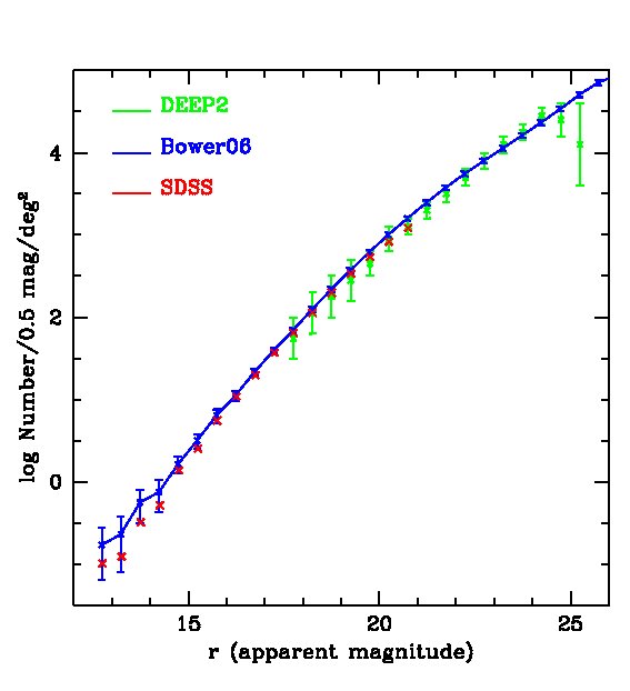
Since neither the nor the -band coincide with any of the PS1 bands, for a more direct test we compare predicted galaxy number counts in the -band with data. At the faint end we use the number counts over 5 sq deg from the deep2 survey (Coil et al., 2004), which are complete to 24.75 in the band. To minimise sample variance at the bright end, we use galaxy number counts in the SDSS commissioning data (Yasuda et al., 2001) which cover about 440 sq deg and are complete to . (We have checked that the difference between the commissioning data and more recent SDSS releases (Fukugita et al., 2004; Yasuda et al., 2007) is negligible). We compute the galform model predictions, including uncertainties, from 10 realizations of 10 sq deg mock surveys. The results, displayed in Fig. 2, show that our model prediction agrees very well with both the deep2 and the SDSS datasets. Note that we have applied the 0.15 magnitude shift discussed in §2.2 to the model galaxies.
3.3 Expected PS1 galaxy numbers counts and redshift distributions
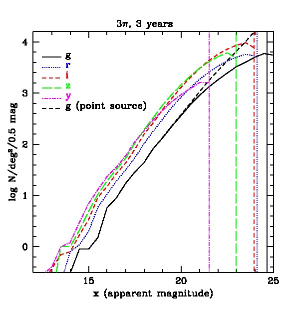
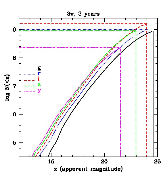
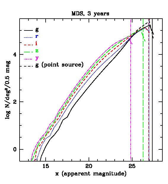
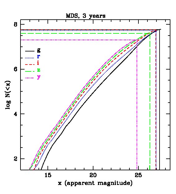
We now discuss the expected population statistics for the PS1 surveys predicted by our mock catalogues. We apply Petrosian magnitude cuts in each of the PS1 bands and plot the expected galaxy number counts in 0.5 magnitude bins in Fig. 3, for both the 3-year survey and the MDS. The figure shows that, with the Petrosian magnitude cuts, the samples are no longer complete to the 5 point source magnitude limits in the various bands, but rather only to 2 magnitudes brighter. Note that the -band magnitude limit is substantially shallower than the others and so, if one requires detection in all five bands, the limit is the most restrictive.
The cumulative distributions on the right hand panels of Fig. 3 reveal the staggering number of galaxies that will be detected by PS1. For example, in the -band after 3 years, we expect about galaxies in the 3 survey and nearly in the MDS.
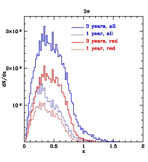
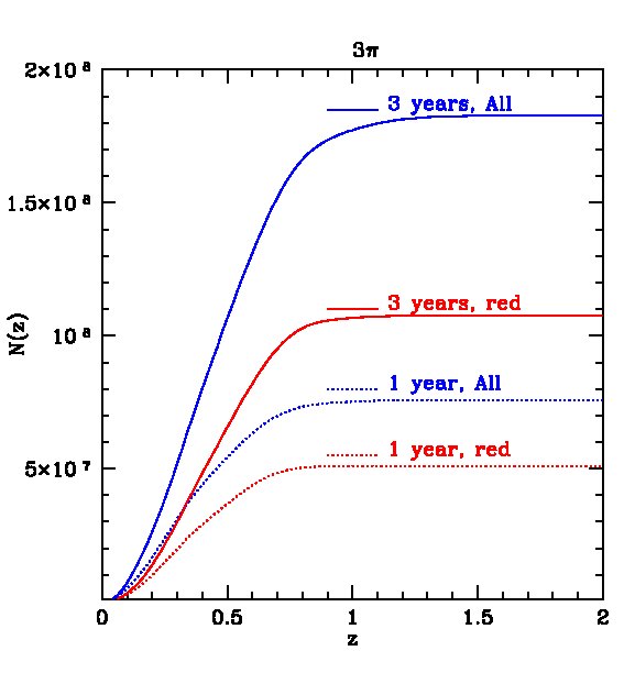
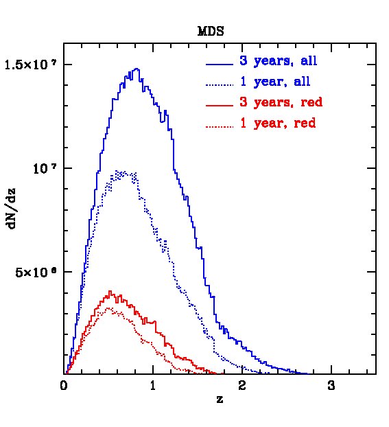
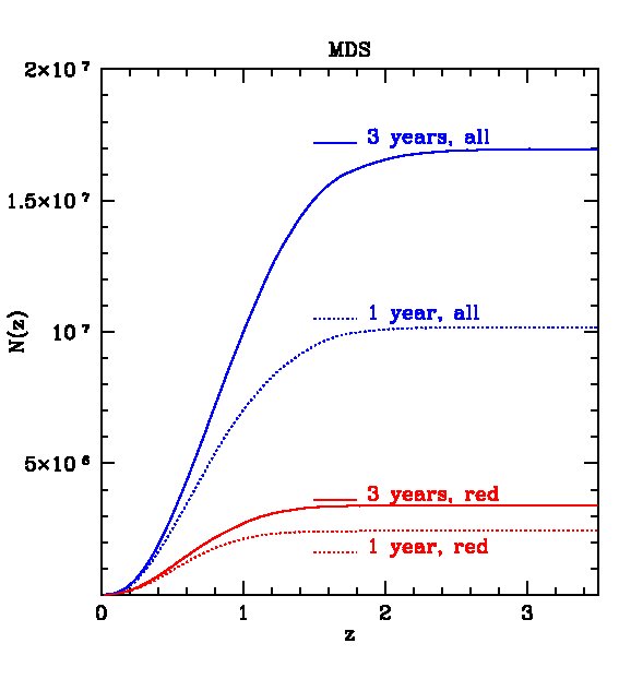
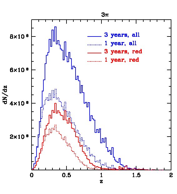
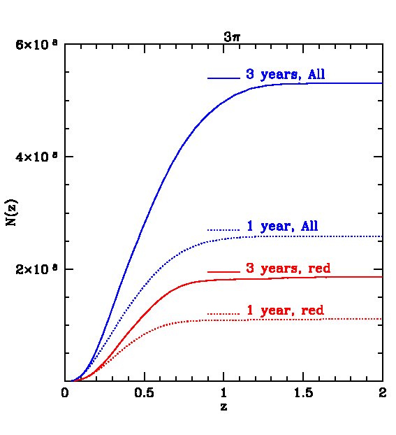
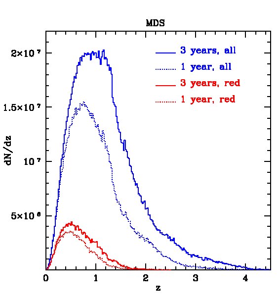
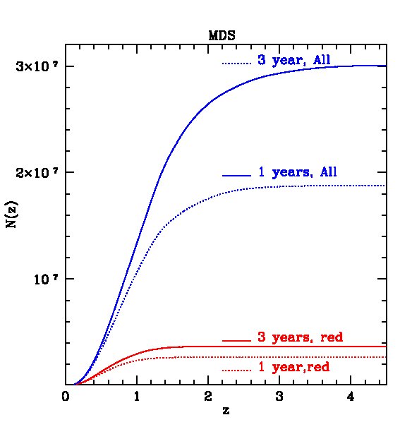
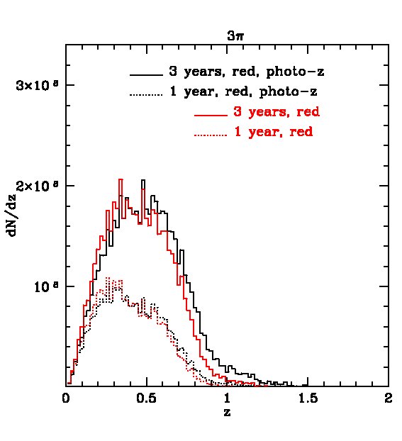
The expected redshift distributions for the two surveys are shown in Fig. 4 for galaxies detected in all 5 bands and in Fig. 5 for galaxies detected only in and , i.e. not requiring the shallow -band detection. In the first case, the distribution peaks at for the survey, with about and galaxies detected (in all 5 bands) in the 1- and 3-year surveys respectively. The survey is so huge, that, after 3 years, we expect about 10 million galaxies at and 5 million at . For the MDS survey, the distribution peaks at , with a total of galaxies after 3 years of which around 0.5 million lie at . Removing the -band constraint leads to a large increase in the number of galaxies, as shown in Fig. 5. In this case, the survey will contain galaxies after three years, with about 30 million at , while the MDS will contain galaxies, with 4 million at .
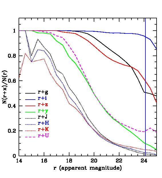
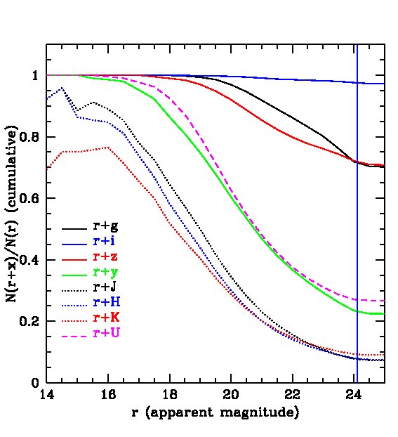
For certain applications, for example, for the estimate of photometric redshifts discussed in the next section, it might be desirable to supplement the PS1 filter system with other bands, particularly in the near infrared. The UKIDSS Infrared Deep Sky Survey (e.g. Lawrence et al., 2007; Hewett et al., 2006) is particularly relevant in this context. The UKIDSS Large Area Survey (LAS) aims to map about 4000 sq deg of the Northern sky (contained within the survey) over the course of a few hundred nights. The Deep Extragalactic Survey (DXS) aims to cover 35 square degrees of the sky in three separate regions which have a large overlap with the fields chosen for the MDS. Details of the , and magnitude limits of the UKIDSS surveys are listed in Table 2. In order to assess the compatibility of the PS1 and UKIDSS surveys, we show in Fig. 6 the reduction in galaxy counts, relative to a pure -band selection, that would result from combining in turn each of the filters with the -band filter. We see, once again, that the -band cut (green line) is much shallower than the other PS1 bands. The UKIDSS (LAS) and bands are even shallower. Combining -band and -band detections also results in a large reduction in the counts even for an optimistic -band limit of 23 mag. Fig. 6 suggests that, in spite of the large area overlap with the survey, the UKIDSS (LAS) survey may be too shallow to pick up PS1 galaxies at high redshifts. It will be very difficult for a -band survey to pick up a significant number of PS1 galaxies.
4 Photometric redshifts in the PS1 survey
We now examine the accuracy with which redshifts are likely to be estimated using PS1 photometry. For this purpose we adopt an off-the-shelf photometric redshift code, the Hyper- code of Bolzonella et al. (2000) which is based on fitting template spectra. We do not attempt to tune the performance of the estimator in anyway, and so our results should perhaps be regarded as providing a pessimistic view of the photometric redshift performance of PS1. Once PS1 data become available, bespoke estimators will be developed which are optimized to return the smallest random and systematic errors for the PS1 filter set and galaxies by having empirically adaptive galaxy templates (e.g. Bender et al., 2001).
The basic principle behind the template fitting approach to photometric redshift estimation is the following. The observed SED of a galaxy is compared to a set of template spectra and a standard minimisation is used to obtain the best fit:
| (9) |
where , and are the observed fluxes, template fluxes and the uncertainty in the flux through filter , respectively and is a normalization factor. For the fitting procedure, we input the PS1 -band filter transmission curves and, when appropriate, those of the UKIDSS near infrared bands and a band filter. We consider different reddening laws and two sets of model templates: the mean spectra of local galaxies given by Coleman et al. (1980, CWW) and the synthetic spectra given by Bruzual & Charlot (1993, BC). We set a redshift range of for the 3 and for the MDS sample.
One might be concerned that the use of Bruzual & Charlot stellar population synthesis models to generate both the template spectra and the galaxy spectra in the mock catalogues might lead to an underestimate of the error on the photometric redshift. There are two key differences between the mock spectra and the templates which mean that this is not an issue: i) the complexity of the composite stellar populations of mock galaxies and ii) the differing treatments of dust extinction. The template spectra correspond to a single parameter star formation history (characterized by an exponentially decaying star formation rate, where the -folding time is treated as a parameter) and a fixed metallicity for the stars. The mock galaxies, on the other hand, have complicated star formation histories which cannot be fitted by a decaying exponential (see Baugh 2006 for examples of star formation histories predicted by the semi-analytical models). Furthermore, the stars in the mock galaxy have a range of metallicities. Hyper-, in common with many other photometric redshift estimators, assumes that dust forms a foreground screen in front of the stars with a particular extinction law. In galform, the dust and stars are mixed together. This more realistic geometry can lead to dust attenuation curves which look quite different from those assumed in the photometric redshift code (Granato et al., 2000).
The Hyper- code calculates a redshift probability distribution, , for each galaxy. Because of a degeneracy between the 4000 and the 912 breaks, the shape of can have a double peak, causing some low redshift galaxies to be misidentified as high redshift galaxies and viceversa. Some of these misidentifications can be removed by applying extra constraints, for example, the galaxy luminosity function and the differential comoving volume as a function of redshift (Mobasher et al., 2007). For a given observed flux, both these functions provide an estimate of the probability that the galaxy has redshift which can be use to modulate . The highest peak in the combined probability distribution gives the best estimate of the photometric redshift. We use the -band luminosity function of the B06 model for this purpose.
We now discuss how the accuracy and reliability of the photometric redshift estimates depends on various choices. We do this by calculating photometric redshifts for a 10 sq deg subsample of our mock PS1 3-year catalogue and comparing these with the true redshifts (which we will sometimes refer to as the “spectroscopic” redshifts.)
1. Choice of SED template (CWW vs BC)
Our tests show that using 5 input spectral types: burst, S0, Sa, Sc and Im, gives good results; adding more spectral types does not produce further significant improvement. We find that fitting with the CWW templates gives larger statistical uncertainties and systematic deviations from the true redshift than fitting with the BC templates, especially at high redshift (). The reason for this could be that the CWW templates are based on observations of the local universe and may not be sufficiently representative of galaxies at high redshift. In what follows, we will exclusively use the BC templates.
We also experimented with BC templates for different metallicities. Because of the age-metallicity degeneracy in galaxy SEDs, we did not find any improvement by allowing the metallicity to vary while letting the age of the stellar populations be a free parameter. Since the 4000 break only becomes detectable after a stellar population has aged beyond years, we exclude templates with ages smaller than this. This greatly improves the results for low redshift galaxies ().
2. Dependence on photometric bands
The accuracy of the redshift estimates depends on the choice of photometric bands. With our 10 sq deg 3-year mock catalogues, we can explore which combination of bands gives optimal results for PS1. We have considered many combination of the PS1 photometry with UKIDSS (LAS) and fiducial and photometry. Note that, if the flux through any of the , , , or filters drops below the 5 flux limit, the noisy measured flux is still used with its appropriate uncertainty.
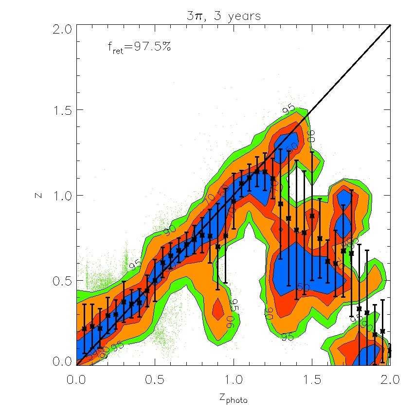
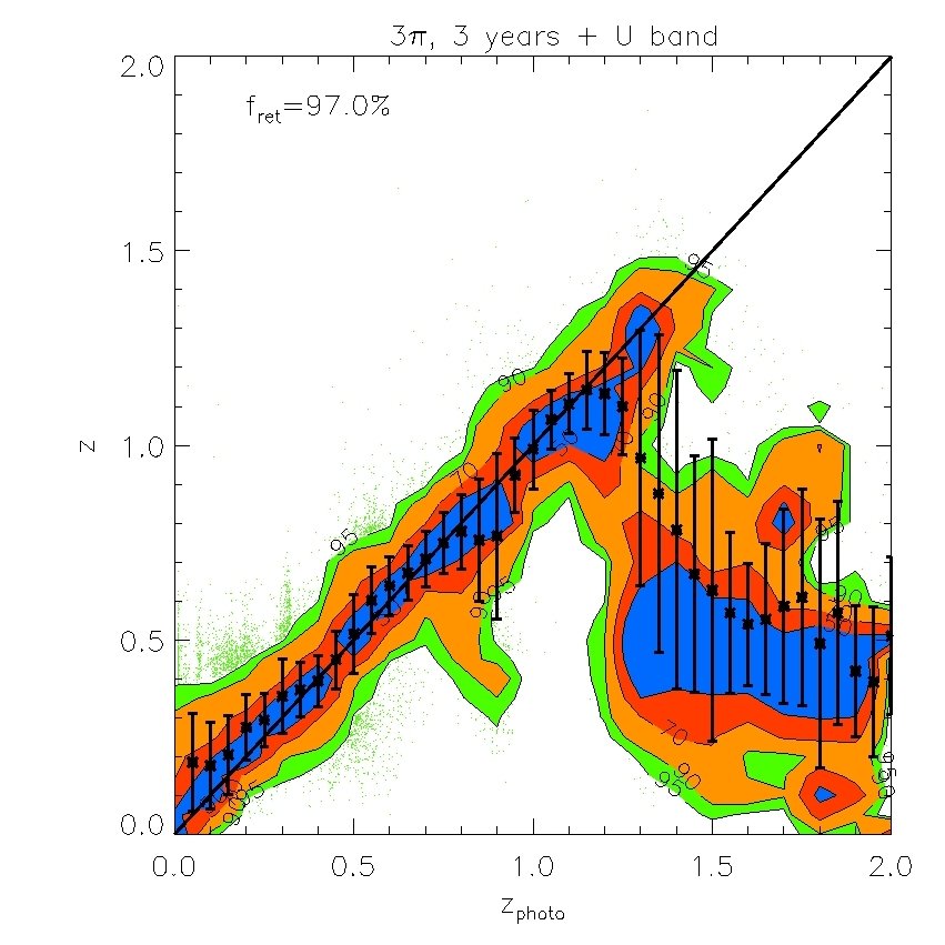
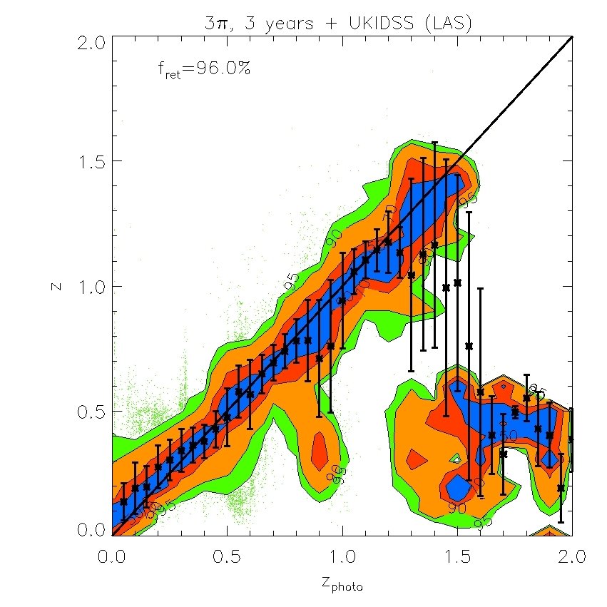
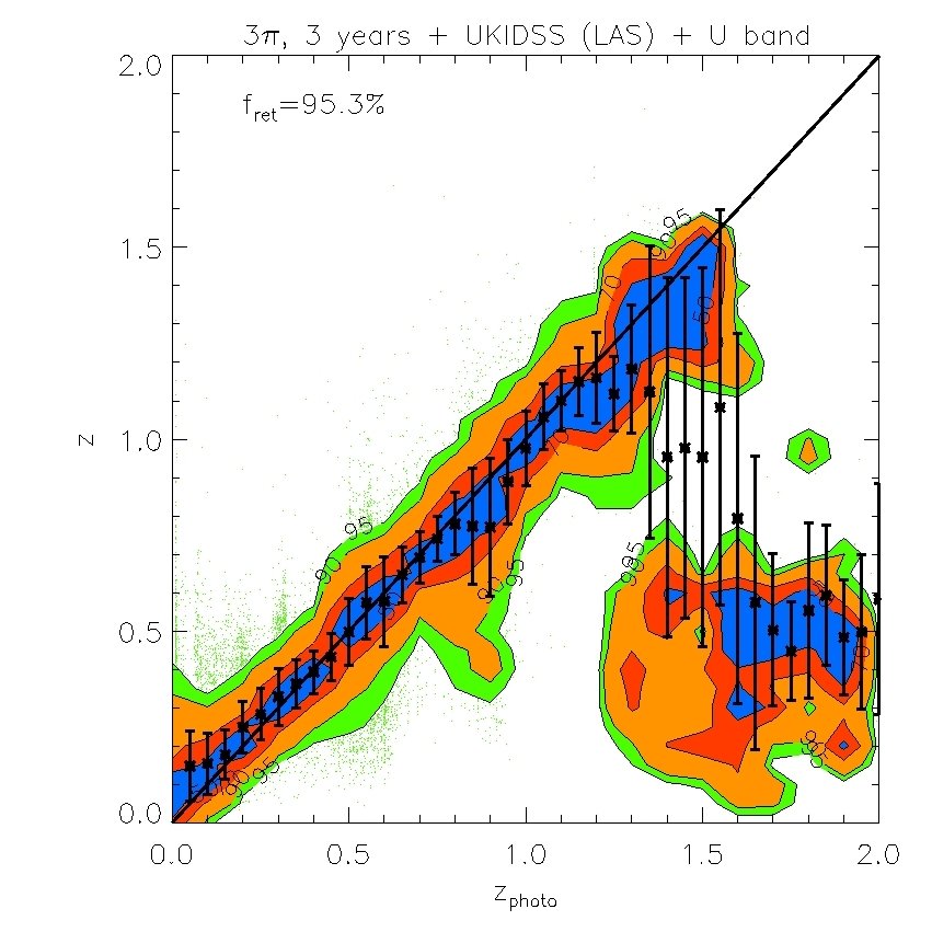
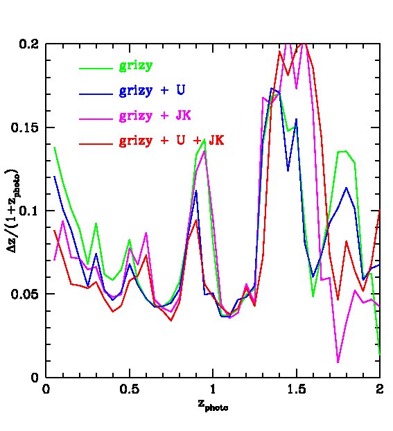
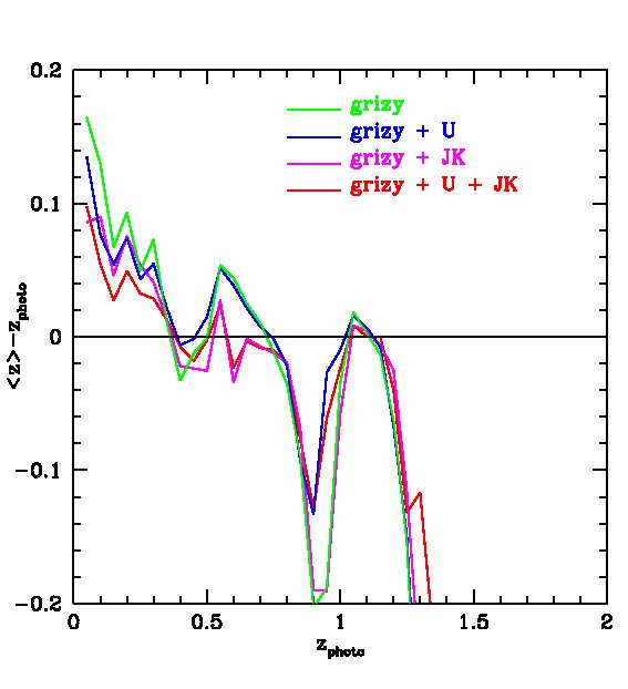
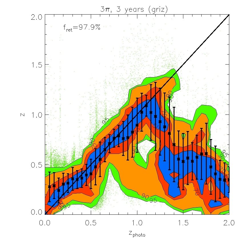
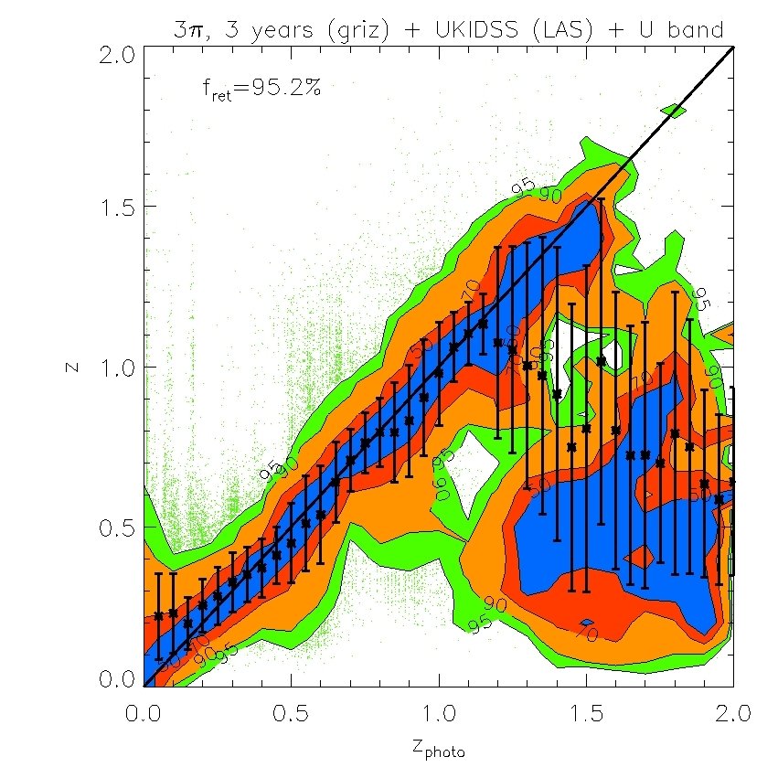
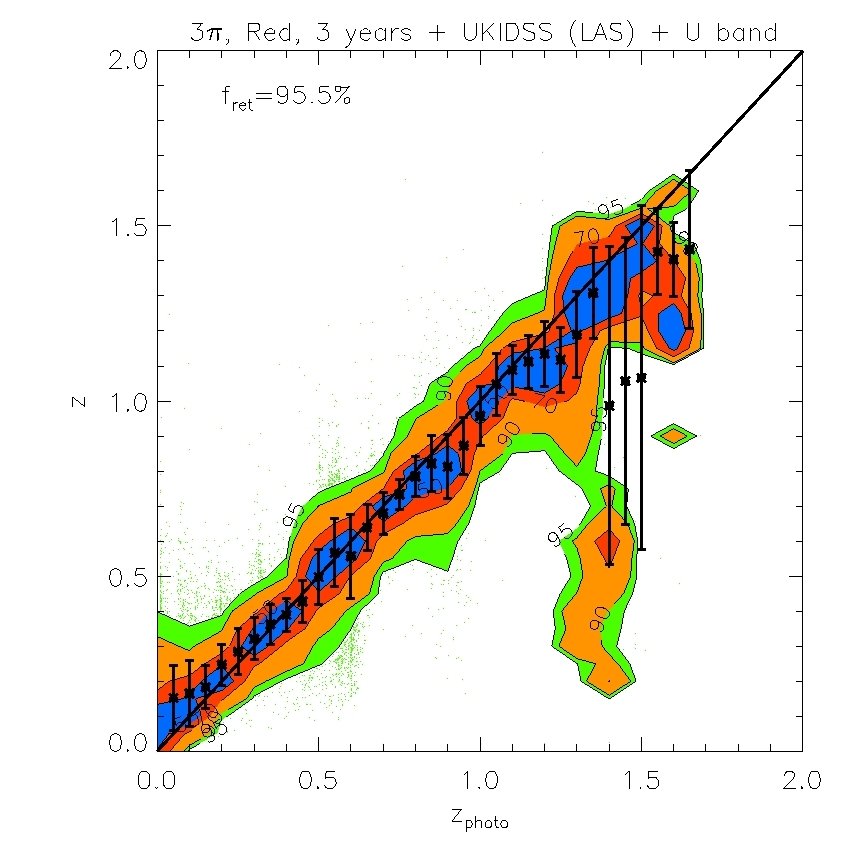
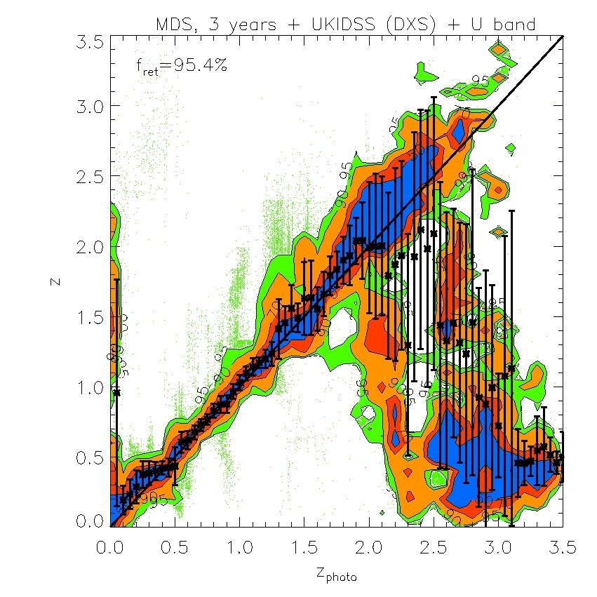
We find that the -band (whose effective wavelength is very close to the band) does not improve the fits if is available, but the -band is still useful even when -band data are included. We also find that the -band is not important provided and are available. However, both and are important for improving the quality of the fits. Therefore, in what follows we will ignore and . Our results are displayed in Figs. 7 and 8. In Fig. 7, we plot the “spectroscopic” redshifts against our estimated photometric redshifts for the 4 cases above. For clarity, rather than plotting each galaxy on these plots, we have instead displayed contours that indicate the region in each bin of photo- that contains 50%, 70%, 90% and 95% of the galaxies. Galaxies with “spectroscopic” redshifts falling outside the contours are shown individually by green dots. To evaluate the scatter we eliminate extreme outliers through standard 3 clipping. Typically over of the galaxies are retained, as indicated in the legend. Fig. 7 plots the true or “spectroscopic” redshift against our estimated photometric redshift for the PS1 photometry alone and when supplemented by -band photometry, UKIDSS (LAS) photometry, or both. Fig. 8 (left panel) shows plotted against redshift where is the error from Fig. 7. The bias in the mean of each redshift bin relative to the true value is also shown (right panel).
The PS1 bands alone give relatively accurate photometric redshifts in the range , with typical rms values of . The random and systematic errors increase at both lower and higher redshifts and there is a population of low redshift () galaxies which are incorrectly assigned high redshifts. Adding the -band produces only a moderate improvement at all redshifts. Using both the and bands results in a significant improvement at , but not at higher redshifts. Finally, combining the , and , produces the best results. For this best case, the rms error, , in the range and, for , it is never larger than 0.15.
We saw in §3.3 that requiring that galaxies be detected in , the shallowest PS1 filter, reduces the sample size by factors of 2-3. The deeper sample that we achieve by only requiring detections has significantly less accurate photo-s. This is shown in Fig. 9, in which we measure photometric redshifts using only photometry. In this, the rms in the redshift range increases from to and the bias changes little.
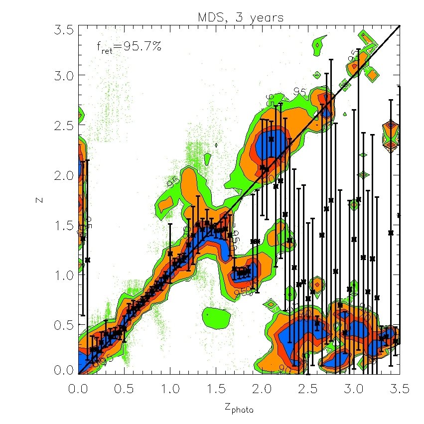
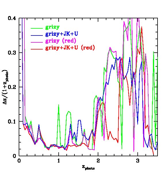
Photometric redshift estimates for the MDS are shown in the top 2 panels of Fig. 12 and their accuracy is quantified by the green and blue lines in Fig. 13. If only the PS1 are available, an accuracy of is achievable for . Adding the UKIDSS (DXS) and the -band improves the estimates considerably, but there is still a clear bias at very low and high redshifts. This is mainly because the depths of the UKIDSS (DXS) and our assumed band is insufficient to match the depth of the MDS so faint galaxies are not detected in the UKIDSS and band nor in the band.
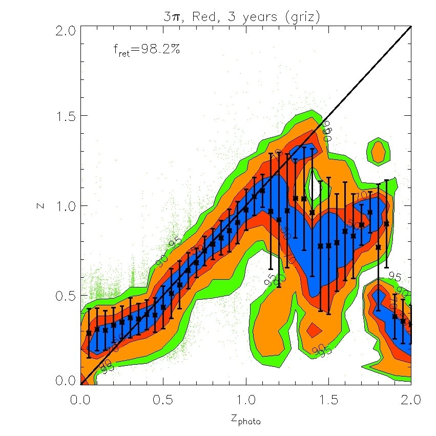
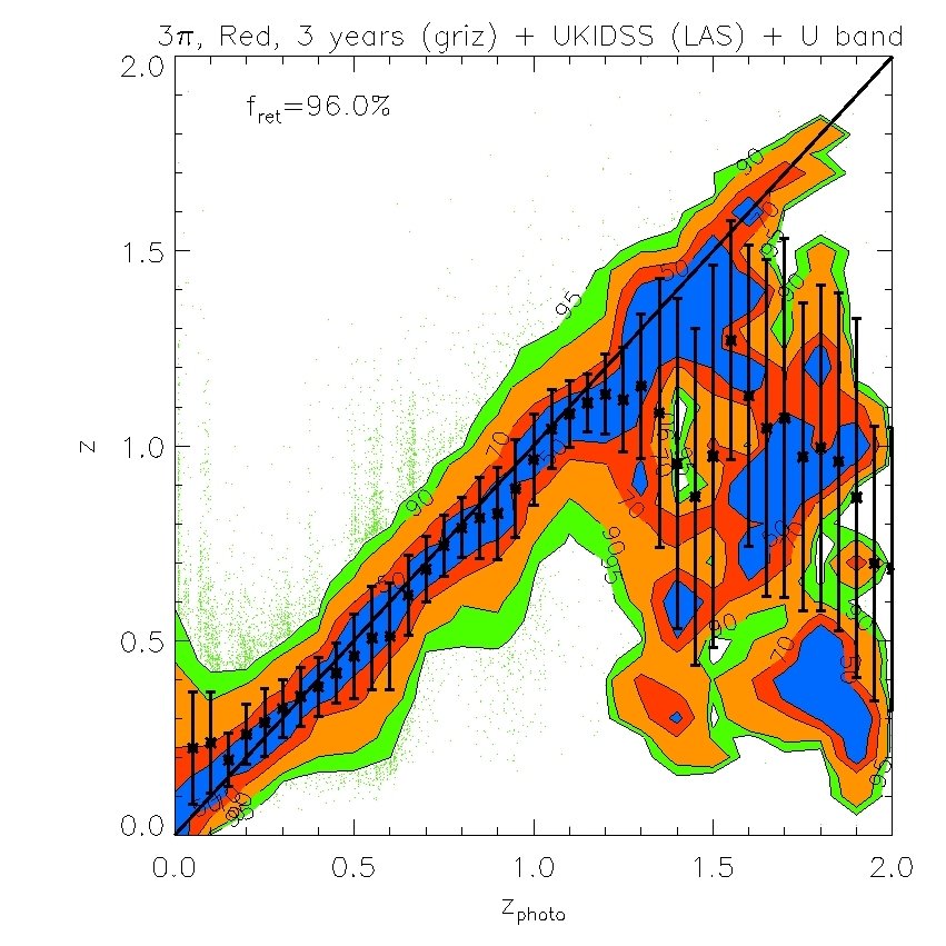
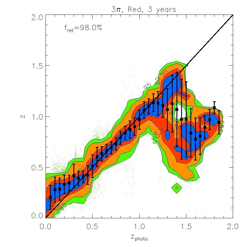
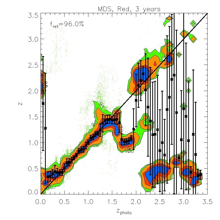
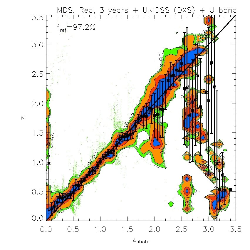
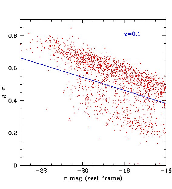
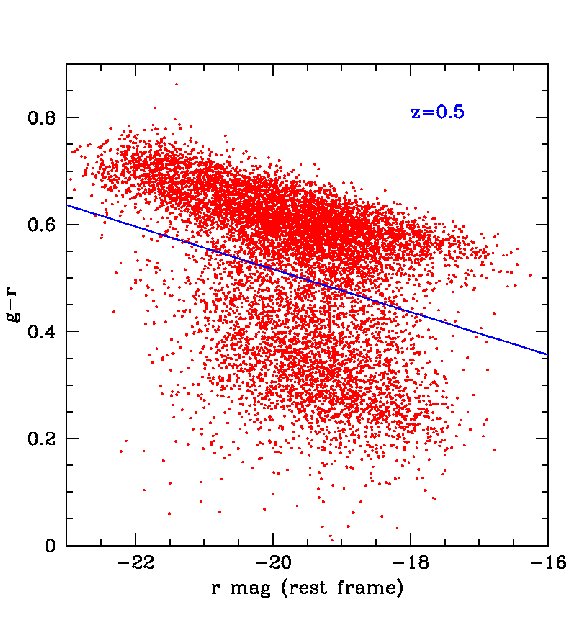
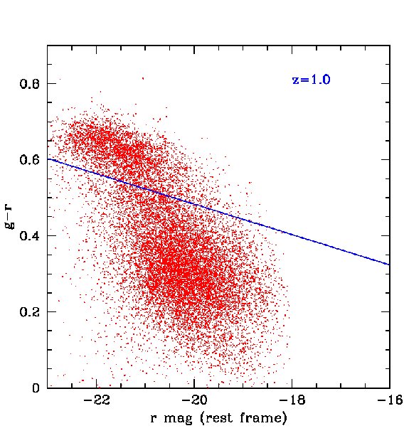
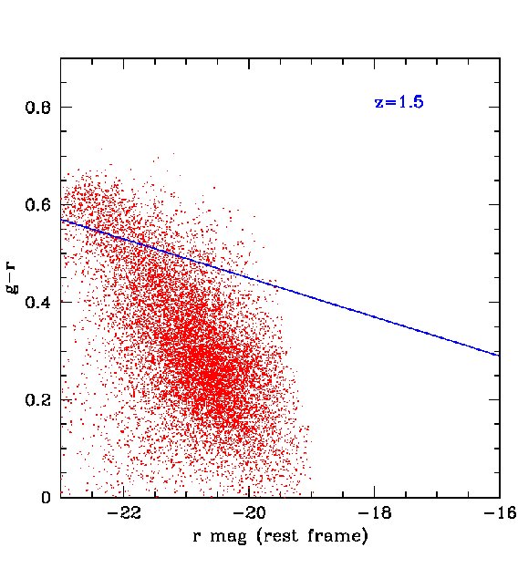
For certain applications, for example, the measurement of baryonic acoustic oscillations discussed in the next section, smaller rms errors than those found above are required. These can be achieved by selecting subsamples of galaxies whose spectra are particularly well suited for the determination of photometric redshifts, such as red galaxies which have strong 4000 breaks. The most direct way to define a red subsample is by using the rest frame colours. In Fig 14, we plot the predicted rest-frame against -band luminosity at four different redshifts in our mock MDS catalogue. A cut at neatly separates out the red sequence, particularly at . The redshift distributions of red galaxies defined this way are shown by the red lines for both the 3 survey and the MDS in Figs. 4 and 5. The distributions peak at slightly lower redshifts than the full samples, but there is still an impressive number of red galaxies in the two surveys. For example, in the 3 survey we expect about 200 million galaxies after 3-years if detection in is not required or 100 million if it is.
In practice, rest-frame colours are difficult to estimate from the observations. An alternative method for identifying red galaxies is to use the spectral type determined by Hyper-. We define a red sample by the following criteria, galaxies which are best fit with the ‘Burst’ spectral type and a stellar population older than yr.
Fig. 15 shows the redshift distribution for this sample which can be seen to be very similar to the redshift distribution of a red sample selected by rest-frame colour. This suggests that it will be possible to select a red galaxy sample directly from the observational data alone.
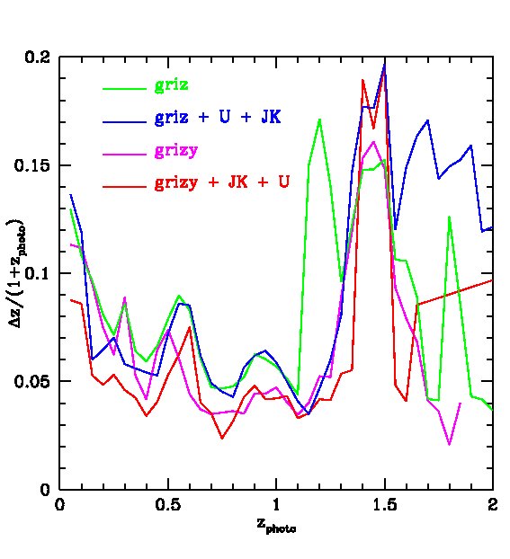
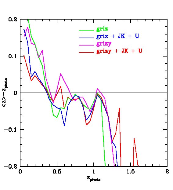
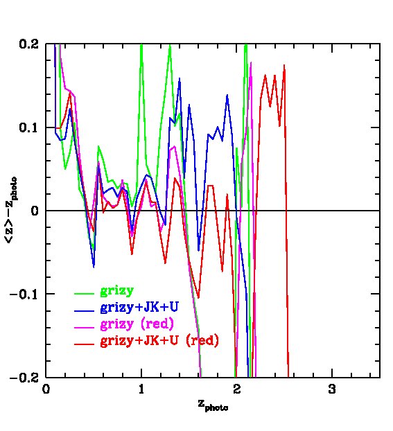
Fig. 10 and Fig. 12 show photometric redshift estimates for red galaxies in the 3-year 3 survey and the MDS respectively. Their accuracy is illustrated by the magenta ( photometry only) and red lines (++) in Figs. 11 and Fig. 13 respectively. Results without the -band photometry are shown in the top panels of Fig. 10 and in green ( photometry only) and blue (++) lines in Fig. 11. These figures show the dramatic improvement in photometric redshift accuracy for red galaxy samples. For example, for the survey, the rms value of can be as low as 0.02 at when combining with UKIDSS (LAS) and bands measurements. Similarly, in the MDS with the same combination of filters, the accuracy for red galaxies is much higher than for the sample as a whole and can be as good as in the redshift range .
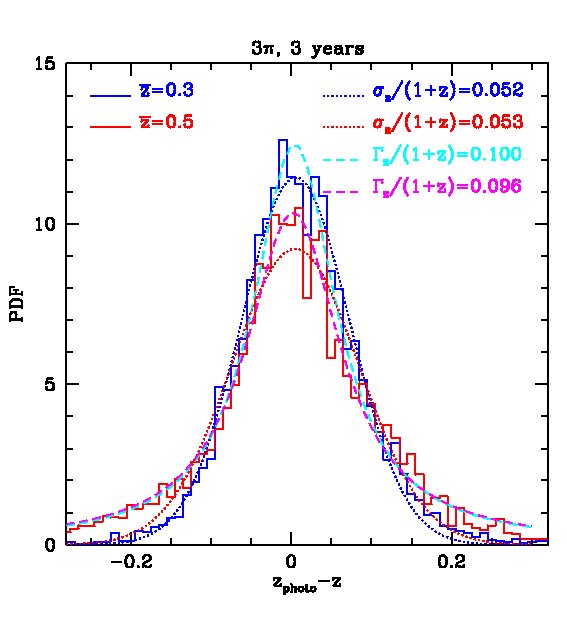
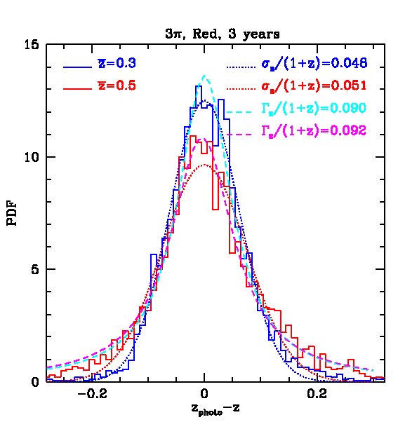
Finally, we consider the form of the distribution of the photo- errors in Fig. 16. The photo- error distributions are well fitted by a Gaussian function, with variance . The error distribution could also be equally well fitted by a Lorentzian function. Example distributions are shown at and in Fig. 16. An application of our results for the size and form of the photo- errors is presented in the next section, in which we investigate their effect on the baryonic acoustic oscillation measurements.
5 Implications for BAO Detection
In this section we investigate the impact of using photometric redshifts on the accuracy with which the baryonic acoustic oscillation (BAO) scale can be measured from the power spectrum of galaxy clustering. BAOs have been proposed as a standard ruler with which the properties of the dark energy may be measured (Blake & Glazebrook, 2003; Linder, 2003). Our aim here is to provide a simple quantification of the factor by which the effective volume of a survey is reduced when photometric redshifts are used in place of spectroscopic redshifts. This will provide a rule of thumb indicator of the relative performance of photometric and spectroscopic surveys for the measurement of BAO. We defer a more extensive treatment of the full impact of the survey window function on the measurement of BAOs to a later paper. Mocks with clustering will play an important role in assessing the optimal way to measure the clustering signal in photometric surveys.
The photometric redshift technique allows large solid angles of sky to be covered to depths exceeding those accessible spectroscopically at a low observational cost. However, the inaccurate determination of a galaxy’s redshift results in an uncertainty in its position and this leads to a distortion in the pattern of galaxy clustering. We shall refer to a measurement of the power spectrum which uses photometric redshifts to assign radial positions as being in “photo-” space.
The errors introduced by photometric redshifts can be modelled as random perturbations to the radial positions of galaxies. As we have found from our photo- measurements that the photo- errors can be well fitted by a Gaussian function, if we assume that these perturbations are Gaussian distributed with mean equal to the true redshift and width , then the Fourier transform of the measured density field, , can be written as
| (10) |
where , is the line-of-sight direction and is the density field measured in redshift space. From this expression, the spherically averaged power spectrum can be approximately111It is an approximate expression since the redshift space distortions and photometric redshift errors do not commute under a spherical average (see Peacock & Dodds, 1994). written as:
| (11) |
where is the error function. In addition, the power spectrum in photo- space can be seen as that in redshift space with additional damping on small scales due to the large value of . On very large scales the main contribution to the power spectrum comes from modes with wavelengths larger than the typical size of the photometric redshift errors. Therefore, the clustering on these scales is essentially unaffected. On the contrary, on scales comparable to and smaller than the photo- errors, structures are smeared out along the line-of-sight. The modes describing these scales along the line-of-sight contain little information about the true distribution of galaxies and contribute only noise to the power spectrum.
We investigate these effects directly on the measurement of the matter power spectrum using large N-body simulations. We use the l-basicc ensemble of Angulo et al. (2008), which consists of 50 low-resolution, large volume simulations. Each has a volume of and resolves halos more massive than . The assumed cosmological parameters are , , , and . Their huge volume makes the l-basicc simulations ideal to study the detectability of BAO in future surveys. Photometric redshift errors are mimicked as a random perturbation added to the particles’ position along one direction (line-of-sight). The perturbations are drawn from a Gaussian distribution with various widths representing different degrees of uncertainty in the photometric redshift. Despite their large volume, the l-basicc boxes are more than an order of magnitude smaller than the volume which will be covered by the survey. Hence, we present results for the relative change expected in the random errors for different photometric redshift errors. Angulo et al. found that any systematic error in the recovery of the BAO scale was comparable to the sampling variance between l-basicc realizations. To address the question of systematic errors we will need to use even larger volume simulations. Furthermore, new estimators are likely to be developed to extract the optimal BAO signal from photometric surveys. These more detailed questions are deferred to a later paper.
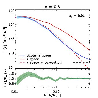
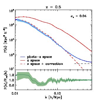
In the upper panels of Fig. 17 we show the mean, spherically averaged power spectrum of the dark matter measured from the l-basicc simulations at , along with its variance, in photo- space (solid blue lines). The size of the photo- errors are and (equivalent to and Mpc at ) in the left- and right-hand panels respectively. We have also plotted the power spectrum measured in redshift-space (solid red lines) and the analytical expression of Eq. 11 (dashed red line). By comparing the spectra in redshift and photo- spaces, the additional damping described above is evident. Also, we see that Eq. 11 describes quantitatively this extra damping on scales where the power spectrum is not shot-noise dominated.
In the lower panels of Fig. 17 we take a closer look at the BAO by isolating them from the large-scale shape of the power spectrum. We do this by dividing the power spectrum by a smoothed version of the measurement. It is clear that since the number of “noisy modes” increases with the size of the photometric redshift errors, the error on the power spectrum and therefore on the BAO also increases. The visibility of the higher harmonic BAO is also reduced as the photometric redshift error increases. In order to quantify the loss of information, we have followed a standard technique to measure BAO as described in Angulo et al. (2008) (see also Percival et al., 2007 and Sanchez et al., 2008). The method basically consists of dividing the measured power spectrum by a smoothed version of the measurement. In this way, any long wavelength gradient or distortion in the shape of the power spectrum is removed which diminishes the impact of possible systematic errors due to redshift space distortions, galaxy bias, nonlinear evolution and, in the case described in this paper, photometric redshift distortions. Then, we construct a model ratio using linear perturbation theory, , which we fit to the measured ratios. In the fitting procedure there are two free parameters: (i) a damping factor to account for the destruction of BAO peaks located at high by non-linear effects and redshift-space distortions and (ii) a stretch factor, , which quantifies how accurately we can measure the BAO wavelength. The latter gives a simple estimate of how well we can constrain the dark energy equation of state from BAO measurements alone.
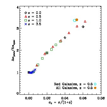
Fig 18 shows the results of applying our fitting procedure to the l-basicc ensemble at different redshifts. On the -axis we plot the size of the photometric redshift error divided by , whilst on the -axis we plot the predicted error on divided by the error we infer for an ideal spectroscopic survey (i.e. from the power spectrum in redshift-space). Since the error on scales with the error on the power spectrum and the latter is proportional to the square root of the volume of the survey, the -axis should be roughly equal to the square root of the factor by which the volume of a photometric redshift needs to be larger than the volume of a spectroscopic survey to achieve the same accuracy.
Several authors have investigated the implications of photometric redshift errors on the clustering measurements in general and on the BAO in particular (Seo & Eisenstein, 2003; Amendola et al., 2005; Dolney et al., 2006; Blake & Bridle, 2005). Our analysis improves upon these studies in several ways: (i) we have included photometric redshift errors directly into an realistic distribution of objects; (i) by using N-body simulations, our calculation takes into account the effects introduced by nonlinear evolution, nonlinear redshift-space distortions and shot noise; (iii) the use of 50 different simulations enables a robust and realistic estimation of the errors on the power spectrum measurements; (iv) we have investigated how our results change if we use the actual distribution of photometric redshift errors (the cyan and brown circles in Fig 18), instead of a Gaussian fit and we find only a small additional degradation.
These improvements lead to predictions that are somewhat different from previous ones. For example, for , Blake & Bridle (2005) predict a factor of 10 for the reduction of the effective volume of a photometric survey. Here, as shown in Fig. 18, we find a reduction which is a factor 2 times smaller than this (i.e. a volume reduction factor of 5). The main difference between our analyses is that Blake & Bridle (2005) use only modes larger than , arguing that wavelengths shorter than the size of the photometric redshift errors contribute only noise. In reality, there is a smooth transition around , with signal coming from all wavenumbers (with different weighting, of course). In addition, the neglect of nonlinear evolution (which erases the BAO at high wavenumbers) also contributes to Blake & Bridle (2005) overestimating the reduction in effective volume. These two effects together explain the disagreement between our results.
6 Discussion and conclusions
We have described a method for constructing mock galaxy catalogues which are well suited to aid in the preparation, and eventually in the interpretation of large photometric surveys. We applied our mock catalogues specifically to the data that will shortly begin to be collected with PS1, the first of the 4 telescopes planned for the Pan-STARRS system.
Our mock catalogue building method relies on the use of two complementary theoretical tools: cosmological N-body simulations and a semi-analytic model of galaxy formation. For this study, we have employed the Millennium N-body simulations of Springel et al. (2005) together with galaxy properties calculated using the galform model with the physics described by Bower et al. (2006). Although this model gives quite a good match to the local galaxy luminosity function in the B- and K-band, we refined the match by applying a small correction of 0.15 mag to the luminosities of all galaxies, so that the agreement with the SDSS luminosity function is excellent. Similarly, we applied a correction to the predicted galaxy sizes as a function of redshift in order to match the SDSS distribution of Petrosian half-light radii in the -band. As a simple test, we showed that our galaxy formation model agrees very well with the -band number counts in the SDSS Commissioning and deep2 data over a range of 12 magnitudes.
We adopt a similar magnitude system as the SDSS, based on the use of Petrosian magnitudes and use these to calculate the expected magnitude limits for extended objects in the two surveys that PS1 will undertake, the “3” survey and the MDS. We find that, after 3 years, the 3 survey will have detected galaxies in all 5 photometric bands ( and ), with a peak in the redshift distribution of 0.5 and an extended tail containing about 10 million galaxies with . The MDS will detect galaxies, the redshift distribution peaking at , with 0.5 million galaxies lying at . Of the 5 PS1 bands is the shallowest and removing the requirement that a galaxy be detected in this band more than doubles the total numbers in the sample.
We have used our mock catalogues to take a first look at the accuracy of photometric redshifts in the PS1 photometric system. Photometric redshifts can be readily estimated using the public Hyper- code of Bolzonella et al. (2000). With the PS1 bands alone it is possible, in principle, to achieve an accuracy in the 3 survey of in the range . This could be reduced to 0.05 by adding and photometry from the UKIDDS (LAS) and could be improved even further with a hypothetical band survey to 23 mag, although the samples become progressively smaller as these additional bands are added. Cutting at the relatively shallow depth of the -band is important in achieving these errors. Going deeper than the -band data would increase the sample size substantially, but the errors would increase to 0.075. There is therefore a balance to be struck between reducing the sample size (by about a factor of 2) which increases the accuracy of all the photometry, allows the -band to be used and has the combined effect of increasing the photometric redshift accuracy. For the MDS an accuracy of is achievable for using the PS1 bands alone, with similar fractional improvements as for the 3 survey by the inclusion of and near infrared bands.
A dramatic improvement in photometric redshift accuracy can be achieved for samples containing only red galaxies. We have shown that it should be possible to identify a red sample (i.e. with red rest-frame colours) directly from the photometric data using the best-fit Hyper- templates. These samples can still contain large numbers of galaxies. For example, an accuracy of may be achievable for 100 million red galaxies at in the 3 survey. Similarly, for the MDS, this sort of accuracy could be achieved for 30 million galaxies at . These estimates are all based on the “off-the-shelf” Hyper- code, without any tuning of the code for the PS1 setup. We expect that further improvements should be possible by refining the photometric redshift estimator and tailoring it specifically to the PS1 bands.
Our analysis is based on the use of the galform semi-analytic galaxy formation model. Although this model gives a good match to a large range of observed galaxy properties, it is based on a number of approximations and has uncertain elements which could be relevant to the estimation of photometric redshifts. These include the effects of reddening, assumptions about the frequency and duration of bursts and the use of the Bruzual & Charlot (1993) stellar population synthesis libraries which are the same as assumed in our implementation of Hyper-. We note that the star formation histories predicted by the model are much more varied and have a richer structure than those assumed to construct the Hyper- templates, and that the treatment of dust extinction is very different in galform. Abdalla et al. (2008) carried out a similar study to ours and reached similar conclusions about the size of the photometric redshift errors and the usefulness of additional filters in the NIR or far-UV. This is encouraging as Abdalla et al. used a completely different photometric redshift estimator, ANNz, an artificial neural network code written by Collister & Lahav (2004). Furthermore, instead of using a galaxy formation model to generate a mock catalogue, these authors used a mixture of empirical and theoretical techniques to produce a set of galaxies on which to test their estimator.
One of the main applications of the PS1 3 survey will be to the determination of the scale of baryonic acoustic oscillations used to constrain the properties of the dark energy. We have investigated how uncertainties in the photometric redshifts will degrade the determination of the BAO scale and, in particular, we have quantified the factor by which the effective volume of a photometric survey is reduced by these uncertainties. We find that, with the sorts of photometric redshift uncertainties that we have estimated for a red sample, PS1 will achieve the same accuracy as a spectroscopic galaxy survey containing 1/5 as many galaxies. Unfortunately, spectroscopy for 20 million galaxies at is not likely to be feasible for some time. PS1 should be able to provide competitive estimates of the BAO scale in the next few years.
ACKNOWLEDGEMENT
YC is supported by the Marie Curie Early Stage Training Host Fellowship ICCIPPP, which is funded by the European Commission. This work was supported in part by the STFC Rolling Grant to the ICC for research into “The growth of structure in the Universe.” REA is supported by a STFC/British Petroleum sponsored Dorothy Hodgkin postgraduate award. CMB is funded by a Royal Society University Research Fellowship. CSF acknowledges a Royal Society Wolfson Research Merit Award. We acknowledge helpful comments from Stef Phleps and the OPINAS-LSS group and Dave Wilman which helped to improve the presentation of an earlier draft. We also acknowledge useful comments from Richard Bower, Ken Chambers, Alan Heavens, Bob Joseph, Peder Norberg, John Peacock and Tom Shanks.
References
- Abdalla et al. (2008) Abdalla F. B., Amara A., Capak P., et al. 2008, MNRAS, 387, 969
- Almeida et al. (2007) Almeida C., Baugh C. M., Lacey C. G., 2007, MNRAS, 376, 1711
- Amendola et al. (2005) Amendola L., Quercellini C., Giallongo E., 2005, MNRAS, 357, 429
- Angulo et al. (2008) Angulo R. E., Baugh C. M., Frenk C. S., Lacey C. G., 2008, MNRAS, 383, 755
- Baugh (2006) Baugh C. M., 2006, Reports of Progress in Physics, 69, 3101
- Baugh et al. (1996) Baugh C. M., Cole S., Frenk C. S., 1996, MNRAS, 283, 1361
- Baugh et al. (2005) Baugh C. M., Lacey C. G., Frenk C. S., Granato G. L., Silva L., Bressan A., Benson A. J., Cole S., 2005, MNRAS, 356, 1191
- Bender et al. (2001) Bender R., Appenzeller I., Böhm A., 2001, in Cristiani S., Renzini A., Williams R. E., eds, Deep Fields. Springer, Berlin, p. 96
- Benítez (2000) Benítez N., 2000, ApJ, 536, 571
- Benson et al. (2003) Benson A. J., Frenk C. S., Baugh C. M., Cole S., Lacey C. G., 2003, MNRAS, 343, 679
- Blaizot et al. (2006) Blaizot J., Szapudi I., Colombi S., Budavàri T., Bouchet F. R., Devriendt J. E. G., Guiderdoni B., Pan J., Szalay A., 2006, MNRAS, 369, 1009
- Blaizot et al. (2005) Blaizot J., Wadadekar Y., Guiderdoni B., Colombi S. T., Bertin E., Bouchet F. R., Devriendt J. E. G., Hatton S., 2005, MNRAS, 360, 159
- Blake & Bridle (2005) Blake C., Bridle S., 2005, MNRAS, 363, 1329
- Blake & Glazebrook (2003) Blake C., Glazebrook K., 2003, ApJ, 594, 665
- Blanton et al. (2003) Blanton M. R., Hogg D. W., Bahcall N. A., Brinkmann J., Britton M., Connolly A. J., Csabai I., Fukugita M., et al. 2003, ApJ, 592, 819
- Bolzonella et al. (2000) Bolzonella M., Miralles J.-M., Pelló R., 2000, A&A, 363, 476
- Boulade et al. (2003) Boulade O., Charlot X., Abbon P., et al. 2003, in Iye M., Moorwood A. F. M., eds, Instrument Design and Performance for Optical/Infrared Ground-based Telescopes. Edited by Iye, Masanori; Moorwood, Alan F. M. Proceedings of the SPIE, Volume 4841, pp. 72-81 (2003). Vol. 4841 of Presented at the Society of Photo-Optical Instrumentation Engineers (SPIE) Conference, MegaCam: the new Canada-France-Hawaii Telescope wide-field imaging camera. pp 72–81
- Bouwens & Silk (2002) Bouwens R., Silk J., 2002, ApJ, 568, 522
- Bower et al. (2006) Bower R. G., Benson A. J., Malbon R., Helly J. C., Frenk C. S., Baugh C. M., Cole S., Lacey C. G., 2006, MNRAS, 370, 645
- Brunner et al. (2000) Brunner R. J., Szalay A. S., Connolly A. J., 2000, ApJ, 541, 527
- Bruzual & Charlot (1993) Bruzual A. G., Charlot S., 1993, ApJ, 405, 538
- Bruzual & Charlot (2003) Bruzual G., Charlot S., 2003, MNRAS, 344, 1000
- Chambers (2006) Chambers K. C., 2006, Pan-STARRS Mission Concept Statement for PS1, 23000200
- Coil et al. (2004) Coil A. L., Newman J. A., Kaiser N., Davis M., Ma C.-P., Kocevski D. D., Koo D. C., 2004, ApJ, 617, 765
- Cole et al. (1998) Cole S., Hatton S., Weinberg D. H., Frenk C. S., 1998, MNRAS, 300, 945
- Cole et al. (2000) Cole S., Lacey C. G., Baugh C. M., Frenk C. S., 2000, MNRAS, 319, 168
- Cole et al. (2001) Cole S., Norberg P., Baugh C. M., Frenk C. S., Bland-Hawthorn J., Bridges T., Cannon R., Dalton G., et al. 2001, MNRAS, 326, 255
- Cole et al. (2005) Cole S., Percival W. J., Peacock J. A., et al. 2005, MNRAS, 362, 505
- Coleman et al. (1980) Coleman G. D., Wu C.-C., Weedman D. W., 1980, ApJS, 43, 393
- Colless et al. (2001) Colless M., Dalton G., Maddox S., et al. 2001, MNRAS, 328, 1039
- Collister & Lahav (2004) Collister A. A., Lahav O., 2004, PASP, 116, 345
- Connolly et al. (1995) Connolly A. J., Csabai I., Szalay A. S., Koo D. C., Kron R. G., Munn J. A., 1995, AJ, 110, 2655
- Croton et al. (2006) Croton D. J., Springel V., White S. D. M., et al. 2006, MNRAS, 365, 11
- Csabai et al. (2003) Csabai I., Budavári T., Connolly A. J., Szalay A. S., Győry Z., Benítez N., Annis J., Brinkmann J., et al. 2003, AJ, 125, 580
- Davis et al. (1985) Davis M., Efstathiou G., Frenk C. S., White S. D. M., 1985, ApJ, 292, 371
- De Lucia et al. (2006) De Lucia G., Springel V., White S. D. M., Croton D., Kauffmann G., 2006, MNRAS, 366, 499
- Dolney et al. (2006) Dolney D., Jain B., Takada M., 2006, MNRAS, 366, 884
- Drory et al. (2003) Drory N., Bender R., Feulner G., Hopp U., Maraston C., Snigula J., Hill G. J., 2003, ApJ, 595, 698
- Efstathiou et al. (2002) Efstathiou G., Moody S., Peacock J. A., et al. 2002, MNRAS, 330, L29
- Eisenstein et al. (2005) Eisenstein D. J., Zehavi I., Hogg D. W., et al. 2005, ApJ, 633, 560
- Firth et al. (2003) Firth A. E., Lahav O., Somerville R. S., 2003, MNRAS, 339, 1195
- Fukugita et al. (2004) Fukugita M., Yasuda N., Brinkmann J., Gunn J. E., Ivezić Ž., Knapp G. R., Lupton R., Schneider D. P., 2004, AJ, 127, 3155
- Gabasch et al. (2004) Gabasch A., Bender R., Seitz S., et al. 2004, A&A, 421, 41
- Giallongo et al. (1998) Giallongo E., D’Odorico S., Fontana A., Cristiani S., Egami E., Hu E., McMahon R. G., 1998, AJ, 115, 2169
- Granato et al. (2000) Granato G. L., Lacey C. G., Silva L., et al. 2000, ApJ, 542, 710
- Hatton et al. (2003) Hatton S., Devriendt J. E. G., Ninin S., Bouchet F. R., Guiderdoni B., Vibert D., 2003, MNRAS, 343, 75
- Helly et al. (2003) Helly J. C., Cole S., Frenk C. S., Baugh C. M., Benson A., Lacey C., Pearce F. R., 2003, MNRAS, 338, 913
- Hewett et al. (2006) Hewett P. C., Warren S. J., Leggett S. K., Hodgkin S. T., 2006, MNRAS, 367, 454
- Huang et al. (2003) Huang J.-S., Glazebrook K., Cowie L. L., Tinney C., 2003, ApJ, 584, 203
- Kang et al. (2005) Kang X., Jing Y. P., Mo H. J., Börner G., 2005, ApJ, 631, 21
- Kang et al. (2006) Kang X., Jing Y. P., Silk J., 2006, ApJ, 648, 820
- Komatsu et al. (2008) Komatsu E., Dunkley J., Nolta M. R., et al. 2008, ArXiv e-prints, 0803.0547
- Lacey et al. (2008) Lacey C. G., Baugh C. M., Frenk C. S., Silva L., Granato G. L., Bressan A., 2008, MNRAS, 385, 1155
- Lawrence et al. (2007) Lawrence A., Warren S. J., Almaini O., Edge A. C., Hambly N. C., Jameson R. F., Lucas P., Casali M., et al. 2007, MNRAS, 379, 1599
- Linder (2003) Linder E. V., 2003, Phys. Rev. D, 68, 083504
- Malbon et al. (2007) Malbon R. K., Baugh C. M., Frenk C. S., Lacey C. G., 2007, MNRAS, 382, 1394
- Mobasher et al. (2007) Mobasher B., Capak P., Scoville N. Z., et al. 2007, ApJS, 172, 117
- Norberg et al. (2002) Norberg P., Cole S., Baugh C. M., Frenk C. S., Baldry I., Bland-Hawthorn J., Bridges T., Cannon R., et al. 2002, MNRAS, 336, 907
- Peacock & Dodds (1994) Peacock J. A., Dodds S. J., 1994, MNRAS, 267, 1020
- Percival et al. (2001) Percival W. J., Baugh C. M., Bland-Hawthorn J., et al. 2001, MNRAS, 327, 1297
- Percival et al. (2007) Percival W. J., Cole S., Eisenstein D. J., Nichol R. C., Peacock J. A., Pope A. C., Szalay A. S., 2007, MNRAS, 381, 1053
- Petrosian (1976) Petrosian V., 1976, ApJ, 209, L1
- Pozzetti et al. (2003) Pozzetti L., Cimatti A., Zamorani G., Daddi E., Menci N., Fontana A., Renzini A., Mignoli M., et al. 2003, A&A, 402, 837
- Sanchez et al. (2008) Sanchez A. G., Baugh C. M., Angulo R., 2008, ArXiv e-prints, 804
- Sánchez et al. (2006) Sánchez A. G., Baugh C. M., Percival W. J., et al. 2006, MNRAS, 366, 189
- Saunders et al. (1991) Saunders W., Frenk C., Rowan-Robinson M., Lawrence A., Efstathiou G., 1991, Nature, 349, 32
- Sawicki et al. (1997) Sawicki M. J., Lin H., Yee H. K. C., 1997, AJ, 113, 1
- Seo & Eisenstein (2003) Seo H.-J., Eisenstein D. J., 2003, ApJ, 598, 720
- Shen et al. (2003) Shen S., Mo H. J., White S. D. M., Blanton M. R., Kauffmann G., Voges W., Brinkmann J., Csabai I., 2003, MNRAS, 343, 978
- Sowards-Emmerd et al. (2000) Sowards-Emmerd D., Smith J. A., McKay T. A., Sheldon E., Tucker D. L., Castander F. J., 2000, AJ, 119, 2598
- Springel et al. (2005) Springel V., White S. D. M., Jenkins A., Frenk C. S., Yoshida N., Gao L., Navarro J., Thacker R., Croton D., Helly J., Peacock J. A., Cole S., Thomas P., Couchman H., Evrard A., Colberg J., Pearce F., 2005, Nature, 435, 629
- Strauss et al. (2002) Strauss M. A., Weinberg D. H., Lupton R. H., et al. 2002, AJ, 124, 1810
- Tegmark et al. (2004) Tegmark M., Strauss M. A., Blanton M. R., et al. 2004, Phys. Rev. D, 69, 103501
- Trujillo et al. (2006) Trujillo I., Förster Schreiber N. M., Rudnick G., Barden M., Franx M., Rix H.-W., Caldwell J. A. R., McIntosh D. H., et al. 2006, ApJ, 650, 18
- Tyson (2002) Tyson J. A., 2002, in Tyson J. A., Wolff S., eds, Survey and Other Telescope Technologies and Discoveries. Edited by Tyson, J. Anthony; Wolff, Sidney. Proceedings of the SPIE, Volume 4836, pp. 10-20 (2002). Vol. 4836 of Presented at the Society of Photo-Optical Instrumentation Engineers (SPIE) Conference, Large Synoptic Survey Telescope: Overview. pp 10–20
- White & Frenk (1991) White S. D. M., Frenk C. S., 1991, ApJ, 379, 52
- White et al. (1988) White S. D. M., Tully R. B., Davis M., 1988, ApJ, 333, L45
- Yasuda et al. (2001) Yasuda N., Fukugita M., Narayanan V. K., Lupton R. H., Strateva I., Strauss M. A., Ivezić Ž., Kim R. S. J., et al. 2001, AJ, 122, 1104
- Yasuda et al. (2007) Yasuda N., Fukugita M., Schneider D. P., 2007, AJ, 134, 698
- York et al. (2000) York D. G., Adelman J., Anderson Jr. J. E., et al. 2000, AJ, 120, 1579
- Yoshida et al. (2002) Yoshida N., Stoehr F., Springel V., White S. D. M., 2002, MNRAS, 335, 762