Mode recovery in neural autoregressive sequence modeling

To learn the model, we use maximum likelihood estimation (MLE), which trains the model $p_{\theta}$ to maximize the log-likelihood of a set of training sequences $D=\left\{\mathbf{s}^{1},\ldots,\mathbf{s}^{N}\right\}$:

$\displaystyle\operatorname*{arg\,max}_{\theta}\frac{1}{N}\sum_{n=1}^{N}\sum_{t=1}^{L^{n}}\log p_{\theta}(s^{n}_{t}|s^{n}_{<t}).$

(1)

Given a trained model, we obtain a set of highly probable sequences. In practice, this problem is often intractable due to the size of $\Omega$, which grows exponentially in sequence length. As a result, we resort to approximating the optimization problem using a decoding algorithm that returns a set of $k$ sequences $\mathcal{F}(p_{\theta};\gamma)$, where $\mathcal{F}$ denotes the decoding algorithm, and $\gamma$ denotes its hyper-parameters. Concretely, we consider two decoding approaches: a deterministic decoding algorithm that produces a set of sequences using beam search with beam-width $k$, and a stochastic decoding algorithm that forms a set of sequences using ancestral sampling until $k$ unique sequences are obtained.¹¹1Ancestral sampling recursively samples $s_{t}\sim p_{\theta}(s_{t}|s_{<t})$. We refer readers to Welleck et al. (2020a) for detailed descriptions of those decoding algorithms.

The neural autoregressive sequence modeling approach consists of four probability distributions, which together form a learning chain. The first distribution is the ground-truth distribution $p^{*}(\mathbf{s})$. This distribution is almost always unknown and is assumed to be highly complicated. Second, the dataset used in maximum likelihood (eq. 1) determines an empirical distribution,

$\displaystyle p_{\mathrm{emp}}(\mathbf{s})=\frac{1}{|D|}\sum_{\mathbf{s}^{\prime}\in D}\mathbb{I}(\mathbf{s}=\mathbf{s}^{\prime}),$

(2)

where $D$ is a set of sequences drawn from the ground-truth distribution $p^{*}$ and $\mathbb{I}$ is the indicator function. The third distribution is the learned distribution $p_{\mathrm{model}}$ captured by a neural autoregressive model trained on $D$.

Finally, we introduce the decoding-induced distribution $p_{\mathcal{F}}$, which allows us to compare the set of probable sequences obtained with a decoding algorithm $\mathcal{F}$ against highly probable sequences in the ground-truth, empirical, and learned distributions. Specifically, we turn this set into the distribution

$\displaystyle p_{\mathcal{F}}(\mathbf{s})$

$\displaystyle=\begin{cases}\frac{1}{Z}p_{\theta}(\mathbf{s})&\mathbf{s}\in\mathcal{F}(p_{\theta};\gamma),\\ 0&\mathbf{s}\not\in\mathcal{F}(p_{\theta};\gamma),\end{cases}$

(3)

where $Z=\sum_{\mathbf{s}^{\prime}\in\mathcal{F}(p_{\theta};\gamma)}p_{\theta}(\mathbf{s}^{\prime})$. Each sequence is weighted according to the model’s probability, which reflects the practice of ordering and sampling beam search candidates by their probabilities.

There is a natural order of dependencies among these four distributions in the learning chain, ${p^{*}{\succ}_{\text{data collection}}~{}~{}p_{\mathrm{emp}}{\succ}_{\text{learning}}~{}~{}p_{\mathrm{model}}{\succ}_{\text{decoding}}~{}~{}p_{\mathcal{F}}}$. We are interested in how a distribution in the later part of the chain recovers the highly probable sequences of an earlier distribution. To study this, we next introduce the notion of mode recovery.

We define a $k$-mode set as a set of top-$k$ sequences under a given distribution:

$\displaystyle\mathcal{S}_{k}(p)=\operatorname{argtop-k}_{\mathbf{s}\in\Omega}p(\mathbf{s}).$

$\operatorname{argtop-k}$ selects all the elements within $\Omega$ whose probabilities $p(\mathbf{s})$ are greater than the probability assigned to the $(k+1)$-st most likely sequence, which could result in fewer than $k$ sequences. This is due to potentially having multiple sequences of the same probability.

We characterize the recovery of the modes of the distribution $p$ by the distribution $q$ as the cost required to recover the $k$-mode set $\mathcal{S}_{k}(p)$ using the distribution $q$. That is, how many likely sequences under $q$ must be considered to recover all the sequences in the $k$-mode set of $p$.

Formally, given a pair of distributions $p$ and $q$, we define the $k$-mode recovery cost from $p$ to $q$ as

$\displaystyle\mathcal{O}_{k}(p\|q)=\min\left\{k^{\prime}\Big{|}\mathcal{S}_{k}(p)\subseteq\mathcal{S}_{k^{\prime}}(q)\right\}.$

(4)

The cost is minimized ($=|\mathcal{S}_{k}(p)|$) when the $k$-mode set of $q$ perfectly overlaps with that of $p$. The cost increases toward $|\Omega|$ as the number of modes from $q$ that must be considered to include the $k$-mode set from $p$ increases. The cost is maximized (=$|\Omega|$) when the top-$k$ set $\mathcal{S}_{k}(p)$ of $p$ is not a subset of the support of the distribution $q$.

As mentioned earlier, the mode recovery cost $\mathcal{O}_{k}(p\|q)$ is ill-defined when the support of the distribution $q$, $\operatorname{supp}(q)$, is not a super-set of the $k$-mode set of the distribution $p$ . In this situation, we say that the distribution $q$ fails to recover modes from the $k$-mode set of the distribution $p$. In particular, this happens with decoding-induced distributions because of their limited support, which is equal to the size of the candidate set of sequences $\mathcal{F}(p_{\theta},\gamma)$.

We introduce the $k$-mode set overlap $\mathcal{I}_{k}(p\|q)=|\mathcal{S}_{k}(p)\cap\operatorname{supp}(q)|$, which equals the size of the intersection between the $k$-mode set of the distribution $p$ and the support of the distribution $q$. The $k$-mode set overlap is maximized and equals $|\mathcal{S}_{k}(p)|$ when the mode recovery is successful. We call it a recovery failure whenever the overlap is smaller than $|\mathcal{S}_{k}(p)|$. We use $k$-mode set overlap only when mode recovery fails, because it is not able to detect if the modes from the corresponding $k$-mode set have high probability under the induced distribution.

Mode recovery is related to but distinct from a probabilistic divergence. Often a probabilistic divergence is designed to consider the full support of one of two distributions between which the divergence is computed. For each point within this support, a probabilistic divergence considers the ratio, or difference, between the actual probabilities/densities assigned by the two distributions. For instance, the KL divergence $\mathrm{KL}(p\|q)$ computes $\sum_{x\sim p}p(x)\log p(x)\big{/}q(x).$ Another example is the total variation (TV) distance, which is equivalent to $\sum_{\omega\in\Omega}|p(\omega)-q(\omega)|/2$ when the sample set $\Omega$ is finite. The TV distance considers the entire sample set and computes the cumulative absolute difference between the probabilities assigned to each event by two distributions.

We find mode recovery more interesting than probabilistic divergence in this paper, because our goal is to check whether a decision rule, that is to (approximately) choose the most likely sequence based on an available distribution, changes as we follow the chain of induced distributions. Furthermore, we are not interested in how precisely unlikely sequences are modeled and what probabilities they are being assigned. We thus fully focus on mode recovery in this paper.

We define each ground-truth distribution as a product of two components:

$\displaystyle p^{*}_{\alpha}(\mathbf{s})$

$\displaystyle\propto p_{\theta}(\mathbf{s})^{\alpha}p(\mathbf{s};\mu,\sigma)^{(1-\alpha)},$

where $p_{\theta}(\mathbf{s})$ is an autoregressive distribution with parameters $\theta$. The probability $p(\mathbf{s};\mu,\sigma)$ is constructed by $p(\mathbf{s};\mu,\sigma)\propto\exp(x(\mathbf{s}))$, where $x(\mathbf{s})\sim\text{Laplace}(\mu,\sigma)$ is a fixed random sample for each $\mathbf{s}$, and $\alpha\in[0,1]$.

We implement $p_{\theta}$ using a randomly initialized LSTM neural network, with two layers and $512$ LSTM units in every layer. We build $p(\mathbf{s};\mu,\sigma)$ with $\mu=0.0$ and $\sigma=1.0$.

We build the ground-truth distribution to reflect some properties of real data. First, real data has strong statistical dependencies among the tokens within each sequence. We induce these dependencies by assuming that each sequence is produced from left to right by generating each token conditioned on the previously generated sub-sequences of tokens. We implement this procedure using the LSTM neural network.

Second, there exist exceptional sequences in real data which receive high probability even though those sequences do not reflect statistical dependencies mentioned above. We build another distribution component in order to introduce exceptions in a way that there are no statistical dependencies in the given sequence. We use independent samples from a Laplace distribution as unnormalized probabilities of every sequence from the sequence space $\Omega$. We thus ensure that there are no statistical dependencies among the tokens under this unstructured distribution.

We thus construct the product of two distributions described above so that it exhibits structured and unstructured aspects of the generating process. The mixing coefficient $\alpha$ allows us to interpolate between the heavily structured to heavily unstructured ground-truth distributions. We call it semi-structured when $0<\alpha<1$.

We create each empirical distribution $p_{\text{emp}}$ (eq. 2) by drawing samples with replacement from the ground-truth distribution. We sample a training multi-set and a validation multi-set, then form the empirical distribution with their union . We denote the size of the training dataset as $N_{\text{train}}$, and set the size of the validation set to $.05\times N_{\text{train}}$.

We obtain each learned distribution $p_{\text{model}}$ by training an LSTM model on the training dataset $D_{\text{train}}$ using maximum likelihood (eq. 1). We vary the complexity of the learned distribution using the number of LSTM units of every layer of the LSTM neural network from the set $N_{\text{model hs}}\in\{128,512\}$. Variable-length sequences are padded with a $\left<\text{pad}\right>\,$token in order to form equal-length batches of $5120$ sequences. We use the Adam optimizer (Kingma and Ba, 2014) with a learning rate of $10^{-4}$. We compute validation loss every $5\times 10^{2}$ steps, and apply early stopping with a patience of $5$ validation rounds based on increasing validation loss. We train the model for up to $2\times 10^{4}$ steps. After training, the checkpoint with the lowest validation loss is selected to parameterize the learned distribution $p_{\text{model}}$.

We form decoding-induced distributions (eq. 3) using beam search and ancestral sampling. For beam search, we set $N_{\text{beam}}=500$. For ancestral sampling, we sample sequences and discard duplicates until a given number of unique sequences, $N_{\text{anc}}=500$, are obtained.

To account for randomness that occurs when initializing the ground-truth distribution, sampling the empirical distribution, and using ancestral sampling during decoding, we run each configuration of the learning chain (i.e. ground-truth, empirical, learned, and decoding-induced distributions) with $10$ different random seeds, and report the median and $25$-th and $75$-th quantiles, if available, of each evaluation metric.

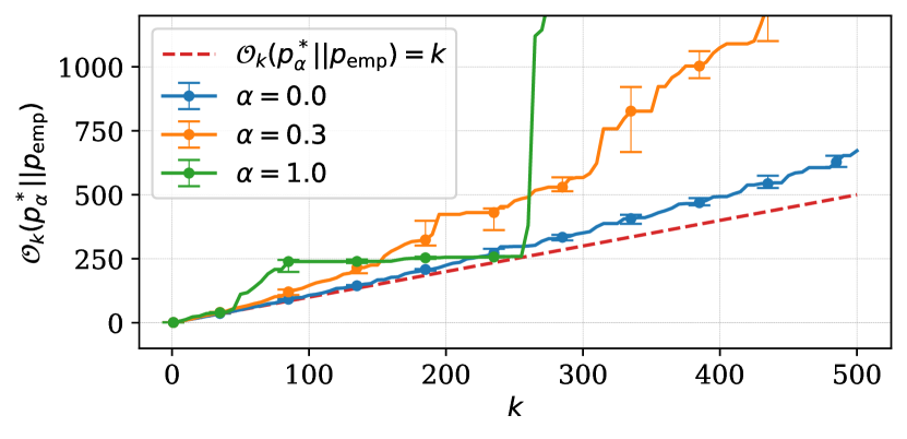
We start by asking: does mode degradation happen during data collection? We fix $N_{\text{train}}=5\times 10^{5}$ and compute mode recovery cost from the ground-truth distribution with the empirical distribution for the range of $k\leq 500$ presented in fig. 1 using three configurations of ground-truth distributions. It shows that mode recovery cost grows as $k$ increases. Furthermore, we observe different patterns of mode recovery cost given each choice of the ground-truth distribution.

We observe distinct patterns of mode recovery with either structured ($\alpha=1.0$) and unstructured ($\alpha=0.0$) ground-truth distributions. We found that the structured ground-truth distribution assigns higher probabilities to shorter sequences because of LSTM neural network and autoregressive factorization. This implies that sequences which are sorted w.r.t. their probabilities are also sorted w.r.t. their lengths. Because of this property the empirical distribution can recover modes from the structured ground-truth distribution almost perfectly for particular $k$. In the case of the unstructured ground-truth distribution mode recovery cost is lower compared to other cases. This ground-truth distribution has no statistical dependencies within modes which makes it less interesting to us due to the lack of similarity with real data.

Finally, in the case of the semi-structured ground-truth distribution ($\alpha=0.3$) the cost of recovering its modes grows increasingly as $k$ increases. In other words, empirical distributions recover modes from ground-truth distributions less effectively when latter exhibit statistical dependencies as well as many exceptional sequence probabilities.

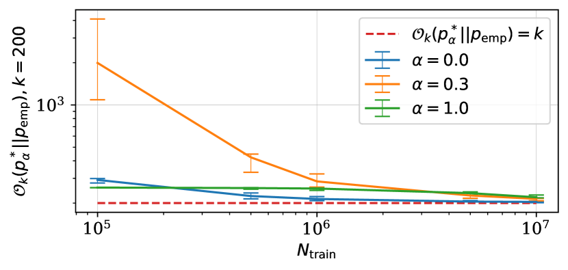
Now we focus on the influence of the training set size $N_{\text{train}}$ on mode recovery during data collection. We fix $k=200$ and compute mode recovery cost from the ground-truth distribution using the empirical distribution when $N_{\text{train}}\in\{10^{5},5\times 10^{5},10^{6},5\times 10^{6},10^{7}\}$, shown in fig. 2. Mode recovery cost naturally decreases as we increase the number of training instances as seen on the right-most side of fig. 2. The left-most side is more interesting to us because it corresponds to values of $N_{\text{train}}$ that reflect real world problems. For instance, in the case of $N_{\text{train}}=10^{5}$ it is significantly more costly to recover modes from the semi-structured ground-truth distribution compared to both structured and unstructured variants. We thus conclude that mode recovery degradation happens already during data collection, and that parameterization of ground-truth distributions impacts mode recovery cost.

The next stage in the chain is learning, $~{}p_{\mathrm{emp}}{\succ}_{\text{learning}}~{}~{}p_{\mathrm{model}}$, in which we train a model using a training dataset with the expectation that the model will match the ground-truth distribution. Our experiments center on the question: how does mode recovery degradation in the learning stage compare to that of the data collection stage? For instance, we anticipate that the learned model will have a mode recovery cost that is at least as bad as that of the empirical distribution.

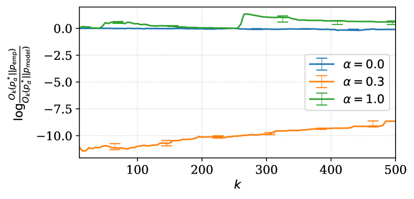
We measure the mode recovery cost reduction log-rate from empirical to learned distributions, ${\log\frac{\mathcal{O}_{k}(p^{*}_{\alpha}\|p_{\text{emp}})}{\mathcal{O}_{k}(p^{*}_{\alpha}\|p_{\text{model}})}}$. fig. 3 shows the reduction log-rate as a function of $k$ with fixed $N_{\text{train}}=5\times 10^{5}$, for three different ground-truth distributions. We observe three different cases, with a clear dependency on what kind of data was used during learning.

Learning with data coming from the unstructured ground-truth distribution ($\alpha=0.0$) results in mode recovery cost reduction log-rate being close to zero. This implies that the underlying LSTM model is able to memorize the unstructured data points coming from the empirical distribution, but it can not recover any other modes from the ground-truth distribution.

With the structured ground-truth distribution ($\alpha=1.0$), we observe positive log-rate for some values of $k$. This means that the learned distribution is able to recover modes of the ground-truth distribution at a lower cost than the empirical distribution does. Similarly to data collection stage, this largely happens due to the property of LSTM to put high probabilities on short sequences. The learned distribution’s ability in mode recovery goes above that of the empirical distribution when there is a match between the parameterization of models behind the ground-truth distribution and the learned distribution.

In the case of the semi-structured ground-truth distribution ($\alpha=0.3$), the learned distribution has severe mode recovery degradation even with smaller values of $k$ (left-most side of fig. 3). The model is unable to perfectly learn an underlying dataset which has a few statistical exceptions within it.

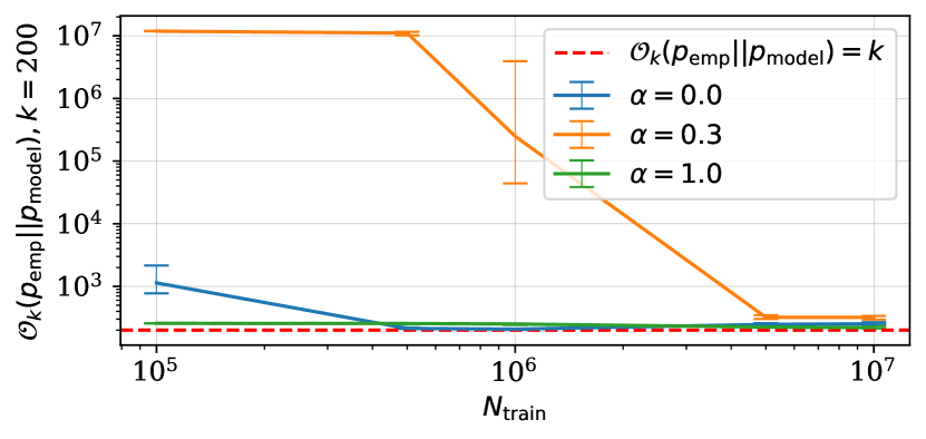
In addition to our observations about recovering modes from ground-truth distributions, fig. 4 shows at what cost modes of each empirical distribution are recovered by the learned distribution as a function of $N_{\text{train}}$. The learned distribution recovers modes of the empirical distribution with the highest cost when the latter was induced using the semi-structured ground-truth distribution. Mode recovery cost of all empirical distributions naturally decreases as number of training instances $N_{\text{train}}$ becomes unrealistically high. We conjecture that the combination of sequences with statistical dependencies and sequences which do not share any statistical dependencies in the dataset makes the learned distribution struggling at mode recovery from both ground-truth and empirical distributions.

We conclude that properties of ground-truth distributions have direct impacts on the ability of the learned distributions to recover modes from ground-truth and empirical distributions. Learning struggles to capture all patterns from the underlying distributions when the latter exhibit exceptions in statistical dependencies within data points.

The final stage in the learning chain is decoding, $p_{\mathrm{model}}{\succ}_{\text{decoding}}~{}~{}p_{\mathcal{F}}$, in which we use a decoding algorithm $\mathcal{F}$ to obtain highly-probable sequences. We study both a deterministic decoding algorithm, implemented using beam search, and a stochastic decoding algorithm, implemented using ancestral sampling. Our experiments are centered on two questions: (1) how do the choices made earlier in the learning chain affect the decoding behavior? and (2) how is this behavior affected by the choice of the decoding algorithm?

We consider six different datasets that we train models on, each of which is a combination of the ground-truth distribution where $\alpha\in\{0.0,0.3,1.0\}$, and the number of training points $N_{\text{train}}\in\{5\times 10^{5},5\times 10^{6}\}$. Our previous analysis revealed each of those datasets leads to a substantially different ability of the learned distributions to recover modes from earlier distributions along the learning chain. We set $N_{\text{model hs}}$ to be equal to $512$. Our choice of decoding algorithms results in decoding-induced distributions with a limited support. Hence the induced distribution $p_{\mathcal{F}}$ often fails to recover modes of distributions from the earlier stage of the chain especially as $k$ increases. As we described in Section 3, we use the $k$-mode set overlap $\mathcal{I}_{k}(\cdot\|p_{\mathcal{F}})$ to examine the degree to which a given decoding algorithm $\mathcal{F}$ fails at mode recovery.

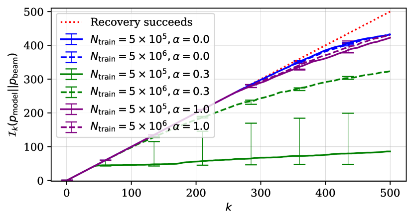
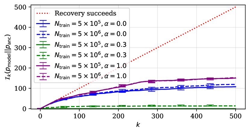
First, we study how well the decoding algorithm recovers modes from the learned distribution. fig. 5 shows $k$-mode set overlap between learned and decoding-induced distributions using both beam search (left) and ancestral sampling (right). Both algorithms fail increasingly more often as $k$ increases. Ancestral sampling fails substantially more often than beam search. This is expected given that ancestral sampling was not designed to find highly probable sequences, unlike beam search. Both of these decoding algorithms fail to recover modes from the learned distribution most when the learned distribution was obtained using the semi-structured ground-truth distribution ($\alpha=0.3$), regardless of the size of the dataset. In other words, the choices made earlier along the learning chain impact the decoding-induced distribution’s ability to recover modes from the learned distribution, regardless of which decoding algorithm was used.

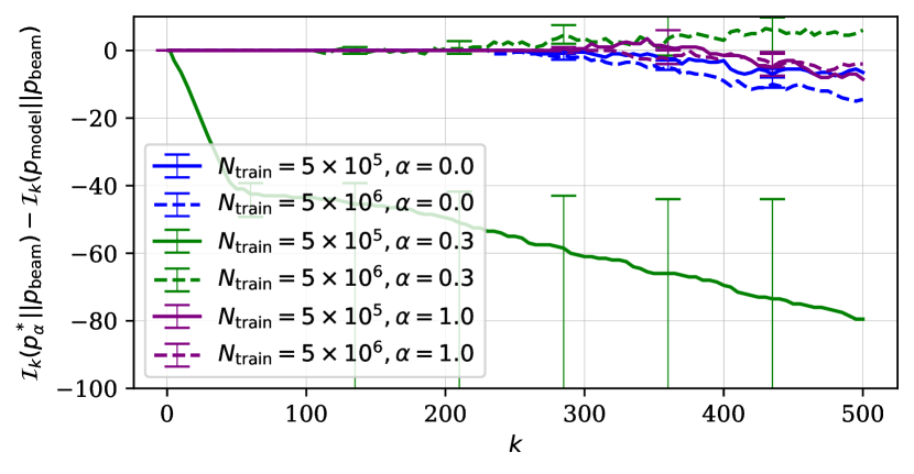
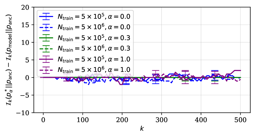
Second, we investigate how the choice of the decoding algorithm influences the difference in how the decoding-induced distribution recovers modes of ground-truth and learned distributions. We thus look at the $k$-mode set overlap reduction from ground-truth to learned distributions ($\mathcal{I}_{k}(p^{*}_{\alpha}\|p_{\mathcal{F}})-\mathcal{I}_{k}(p_{\text{model}}\|p_{\mathcal{F}})$) for both beam search and ancestral sampling. The positive overlap reduction in fig. 6 means that the decoding algorithm fails more to recover modes from the learned distribution than from the ground-truth distribution.

Each decoding algorithm shows a different pattern of the overlap reduction. Reduction is more or less flat and is close to zero for ancestral sampling regardless of the choice of the dataset. It is, however, different with beam search where we have three observations. First, the reduction overlap deviates from zero as $k$ increases. Second, with the semi-structured ground-truth distribution ($\alpha=0.3$) the overlap deviates most, which is then followed by the unstructured variant ($\alpha=0.0$). Third, the number of training points $N_{\text{train}}$ leads to significant difference in the case of the semi-structured distribution. Reduction overlap goes very negative with the smaller number of training instances, while the trend flips when we have ten times more data. We thereby conclude that the pattern of mode recovery degradation along the entire learning chain depends on the choice of the decoding algorithm.

We highlight three main directions of research based on our findings and conclusions. First, mode recovery along the learning chain must be studied in the context of real world problems. To do so, there is a need for future work on approximation schemes of mode recovery cost computable in real tasks. Second, the relationship between the ground-truth and learned distributions may be changed to better match real-world cases, for instance by considering structured ground-truth distributions that are less similar to the learned model family, or unstructured components that are informed by sequence content. Third, we have considered standard practices of neural autoregressive modeling while constructing the learning chain. Extending the learning chain to study the effects of new approaches such as knowledge distillation (Kim and Rush, 2016) or back translation (Sennrich et al., 2016) is another fruitful direction for future research.

References

- Aharoni et al. (2019) Roee Aharoni, Melvin Johnson, and Orhan Firat. 2019. Massively multilingual neural machine translation. arXiv preprint arXiv:1903.00089.
- Andor et al. (2016) Daniel Andor, Chris Alberti, David Weiss, Aliaksei Severyn, Alessandro Presta, Kuzman Ganchev, Slav Petrov, and Michael Collins. 2016. Globally normalized transition-based neural networks. In 54th Annual Meeting of the Association for Computational Linguistics, ACL 2016 - Long Papers.
- Basu et al. (2021) Sourya Basu, Govardana Sachitanandam Ramachandran, Nitish Shirish Keskar, and Lav R. Varshney. 2021. Mirostat: A neural text decoding algorithm that directly controls perplexity. In International Conference on Learning Representations.
- Brown et al. (2020) Tom B Brown, Benjamin Mann, Nick Ryder, Melanie Subbiah, Jared Kaplan, Prafulla Dhariwal, Arvind Neelakantan, Pranav Shyam, Girish Sastry, Amanda Askell, et al. 2020. Language models are few-shot learners. arXiv preprint arXiv:2005.14165.
- Deng et al. (2020) Yuntian Deng, Anton Bakhtin, Myle Ott, Arthur Szlam, and Marc’Aurelio Ranzato. 2020. Residual energy-based models for text generation. In International Conference on Learning Representations.
- Eikema and Aziz (2020) Bryan Eikema and Wilker Aziz. 2020. Is MAP decoding all you need? the inadequacy of the mode in neural machine translation. In Proceedings of the 28th International Conference on Computational Linguistics, pages 4506–4520, Barcelona, Spain (Online). International Committee on Computational Linguistics.
- Hochreiter and Schmidhuber (1997) S. Hochreiter and J. Schmidhuber. 1997. Long short-term memory. Neural Computation, 9:1735–1780.
- Holtzman et al. (2019) Ari Holtzman, Jan Buys, Li Du, Maxwell Forbes, and Yejin Choi. 2019. The curious case of neural text degeneration. arXiv preprint arXiv:1904.09751.
- Kim and Rush (2016) Yoon Kim and Alexander M. Rush. 2016. Sequence-level knowledge distillation. Proceedings of the 2016 Conference on Empirical Methods in Natural Language Processing.
- Kingma and Ba (2014) Diederik P Kingma and Jimmy Ba. 2014. Adam: A method for stochastic optimization. arXiv preprint arXiv:1412.6980.
- Lee et al. (2018) Katherine Lee, Orhan Firat, Ashish Agarwal, Clara Fannjiang, and David Sussillo. 2018. Hallucinations in neural machine translation.
- Martins et al. (2020) Pedro Henrique Martins, Zita Marinho, and André F. T. Martins. 2020. Sparse text generation. In Proceedings of the 2020 Conference on Empirical Methods in Natural Language Processing (EMNLP), pages 4252–4273, Online. Association for Computational Linguistics.
- Merity et al. (2016) Stephen Merity, Caiming Xiong, James Bradbury, and Richard Socher. 2016. Pointer sentinel mixture models.
- Murray and Chiang (2018) Kenton Murray and David Chiang. 2018. Correcting length bias in neural machine translation. In Proceedings of the Third Conference on Machine Translation: Research Papers, pages 212–223, Brussels, Belgium. Association for Computational Linguistics.
- Roller et al. (2020) Stephen Roller, Emily Dinan, Naman Goyal, Da Ju, Mary Williamson, Yinhan Liu, Jing Xu, Myle Ott, Kurt Shuster, Eric M Smith, et al. 2020. Recipes for building an open-domain chatbot. arXiv preprint arXiv:2004.13637.
- Sennrich et al. (2016) Rico Sennrich, Barry Haddow, and Alexandra Birch. 2016. Improving neural machine translation models with monolingual data. Proceedings of the 54th Annual Meeting of the Association for Computational Linguistics (Volume 1: Long Papers).
- Shi et al. (2020) Xing Shi, Yijun Xiao, and Kevin Knight. 2020. Why neural machine translation prefers empty outputs.
- Sountsov and Sarawagi (2016) Pavel Sountsov and Sunita Sarawagi. 2016. Length bias in encoder decoder models and a case for global conditioning. In EMNLP 2016 - Conference on Empirical Methods in Natural Language Processing, Proceedings.
- Stahlberg and Byrne (2019) Felix Stahlberg and Bill Byrne. 2019. On NMT search errors and model errors: Cat got your tongue? In Proceedings of the 2019 Conference on Empirical Methods in Natural Language Processing and the 9th International Joint Conference on Natural Language Processing (EMNLP-IJCNLP), pages 3354–3360, Hong Kong, China. Association for Computational Linguistics.
- Vaswani et al. (2017) Ashish Vaswani, Noam Shazeer, Niki Parmar, Jakob Uszkoreit, Llion Jones, Aidan N Gomez, Lukasz Kaiser, and Illia Polosukhin. 2017. Attention is all you need. arXiv preprint arXiv:1706.03762.
- Welleck and Cho (2020) Sean Welleck and Kyunghyun Cho. 2020. Mle-guided parameter search for task loss minimization in neural sequence modeling.
- Welleck et al. (2020a) Sean Welleck, Ilia Kulikov, Jaedeok Kim, Richard Yuanzhe Pang, and Kyunghyun Cho. 2020a. Consistency of a recurrent language model with respect to incomplete decoding. arXiv preprint arXiv:2002.02492.
- Welleck et al. (2020b) Sean Welleck, Ilia Kulikov, Stephen Roller, Emily Dinan, Kyunghyun Cho, and Jason Weston. 2020b. Neural text generation with unlikelihood training. In International Conference on Learning Representations.