\xpatchcmd

\thm@headsep
5plusminus\@begintheorem[]\xpatchcmd\cref@thmnoarg

Model Ambiguity in Risk Sharing with Monotone Mean-Variance

Emma Kroell Department of Statistical Sciences, University of Toronto emma.kroell@mail.utoronto.ca Sebastian Jaimungal Department of Statistical Sciences, University of Toronto sebastian.jaimungal@utoronto.ca Silvana M. Pesenti Department of Statistical Sciences, University of Toronto silvana.pesenti@utoronto.ca

(August 8, 2025)

Abstract

We consider the problem of an agent who faces losses over a finite time horizon and may choose to share some of these losses with a counterparty. The agent is uncertain about the true loss distribution and has multiple models for the losses. Their goal is to optimize a mean-variance type criterion with model ambiguity through risk sharing. We construct such a criterion by adapting the monotone mean-variance preferences of Maccheroni et al. (2009) to the multiple models setting and exploit a dual representation to mitigate time-consistency issues. Assuming a Cramér-Lundberg loss model, we fully characterize the optimal risk sharing contract and the agent’s wealth process under the optimal strategy. Furthermore, we prove that the strategy we obtain is admissible and prove that the value function satisfies the appropriate verification conditions. Finally, we apply the optimal strategy to an insurance setting using data from a Spanish automobile insurance portfolio, where we obtain differing models using cross-validation and provide numerical illustrations of the results.

Keywords— risk sharing, model ambiguity, monotone mean-variance, optimal contracting, model averaging

1 Introduction

In many applications in insurance and finance, actors may have multiple, competing models for an uncertain outcome. Reasons for this could include the need to incorporate expert opinions or the availability of multiple data sources. For example, consider an insurance company who has a model based on past claims, and who knows these claims will not be fully representative of future claims due to climate change. They could incorporate the threat of climate change by including additional models representing adverse climate change scenarios. Another example is a company moving into a new area of business, where they might need to include multiple sources of available data in their decision-making.

Our focus in this paper is on a type of model ambiguity inspired by this idea of different scenarios. We assume that there are multiple reference models, and that the agent does not know which reference models are correct. They must make a decision optimally accounting for ambiguity about these models, and therefore incorporate all models jointly into a single model penalization problem. In particular, we study the problem of an insurance company who faces insurance losses over a finite time horizon. The insurance company can share their risk with another agent, called the counterparty. The insurer then determines the optimal risk sharing strategy accounting for the multiple models and ambiguity about them.

This work differs from traditional approaches to model uncertainty or robustness in insurance and finance. Traditionally, one specifies a single reference model and searches for the worst-case outcome among alternate models, whose distance from the reference measure may be penalized using a divergence or distance measure. Commonly used divergence measures include the Kullback-Leibler divergence (relative entropy) and the Wasserstein distance. Some seminal contributions among many include [10] in economics, [21] and [23] in mathematical finance, [2] who quantify the divergence using optimal transport, and [3] for applications in actuarial science.

Model ambiguity with multiple reference models is studied by [13] in an optimal reinsurance context, where they determine the optimal reinsurance premium charged by a reinsurer with multiple models and multiple reinsurance clients. [12] study a related problem of combining multiple diffusion models and show that the optimal model is closely related to the barycentre model. Both these works penalize model ambiguity using the Kullback-Leibler divergence. In this paper, we instead use the chi-squared divergence, which is defined as follows from a probability measure ${\mathbb{Q}}$ to a probability measure ${\mathbb{P}}$ :

\chi^{2}({\mathbb{Q}}\,\|\,{\mathbb{P}}):={\mathbb{E}}^{\mathbb{P}}\left[\left(\frac{d{\mathbb{Q}}}{d{\mathbb{P}}}\right)^{2}-1\right]\,,

where $\frac{d{\mathbb{Q}}}{d{\mathbb{P}}}$ denotes the Radon-Nikodym (RN) derivative of ${\mathbb{Q}}$ with respect to ${\mathbb{P}}$ . For an overview of probability metrics including the chi-squared divergence, see [9].

Penalizing model ambiguity using chi-squared divergence is of particular interest due to its close relationship with another popular optimization criterion: the monotone mean-variance (MMV) preferences of [19, 20]. MMV preferences were introduced as the minimal monotone extension of the mean-variance preferences. In particular, MMV preferences agree with mean-variance preferences when mean-variance preferences are monotone, and are closest pointwise to the mean-variance preferences when they are not. Given a reference measure ${\mathbb{P}}$ , MMV preferences are defined as

\min_{{\mathbb{Q}}\in\Delta^{2}({\mathbb{P}})}\left({\mathbb{E}}^{\mathbb{Q}}[X]+\frac{1}{2\theta}\,\chi^{2}({\mathbb{Q}}\,\|\,{\mathbb{P}})\right)\,,

where $X\in{\mathcal{L}}^{2}({\mathbb{P}})$ , $\Delta^{2}({\mathbb{P}})=\{{\mathbb{Q}}\ll{\mathbb{P}}:{\mathbb{E}}^{\mathbb{P}}\left[\left(\frac{d{\mathbb{Q}}}{d{\mathbb{P}}}\right)^{2}\right]<\infty\}$ , and $\theta>0$ is a parameter penalizing uncertainty. In our work, we incorporate the chi-squared divergence between multiple reference measures ${\mathbb{P}}_{1},\ldots,{\mathbb{P}}_{n}$ and a candidate measure ${\mathbb{Q}}$ :

\min_{{\mathbb{Q}}\in\Delta^{2}}\left({\mathbb{E}}^{\mathbb{Q}}[X]+\frac{1}{2\theta}\sum_{k=1}^{n}\pi_{k}\,\chi^{2}({\mathbb{Q}}\,\|\,{\mathbb{P}}_{k})\right)\,,

(1)

where $0\leq\pi_{k}\leq 1$ are weights such that $\sum_{k=1}^{n}\pi_{k}=1$ and $\Delta^{2}:=\bigg{\{}{\mathbb{Q}}:{\mathbb{Q}}\ll{\mathbb{P}}_{k}\text{ and }{\mathbb{E}}^{{\mathbb{P}}_{k}}\left[\left(\tfrac{d{\mathbb{Q}}}{d{\mathbb{P}}_{k}}\right)^{2}\right]<\infty\,\allowbreak\text{ for all }k=1,\ldots,n\bigg{\}}$ . With this criterion, we generalize both works on model ambiguity with multiple models by using a different divergence function, and works on MMV by incorporating multiple models.

Given the connection between our model ambiguity problem and monotone mean-variance preferences, we mention here some important works that use this criterion. In recent years, there has been interest in applying MMV preferences to optimal investment problems. Examples include [30], who study an investment problem in an incomplete market and [27] and [11] who study the problem with trading constraints. The general finding has been that the optimal strategies of MMV and classical mean-variance coincide, and this is proved by [29] and [8] in general settings, under the assumption of continuous asset prices. Recently, [18] showed that MMV and traditional mean-variance preferences coincide in a Lévy market under a specific market assumption. There has also been recent interest in applying MMV to problems in optimal insurance; see [15, 17, 28, 16] for examples in both the diffusive and jump process settings.

While we incorporate model ambiguity into a mean-variance problem through a chi-squared penalization, another approach in the literature instead incorporates model ambiguity into a Nash subgame-perfect equilibrium problem. These problems assure a time-consistent approach to the mean-variance problem by searching for an intrapersonal equilibrium point (see [1] for an overview of this approach). [32] use this perspective to find the robust reinsurance and investment strategies of an insurer. [31] expand it to a Stackelberg game between an insurance company and a reinsurance company, and find that model ambiguity increases the price of reinsurance. [6] use this approach to study a risk sharing problem with $n$ insurers, and show that the Pareto optimal risk sharing strategy is a combination of a proportional and an excess-of-loss reinsurance strategy.

This work has several contributions. Using the model ambiguity criterion given by (1), we study a broad risk sharing problem, where the insurer may share any functional of its risk with a counterparty. We solve this problem and obtain closed-form expressions for the optimal strategies and the insurer’s wealth process. The key to the approach is the introduction of auxiliary processes, which represent the Radon-Nikodym derivative between each reference model and the optimal model. Furthermore, we derive an explicit expression for the insurer’s wealth process under the optimal strategy in terms of the auxiliary processes and find that the optimal wealth process is linear in the auxiliary processes. Using this result, we derive many properties of the optimal strategy, including its mean and variance. We find that the model penalization parameter acts to penalize the variance of the insurer’s wealth process. We also show how our work contains the monotone mean-variance preferences as a special case, and determine the optimal strategy in this case. Finally, we explore how the counterparty could determine the optimal premium to charge for the risk-sharing contract, showing when they wish to enter such a contract.

The rest of the paper is structured as follows. Section 2 establishes the problem setting and requisite mathematical preliminaries. In Section 3, we state our optimization problem and solve for the insurer’s optimal risk sharing strategy, as well as the optimal decision measure, ${\mathbb{Q}}^{*}$ . We further develop semi-explicit formulas for the key processes, derive their properties under the ${\mathbb{Q}}^{*}$ -measure, and provide a verification theorem. In Section 4, we apply our results to the simpler case where there is only one reference model, in which case our criterion reduces to the MMV criterion. In Section 5, we consider the pricing of such risk sharing contracts and determine how the counterparty could set the price. Finally, in Section 6, we apply our results to an example using data from a Spanish auto insurer, and illustrate the solution numerically.

2 Problem setting

Let $(\Omega,{\mathcal{F}},\mathbb{F}=({\mathcal{F}}_{t})_{t\in[0,T]})$ be a completed and filtered measurable space. Let ${\mathbb{P}}_{1},\ldots,{\mathbb{P}}_{n},{\mathbb{P}}_{C}$ be $n+1$ equivalent probability measures defined on $(\Omega,{\mathcal{F}},\mathbb{F})$ and let $\mathcal{I}:=\{1,\ldots,n,C\}$ — the element $C$ denotes the index of the counterparty while the elements $1,\dots,n$ denote the index of individual models.

Denote by $N(d\xi,dt)$ a Poisson random measure (PRM), which drives the insurance losses in the market. We assume that under a measure ${\mathbb{P}}_{k}$ for $k\in{\mathcal{I}}$ , $N$ has ${\mathbb{P}}_{k}$ -compensator $\nu_{k}(d\xi,dt)=\nu_{k}(d\xi)dt$ and define the ${\mathbb{P}}_{k}$ -compensated PRM by

\tilde{N}^{{\mathbb{P}}_{k}}(d\xi,dt)=N(d\xi,dt)-\nu_{k}(d\xi)dt\,.

We assume that each compensator admits a density denoted by $v_{k}(\xi)$ , i.e., $\nu_{k}(d\xi)=v_{k}(\xi)d\xi$ for $k\in{\mathcal{I}}$ , that has essential support on ${\mathds{R}}_{+}$ . Furthermore, we assume that for all $k\in{\mathcal{I}}$

\int_{{\mathds{R}}_{+}}\!\!\!\nu_{k}(d\xi)<\infty\quad\text{and}\quad\int_{{\mathds{R}}_{+}}\!\!\!\xi\,\nu_{k}(d\xi)<\infty\,,

and that

\int_{{\mathds{R}}_{+}}\!\!\!\xi^{2}\,\nu_{C}(d\xi)<\infty\,.

Next, we make two technical assumptions about the integrability of the compensators, which are required to assure the existence of the optimal risk sharing strategy. Essentially, these assumptions imply that the models for the loss distribution are not vastly different.

Assumption 2.1.

For all $k\in{\mathcal{I}}$

\int_{{\mathds{R}}_{+}}\frac{v_{C}^{2}(\xi)}{v_{k}(\xi)}\,d\xi<\infty\,.

For example, if we assume that $\nu_{k}(d\xi)$ is compound Poisson such that $v_{k}(\xi)=\lambda_{k}f_{k}(\xi)$ , where $\lambda_{k}>0$ and $f_{k}$ is the density of a Gamma distribution with shape $m_{k}>0$ and scale $\phi_{k}>0$ , 2.1 is satisfied if $2m_{C}>m_{k}$ and $2\phi_{k}>\phi_{C}$ for all $k\in{\mathcal{I}}\setminus\{C\}$ .

Assumption 2.2.

For all $j,k\in{\mathcal{I}}$

\int_{{\mathds{R}}_{+}}\frac{v_{C}^{3}(\xi)}{v_{j}(\xi)v_{k}(\xi)}\,d\xi<\infty\,.

Continuing the same example with a Gamma severity distribution, 2.2 is satisfied if for all $j,k\in{\mathcal{I}}\setminus\{C\}$ , $3m_{C}>m_{j}+m_{k}$ and $3\phi_{j}\phi_{k}>\phi_{C}(\phi_{j}+\phi_{k})$ .

2.1 Insurer’s wealth process

Our focus is on the behaviour of an insurance company who faces an insurable loss and receives premium income to compensate for this. The insurer charges a constant premium rate $c>0$ . Initially, the insurer’s wealth process follows the Cramér-Lundberg model:

X_{t}^{CL}=x+c\,t-\int_{0}^{t}\!\!\int_{{\mathds{R}}_{+}}\!\!\!\xi\,N(d\xi,ds)\,,

(2)

where $x>0$ is the insurer’s initial wealth.

The insurer can share their risk with another agent, who we refer to as the counterparty. They could be another insurance company, a reinsurer, or another financial entity. The insurer shares a functional $\alpha_{t}(\xi)$ of the loss $\xi\in{\mathds{R}}_{+}$ with the counterparty. The counterparty accepts the risk sharing $\alpha_{t}(\xi)$ and in turn charges a premium based on the amount of risk shared. We assume that the counterparty charges the expected value premium principle calculated under their own model, which is given by the probability measure ${\mathbb{P}}_{C}$ . They markup the expected ceded loss by a markup rate $\eta>0$ , also called the safety loading in an insurance setting. Thus the risk sharing premium is $p_{C}=(1+\eta)\int_{{\mathds{R}}_{+}}\alpha_{t}(\xi)\nu_{C}(d\xi)$ . We assume that the risk sharing premium is set such that $c<(1+\eta)\int_{{\mathds{R}}_{+}}\xi\,\nu_{C}(d\xi)$ , i.e. passing the full risk to the counterparty is not optimal.

Definition 2.3 (Admissible risk sharing strategies).

We define the set of admissible risk sharing strategies, ${\mathcal{A}}$ , as those strategies $(\alpha_{t}(\cdot))_{t\in[0,T]}$ that are ${\mathbb{F}}$ -predictable random fields, $\alpha_{t}:{\mathds{R}}_{+}\to{\mathds{R}}$ , satisfying

{\mathbb{E}}^{{\mathbb{P}}_{C}}\left[\int_{0}^{T}\!\!\!\int_{{\mathds{R}}_{+}}\!\!\!|\alpha_{s}(\xi)|^{2}\,\nu_{C}(d\xi)ds\right]<\infty\quad\text{and}\quad{\mathbb{E}}^{{\mathbb{P}}_{C}}\left[\int_{0}^{T}\!\!\!\int_{{\mathds{R}}_{+}}\!\!\left[\xi-\alpha_{s}(\xi)\right]^{2}\nu_{C}(d\xi)ds\right]<\infty\,.

Given the above assumptions, the insurer’s wealth process with risk sharing evolves according to the following equation:

X_{t}^{\alpha}=x+\int_{0}^{t}\left[c-(1+\eta)\int_{{\mathds{R}}_{+}}\!\!\!\alpha_{s}(\xi)\,\nu_{C}(d\xi)\right]ds-\int_{0}^{t}\!\!\int_{{\mathds{R}}_{+}}\!\!\![\xi-\alpha_{s}(\xi)]\,N(d\xi,ds)\,.

(3)

2.2 Insurer’s criterion

In this section, we introduce the insurer’s criterion. The insurer is uncertain about the correct model for the insurable loss. They have access to $n+1$ models for the insurable loss, given by the probability measures ${\mathbb{P}}_{k}$ for $k\in{\mathcal{I}}$ , which correspond to the counterparty’s model ${\mathbb{P}}_{C}$ and the $n$ other models ${\mathbb{P}}_{1},\ldots,{\mathbb{P}}_{n}$ . The insurer has varying degrees of certainty about the models, and may disregard some of them completely. Their goal is to determine the optimal way to share their risk with the counterparty, taking into account this uncertainty about the true loss distribution.

Our criterion is inspired by the monotone mean-variance criterion of [19, 20]. We begin by recalling this criterion, which is stated in terms of a single reference model ${\mathbb{P}}$ :

\min_{{\mathbb{Q}}\in\Delta^{2}({\mathbb{P}})}\left({\mathbb{E}}^{\mathbb{Q}}[X^{\alpha}_{T}]+\frac{1}{2\theta}{\mathbb{E}}^{\mathbb{P}}\left[\left(\frac{d{\mathbb{Q}}}{d{\mathbb{P}}}\right)^{2}-1\right]\right)\,,

where $\Delta^{2}({\mathbb{P}})=\Big{\{}{\mathbb{Q}}\ll{\mathbb{P}}:{\mathbb{E}}^{\mathbb{P}}\left[\left(\frac{d{\mathbb{Q}}}{d{\mathbb{P}}}\right)^{2}\right]<\infty\Big{\}}$ and $\theta>0$ is a parameter penalizing uncertainty.

To incorporate the uncertainty around the $n+1$ models ${\mathbb{P}}_{k}$ , $k\in{\mathcal{I}}$ , we propose the following criterion:

Definition 2.4 (Monotone Mean-Variance Criterion with Model Ambiguity).

\min_{{\mathbb{Q}}\in\Delta^{2}}{\mathbb{E}}^{\mathbb{Q}}\left[X^{\alpha}_{T}\right]+\frac{1}{2\theta}\sum_{k\in{\mathcal{I}}}\pi_{k}\,{\mathbb{E}}^{\mathbb{P}}\left[\left(\frac{d{\mathbb{Q}}}{d{\mathbb{P}}_{k}}\right)^{2}-1\right]\,,

(4)

where $0\leq\pi_{k}\leq 1$ are weights such that $\sum_{k\in{\mathcal{I}}}\pi_{k}=1$ and

\Delta^{2}:=\left\{{\mathbb{Q}}:{\mathbb{Q}}\ll{\mathbb{P}}_{k}\text{ and }{\mathbb{E}}^{{\mathbb{P}}_{k}}\left[\left(\tfrac{d{\mathbb{Q}}}{d{\mathbb{P}}_{k}}\right)^{2}\right]<\infty\,\text{ for all }k\in{\mathcal{I}}\right\}\,.

Any of the models ${\mathbb{P}}_{k}$ , $k\in{\mathcal{I}}$ , may be excluded from the insurer’s criterion by setting $\pi_{k}=0$ for that model.

It often is convenient to express this criterion entirely under the measure ${\mathbb{Q}}$ by rewriting (4) as

\min_{{\mathbb{Q}}\in\Delta^{2}}{\mathbb{E}}^{\mathbb{Q}}\left[X^{\alpha}_{T}+\frac{1}{2\theta}\sum_{k\in{\mathcal{I}}}\pi_{k}\left(\frac{d{\mathbb{Q}}}{d{\mathbb{P}}_{k}}-1\right)\right]\,.

Next, we obtain an alternate representation of (4) by recasting the problem as a zero-sum stochastic game (see [22]). To do so, we introduce a family of stochastic processes $\{Z^{\beta}_{k,t}\}_{k\in{\mathcal{I}},t\in[0,T]}$ , which we call auxiliary processes. These processes are driven by a random field $\beta$ which we call the compensator.

Definition 2.5.

Define $\mathcal{B}$ to be the set of ${\mathbb{F}}$ -predictable random fields $(\beta_{t}(\cdot))_{t\in[0,T]}$ , $\beta_{t}:{\mathds{R}}_{+}\to{\mathds{R}}_{+}$ , satisfying for all $k\in{\mathcal{I}}$

{\mathbb{E}}^{{\mathbb{P}}_{k}}\left[\int_{0}^{T}\!\!\!\int_{{\mathds{R}}_{+}}\!\!\left[1-\frac{\beta_{s}(\xi)}{v_{k}(\xi)}\right]^{2}\!\!\nu_{k}(d\xi)ds\right]<\infty\,.

Next, for $\beta\in\mathcal{B}$ , define the stochastic processes $\left\{Z^{\beta}_{k,t}\right\}_{k\in{\mathcal{I}},t\in[0,T]}$ as follows:

dZ_{k,t}^{\beta}=-Z_{k,t^{-}}^{\beta}\int_{{\mathds{R}}_{+}}\!\!\left[1-\frac{\beta_{t}(\xi)}{v_{k}(\xi)}\right]\tilde{N}^{{\mathbb{P}}_{k}}(d\xi,dt)\,,\quad Z^{\beta}_{k,0}=1\,,\quad\text{for all }k\in{\mathcal{I}}\,.

(5)

We restrict our attention to measures ${\mathbb{Q}}_{\beta}\in\Delta^{2}$ such that $d{\mathbb{Q}}_{\beta}(\omega)=Z^{\beta}_{k,T}\,d{\mathbb{P}}_{k}(\omega)$ on ${\mathcal{F}}_{T}$ for some $\beta\in{\mathcal{B}}$ and all $k\in{\mathcal{I}}$ .

Definition 2.6 (Admissible compensators).

Let ${\mathfrak{B}}$ denote the ${\mathbb{F}}$ -predictable random fields $\beta\in\mathcal{B}$ such that, for all $k\in{\mathcal{I}}$ ,

{\mathbb{E}}^{{\mathbb{P}}_{k}}\left[Z_{k,T}^{\beta}\right]=1\quad\text{and}\quad{\mathbb{E}}^{{\mathbb{P}}_{k}}\left[\left(Z_{k,T}^{\beta}\right)^{2}\right]<\infty\,.

Then, from Girsanov’s Theorem for random measures, under a candidate measure ${\mathbb{Q}}_{\beta}$ , for all $k\in{\mathcal{I}}$ ,

	$\displaystyle\tilde{N}^{{\mathbb{Q}}_{\beta}}(d\xi,dt)$	$\displaystyle=\tilde{N}^{{\mathbb{P}}_{k}}(d\xi,dt)+\left[1-\frac{\beta_{t}(\xi)}{v_{k}(\xi)}\right]\nu_{k}(d\xi)dt$
		$\displaystyle=N(d\xi,dt)-\beta_{t}(\xi)d\xi dt\,,$

is a martingale increment, i.e., $N$ has ${\mathbb{Q}}_{\beta}$ -compensator $\beta_{t}(\xi)\,d\xi\,dt$ .

Armed with this parametrization, in what follows we solve the modified problem

\inf_{\beta\in{\mathfrak{B}}}{\mathbb{E}}^{{\mathbb{Q}}_{\beta}}\left[X^{\alpha}_{T}+\frac{1}{2\theta}\sum_{k\in{\mathcal{I}}}\pi_{k}\left(Z^{\beta}_{k,T}-1\right)\right]\,.

3 The insurer’s optimal risk sharing strategy

In this section, we first state the insurer’s optimization problem and solve it for the insurer’s optimal risk sharing strategy, denoted $\alpha^{*}$ , and the optimal measure, denoted ${\mathbb{Q}}^{*}:={\mathbb{Q}}_{\beta^{*}}$ . We then show that under the optimal risk sharing strategy, the insurer’s wealth $X$ and the auxiliary processes $Z_{k}$ , $k\in{\mathcal{I}}$ , may be written in a semi-explicit form, and use this to determine the mean and variance of the processes at any time in $[0,T]$ . In particular, we show that there is a linear relationship between the optimal $X$ and the $Z_{k}$ ’s. Finally, we provide a verification theorem, showing the candidate controls are indeed optimal.

3.1 Optimization problem and candidate solution

Optimization Problem 3.1.

The insurer seeks the solution to the following problem:

\sup_{\alpha\in{\mathcal{A}}}\mathop{\mathrm{inf}\vphantom{\mathrm{sup}}}_{\beta\in{\mathfrak{B}}}{\mathbb{E}}^{{\mathbb{Q}}_{\beta}}\left[X^{\alpha}_{T}+\frac{1}{2\theta}\sum_{k\in{\mathcal{I}}}\pi_{k}\left(Z^{\beta}_{k,T}-1\right)\right]\,,

where


$\displaystyle dX_{t}^{\alpha}$	$\displaystyle=\left[c-(1+\eta)\int_{{\mathds{R}}_{+}}\!\!\!\alpha_{t}(\xi)\,\nu_{C}(d\xi)-\int_{{\mathds{R}}_{+}}\!\!\![\xi-\alpha_{t}(\xi)]\,\beta_{t}(\xi)\,d\xi\right]dt-\int_{{\mathds{R}}_{+}}\!\!\![\xi-\alpha_{t}(\xi)]\,\tilde{N}^{{\mathbb{Q}}_{\beta}}(d\xi,dt)\,,$	(6a)
$\displaystyle dZ_{k,t}^{\beta}$	$\displaystyle=Z_{k,t^{-}}^{\beta}\int_{{\mathds{R}}_{+}}\!\!\left[1-\frac{\beta_{t}(\xi)}{v_{k}(\xi)}\right]^{2}\nu_{k}(d\xi)dt-Z_{k,t^{-}}^{\beta}\int_{{\mathds{R}}_{+}}\!\!\left[1-\frac{\beta_{t}(\xi)}{v_{k}(\xi)}\right]\tilde{N}^{{\mathbb{Q}}_{\beta}}(d\xi,dt)\,,\qquad\forall\;k\in{\mathcal{I}},$	(6b)

with $X_{0}=x$ , $Z_{k,0}=1$ for all $k\in{\mathcal{I}}$ .

We obtain the dynamics of $X^{\alpha}$ and $Z_{k}^{\beta}$ , $k\in{\mathcal{I}}$ , given in (6) by writing the original dynamics given in (3) and (5) in terms of the candidate measure ${\mathbb{Q}}_{\beta}$ .

Let $\boldsymbol{Z}_{t}=(Z_{1,t},\ldots,Z_{n,t},Z_{C,t})$ be the vector version of the auxiliary processes and let $\boldsymbol{z}=(z_{1},\ldots,z_{n},z_{C})$ be an arbitrary vector in ${\mathds{R}}_{+}^{n+1}$ . For fixed controls $\alpha\in{\mathcal{A}}$ , $\beta\in{\mathfrak{B}}$ , we define the time- $t$ version of the value function as

J^{\alpha,\beta}(t,x,\boldsymbol{z}):={\mathbb{E}}^{{\mathbb{Q}}_{\beta}}_{t,x,\boldsymbol{z}}\left[X^{\alpha}_{T}+\frac{1}{2\theta}\sum_{k\in{\mathcal{I}}}\pi_{k}\left(Z^{\beta}_{k,T}-1\right)\right]\,,

(7)

where ${\mathbb{E}}^{{\mathbb{Q}}_{\beta}}_{t,x,\boldsymbol{z}}[\cdot]$ denotes the ${\mathbb{Q}}_{\beta}$ -expectation given that the processes $X$ , $\boldsymbol{Z}$ at time $t^{-}$ are equal to $x$ and $\boldsymbol{z}$ , respectively, i.e., $X_{t^{-}}=x$ and $\boldsymbol{Z}_{t^{-}}=\boldsymbol{z}$ . We then define the insurer’s time- $t$ optimal value function at the optimal controls as

J(t,x,\boldsymbol{z}):=\sup_{\alpha\in{\mathcal{A}}}\mathop{\mathrm{inf}\vphantom{\mathrm{sup}}}_{\beta\in{\mathfrak{B}}}J^{\alpha,\beta}(t,x,\boldsymbol{z})\,.

We first derive a candidate value function for 3.1 and the associated candidate controls. Let ${\mathfrak{S}}$ denote the set of functions $g:[0,T]\times{\mathds{R}}_{+}\times{\mathds{R}}\times{\mathds{R}}_{+}^{n+1}\to{\mathds{R}}$ such that $\int_{{\mathds{R}}_{+}}g(t,\xi,x,\boldsymbol{z})\,d\xi<\infty$ for every $t,x,\boldsymbol{z}\in[0,T]\times{\mathds{R}}\times{\mathds{R}}_{+}^{n+1}$ . The generator of the stochastic differential equations (6) for Markov controls $a,b\in{\mathfrak{S}}$ is

\displaystyle\begin{split}A^{a,b}&f(t,x,\boldsymbol{z})\\ :=&\,\partial_{t}f(t,x,\boldsymbol{z})\\ &+\left[c-(1+\eta)\int_{{\mathds{R}}_{+}}\!\!\!a(t,\xi,x,\boldsymbol{z})\,\nu_{C}(d\xi)-\int_{{\mathds{R}}_{+}}\!\!\![\xi-a(t,\xi,x,\boldsymbol{z})]\,b(t,\xi,x,\boldsymbol{z})\,d\xi\right]\partial_{x}f(t,x,\boldsymbol{z})\\ &+\sum_{k\in{\mathcal{I}}}z_{k}\int_{{\mathds{R}}_{+}}\!\!\left[1-\frac{b(t,\xi,x,\boldsymbol{z})}{v_{k}(\xi)}\right]^{2}\!\!\nu_{k}(d\xi)\,\partial_{z_{k}}f(t,x,\boldsymbol{z})\\ &+\int_{{\mathds{R}}_{+}}\Bigg{[}f\!\left(t,x-[\xi-a(t,\xi,x,\boldsymbol{z})],z_{1}\frac{b(t,\xi,x,\boldsymbol{z})}{v_{1}(\xi)},\ldots,z_{n}\frac{b(t,\xi,x,\boldsymbol{z})}{v_{n}(\xi)},z_{C}\frac{b(t,\xi,x,\boldsymbol{z})}{v_{C}(\xi)}\right)-f(t,x,\boldsymbol{z})\\ &\quad\qquad\,+[\xi-a(t,\xi,x,\boldsymbol{z})]\partial_{x}f(t,x,\boldsymbol{z})+\sum_{k\in{\mathcal{I}}}z_{k}\left(1-\frac{b(t,\xi,x,\boldsymbol{z})}{v_{k}(\xi)}\right)\partial_{z_{k}}f(t,x,\boldsymbol{z})\Bigg{]}b(t,\xi,x,\boldsymbol{z})d\xi\,,\end{split}

(8)

where $f$ is a continuously differentiable function on $(0,T)\times{\mathds{R}}\times{\mathds{R}}_{+}^{n+1}$ .

The next result states the candidate controls and value function for 3.1. We provide a verification result in Section 3.3.

Proposition 3.2.

The candidate controls for 3.1 in feedback form are


$\displaystyle\alpha^{*}(t,\xi,\boldsymbol{z})$	$\displaystyle=\xi-\frac{1}{\theta}\sum_{k\in{\mathcal{I}}}\pi_{k}\,z_{k}\,\ell_{k}(T-t)\left[(1+\eta)\frac{v_{C}(\xi)}{v_{k}(\xi)}-1\right]\,,$	(9a)
$\displaystyle\beta^{*}(\xi)$	$\displaystyle=(1+\eta)\,v_{C}(\xi)\,,$	(9b)

where

\ell_{k}(t)=\exp\left(t\int_{{\mathds{R}}_{+}}\!\!\left[1-(1+\eta)\frac{v_{C}(\xi)}{v_{k}(\xi)}\right]^{2}\!\!\nu_{k}(d\xi)\right)\,,

and the candidate value function is

J(t,x,\boldsymbol{z})=x+\frac{1}{2\theta}\sum_{k\in{\mathcal{I}}}\pi_{k}\,z_{k}\,\ell_{k}(T-t)-\frac{1}{2\theta}-\left[(1+\eta)\int_{{\mathds{R}}_{+}}\!\!\xi\,\nu_{C}(d\xi)-c\right](T-t)\,.

Before providing the proof, we first comment on the candidate optimal controls and value function. First, note that by 2.1, the integral over $\xi$ in the exponential in $\ell_{k}(t)$ is finite and thus $\ell_{k}(t)<\infty$ for all $t\in[0,T]$ . Therefore, the candidate value function is well-defined. The form of the compensator of the optimal measure, $\beta^{*}$ , is instructive: we see that the probability measure the insurer uses to determine the optimal risk sharing agreement is tied to the premium charged for the risk sharing. They use the counterparty’s model for the losses, but increase the rate of arrival multiplicatively by $1+\eta$ , where $\eta$ is the counterparty’s markup rate to the premium. The form of the optimal risk sharing strategy, $\alpha^{*}$ , is more complex. One may view it as a generalization of an excess-of-loss reinsurance contract, which is usually of the form $(\xi-d)_{+}$ for some retention limit $d>0$ . In this case, however, the “retention limit” depends on the size of the loss, $\xi$ , and there is no restriction that it be positive.

Proof.

The insurer’s value function

J(t,x,\boldsymbol{z})=\sup_{\alpha\in{\mathcal{A}}}\mathop{\mathrm{inf}\vphantom{\mathrm{sup}}}_{\beta\in{\mathfrak{B}}}{\mathbb{E}}^{{\mathbb{Q}}_{\beta}}_{t,x,\boldsymbol{z}}\left[X^{\alpha}_{T}+\frac{1}{2\theta}\sum_{k\in{\mathcal{I}}}\pi_{k}\left(Z^{\beta}_{k,T}-1\right)\right]\,,

must satisfy the Hamilton-Jacobi-Bellman-Isaacs (HJBI) equation

$\displaystyle 0$	$\displaystyle=\,\sup_{a\in{\mathfrak{S}}}\mathop{\mathrm{inf}\vphantom{\mathrm{sup}}}_{b\in{\mathfrak{S}}}\big{\{}A^{a,b}J(t,x,\boldsymbol{z})\big{\}}$	(10)
	$\displaystyle=\,\partial_{t}J(t,x,\boldsymbol{z})$
	$\displaystyle\quad+\sup_{a\in{\mathfrak{S}}}\mathop{\mathrm{inf}\vphantom{\mathrm{sup}}}_{b\in{\mathfrak{S}}}\!\!\Bigg{\{}\left[c-(1+\eta)\int_{{\mathds{R}}_{+}}\!\!\!a(t,\xi,x,\boldsymbol{z})\,\nu_{C}(d\xi)-\int_{{\mathds{R}}_{+}}\!\!\![\xi-a(t,\xi,x,\boldsymbol{z})]\,b(t,\xi,x,\boldsymbol{z})\,d\xi\right]\partial_{x}J(t,x,\boldsymbol{z})$
	$\displaystyle\hskip 65.00009pt+\sum_{k\in{\mathcal{I}}}z_{k}\int_{{\mathds{R}}_{+}}\!\!\left[1-\frac{b(t,\xi,x,\boldsymbol{z})}{v_{k}(\xi)}\right]^{2}\!\!\nu_{k}(d\xi)\,\partial_{z_{k}}J(t,x,\boldsymbol{z})$
	$\displaystyle\hskip 65.00009pt+\int_{{\mathds{R}}_{+}}\Big{[}J\!\left(t,x-[\xi-a(t,\xi,x,z)],z_{1}\frac{b(t,\xi,x,z)}{v_{1}(\xi)},\ldots,z_{n}\frac{b(t,\xi,x,z)}{v_{n}(\xi)},z_{C}\frac{b(t,\xi,x,z)}{v_{C}(\xi)}\right)$
	$\displaystyle\hskip 95.00014pt-J(t,x,\boldsymbol{z})+[\xi-a(t,\xi,x,\boldsymbol{z})]\partial_{x}J(t,x,\boldsymbol{z})$
	$\displaystyle\hskip 95.00014pt+\sum_{k\in{\mathcal{I}}}z_{k}\left[1-\frac{b(t,\xi,x,\boldsymbol{z})}{v_{k}(\xi)}\right]\partial_{z_{k}}J(t,x,\boldsymbol{z})\Big{]}b(t,\xi,x,\boldsymbol{z})d\xi\Bigg{\}}$

with terminal condition

J(T,x,\boldsymbol{z})=x+\frac{1}{2\theta}\sum_{k\in{\mathcal{I}}}\pi_{k}(z_{k}-1)\,.

(11)

Using the Ansatz

J(t,x,\boldsymbol{z})=x+\sum_{k\in{\mathcal{I}}}A_{k}(t)z_{k}+B(t)\,,

where $A_{k}$ , $k\in{\mathcal{I}}$ , and $B$ are deterministic functions satisfying $A_{k}(T)=\pi_{k}/2\theta,\,k\in{\mathcal{I}}\,,B(T)=-1/2\theta$ , we obtain the simplified HJBI equation:

\begin{split}0&=\sum_{k\in{\mathcal{I}}}A^{\prime}_{k}(t)\,z_{k}+\,B^{\prime}(t)\\ &\quad+\sup_{a\in{\mathfrak{S}}}\mathop{\mathrm{inf}\vphantom{\mathrm{sup}}}_{b\in{\mathfrak{S}}}\!\Bigg{\{}\!c-(1+\eta)\int_{{\mathds{R}}_{+}}\!\!\!a(t,\xi,x,\boldsymbol{z})\,\nu_{C}(d\xi)-\int_{{\mathds{R}}_{+}}\!\!\![\xi-a(t,\xi,x,\boldsymbol{z})]\,b(t,\xi,x,\boldsymbol{z})\,d\xi\\ &\hskip 60.00009pt+\sum_{k\in{\mathcal{I}}}z_{k}A_{k}(t)\int_{{\mathds{R}}_{+}}\!\!\left[1-\frac{b(t,\xi,x,\boldsymbol{z})}{v_{k}(\xi)}\right]^{2}\!\!\nu_{k}(d\xi)\Bigg{\}}\,.\end{split}

(12)

Next, consider the infimum problem for $b$ , where we minimize the following functional:

\mathcal{L}_{1}[b]:=\int_{{\mathds{R}}_{+}}\!\!\left(\,\sum_{k\in{\mathcal{I}}}z_{k}A_{k}(t)\!\!\left[1-\frac{b(t,\xi,x,\boldsymbol{z})}{v_{k}(\xi)}\right]^{2}\!\!v_{k}(\xi)-[\xi-a(t,\xi,x,\boldsymbol{z})]\,b(t,\xi,x,\boldsymbol{z})\right)d\xi\,.

Let $\varepsilon>0$ and $f$ be an arbitrary function such that $b+\varepsilon f\in{\mathfrak{S}}$ . We apply a variational first order condition to obtain the equation:

0=\lim_{\varepsilon\searrow 0}\frac{1}{\varepsilon}\left(\mathcal{L}[b+\varepsilon f]-\mathcal{L}[b]\right)=\int_{{\mathds{R}}_{+}}\!\!\!f(t,\xi,x,\boldsymbol{z})\left(\,2\sum_{k\in{\mathcal{I}}}z_{k}A_{k}(t)\!\!\left[\frac{b(t,\xi,x,\boldsymbol{z})}{v_{k}(\xi)}-1\right]-[\xi-a(t,\xi,x,\boldsymbol{z})]\right)d\xi\,.

As the function $f$ is arbitrary, the above expression vanishes for

\hat{b}(t,\xi,x,\boldsymbol{z})=\frac{\xi-a(t,\xi,x,\boldsymbol{z})+2\sum_{k\in{\mathcal{I}}}z_{k}A_{k}(t)}{2\sum_{k\in{\mathcal{I}}}A_{k}(t)\frac{z_{k}}{v_{k}(\xi)}}\,.

(13)

Substituting this form back into the HJBI equation (12) yields the new equation

\begin{split}0=&\,\sum_{k\in{\mathcal{I}}}A^{\prime}_{k}(t)\,z_{k}+B^{\prime}(t)+c+\sum_{k\in{\mathcal{I}}}A_{k}(t)\,z_{k}\int_{{\mathds{R}}_{+}}\!\!\!\xi\,\nu_{k}(d\xi)\\ &+\sup_{a\in{\mathfrak{S}}}\left\{-\int_{{\mathds{R}}_{+}}\!\!\left[(1+\eta)\,a(t,\xi,x,\boldsymbol{z})\,v_{C}(\xi)+\frac{\left(\xi-a(t,\xi,x,\boldsymbol{z})+2\sum_{k\in{\mathcal{I}}}z_{k}A_{k}(t)\right)^{2}}{4\sum_{k\in{\mathcal{I}}}A_{k}(t)\frac{z_{k}}{v_{k}(\xi)}}\right]d\xi\right\}\,,\end{split}

(14)

with terminal conditions $A_{k}(T)=\pi_{k}/2\theta,\,k\in{\mathcal{I}}\,,B(T)=-1/2\theta$ . Next, we solve the supremum problem for $a$ using a variational first order condition. To this end, we minimize the functional

\mathcal{L}_{2}[a]:=\int_{{\mathds{R}}_{+}}\!\!\left[(1+\eta)\,a(t,\xi,x,\boldsymbol{z})\,v_{C}(\xi)+\frac{\left(\xi-a(t,\xi,x,\boldsymbol{z})+2\sum_{k\in{\mathcal{I}}}z_{k}A_{k}(t)\right)^{2}}{4\sum_{k\in{\mathcal{I}}}A_{k}(t)\frac{z_{k}}{v_{k}(\xi)}}\right]d\xi\,.

Let $\varepsilon>0$ and $g$ be an arbitrary function such that $b+\varepsilon g\in{\mathfrak{S}}$ . Then

0=\lim_{\varepsilon\searrow 0}\frac{1}{\varepsilon}\left(\mathcal{L}_{2}[a+\varepsilon g]-\mathcal{L}_{2}[a]\right)=\int_{{\mathds{R}}_{+}}\!\!\!g(t,\xi,x,\boldsymbol{z})\left((1+\eta)\,v_{C}(\xi)-\frac{\xi-a(t,\xi,x,\boldsymbol{z})+2\sum_{k\in{\mathcal{I}}}z_{k}A_{k}(t)}{2\sum_{k\in{\mathcal{I}}}A_{k}(t)\frac{z_{k}}{v_{k}(\xi)}}\right)d\xi\,.

As $g$ is arbitrary, we obtain the following feedback form for $a$ :

\hat{a}(t,\xi,x,\boldsymbol{z})=\xi-2\sum_{k\in{\mathcal{I}}}A_{k}(t)\,z_{k}\left[(1+\eta)\frac{v_{C}(\xi)}{v_{k}(\xi)}-1\right]\,.

(15)

Substituting this expression into HBJI equation (14), we obtain

\displaystyle 0=

\displaystyle\,\sum_{k\in{\mathcal{I}}}A^{\prime}_{k}(t)\,z_{k}+B^{\prime}(t)+c-(1+\eta)\int_{{\mathds{R}}_{+}}\!\!\!\xi\,\nu_{C}(d\xi)+\sum_{k\in{\mathcal{I}}}A_{k}(t)\,z_{k}\int_{{\mathds{R}}_{+}}\!\!\left[1-(1+\eta)\frac{v_{C}(\xi)}{v_{k}(\xi)}\right]^{2}\nu_{k}(d\xi)\,

with terminal conditions $A_{k}(T)=\pi_{k}/2\theta,\,k\in{\mathcal{I}}\,,B(T)=-1/2\theta$ . Solving for the unknown functions $A_{k}(t)$ , $k\in{\mathcal{I}}$ , and $B(t)$ gives

	$\displaystyle A_{k}(t)$	$\displaystyle=\frac{\pi_{k}}{2\theta}\exp\left(\int_{{\mathds{R}}_{+}}\left[1-(1+\eta)\frac{v_{C}(\xi)}{v_{k}(\xi)}\right]^{2}\!\!\nu_{k}(d\xi)\,(T-t)\right),\quad k\in{\mathcal{I}}\,,$
	$\displaystyle B(t)$	$\displaystyle=\left[(1+\eta)\int_{{\mathds{R}}_{+}}\!\!\xi\,\nu_{C}(d\xi)-c\right](t-T)-\frac{1}{2\theta}\,.$

Substituting these functions into the Ansatz gives the insurer’s value function:

\displaystyle J(t,x,\boldsymbol{z})=

\displaystyle\,x+\frac{1}{2\theta}\sum_{k\in{\mathcal{I}}}\pi_{k}\,z_{k}\,\ell_{k}(T-t)-\frac{1}{2\theta}-\left[(1+\eta)\int_{{\mathds{R}}_{+}}\!\!\xi\,\nu_{C}(d\xi)-c\right](T-t)\,,

where

\ell_{k}(t):=\exp\left(t\int_{{\mathds{R}}_{+}}\left[1-(1+\eta)\frac{v_{C}(\xi)}{v_{k}(\xi)}\right]^{2}\!\!\nu_{k}(d\xi)\right)\,.

Furthermore, simplifying (13) and (15) and subtituting in the $A_{k}(t)$ , $k\in{\mathcal{I}}$ , gives the candidate optimal controls:

	$\displaystyle\alpha^{*}(t,\xi,\boldsymbol{z})$	$\displaystyle=\xi-\frac{1}{\theta}\sum_{k\in{\mathcal{I}}}\pi_{k}\,z_{k}\,\ell_{k}(T-t)\left[(1+\eta)\frac{v_{C}(\xi)}{v_{k}(\xi)}-1\right]\,,$
	$\displaystyle\beta^{*}(\xi)$	$\displaystyle=(1+\eta)\,v_{C}(\xi)\,.\qed$

3.2 Processes under optimal controls

Next, we derive expressions for the processes $X$ and $\boldsymbol{Z}$ under the candidate controls $\alpha^{*}$ and $\beta^{*}$ , which we denote by $X^{*}$ and $\boldsymbol{Z}^{*}$ , respectively. We find that $X^{*}$ and $\boldsymbol{Z}^{*}$ have a relatively simple form, which allows us to calculate their mean and variance. The processes under the optimal controls satisfy the SDEs:

\begin{split}dX_{t}^{*}&=\left[c-(1+\eta)\int_{{\mathds{R}}_{+}}\!\!\!\xi\,\nu_{C}(d\xi)+\frac{1+\eta}{\theta}\sum_{k\in{\mathcal{I}}}\pi_{k}Z^{*}_{k,t^{-}}\ell_{k}(T-t)\int_{{\mathds{R}}_{+}}\!\!\!\left[(1+\eta)\frac{v_{C}(\xi)}{v_{k}(\xi)}-1\right]\nu_{C}(d\xi)\right]dt\\ &\quad-\frac{1}{\theta}\sum_{k\in{\mathcal{I}}}\pi_{k}Z^{*}_{k,t^{-}}\ell_{k}(T-t)\int_{{\mathds{R}}_{+}}\!\!\!\left[(1+\eta)\frac{v_{C}(\xi)}{v_{k}(\xi)}-1\right]N(d\xi,dt)\,,\\ X_{0}^{*}&=x\,,\end{split}

where

\ell_{k}(t)=\exp\left(t\int_{{\mathds{R}}_{+}}\!\!\left[1-(1+\eta)\frac{v_{C}(\xi)}{v_{k}(\xi)}\right]^{2}\!\!\nu_{k}(d\xi)\right)\quad\text{for }k\in{\mathcal{I}}\,,

and for $k\in{\mathcal{I}}$ ,

\begin{split}dZ^{*}_{k,t}&=Z^{*}_{k,t^{-}}\int_{{\mathds{R}}_{+}}\!\!\!\left[v_{k}(\xi)-(1+\eta)v_{C}(\xi)\right]d\xi dt-Z^{*}_{k,t^{-}}\int_{{\mathds{R}}_{+}}\!\!\!\left[1-(1+\eta)\frac{v_{C}(\xi)}{v_{k}(\xi)}\right]N(d\xi,dt)\,,\\ Z^{*}_{k,0}&=1\,.\end{split}

Using Itô’s lemma, we solve these SDEs and find that $X^{*}$ may be written as a linear combination of the $Z^{*}_{k}$ ’s.

Proposition 3.3.

For $t\in[0,T]$ :

	$\displaystyle Z^{*}_{k,t}$	$\displaystyle=\exp\left(t\int_{{\mathds{R}}_{+}}\!\!\!\left[v_{k}(\xi)-(1+\eta)v_{C}(\xi)\right]d\xi+\int_{0}^{t}\!\!\int_{{\mathds{R}}_{+}}\!\!\!\ln\left((1+\eta)\frac{v_{C}(\xi)}{v_{k}(\xi)}\right)N(d\xi,ds)\right)\,,\quad k\in{\mathcal{I}}\,,$
	$\displaystyle X^{*}_{t}$	$\displaystyle=x+\left[c-(1+\eta)\int_{{\mathds{R}}_{+}}\!\!\!\xi\,\nu_{C}(d\xi)\right]t+\frac{1}{\theta}\sum_{k\in{\mathcal{I}}}\pi_{k}\,\ell_{k}(T)\,\left[1-\ell_{k}(-t)Z^{*}_{k,t}\right]\,.$

Proof.

For $Z^{*}_{k,t}$ , applying Itô’s formula for semimartingales to the function $\ln(Z^{*}_{k,t})$ for each $k\in{\mathcal{I}}$ gives

	$\displaystyle\ln(Z^{*}_{k,t})=$	$\displaystyle\,\ln(Z^{}_{k,0})+\int_{0}^{t}\frac{1}{Z^{}_{k,s^{-}}}dZ^{*}_{k,s}$
		$\displaystyle+\int_{0}^{t}\!\!\int_{{\mathds{R}}_{+}}\!\!\!\left\{\ln\left(Z^{}_{k,s^{-}}-Z^{}_{k,s^{-}}\left[1-(1+\eta)\frac{v_{C}(\xi)}{v_{k}(\xi)}\right]\right)-\ln(Z^{*}_{k,s^{-}})+\left[1-(1+\eta)\frac{v_{C}(\xi)}{v_{k}(\xi)}\right]\right\}N(d\xi,ds)$
	$\displaystyle=$	$\displaystyle\int_{0}^{t}\!\!\int_{{\mathds{R}}_{+}}\!\!\!\left[v_{k}(\xi)-(1+\eta)v_{C}(\xi)\right]d\xi ds-\int_{0}^{t}\!\!\int_{{\mathds{R}}_{+}}\!\!\!\left[1-(1+\eta)\frac{v_{C}(\xi)}{v_{k}(\xi)}\right]N(d\xi,ds)$
		$\displaystyle+\int_{0}^{t}\!\!\int_{{\mathds{R}}_{+}}\!\!\!\left\{\ln\left((1+\eta)\frac{v_{C}(\xi)}{v_{k}(\xi)}\right)+\left[1-(1+\eta)\frac{v_{C}(\xi)}{v_{k}(\xi)}\right]\right\}N(d\xi,ds)$
	$\displaystyle=$	$\displaystyle\int_{0}^{t}\!\!\int_{{\mathds{R}}_{+}}\!\!\!\left[v_{k}(\xi)-(1+\eta)v_{C}(\xi)\right]d\xi ds+\int_{0}^{t}\!\!\int_{{\mathds{R}}_{+}}\!\!\!\ln\left((1+\eta)\frac{v_{C}(\xi)}{v_{k}(\xi)}\right)N(d\xi,ds)\,.$

Exponentiation gives the result.
For $X^{*}_{t}$ , define the function

f(t,X^{*}_{t},\boldsymbol{Z}^{*}_{t})=X^{*}_{t}+\frac{1}{\theta}\sum_{k\in{\mathcal{I}}}\pi_{k}\,\ell_{k}(T-t)Z^{*}_{k,t}-\left[c-(1+\eta)\int_{{\mathds{R}}_{+}}\!\!\!\xi\,\nu_{C}(d\xi)\right]t-\frac{1}{\theta}\sum_{k\in{\mathcal{I}}}\pi_{k}\,\ell_{k}(T)\,.

Then by Itô’s formula for multi-dimensional semimartingales (see, e.g., [24, Theorem 33]), we have

	$\displaystyle f(t,X^{}_{t},\boldsymbol{Z}^{}_{t})=$	$\displaystyle\,f(0,X^{}_{0},\boldsymbol{Z}^{}_{0})+\int_{0}^{t}\frac{\partial f}{\partial s}(s,X^{}_{s^{-}},\boldsymbol{Z}^{}_{s^{-}})\,ds$
		$\displaystyle+\int_{0}^{t}\frac{\partial f}{\partial x}(s,X^{}_{s^{-}},\boldsymbol{Z}^{}_{s^{-}})dX^{}_{s}+\sum_{k\in{\mathcal{I}}}\int_{0}^{t}\frac{\partial f}{\partial z_{k}}(s,X^{}_{s^{-}},\boldsymbol{Z}^{}_{s^{-}})dZ^{}_{k,s}$
		$\displaystyle+\int_{0}^{t}\!\!\int_{{\mathds{R}}_{+}}\!\!\!\Big{\{}f\left(s,X^{}_{s^{-}}+\Delta X^{}_{s},\boldsymbol{Z}^{}_{s^{-}}+\Delta\boldsymbol{Z}^{}_{s}\right)-f(s,X^{}_{s^{-}},\boldsymbol{Z}^{}_{s^{-}})$
		$\displaystyle\qquad\qquad\quad-\frac{\partial f}{\partial x}(s,X^{}_{s^{-}},\boldsymbol{Z}^{}_{s^{-}})\Delta X^{}_{s}-\sum_{k\in{\mathcal{I}}}\frac{\partial f}{\partial z_{k}}(s,X^{}_{s^{-}},\boldsymbol{Z}^{}_{s^{-}})\Delta Z^{}_{k,s}\Big{\}}N(d\xi,ds)\,,$

where for a process $Y$ , $\Delta Y_{s}=Y_{s}-Y_{s^{-}}$ is the jump at $s$ . In particular, $\Delta X^{*}_{s}=-\frac{1}{\theta}\sum_{k\in{\mathcal{I}}}\pi_{k}Z^{*}_{k,s^{-}}\ell_{k}(T-s)\left[(1+\eta)\frac{v_{C}(\xi)}{v_{k}(\xi)}-1\right]$ is the jump in $X^{*}$ at $s$ and $\Delta\boldsymbol{Z}^{*}_{s}:=(\Delta Z^{*}_{1,s},\ldots,\Delta Z^{*}_{n,s})=\Big{(}Z^{*}_{1,s^{-}}\left[1-(1+\eta)\frac{v_{C}(\xi)}{v_{1}(\xi)}\right],$ $\ldots,Z^{*}_{n,s^{-}}\left[1-(1+\eta)\frac{v_{C}(\xi)}{v_{n}(\xi)}\right]\Big{)}$ is the jump in the vector $\boldsymbol{Z}^{*}$ at $s$ . We have that

	$\displaystyle 0$	$\displaystyle=f\left(s,X^{}_{s^{-}}+\Delta X^{}_{s},\boldsymbol{Z}^{}_{s^{-}}+\Delta\boldsymbol{Z}^{}_{s}\right)-f(s,X^{}_{s^{-}},\boldsymbol{Z}^{}_{s^{-}})\,\,\text{and }$
	$\displaystyle 0$	$\displaystyle=-\frac{\partial f}{\partial x}(s,X^{}_{s^{-}},\boldsymbol{Z}^{}_{s^{-}})\Delta X^{}_{s}-\sum_{k\in{\mathcal{I}}}\frac{\partial f}{\partial z_{k}}(s,X^{}_{s^{-}},\boldsymbol{Z}^{}_{s^{-}})\Delta Z^{}_{k,s}\,.$

Furthermore, by the definition of $\ell_{k}(t)$ , we have that for $k\in{\mathcal{I}}$ ,

	$\displaystyle\partial_{t}\,\ell_{k}(T-t)$	$\displaystyle=-\exp\left((T-t)\int_{{\mathds{R}}_{+}}\!\!\left[1-(1+\eta)\frac{v_{C}(\xi)}{v_{k}(\xi)}\right]^{2}\!\!\nu_{k}(d\xi)\right)\int_{{\mathds{R}}_{+}}\!\!\left[1-(1+\eta)\frac{v_{C}(\xi)}{v_{k}(\xi)}\right]^{2}\!\!\nu_{k}(d\xi)$
		$\displaystyle=-\ell_{k}(T-t)\int_{{\mathds{R}}_{+}}\!\!\left[1-(1+\eta)\frac{v_{C}(\xi)}{v_{k}(\xi)}\right]^{2}\!\!\nu_{k}(d\xi)\,.$

Substituting in the derivatives and jumps, we obtain,

	$\displaystyle f(t,X^{}_{t},\boldsymbol{Z}^{}_{t})=x$	$\displaystyle+\int_{0}^{t}\left[-\frac{1}{\theta}\sum_{k\in{\mathcal{I}}}\pi_{k}\,\ell_{k}(T-s)Z^{*}_{k,s}\int_{{\mathds{R}}_{+}}\!\!\left[1-(1+\eta)\frac{v_{C}(\xi)}{v_{k}(\xi)}\right]^{2}\!\!\nu_{k}(d\xi)-c+(1+\eta)\int_{{\mathds{R}}_{+}}\!\!\!\xi\,\nu_{C}(d\xi)\right]ds$
		$\displaystyle+\int_{0}^{t}\left[c-(1+\eta)\int_{{\mathds{R}}_{+}}\!\!\!\xi\,\nu_{C}(d\xi)+\frac{1+\eta}{\theta}\sum_{k\in{\mathcal{I}}}\pi_{k}Z^{*}_{k,s^{-}}\ell_{k}(T-s)\int_{{\mathds{R}}_{+}}\!\!\left[(1+\eta)\frac{v_{C}(\xi)}{v_{k}(\xi)}-1\right]\nu_{C}(d\xi)\right]ds$
		$\displaystyle-\int_{0}^{t}\frac{1}{\theta}\sum_{k\in{\mathcal{I}}}\pi_{k}\,Z^{*}_{k,s^{-}}\ell_{k}(T-s)\int_{{\mathds{R}}_{+}}\!\!\left[(1+\eta)\frac{v_{C}(\xi)}{v_{k}(\xi)}-1\right]N(d\xi,ds)$
		$\displaystyle+\sum_{k\in{\mathcal{I}}}\int_{0}^{t}\frac{\pi_{k}}{\theta}\,\ell_{k}(T-s)Z^{*}_{k,s^{-}}\int_{{\mathds{R}}_{+}}\!\!\!\left[v_{k}(\xi)-(1+\eta)v_{C}(\xi)\right]d\xi ds$
		$\displaystyle-\sum_{k\in{\mathcal{I}}}\int_{0}^{t}\frac{\pi_{k}}{\theta}\,\ell_{k}(T-s)Z^{*}_{k,s^{-}}\int_{{\mathds{R}}_{+}}\!\!\left[1-(1+\eta)\frac{v_{C}(\xi)}{v_{k}(\xi)}\right]N(d\xi,ds)$

and upon cancellation, we have

f(t,X^{*}_{t},\boldsymbol{Z}^{*}_{t})=x\,.

Substituting in the definition of $f(t,X^{*}_{t},\boldsymbol{Z}^{*}_{t})$ gives the result. ∎

Next, we use Proposition 3.3 to calculate the expected value of the auxiliary processes $Z_{k}^{*}$ , $k\in{\mathcal{I}}$ , under the reference measures ${\mathbb{P}}_{k}$ and the optimal measure ${\mathbb{Q}}^{*}$ .

Corollary 3.4.

For $t\in[0,T]$ and all $k\in{\mathcal{I}}$ , ${\mathbb{E}}^{{\mathbb{P}}_{k}}[Z^{*}_{k,t}]=1$ and ${\mathbb{E}}^{{\mathbb{Q}}^{*}}[Z^{*}_{k,t}]=\ell_{k}(t)$ .

Proof.

Under each ${\mathbb{P}}_{k}$ , $k\in{\mathcal{I}}$ , the PRM $N$ has compensator $\nu_{k}(d\xi)\,dt=v_{k}(\xi)d\xi\,dt$ . Using the representation of $Z_{k}^{*}$ from Proposition 3.3 and the exponential formula for Poisson random measures, we compute

	$\displaystyle{\mathbb{E}}^{{\mathbb{P}}_{k}}[Z^{*}_{k,t}]$	$\displaystyle=\exp\left(t\int_{{\mathds{R}}_{+}}\!\!\!\left[v_{k}(\xi)-(1+\eta)v_{C}(\xi)\right]d\xi\right){\mathbb{E}}^{{\mathbb{P}}_{k}}\!\left[\exp\left(\int_{0}^{t}\!\!\int_{{\mathds{R}}_{+}}\!\!\!\ln\left((1+\eta)\frac{v_{C}(\xi)}{v_{k}(\xi)}\right)N(d\xi,ds)\right)\right]$
		$\displaystyle=\exp\left(t\int_{{\mathds{R}}_{+}}\!\!\!\left[v_{k}(\xi)-(1+\eta)v_{C}(\xi)\right]d\xi\right)\exp\left(t\int_{{\mathds{R}}_{+}}\!\!\!\left[(1+\eta)\frac{v_{C}(\xi)}{v_{k}(\xi)}-1\right]v_{k}(\xi)d\xi\right)$
		$\displaystyle=1\,.$

Under ${\mathbb{Q}}^{*}$ , the PRM $N$ has compensator $(1+\eta)\,\nu_{C}(d\xi)\,dt$ . Again using the representation of $Z_{k}^{*}$ from Proposition 3.3, we compute for $k\in{\mathcal{I}}$ ,

	$\displaystyle{\mathbb{E}}^{{\mathbb{Q}}^{}}[Z^{}_{k,t}]$	$\displaystyle=\exp\left(t\int_{{\mathds{R}}_{+}}\!\!\!\left[v_{k}(\xi)-(1+\eta)v_{C}(\xi)\right]d\xi\right){\mathbb{E}}^{{\mathbb{Q}}^{*}}\!\left[\exp\left(\int_{0}^{t}\!\!\int_{{\mathds{R}}_{+}}\!\!\!\ln\left((1+\eta)\frac{v_{C}(\xi)}{v_{k}(\xi)}\right)N(d\xi,ds)\right)\right]$
		$\displaystyle=\exp\left(t\int_{{\mathds{R}}_{+}}\!\!\!\left[v_{k}(\xi)-(1+\eta)v_{C}(\xi)\right]d\xi\right)\exp\left(\int_{0}^{t}\!\!\int_{{\mathds{R}}_{+}}\!\!\!\left[(1+\eta)\frac{v_{C}(\xi)}{v_{k}(\xi)}-1\right](1+\eta)\nu_{C}(d\xi)ds\right)$
		$\displaystyle=\exp\left(t\int_{{\mathds{R}}_{+}}\!\!\left[1-(1+\eta)\frac{v_{C}(\xi)}{v_{k}(\xi)}\right]^{2}\!\!\nu_{k}(d\xi)\right)$
		$\displaystyle=\ell_{k}(t)\,.\qed$

Proposition 3.3 also allows us to find the expected wealth of the insurer under the optimal strategy and optimal measure ${\mathbb{Q}}^{*}$ . This highlights an interesting feature of the measure ${\mathbb{Q}}^{*}$ : under this measure, the expected value of the insurer’s wealth under the optimal risk sharing strategy, $X^{*}$ , is the same as the expected value of the insurer’s wealth with no risk sharing, $X^{CL}$ , given by (2).

Corollary 3.5.

Under 2.1, for $t\in[0,T]$ ,

\displaystyle{\mathbb{E}}^{{\mathbb{Q}}^{*}}[X^{*}_{t}]

\displaystyle=x+\left[c-(1+\eta)\int_{{\mathds{R}}_{+}}\!\!\!\xi\,\nu_{C}(d\xi)\right]t={\mathbb{E}}^{{\mathbb{Q}}^{*}}[X^{CL}_{t}]\,.

Proof.

Using Corollary 3.4 and the representation of $X^{*}$ from Proposition 3.3, the computation of the expected value of $X$ under ${\mathbb{Q}}^{*}$ is straightforward as $\ell_{k}(t)\ell_{k}(-t)=\ell_{k}(0)=1$ :

	$\displaystyle{\mathbb{E}}^{{\mathbb{Q}}^{}}[X^{}_{t}]$	$\displaystyle=x+\left[c-(1+\eta)\int_{{\mathds{R}}_{+}}\!\!\!\xi\,\nu_{C}(d\xi)\right]t+\frac{1}{\theta}\sum_{k\in{\mathcal{I}}}\pi_{k}\,\ell_{k}(T)\,\left[1-\ell_{k}(-t)\,{\mathbb{E}}^{{\mathbb{Q}}^{}}[Z^{}_{k,t}]\right]$
		$\displaystyle=x+\left[c-(1+\eta)\int_{{\mathds{R}}_{+}}\!\!\!\xi\,\nu_{C}(d\xi)\right]t+\frac{1}{\theta}\sum_{k\in{\mathcal{I}}}\pi_{k}\,\ell_{k}(T)\,\left[1-\ell_{k}(-t)\ell_{k}(t)\right]$
		$\displaystyle=x+\left[c-(1+\eta)\int_{{\mathds{R}}_{+}}\!\!\!\xi\,\nu_{C}(d\xi)\right]t\,.$

To see that this is the same as the expected wealth with no risk sharing, note that

{\mathbb{E}}^{{\mathbb{Q}}^{*}}\left[X^{CL}_{t}\right]={\mathbb{E}}^{{\mathbb{Q}}^{*}}\!\left[x+ct-\int_{0}^{t}\!\!\int_{{\mathds{R}}_{+}}\!\!\!\xi\,N(d\xi,ds)\right]=x+c\,t-(1+\eta)\,t\int_{{\mathds{R}}_{+}}\!\!\!\xi\,\nu_{C}(d\xi)\,.\qed

The variance of the insurer’s wealth under the optimal strategy may also be computed under ${\mathbb{Q}}^{*}$ .

Proposition 3.6.

Under 2.2, we have that for $t\in(0,T]$ and $j,k\in{\mathcal{I}}$ ,

\mathrm{Cov}^{{\mathbb{Q}}^{*}}(Z^{*}_{k,t},Z^{*}_{j,t})=\exp\left(t\int_{{\mathds{R}}_{+}}\!\!\!\left[v_{k}(\xi)+v_{j}(\xi)-3(1+\eta)v_{C}(\xi)+(1+\eta)^{3}\frac{v_{C}^{3}(\xi)}{v_{k}(\xi)v_{j}(\xi)}\right]\,d\xi\right)-\ell_{k}(t)\ell_{j}(t)\,.

Let $\Sigma^{{\mathbb{Q}}^{*}}_{\boldsymbol{Z}^{*}}$ denote the covariance matrix of $\boldsymbol{Z}^{*}$ , i.e., $(\Sigma^{{\mathbb{Q}}^{*}}_{\boldsymbol{Z}^{*}})_{jk}=\mathrm{Cov}^{{\mathbb{Q}}^{*}}(Z^{*}_{j,t},Z^{*}_{k,t})$ and $\boldsymbol{p}_{t}:=(\pi_{1}\ell_{1}(T-t),\dots,\pi_{n}\ell_{n}(T-t),\pi_{C}\ell_{C}(T-t))$ . Then

\displaystyle\mathrm{Var}^{{\mathbb{Q}}^{*}}(X^{*}_{t})=\frac{1}{\theta^{2}}\,\boldsymbol{p}_{t}^{\intercal}\,\Sigma^{{\mathbb{Q}}^{*}}_{\boldsymbol{Z}^{*}}\,\boldsymbol{p}_{t}\,.

Proof.

The result again follows from Proposition 3.3. Using the exponential formula for Poisson random measures and 2.2, we have for $j,k\in{\mathcal{I}}$ ,

	$\displaystyle{\mathbb{E}}^{{\mathbb{Q}}^{}}[Z^{}_{j,t}Z^{*}_{k,t}]$	$\displaystyle=\exp\left(t\int_{{\mathds{R}}_{+}}\!\!\!\left[v_{j}(\xi)+v_{k}(\xi)-2(1+\eta)v_{C}(\xi)\right]d\xi\right)$
		$\displaystyle\qquad\times{\mathbb{E}}^{{\mathbb{Q}}^{*}}\!\left[\exp\left(\int_{0}^{t}\!\!\int_{{\mathds{R}}_{+}}\!\!\!\ln\left((1+\eta)^{2}\frac{v_{C}^{2}(\xi)}{v_{j}(\xi)v_{k}(\xi)}\right)N(d\xi,ds)\right)\right]$
		$\displaystyle=\exp\left(t\int_{{\mathds{R}}_{+}}\!\!\!\left[v_{j}(\xi)+v_{k}(\xi)-3(1+\eta)v_{C}(\xi)+(1+\eta)^{3}\frac{v_{C}^{3}(\xi)}{v_{j}(\xi)v_{k}(\xi)}\right]d\xi\right)\,,$

which, combined with the result from Corollary 3.4, gives the covariance. Then using the representation of $X^{*}$ , we have

\mathrm{Var}^{{\mathbb{Q}}^{*}}\!(X^{*}_{t})=\mathrm{Var}^{{\mathbb{Q}}^{*}}\!\left(\frac{1}{\theta}\sum_{k\in{\mathcal{I}}}\pi_{k}\,\ell_{k}(T-t)Z^{*}_{k,t}\right)=\frac{1}{\theta^{2}}\!\!\sum_{j,k,\in{\mathcal{I}}}\!\!\pi_{j}\pi_{k}\ell_{j}(T-t)\ell_{k}(T-t)\mathrm{Cov}^{{\mathbb{Q}}^{*}}\!(Z^{*}_{k,t},Z^{*}_{j,t})\,,

which gives the result. ∎

We conclude this section with a remark on the effect of the model penalization parameter, $\theta$ .

Remark 3.7.

We are interested in particular in the effect of the model penalization parameter, $\theta$ , on the insurer’s wealth under the optimal strategy, $X^{*}$ . The result of the previous proposition shows that, like in a traditional MMV setting, $\theta$ , acts as a variance penalty. As $\theta$ increases, all else fixed, the variance of $X^{*}$ under ${\mathbb{Q}}^{*}$ is reduced. A similar statement holds for the variance of $X^{*}$ under ${\mathbb{P}}_{C}$ . In fact, under any measure ${\mathbb{P}}_{k}$ , $k\in{\mathcal{I}}$ , we have $\mathrm{Var}^{{\mathbb{P}}_{k}}(X^{*}_{t})=\frac{1}{\theta^{2}}\,\boldsymbol{p}_{t}^{\intercal}\,\Sigma^{{\mathbb{P}}_{k}}_{\boldsymbol{Z}^{*}}\,\boldsymbol{p}_{t}$ , as long as the covariance matrix of $\boldsymbol{Z}^{*}$ under ${\mathbb{P}}_{k}$ , $\Sigma^{{\mathbb{P}}_{k}}_{\boldsymbol{Z}^{*}}$ , is defined.

Furthermore, under ${\mathbb{Q}}^{*}$ , $\theta$ does not affect the mean of $X^{*}$ . However, this is not true under other probability measures. For example, it is straightforward to show (see the proof of Proposition 5.2) that under ${\mathbb{P}}_{C}$ , the mean of $X_{t}^{*}$ is

{\mathbb{E}}^{{\mathbb{P}}_{C}}[X^{*}_{t}]=x+t\left[c-(1+\eta)\int_{{\mathds{R}}_{+}}\!\!\!\xi\,\nu_{C}(d\xi)\right]+\frac{1}{\theta}\sum_{k\in{\mathcal{I}}}\pi_{k}\,\ell_{k}(T)\,\left[1-\exp\left(t\,\eta\int_{{\mathds{R}}_{+}}\!\!\left(1-(1+\eta)\frac{v_{C}(\xi)}{v_{k}(\xi)}\right)v_{C}(\xi)\,d\xi\right)\right]\,.

3.3 Verification

Next, we show that the candidate value function is indeed the value function for 3.1 and confirm the optimality of the candidate controls. First, we state a verification theorem. This theorem follows from that of [22, Theorem 3.2], therefore we omit the proof (see also [30] for a similar approach). We then show that the proposed candidate controls and candidate value function satisfy the verification theorem.

Theorem 3.8 (Verification).

Suppose there exists a continuously differentiable function $\varphi$ on $(0,T)\times{\mathds{R}}\times{\mathds{R}}_{+}^{n+1}$ that is continuous on $[0,T]\times{\mathds{R}}\times[0,\infty)^{n+1}$ and Markovian controls $(\hat{\alpha},\hat{\beta})\in({\mathcal{A}},{\mathfrak{B}})$ such that the following hold:

$\displaystyle A^{\hat{\alpha},\,\beta}\varphi(t,x,\boldsymbol{z})\geq 0\quad$	$\displaystyle\text{ for all }\beta\in{\mathfrak{B}},\,(t,x,\boldsymbol{z})\in[0,T]\times{\mathds{R}}\times{\mathds{R}}_{+}^{n+1}\,,$	(16)
$\displaystyle A^{\alpha,\,\hat{\beta}}\varphi(t,x,\boldsymbol{z})\leq 0\quad$	$\displaystyle\text{ for all }\alpha\in{\mathcal{A}},\,(t,x,\boldsymbol{z})\in[0,T]\times{\mathds{R}}\times{\mathds{R}}_{+}^{n+1}\,,$	(17)
$\displaystyle A^{\hat{\alpha},\,\hat{\beta}}\varphi(t,x,\boldsymbol{z})=0\quad$	$\displaystyle\text{ for all }(t,x,\boldsymbol{z})\in[0,T]\times{\mathds{R}}\times{\mathds{R}}_{+}^{n+1}\,,$	(18)
$\displaystyle\varphi(T,x,\boldsymbol{z})=x+\frac{1}{2\theta}\sum_{k\in{\mathcal{I}}}\pi_{k}(z_{k}-1)\quad$	$\displaystyle\text{ for all }(x,\boldsymbol{z})\in{\mathds{R}}\times{\mathds{R}}_{+}^{n+1}\text{, and }$	(19)
$\displaystyle{\mathbb{E}}^{{\mathbb{Q}}_{\beta}}_{t,x,\boldsymbol{z}}\left[\sup_{s\in[t,T]}\left\|\varphi(s,X^{\alpha}_{s},Z^{\beta}_{s})\right\|\right]<\infty\quad$	$\displaystyle\text{ for all }\alpha\in{\mathcal{A}},\,\beta\in{\mathfrak{B}},\,(t,x,\boldsymbol{z})\in[0,T]\times{\mathds{R}}\times{\mathds{R}}_{+}^{n+1}\,,$	(20)

where $A^{a,b}$ is given by (8). Then

J^{\alpha,\hat{\beta}}\!(t,x,\boldsymbol{z})\leq\varphi(t,x,\boldsymbol{z})\leq J^{\hat{\alpha},\beta}(t,x,\boldsymbol{z})\quad\text{ for all }\alpha\in{\mathcal{A}},\beta\in{\mathfrak{B}}\,,

$\hat{\alpha},\,\hat{\beta}$ are optimal controls, and $\varphi(t,x,\boldsymbol{z})=J^{\hat{\alpha},\hat{\beta}}(t,x,\boldsymbol{z})$ .

We first show that the candidate optimal controls given in Proposition 3.2 are indeed admissible.

Proposition 3.9.

The candidate optimal controls

\alpha^{*}(t,\xi,\boldsymbol{Z}^{*}_{t})=\xi-\frac{1}{\theta}\sum_{k\in{\mathcal{I}}}\pi_{k}\,Z^{*}_{k,t}\,\ell_{k}(T-t)\left[(1+\eta)\frac{v_{C}(\xi)}{v_{k}(\xi)}-1\right]

and $\beta^{*}(\xi)=(1+\eta)\,v_{C}(\xi)$ are admissible.

Proof.

First note that for $k\in{\mathcal{I}}$ and $t\in[0,T]$ , we have

	$\displaystyle{\mathbb{E}}^{{\mathbb{P}}_{C}}\left[\left(Z^{*}_{k,t}\right)^{2}\right]$	$\displaystyle=\exp\left(2t\int_{{\mathds{R}}_{+}}\!\!\!\left[v_{k}(\xi)-(1+\eta)v_{C}(\xi)\right]d\xi\right){\mathbb{E}}^{{\mathbb{P}}_{C}}\!\!\left[\exp\left(\int_{0}^{t}\!\!\int_{{\mathds{R}}_{+}}\!\!\!\ln\left((1+\eta)^{2}\frac{v_{C}^{2}(\xi)}{v_{k}^{2}(\xi)}\right)N(d\xi,ds)\right)\right]$
		$\displaystyle=\exp\left(t\int_{{\mathds{R}}_{+}}\!\!\!\left[2v_{k}(\xi)-(3+2\eta)v_{C}(\xi)+(1+\eta)^{2}\frac{v_{C}^{3}(\xi)}{v_{k}^{2}(\xi)}\right]d\xi\right)<\infty\,,$		(21)

where the second equality follows by the exponential formula for PRMs and the inequality by the integrability of the compensators $v_{k}(\xi)$ , $k\in{\mathcal{I}}$ , and 2.2.

To show that $\alpha^{*}$ is admissible, we check the two conditions from Definition 2.3. For the first, observe that

	$\displaystyle{\mathbb{E}}^{{\mathbb{P}}_{C}}\left[\int_{0}^{T}\!\!\!\int_{{\mathds{R}}_{+}}\!\!\!\|\alpha^{}(s,\xi,\boldsymbol{Z}^{}_{s})\|^{2}\,\nu_{C}(d\xi)ds\right]$
	$\displaystyle\qquad={\mathbb{E}}^{{\mathbb{P}}_{C}}\left[\int_{0}^{T}\!\!\!\int_{{\mathds{R}}_{+}}\!\!\left(\xi-\frac{1}{\theta}\sum_{k\in{\mathcal{I}}}\pi_{k}\,\ell_{k}(T-s)Z_{k,s}^{*}\left[(1+\eta)\frac{v_{C}(\xi)}{v_{k}(\xi)}-1\right]\right)^{2}\!\nu_{C}(d\xi)ds\right]$
	$\displaystyle\qquad\leq 2\,{\mathbb{E}}^{{\mathbb{P}}_{C}}\Bigg{[}\int_{0}^{T}\!\!\!\int_{{\mathds{R}}_{+}}\!\!\!\xi^{2}\,\nu_{C}(d\xi)ds+\int_{0}^{T}\!\!\!\int_{{\mathds{R}}_{+}}\!\!\!\left(\frac{1}{\theta}\sum_{k\in{\mathcal{I}}}\pi_{k}\,\ell_{k}(T-s)Z_{k,s}^{*}\left[(1+\eta)\frac{v_{C}(\xi)}{v_{k}(\xi)}-1\right]\right)^{2}\!\nu_{C}(d\xi)ds\Bigg{]}$
	$\displaystyle\qquad\leq 2\,T\int_{{\mathds{R}}_{+}}\!\!\!\xi^{2}\,\nu_{C}(d\xi)+\frac{2}{\theta^{2}}\int_{0}^{T}\left(\sum_{k\in{\mathcal{I}}}{\mathbb{E}}^{{\mathbb{P}}_{C}}\left[(\pi_{k}\,\ell_{k}(T-s)Z_{k,s}^{*})^{2}\right]\right)\,ds\;\int_{{\mathds{R}}_{+}}\!\!\left(\sum_{k\in{\mathcal{I}}}\left((1+\eta)\frac{v_{C}(\xi)}{v_{k}(\xi)}-1\right)^{2}\right)\nu_{C}(d\xi),$

where the last inequality follows from the Cauchy-Schwartz inequality. We have $\int_{{\mathds{R}}_{+}}\!\xi^{2}\,\nu_{C}(d\xi)<\infty$ by assumption, and further by 2.1, 2.2, and the integrability of $v_{C}(\xi)$ , we have that

\int_{{\mathds{R}}_{+}}\!\!\left(\sum_{k\in{\mathcal{I}}}\left((1+\eta)\frac{v_{C}(\xi)}{v_{k}(\xi)}-1\right)^{2}\right)\nu_{C}(d\xi)<\infty\,.

Moreover, from (21), for each $k\in{\mathcal{I}}$ , ${\mathbb{E}}^{{\mathbb{P}}_{C}}[(Z^{*}_{k,t})^{2}]=e^{t\,a_{k}}$ for some finite constant $a_{k}$ and $\ell_{k}(t)=e^{t\,b_{k}}$ for some finite constant $b_{k}$ (see Proposition 3.2), therefore,

\frac{2}{\theta^{2}}\int_{0}^{T}\!\left(\sum_{k\in{\mathcal{I}}}\pi_{k}^{2}\,\ell_{k}^{2}(T-s){\mathbb{E}}^{{\mathbb{P}}_{C}}\left[(Z_{k,s}^{*})^{2}\right]\right)\,ds<\infty.

Putting the inequalities together, we obtain

{\mathbb{E}}^{{\mathbb{P}}_{C}}\left[\int_{0}^{T}\!\!\!\int_{{\mathds{R}}_{+}}\!\!\!|\alpha^{*}(s,\xi,\boldsymbol{Z}^{*}_{s})|^{2}\,\nu_{C}(d\xi)ds\right]<\infty.

For the second condition of Definition 2.3, we have

	$\displaystyle{\mathbb{E}}^{{\mathbb{P}}_{C}}\Bigg{[}\int_{0}^{T}\!\!\!\int_{{\mathds{R}}_{+}}\!\!\!\!\big{[}\xi-\alpha^{}(s,\xi,\boldsymbol{Z}^{}_{s})\big{]}^{2}\nu_{C}(d\xi)ds\Bigg{]}$
	$\displaystyle\qquad={\mathbb{E}}^{{\mathbb{P}}_{C}}\Bigg{[}\int_{0}^{T}\!\!\!\int_{{\mathds{R}}_{+}}\!\!\Bigg{[}\frac{1}{\theta}\sum_{k\in{\mathcal{I}}}\pi_{k}\,\ell_{k}(T-s)\,Z_{k,s}^{*}\left((1+\eta)\frac{v_{C}(\xi)}{v_{k}(\xi)}-1\right)\Bigg{]}^{2}\!\nu_{C}(d\xi)ds\Bigg{]}$
	$\displaystyle\qquad\leq\frac{1}{\theta^{2}}\left(\sum_{k\in{\mathcal{I}}}\pi_{k}^{2}\int_{0}^{T}\!\!\ell_{k}^{2}(T-s){\mathbb{E}}^{{\mathbb{P}}_{C}}\!\!\left[(Z_{k,s}^{*})^{2}\right]ds\right)\left(\int_{{\mathds{R}}_{+}}\sum_{k\in{\mathcal{I}}}\left((1+\eta)\frac{v_{C}(\xi)}{v_{k}(\xi)}-1\right)^{2}\nu_{C}(d\xi)\right)$
	$\displaystyle\qquad<\infty\,.$

The first inequality follows from Cauchy-Schwartz and the second inequality we established earlier.

To confirm the admissibility of $\beta^{*}$ , we first check that Definition 2.5 is satisfied. To see this, note that for all $k\in{\mathcal{I}}$ , we have by 2.1 and the integrability of the compensators $v_{k}(\xi)$ , $k\in{\mathcal{I}}$ , that

\displaystyle\int_{0}^{T}\!\!\!\int_{{\mathds{R}}_{+}}\!\!\left[1-\frac{\beta^{*}(\xi)}{v_{k}(\xi)}\right]^{2}\!\!\nu_{k}(d\xi)ds

\displaystyle=T\int_{{\mathds{R}}_{+}}\!\!\left[1-\frac{(1+\eta)v_{C}(\xi)}{v_{k}(\xi)}\right]^{2}\!\!\nu_{k}(d\xi)\leq 2\,T\int_{{\mathds{R}}_{+}}\!\!\left[1+\frac{(1+\eta)^{2}v_{C}^{2}(\xi)}{v_{k}^{2}(\xi)}\right]\nu_{k}(d\xi)<\infty\,,

which confirms that Definition 2.5 is satisfied. Furthermore, $\beta^{*}$ also satisfies Definition 2.6, as by Corollary 3.4, for all $k\in{\mathcal{I}}$ , ${\mathbb{E}}^{{\mathbb{P}}_{k}}[Z_{k,T}^{*}]=1$ and ${\mathbb{E}}^{{\mathbb{P}}_{k}}[(Z_{k,T}^{*})^{2}]={\mathbb{E}}^{{\mathbb{Q}}^{*}}\![Z_{k,T}^{*}]=\ell_{k}(T)<\infty$ . Therefore $\alpha^{*}$ , $\beta^{*}$ are admissible controls. ∎

Next, we confirm that the candidate optimal controls and value function from Proposition 3.2 satisfy the conditions of Theorem 3.8.

Proposition 3.10.

The candidate value function $J(t,x,\boldsymbol{z})$ and the candidate controls $\alpha^{*}$ , $\beta^{*}$ given in Proposition 3.2 satisfy Theorem 3.8, and are therefore the optimal value functions and controls of 3.1.

Proof.

By the previous proposition, $\alpha^{*}$ and $\beta^{*}$ are admissible. Recall that the candidate value function is

J(t,x,\boldsymbol{z})=x+\sum_{k\in{\mathcal{I}}}\frac{\pi_{k}}{2\theta}\,z_{k}\,\ell_{k}(T-t)-\frac{1}{2\theta}-\left[(1+\eta)\int_{{\mathds{R}}_{+}}\!\!\xi\,\nu_{C}(d\xi)-c\right](T-t)\,,

where

\ell_{k}(t)=\exp\left(t\int_{{\mathds{R}}_{+}}\!\!\left[1-(1+\eta)\frac{v_{C}(\xi)}{v_{k}(\xi)}\right]^{2}\!\!\nu_{k}(d\xi)\right)\,.

By 2.1, $\ell_{k}(t)<\infty$ for all $t\in[0,T]$ and furthermore $\ell_{k}(t)$ is an integrable and continuously differentiable function. Then, as $J(t,x,\boldsymbol{z})$ is a linear combination of continuously differentiable functions of $x,\,z_{k}$ , and $t$ , it is continuously differentiable on $(0,T)\times{\mathds{R}}\times{\mathds{R}}_{+}^{n+1}$ and continuous on its closure.

Conditions (18) and (19) follow from the HJBI equation in the proof of Proposition 3.2 (see (10) and (11)). Next, we show (16) and (17) hold. For Markovian $\alpha\in{\mathcal{A}}$ , $\beta\in{\mathfrak{B}}$ , and $(t,x,\boldsymbol{z})\in[0,T]\times{\mathds{R}}\times{\mathds{R}}_{+}^{n+1}$ we have

	$\displaystyle A^{\alpha,\,\beta}J(t,x,\boldsymbol{z})=$	$\displaystyle\,\frac{1}{\theta}\sum_{k\in{\mathcal{I}}}\pi_{k}\,z_{k}\,\ell_{k}(T-t)\int_{{\mathds{R}}_{+}}\!\!\left(\left[1-\frac{\beta_{t}(\xi,x,\boldsymbol{z})}{v_{k}(\xi)}\right]^{2}-\left[1-\frac{(1+\eta)v_{C}(\xi)}{v_{k}(\xi)}\right]^{2}\right)\nu_{k}(d\xi)$
		$\displaystyle\;+\int_{{\mathds{R}}_{+}}\!\!\!\left[\xi-\alpha_{t}(\xi,x,\boldsymbol{z})\right]\left[(1+\eta)v_{C}(\xi)-\beta_{t}(\xi)\right]d\xi\,.$

Then, substituting in $\beta^{*}=(1+\eta)v_{C}$ from (9b) gives

A^{\alpha,\beta^{*}}J(t,x,\boldsymbol{z})=0\,,

for $\alpha\in{\mathcal{A}}$ (Markovian) arbitrary, so (17) holds. Furthermore, substituting $\alpha_{t}^{*}$ from (9a), after simplifying, we find

A^{\alpha^{\!*}\!,\,\beta}J(t,x,\boldsymbol{z})=\frac{1}{\theta}\sum_{k\in{\mathcal{I}}}\pi_{k}\,z_{k}\,\ell_{k}(T-t)\int_{{\mathds{R}}_{+}}\!\!\frac{\left[\beta_{t}(\xi,x,\boldsymbol{z}))-(1+\eta)v_{C}(\xi)\right]^{2}}{2\,v_{k}(\xi)}\,d\xi\geq 0\,,

for $\beta\in{\mathfrak{B}}$ (Markovian) arbitrary, showing (16) holds.

We next show that (20) holds. To this end, take $\alpha\in{\mathcal{A}}$ and $\beta\in\mathcal{B}$ arbitrary. It then follows that

	$\displaystyle{\mathbb{E}}^{{\mathbb{Q}}_{\beta}}_{t,x,\boldsymbol{z}}\left[\sup_{s\in[t,T]}\left\|J(s,X^{\alpha}_{s},Z^{\beta}_{s})\right\|\right]$
	$\displaystyle={\mathbb{E}}^{{\mathbb{Q}}_{\beta}}_{t,x,\boldsymbol{z}}\left[\sup_{s\in[t,T]}\left\|X_{s}^{\alpha}+\sum_{k\in{\mathcal{I}}}\frac{\pi_{k}}{2\theta}\,\ell_{k}(T-s)\,Z_{k,s}^{\beta}-\frac{1}{2\theta}-\left[(1+\eta)\int_{{\mathds{R}}_{+}}\!\!\xi\,\nu_{C}(d\xi)-c\right](T-s)\right\|\right]$
	$\displaystyle\leq{\mathbb{E}}^{{\mathbb{Q}}_{\beta}}_{t,x,\boldsymbol{z}}\left[\sup_{s\in[t,T]}\left\|X_{s}^{\alpha}\right\|\right]+\sum_{k\in{\mathcal{I}}}\frac{\pi_{k}}{2\theta}\,{\mathbb{E}}^{{\mathbb{Q}}_{\beta}}_{t,x,\boldsymbol{z}}\left[\sup_{s\in[t,T]}\left\|\ell_{k}(T-s)\,Z_{k,s}^{\beta}\right\|\right]$
	$\displaystyle\qquad+\frac{1}{2\theta}+\sup_{s\in[t,T]}\left(\left\|(1+\eta)\textstyle\int_{{\mathds{R}}_{+}}\!\!\xi\,\nu_{C}(d\xi)-c\right\|(T-s)\right)$
	$\displaystyle={\mathbb{E}}^{{\mathbb{Q}}_{\beta}}_{t,x,\boldsymbol{z}}\left[\sup_{s\in[t,T]}\left\|X_{s}^{\alpha}\right\|\right]+\sum_{k\in{\mathcal{I}}}\frac{\pi_{k}}{2\theta}\,\ell_{k}(T-t)\,{\mathbb{E}}^{{\mathbb{Q}}_{\beta}}_{t,x,\boldsymbol{z}}\left[\sup_{s\in[t,T]}\left\|\,Z_{k,s}^{\beta}\right\|\right]+\frac{1}{2\theta}+\left\|(1+\eta)\textstyle\int_{{\mathds{R}}_{+}}\!\!\xi\,\nu_{C}(d\xi)-c\right\|(T-t)\,.$

Thus, to show that (20) holds, it suffices to show that ${\mathbb{E}}^{{\mathbb{Q}}_{\beta}}_{t,x,\boldsymbol{z}}\left[\displaystyle\sup_{s\in[t,T]}\left|X_{s}^{\alpha}\right|\right]<\infty$ and ${\mathbb{E}}^{{\mathbb{Q}}_{\beta}}_{t,x,\boldsymbol{z}}\left[\displaystyle\sup_{s\in[t,T]}\left|\,Z_{k,s}^{\beta}\right|\right]<\infty$ for all $k\in{\mathcal{I}}$ . Continuing, for each $k\in{\mathcal{I}}$ , we have that

	$\displaystyle{\mathbb{E}}^{{\mathbb{Q}}_{\beta}}_{t,x,\boldsymbol{z}}\left[\sup_{s\in[t,T]}\left\|\,Z_{k,s}^{\beta}\right\|\right]$	$\displaystyle={\mathbb{E}}^{{\mathbb{P}}_{k}}_{t,x,\boldsymbol{z}}\left[\frac{d{\mathbb{Q}}_{\beta}}{d{\mathbb{P}}_{k}}\sup_{s\in[t,T]}\left\|\,Z_{k,s}^{\beta}\right\|\right]$
		$\displaystyle\leq\left({\mathbb{E}}^{{\mathbb{P}}_{k}}_{t,x,\boldsymbol{z}}\left[\left(\frac{d{\mathbb{Q}}_{\beta}}{d{\mathbb{P}}_{k}}\right)^{2}\right]\right)^{\frac{1}{2}}\left({\mathbb{E}}^{{\mathbb{P}}_{k}}_{t,x,\boldsymbol{z}}\left[\sup_{s\in[t,T]}\left\|\,Z_{k,s}^{\beta}\right\|^{2}\right]\right)^{\frac{1}{2}}$
		$\displaystyle\leq\left({\mathbb{E}}^{{\mathbb{P}}_{k}}_{t,x,\boldsymbol{z}}\left[\left(\frac{d{\mathbb{Q}}_{\beta}}{d{\mathbb{P}}_{k}}\right)^{2}\right]\right)^{\frac{1}{2}}\left(4\,{\mathbb{E}}^{{\mathbb{P}}_{k}}_{t,x,\boldsymbol{z}}\left[\left(\,Z_{k,T}^{\beta}\right)^{2}\right]\right)^{\frac{1}{2}}$
		$\displaystyle=2\,{\mathbb{E}}^{{\mathbb{P}}_{k}}_{t,x,\boldsymbol{z}}\left[\left(\,Z_{k,T}^{\beta}\right)^{2}\right]$
		$\displaystyle<\infty\,,$

where the first inequality follows from Cauchy-Schwartz and the second from Doob’s maximal inequality. The second equality follow as, by definition of the $Z_{k}^{\beta}$ processes, $Z_{k,T}^{\beta}=\frac{d{\mathbb{Q}}_{\beta}}{d{\mathbb{P}}_{k}}$ . The final inequality follows as $\beta\in\mathcal{B}$ (see Definition 2.6). Furthermore, using the triangle inequality followed by Jensen’s inequality, we obtain

	$\displaystyle\hskip-10.00002pt{\mathbb{E}}^{{\mathbb{Q}}_{\beta}}_{t,x,\boldsymbol{z}}\left[\sup_{s\in[t,T]}\left\|X_{s}^{\alpha}\right\|\right]$
	$\displaystyle={\mathbb{E}}^{{\mathbb{Q}}_{\beta}}_{t,x,\boldsymbol{z}}\Bigg{[}\sup_{s\in[t,T]}\Bigg{\|}x+\int_{t}^{s}\left[c-(1+\eta)\int_{{\mathds{R}}_{+}}\!\!\!\alpha_{u}(\xi)\,\nu_{C}(d\xi)-\int_{{\mathds{R}}_{+}}\!\!\left[\xi-\alpha_{u}(\xi)\right]\nu_{C}(d\xi)\right]du$
	$\displaystyle\hskip 70.0001pt-\int_{t}^{s}\!\!\int_{{\mathds{R}}_{+}}\!\!\![\xi-\alpha_{u}(\xi)]\,\tilde{N}^{{\mathbb{P}}_{C}}(d\xi,du)\Bigg{\|}\Bigg{]}$
	$\displaystyle\leq x+c\,(T-t)+\|1+\eta\|\;{\mathbb{E}}^{{\mathbb{Q}}_{\beta}}_{t,x,\boldsymbol{z}}\left[\sup_{s\in[t,T]}\left\|\int_{t}^{s}\int_{{\mathds{R}}_{+}}\!\!\!\alpha_{u}(\xi)\,\nu_{C}(d\xi)du\right\|\right]$
	$\displaystyle\qquad+{\mathbb{E}}^{{\mathbb{Q}}_{\beta}}_{t,x,\boldsymbol{z}}\left[\sup_{s\in[t,T]}\left\|\int_{t}^{s}\!\!\int_{{\mathds{R}}_{+}}\!\!\!\left[\xi-\alpha_{u}(\xi)\right]\,\nu_{C}(d\xi)du\right\|\right]+{\mathbb{E}}^{{\mathbb{Q}}_{\beta}}_{t,x,\boldsymbol{z}}\left[\sup_{s\in[t,T]}\left\|\int_{t}^{s}\!\!\int_{{\mathds{R}}_{+}}\!\!\![\xi-\alpha_{u}(\xi)]\,\tilde{N}^{{\mathbb{P}}_{C}}(d\xi,du)\right\|\right]$
	$\displaystyle\leq x+c\,(T-t)+\|1+\eta\|\,{\mathbb{E}}^{{\mathbb{Q}}_{\beta}}_{t,x,\boldsymbol{z}}\left[\sup_{s\in[t,T]}\left(\int_{t}^{s}\!\!\int_{{\mathds{R}}_{+}}\!\!\!\left\|\alpha_{u}(\xi)\right\|\,\nu_{C}(d\xi)du\right)\right]$
	$\displaystyle\qquad+{\mathbb{E}}^{{\mathbb{Q}}_{\beta}}_{t,x,\boldsymbol{z}}\left[\sup_{s\in[t,T]}\left(\int_{t}^{s}\!\!\int_{{\mathds{R}}_{+}}\!\!\!\left\|\xi-\alpha_{u}(\xi)\right\|\,\nu_{C}(d\xi)du\right)\right]+{\mathbb{E}}^{{\mathbb{Q}}_{\beta}}_{t,x,\boldsymbol{z}}\left[\sup_{s\in[t,T]}\left\|\int_{t}^{s}\!\!\int_{{\mathds{R}}_{+}}\!\!\![\xi-\alpha_{u}(\xi)]\,\tilde{N}^{{\mathbb{P}}_{C}}(d\xi,du)\right\|\right]$
$\displaystyle\begin{split}&\leq x+c\,(T-t)+\|1+\eta\|\,{\mathbb{E}}^{{\mathbb{Q}}_{\beta}}_{t,x,\boldsymbol{z}}\left[\int_{t}^{T}\!\!\!\int_{{\mathds{R}}_{+}}\!\!\!\left\|\alpha_{u}(\xi)\right\|\,\nu_{C}(d\xi)du\right]\\ &\qquad+{\mathbb{E}}^{{\mathbb{Q}}_{\beta}}_{t,x,\boldsymbol{z}}\left[\int_{t}^{T}\!\!\!\int_{{\mathds{R}}_{+}}\!\!\!\left\|\xi-\alpha_{u}(\xi)\right\|\,\nu_{C}(d\xi)du\right]+{\mathbb{E}}^{{\mathbb{Q}}_{\beta}}_{t,x,\boldsymbol{z}}\left[\sup_{s\in[t,T]}\left\|\int_{t}^{s}\!\!\int_{{\mathds{R}}_{+}}\!\!\![\xi-\alpha_{u}(\xi)]\,\tilde{N}^{{\mathbb{P}}_{C}}(d\xi,du)\right\|\right]\,.\end{split}$		(22)

We next bound each of the three expectations appearing in (22) in turn. Define $\lambda_{C}:=\int_{{\mathds{R}}_{+}}\!\!\!\nu_{C}(d\xi)$ , noting that $\lambda_{C}<\infty$ by the integrability assumption on $\nu_{C}$ . First, using Cauchy-Schwartz twice, we have

	$\displaystyle\hskip-10.00002pt{\mathbb{E}}^{{\mathbb{Q}}_{\beta}}_{t,x,\boldsymbol{z}}\left[\int_{t}^{T}\!\!\!\int_{{\mathds{R}}_{+}}\!\!\!\left\|\alpha_{u}(\xi)\right\|\,\nu_{C}(d\xi)du\right]$
	$\displaystyle={\mathbb{E}}^{{\mathbb{P}}_{C}}_{t,x,\boldsymbol{z}}\left[\frac{d{\mathbb{Q}}_{\beta}}{d{\mathbb{P}}_{C}}\int_{t}^{T}\!\!\!\int_{{\mathds{R}}_{+}}\!\!\!\left\|\alpha_{u}(\xi)\right\|\,\nu_{C}(d\xi)du\right]$
	$\displaystyle\leq\left({\mathbb{E}}^{{\mathbb{P}}_{C}}_{t,x,\boldsymbol{z}}\left[\left(\frac{d{\mathbb{Q}}_{\beta}}{d{\mathbb{P}}_{C}}\right)^{2}\right]\right)^{\frac{1}{2}}\left({\mathbb{E}}^{{\mathbb{P}}_{C}}_{t,x,\boldsymbol{z}}\left[\left(\int_{t}^{T}\!\!\!\int_{{\mathds{R}}_{+}}\!\!\!\left\|\alpha_{u}(\xi)\right\|\,\nu_{C}(d\xi)du\right)^{2}\right]\right)^{\frac{1}{2}}$
	$\displaystyle\leq\left({\mathbb{E}}^{{\mathbb{P}}_{C}}_{t,x,\boldsymbol{z}}\left[\left(\frac{d{\mathbb{Q}}_{\beta}}{d{\mathbb{P}}_{C}}\right)^{2}\right]\right)^{\frac{1}{2}}\left({\mathbb{E}}^{{\mathbb{P}}_{C}}_{t,x,\boldsymbol{z}}\left[\int_{t}^{T}\!\!\!\int_{{\mathds{R}}_{+}}\!\!\!\left\|\alpha_{u}(\xi)\right\|^{2}\,\nu_{C}(d\xi)du\right]\right)^{\frac{1}{2}}\left((T-t)\lambda_{C}\right)^{\frac{1}{2}}$
	$\displaystyle<\infty\,,$

where, the final inequality holds as $\alpha\in{\mathcal{A}}$ (see Definition 2.3) and $\beta\in\mathcal{B}$ (see Definition 2.6). Next, by the same reasoning, the second term is bounded:

	$\displaystyle\hskip-10.00002pt{\mathbb{E}}^{{\mathbb{Q}}_{\beta}}_{t,x,\boldsymbol{z}}\left[\int_{t}^{T}\!\!\!\int_{{\mathds{R}}_{+}}\!\!\!\left\|\xi-\alpha_{u}(\xi)\right\|\,\nu_{C}(d\xi)du\right]$
	$\displaystyle\leq\left({\mathbb{E}}^{{\mathbb{P}}_{C}}_{t,x,\boldsymbol{z}}\left[\left(\frac{d{\mathbb{Q}}_{\beta}}{d{\mathbb{P}}_{C}}\right)^{2}\right]\right)^{\frac{1}{2}}\left({\mathbb{E}}^{{\mathbb{P}}_{C}}_{t,x,\boldsymbol{z}}\left[\int_{t}^{T}\!\!\!\int_{{\mathds{R}}_{+}}\!\!\!\left\|\xi-\alpha_{u}(\xi)\right\|^{2}\,\nu_{C}(d\xi)du\right]\right)^{\frac{1}{2}}\left((T-t)\lambda_{C}\right)^{\frac{1}{2}}<\infty\,.$

Finally, for the third term, we have

	$\displaystyle\hskip-10.00002pt{\mathbb{E}}^{{\mathbb{Q}}_{\beta}}_{t,x,\boldsymbol{z}}\left[\sup_{s\in[t,T]}\left\|\int_{t}^{s}\!\!\int_{{\mathds{R}}_{+}}\!\!\![\xi-\alpha_{u}(\xi)]\,\tilde{N}^{{\mathbb{P}}_{C}}(d\xi,du)\right\|\right]$
	$\displaystyle\leq\left({\mathbb{E}}^{{\mathbb{P}}_{C}}\left[\left(\frac{d{\mathbb{Q}}_{\beta}}{d{\mathbb{P}}_{C}}\right)^{2}\right]\right)^{\frac{1}{2}}\left({\mathbb{E}}^{{\mathbb{P}}_{C}}_{t,x,\boldsymbol{z}}\left[\sup_{s\in[t,T]}\left\|\int_{t}^{s}\!\!\!\int_{{\mathds{R}}_{+}}\!\!\!\left[\xi-\alpha_{u}(\xi)\right]\,\tilde{N}^{{\mathbb{P}}_{C}}(d\xi,du)\right\|^{2}\right]\right)^{\frac{1}{2}}$
	$\displaystyle\leq K\left({\mathbb{E}}^{{\mathbb{P}}_{C}}\left[\left(\frac{d{\mathbb{Q}}_{\beta}}{d{\mathbb{P}}_{C}}\right)^{2}\right]\right)^{\frac{1}{2}}\left({\mathbb{E}}^{{\mathbb{P}}_{C}}_{t,x,\boldsymbol{z}}\left[\int_{t}^{T}\!\!\!\int_{{\mathds{R}}_{+}}\!\!\!\left\|\xi-\alpha_{u}(\xi)\right\|^{2}\,N(d\xi,du)\right]\right)^{\frac{1}{2}}$
	$\displaystyle\leq K\left({\mathbb{E}}^{{\mathbb{P}}_{C}}\left[\left(\frac{d{\mathbb{Q}}_{\beta}}{d{\mathbb{P}}_{C}}\right)^{2}\right]\right)^{\frac{1}{2}}\left({\mathbb{E}}^{{\mathbb{P}}_{C}}_{t,x,\boldsymbol{z}}\left[\int_{0}^{T}\!\!\!\int_{{\mathds{R}}_{+}}\!\!\!\left\|\xi-\alpha_{u}(\xi)\right\|^{2}\,\nu_{C}(d\xi)du\right]\right)^{\frac{1}{2}}$
	$\displaystyle<\infty,$

where $K$ is some positive constant, the second inequality follows by the Burkholder-Davis-Gundy inequality, and the third inequality by replacing the random measure with its compensator and extending the integral. The final inequality holds as $\alpha\in{\mathcal{A}}$ (see Definition 2.3) and $\beta\in\mathcal{B}$ (see Definition 2.6).

Combining these three inequalities with (22), we find that ${\mathbb{E}}^{{\mathbb{Q}}_{\beta}}_{t,x,\boldsymbol{z}}\left[\displaystyle\sup_{s\in[t,T]}\left|X_{s}^{\alpha}\right|\right]<\infty$ and hence (20) holds. ∎

This shows that the optimal risk sharing strategy and model derived in Proposition 3.2 are indeed optimal for the insurer’s risk sharing problem.

4 One reference model: monotone mean-variance risk sharing

In this section, we restrict our attention to a special case of the full risk sharing problem with model ambiguity. We consider the case where the insurer only has a single reference model. This is of interest as then the insurer’s criterion reduces to the MMV criterion of [19, 20].

Let ${\mathbb{P}}$ denote the single model available to the insurer, a probability measure on the completed and filtered measurable space $(\Omega,{\mathcal{F}},\mathbb{F}=({\mathcal{F}}_{t})_{t\in[0,T]})$ . As there is only one model, both the insurer and the counterparty use this model. As above, we assume the PRM $N$ has ${\mathbb{P}}$ -compensator $\nu(d\xi,dt)=\nu(d\xi)dt=v(\xi)d\xi dt$ and define the ${\mathbb{P}}$ -compensated PRM by

\tilde{N}(d\xi,dt)=N(d\xi,dt)-\nu(d\xi)dt\,.

The insurer’s wealth process’ dynamics are unchanged, and given by (3). We introduce an auxiliary process $Z$ as follows:

dZ_{t}^{\beta}=-Z_{t^{-}}^{\beta}\int_{{\mathds{R}}_{+}}\!\!\left[1-\frac{\beta_{t}(\xi)}{v(\xi)}\right]\tilde{N}(d\xi,dt)\,,\quad Z_{0}=1\,,

where $\beta_{t}$ is an ${\mathbb{F}}$ -predictable random field. The risk sharing strategy $\alpha$ and the compensator $\beta$ must satisfy the following simplified version of the previous definitions, namely Definition 2.3 with ${\mathbb{P}}_{C}={\mathbb{P}}$ and $\nu_{C}=\nu$ , Definitions 2.5 and 2.6 with $k=1$ and $\nu_{1}=\nu$ , $v_{1}=v$ .

Given this set-up, we solve a simplified version of 3.1 where there is only the one reference measure. To do so, we restrict the result in Proposition 3.2 to the case $n=1$ and $v_{C}(\xi)=v(\xi)$ . To simplify notation, define $\lambda:=\int_{{\mathds{R}}_{+}}\!\!\!\nu(d\xi)$ , noting that $\lambda<\infty$ by assumption.

Corollary 4.1.

The optimal controls for 3.1 when there is only one reference model ( $k=1$ ) in feedback form are

	$\displaystyle\alpha^{*}(t,\xi,z)$	$\displaystyle=\xi-\frac{\eta z}{\theta}e^{\lambda\eta^{2}(T-t)}\,,$
	$\displaystyle\beta^{*}(\xi)$	$\displaystyle=(1+\eta)v(\xi)\,,$

and the insurer’s value function is

\Phi(t,x,z)=x+\frac{1}{2\theta}\left[e^{\lambda\eta^{2}(T-t)}z-1\right]-(T-t)\left[(1+\eta)\int_{{\mathds{R}}_{+}}\!\!\!\xi\,\nu(d\xi)-c\right]\,.

Proof.

This follows immediately from Proposition 3.2 when $n=1$ and $v_{C}(\xi)=v_{1}(\xi)=v(\xi)$ . ∎

The optimal compensator $\beta^{*}$ is now a distortion of the single ( ${\mathbb{P}}$ -) compensator, $v$ . Similar to before, the change to the compensator under the optimal measure ${\mathbb{Q}}^{*}$ is to multiply the original by $1+\eta$ . The optimal risk sharing strategy $\alpha^{*}$ is still of the form $\xi-d$ , but now this $d$ is loss independent and always positive. This means that in this setting we must have $\alpha^{*}(t,\xi,z)<\xi$ . However, $\alpha^{*}$ is still not a traditional reinsurance arrangement, as we may have $\alpha^{*}(t,\xi,z)<0$ .

By Proposition 3.3, we obtain expressions for the optimal processes $X^{*}$ , $Z^{*}$ in terms of a Poisson process.

Corollary 4.2.

Let $M_{t}=\int_{0}^{t}\!\int_{{\mathds{R}}_{+}}\!\!N(d\xi,ds)$ . Then for $t\in[0,T]$ ,

	$\displaystyle Z_{t}^{*}$	$\displaystyle=e^{-\eta\lambda t}(1+\eta)^{M_{t}}\,,$
	$\displaystyle X_{t}^{*}$	$\displaystyle=x+\left[(1+\eta)\int_{{\mathds{R}}_{+}}\!\!\!\xi\,\nu(d\xi)-c\right]t+\frac{1}{\theta}e^{\lambda\eta^{2}T}\left(1-e^{-\lambda\eta^{2}t}Z_{t}^{*}\right)\,.$

Between loss events, the paths of $Z^{*}$ are exponentially decreasing over time according to the function $e^{-\eta\lambda t}$ . When a jump arrives in the process $M_{t}$ , the path is multiplied by $1+\eta$ , leading to an upward jump. $X^{*}$ remains linear in the auxiliary process, depending negatively on $Z^{*}$ . The jumps in $X^{*}$ are driven entirely by the jumps in $Z^{*}$ , and are always downwards.

We also compute the expectation, variance, and covariance of the processes $X^{*}$ and $Z^{*}$ under both the optimal measure ${\mathbb{Q}}^{*}$ and the (single) reference model ${\mathbb{P}}$ . The results follow directly from Corollary 4.2, using the moment-generating function of the Poisson distribution.

Corollary 4.3.

For $t\in(0,T]$ ,

	$\displaystyle{\mathbb{E}}^{{\mathbb{P}}}[Z_{t}^{*}]=1,$	$\displaystyle{\mathbb{E}}^{{\mathbb{Q}}^{}}[Z_{t}^{}]=e^{\lambda\eta^{2}t}\,,$
	$\displaystyle{\mathbb{E}}^{{\mathbb{P}}}[X_{t}^{*}]=x+\left[c-(1+\eta)\int_{{\mathds{R}}_{+}}\!\!\!\xi\,\nu(d\xi)\right]t+\frac{1}{\theta}e^{\lambda\eta^{2}T}\left(1-e^{-\lambda\eta^{2}t}\right),\hskip 5.0pt$	$\displaystyle{\mathbb{E}}^{{\mathbb{Q}}^{}}[X_{t}^{}]=x+\left[c-(1+\eta)\int_{{\mathds{R}}_{+}}\!\!\!\xi\,\nu(d\xi)\right]t,$
	$\displaystyle\mathrm{Var}^{{\mathbb{P}}}(Z_{t}^{*})=e^{\lambda\eta^{2}t}-1,$	$\displaystyle\mathrm{Var}^{{\mathbb{Q}}^{}}(Z_{t}^{})=e^{2\lambda\eta^{2}t}\left(e^{\lambda\eta^{2}(1+\eta)t}-1\right),$
	$\displaystyle\mathrm{Var}^{{\mathbb{P}}}(X_{t}^{*})=\frac{1}{\theta^{2}}e^{2\lambda\eta^{2}(T-t)}\left(e^{\lambda\eta^{2}t}-1\right),$	$\displaystyle\mathrm{Var}^{{\mathbb{Q}}^{}}(X_{t}^{})=\frac{1}{\theta^{2}}e^{2\lambda\eta^{2}T}\left(e^{\lambda\eta^{2}(1+\eta)t}-1\right),$
	$\displaystyle\mathrm{Cov}^{{\mathbb{P}}}(X_{t}^{},Z_{t}^{})=-\frac{1}{\theta}e^{\lambda\eta^{2}(T-t)}\left[e^{\lambda\eta^{2}t}-1\right],$	$\displaystyle\mathrm{Cov}^{{\mathbb{Q}}^{}}(X_{t}^{},Z_{t}^{*})=-\frac{1}{\theta}e^{\lambda\eta^{2}(T+t)}\left(e^{\lambda\eta^{2}(1+\eta)t}-1\right),$
	$\displaystyle\mathrm{Corr}^{{\mathbb{P}}}(X_{t}^{},Z_{t}^{})=-1,$	$\displaystyle\mathrm{Corr}^{{\mathbb{Q}}^{}}(X_{t}^{},Z_{t}^{*})=-1.$

Several observations are apparent given these expressions. First, as the insurer’s wealth process $X^{*}$ is linear in the (single) auxiliary process $Z^{*}$ , they are perfectly negatively correlated under both probability measures. Second, as in the multiple models setting, the effect of the parameter $\theta$ on the variance of $X^{*}$ is clear: a larger penalty $\theta$ reduces the variance under both probability measures through the $1/\theta^{2}$ term. Finally, we also observe that the variance of both $X^{*}$ and $Z^{*}$ is larger under ${\mathbb{Q}}^{*}$ than under ${\mathbb{P}}$ .

5 The counterparty’s perspective

In the preceding sections, we have derived the optimal risk sharing contract from the insurer’s perspective. We have yet, however, to address whether it is in the interests of the counterparty to offer such a contract. In this section, returning to the general setup, we address this question and turn our attention to the counterparty in the risk sharing agreement.

As described in Section 2.1, the counterparty accepts the ceded loss $\alpha_{t}(\cdot)$ and charges the risk sharing premium $p_{C}=(1+\eta)\int_{{\mathds{R}}_{+}}\alpha_{t}(\xi)\nu_{C}(d\xi)$ . Suppose the counterparty has a given initial wealth $y>0$ . Then for a given ceded loss process $(\alpha_{t}(\cdot))_{t\in[0,T]}$ , the counterparty’s wealth process evolves as follows:

Y_{t}^{\eta,\alpha}=y+(1+\eta)\int_{0}^{t}\!\!\int_{{\mathds{R}}_{+}}\!\!\!\alpha_{s}(\xi)\,\nu_{C}(d\xi)\,ds-\int_{0}^{t}\!\!\int_{{\mathds{R}}_{+}}\!\!\!\alpha_{s}(\xi)\,N(d\xi,ds)\,.

Recall that the counterparty has their own model for the losses, given by ${\mathbb{P}}_{C}$ . We next consider how the counterparty would optimally choose the safety loading $\eta$ , i.e., the price to charge.

5.1 Multiple models setting

Assuming the insurer responds optimally to a fixed price $\eta$ , the counterparty’s wealth is

Y^{\eta}_{t}=y+(1+\eta)\int_{0}^{t}\!\!\int_{{\mathds{R}}_{+}}\!\!\!\alpha^{*}(s,\xi,\boldsymbol{Z}^{*}_{s})\,\nu_{C}(d\xi)\,ds-\int_{0}^{t}\!\!\int_{{\mathds{R}}_{+}}\!\!\!\alpha^{*}(s,\xi,\boldsymbol{Z}^{*}_{s})\,N(d\xi,ds)\,,

(23)

where

\displaystyle\alpha^{*}(t,\xi,\boldsymbol{z})

\displaystyle=\xi-\frac{1}{\theta}\sum_{k\in{\mathcal{I}}}\pi_{k}\,z_{k}\,\ell_{k}(T-t)\left[(1+\eta)\frac{v_{C}(\xi)}{v_{k}(\xi)}-1\right]\,.

The counterparty then chooses the safety loading $\eta$ that maximizes their expected wealth under their model, ${\mathbb{P}}_{C}$ :

Optimization Problem 5.1.

The counterparty seeks the solution to the following problem:

\sup_{\eta\in{\mathds{R}}_{+}}{\mathbb{E}}^{{\mathbb{P}}_{C}}[Y_{T}^{\eta}]\,,

where $Y^{\eta}_{t}$ evolves according to (23).

The next proposition provides an expression for this expectation leveraging results from Section 3.2, which provides expressions for the processes $X^{*}$ and $\boldsymbol{Z}^{*}$ .

Proposition 5.2.

Under 2.1, for $t\in[0,T]$ :

{\mathbb{E}}^{{\mathbb{P}}_{C}}[Y_{t}^{\eta}]=y+t\,\eta\int_{{\mathds{R}}_{+}}\!\!\!\xi\,\nu_{C}(d\xi)-\frac{1}{\theta}\sum_{k\in{\mathcal{I}}}\pi_{k}\,\ell_{k}(T)\,\left[1-\exp\left(t\,\eta\int_{{\mathds{R}}_{+}}\!\!\left(1-(1+\eta)\frac{v_{C}(\xi)}{v_{k}(\xi)}\right)v_{C}(\xi)\,d\xi\right)\right]\,.

Proof.

Under ${\mathbb{P}}_{C}$ , the PRM $N$ has compensator $\nu_{C}(d\xi)\,dt$ . By a similar argument to Corollary 3.5, we can show that for $k\in{\mathcal{I}}$ ,

\displaystyle{\mathbb{E}}^{{\mathbb{P}}_{C}}[Z^{*}_{k,t}]

\displaystyle=\exp\left(t\int_{{\mathds{R}}_{+}}\!\!\left[\left(1-\frac{v_{C}(\xi)}{v_{k}(\xi)}\right)^{2}\!\!v_{k}(\xi)+\eta\left(\frac{v_{C}(\xi)}{v_{k}(\xi)}-1\right)v_{C}(\xi)\right]d\xi\right)\,,

and thus

{\mathbb{E}}^{{\mathbb{P}}_{C}}[X^{*}_{t}]=x+t\left[c-(1+\eta)\int_{{\mathds{R}}_{+}}\!\!\!\xi\,\nu_{C}(d\xi)\right]+\frac{1}{\theta}\sum_{k\in{\mathcal{I}}}\pi_{k}\,\ell_{k}(T)\,\left[1-\exp\left(t\,\eta\int_{{\mathds{R}}_{+}}\!\!\left(1-(1+\eta)\frac{v_{C}(\xi)}{v_{k}(\xi)}\right)v_{C}(\xi)\,d\xi\right)\right]\,.

We observe that $Y_{t}$ is the difference between the insurer’s uncontrolled wealth process $X_{t}^{\text{CL}}$ , given by (2), and the insurer’s wealth process under the optimal control, $X_{t}^{*}$ , given by (3) evaluated at $\alpha^{*}$ , plus the counterparty’s initial wealth, $y$ . As under ${\mathbb{P}}_{C}$ , the expected value of $X_{t}^{\text{CL}}$ is $x+t\left(c-\int_{{\mathds{R}}_{+}}\!\!\!\xi\,\nu_{C}(d\xi)\right)$ , we have

	$\displaystyle{\mathbb{E}}^{{\mathbb{P}}_{C}}[Y_{t}^{\eta}]$	$\displaystyle=y+{\mathbb{E}}^{{\mathbb{P}}_{C}}[X_{t}^{\text{CL}}]-{\mathbb{E}}^{{\mathbb{P}}_{C}}[X_{t}^{*}]$
		$\displaystyle=y+t\,\eta\int_{{\mathds{R}}_{+}}\!\!\!\xi\,\nu_{C}(d\xi)-\frac{1}{\theta}\sum_{k\in{\mathcal{I}}}\pi_{k}\,\ell_{k}(T)\,\left[1-\exp\left(t\,\eta\int_{{\mathds{R}}_{+}}\!\!\!\left(1-(1+\eta)\frac{v_{C}(\xi)}{v_{k}(\xi)}\right)v_{C}(\xi)\,d\xi\right)\right]\,.\qed$

Remark 5.3.

Under the insurer’s optimal measure ${\mathbb{Q}}^{*}$ , the counterparty’s wealth remains constant on average, i.e., for $t\in[0,T]$ , ${\mathbb{E}}^{{\mathbb{Q}}^{*}}[Y_{t}^{\eta}]=y$ . This follows by writing the equation for $Y^{\eta}_{t}$ as

Y^{\eta}_{t}=y-\int_{0}^{t}\!\!\int_{{\mathds{R}}_{+}}\!\!\!\alpha^{*}(s,\xi,\boldsymbol{Z}^{*}_{s})\,\tilde{N}^{{\mathbb{Q}}^{*}}(d\xi,ds)\,,

from which we observe that $Y^{\eta}$ is a ${\mathbb{Q}}^{*}$ -martingale that starts at $y$ .

From Proposition 5.2, the solution to 5.1 is the $\eta$ that maximizes the expression

{\mathbb{E}}^{{\mathbb{P}}_{C}}[Y_{T}^{\eta}]=y+T\,\eta\int_{{\mathds{R}}_{+}}\!\!\!\xi\,\nu_{C}(d\xi)-\frac{1}{\theta}\sum_{k\in{\mathcal{I}}}\pi_{k}\,\ell_{k}(T)\,\left[1-\exp\left(T\,\eta\int_{{\mathds{R}}_{+}}\!\!\left(1-(1+\eta)\frac{v_{C}(\xi)}{v_{k}(\xi)}\right)v_{C}(\xi)\,d\xi\right)\right]\,.

(24)

From this expression, without further assumptions, it is difficult to ascertain the existence of an optimal safety loading $\eta$ . In the next subsection, we show that if there is only one base model, then a unique optimal $\eta$ exists and is explicit. In the general setting, given a fixed set of parameters, we can search for the optimal $\eta$ numerically. An example is given at the end of Section 6.

5.2 One model setting

Now, we return to the case where there is only a single reference measure, ${\mathbb{P}}$ (see Section 4). To simplify notation, in this section we assume that $\nu(d\xi)$ is compound Poisson with an arrival rate $\lambda$ and mean severity $\mu$ , i.e.,

\lambda:=\int_{{\mathds{R}}_{+}}\!\!\!\nu(d\xi)\quad\text{and}\quad\mu:=\frac{1}{\lambda}\int_{{\mathds{R}}_{+}}\!\!\!\xi\,\nu(d\xi)\,.

(25)

Assuming the insurer employs the optimal risk sharing strategy $\alpha^{*}$ given a fixed price $\eta$ , the counterparty’s wealth evolves as:

\tilde{Y}^{\eta}_{t}=y+\lambda(1+\eta)\int_{0}^{t}\left[\mu-\frac{\eta}{\theta}e^{\lambda\eta^{2}(T-s)}Z^{*}_{s^{-}}\right]ds-\int_{0}^{t}\!\!\int_{{\mathds{R}}_{+}}\!\!\!\left[\xi-\frac{\eta}{\theta}e^{\lambda\eta^{2}(T-s)}Z^{*}_{s^{-}}\right]N(d\xi,ds)\,.

(26)

The mean of $\tilde{Y}^{\eta}_{t}$ for any $t\in[0,T]$ is given by Proposition 5.2 applied to the one-model setting:

Corollary 5.4.

For $t\in[0,T]$ ,

{\mathbb{E}}^{{\mathbb{P}}}\left[\tilde{Y}^{\eta}_{t}\right]=y+\eta\lambda\mu t-\frac{1}{\theta}e^{\lambda\eta^{2}(T-t)}\left(e^{\lambda\eta^{2}t}-1\right)\,.

In this simplified setting, we can identify the optimal $\eta^{*}$ that solves 5.1. It is given in the following proposition in terms of the Lambert– $W$ function (see e.g., [7]).

Proposition 5.5.

The solution to 5.1 when there is only one reference model ( $k=1$ ), i.e., when the dynamics of $Y^{\eta}$ are given by (26), is

\eta^{*}=\sqrt{\frac{W(\mu^{2}\theta^{2}\lambda T/2)}{2\lambda T}}\,,

where $W$ is the principal branch of the Lambert– $W$ function and $\lambda$ and $\mu$ are given by (25).

Proof.

We have

{\mathbb{E}}^{{\mathbb{P}}}[\tilde{Y}_{T}^{\eta}]=y+\eta\lambda\mu T-\frac{1}{\theta}\left[e^{\lambda\eta^{2}T}-1\right],

and observe that its second derivative w.r.t. $\eta$ is

-\frac{2\lambda T}{\theta}e^{\lambda\eta^{2}T}\left[2\lambda\eta^{2}T+1\right]<0\,.

Hence, ${\mathbb{E}}^{{\mathbb{P}}}[\tilde{Y}_{T}^{\eta}]$ is concave in $\eta$ . The first order condition in $\eta$ then implies that the optimal $\eta$ satisfies

\eta e^{\eta^{2}\lambda T}=\frac{\mu\theta}{2}\,,

from which it follows that

2\lambda T\eta^{2}e^{2\lambda T\eta^{2}}=\frac{\mu^{2}\theta^{2}\lambda T}{2}\,.

As $\mu^{2}\theta^{2}\lambda T/2>0$ , this equation has the unique solution on ${\mathds{R}}_{+}$ (as $\eta\geq 0$ to be a bonified safety loading)

\eta^{*}=\sqrt{\frac{W(\mu^{2}\theta^{2}\lambda T/2)}{2\lambda T}}\,,

where $W$ is the principal branch of the Lambert– $W$ function. ∎

The expected wealth criterion is only one criterion the counterparty might wish to maximize — other alternatives, such as, mean-variance may be used instead.

6 Application to Spanish auto insurance data

In this section, we illustrate the optimal risk sharing strategy using a model based on a recent open-access insurance data set [25, 26]. This data set consists of 105,555 observations, giving policy-level data on annual motor insurance policies of a Spanish non-life insurer for policies that commenced in the years 2015–2018, covering claims up to the end of 2018. We use this data to estimate the model parameters using cross-validation. We exclude policies that started in the year 2018, as the data set does not include a full year of exposure to potential claims for these policies. An analysis of the data shows that those policies do indeed have fewer claims and lower median and mean claim amounts. This leaves 69,740 observations, of which 16,259 (23%) have positive aggregated claim amounts.

Using cross-validation, we estimate 101 models from the data set. We estimate the counterparty’s model, ${\mathbb{P}}_{C}$ , using the full data set. For the other 100 models, denoted by ${\mathbb{P}}_{k}$ , $k=1,\ldots,100$ , we sample 50% of the data and then estimate the model parameters given that subset. We assume that under all models the claim arrival rate is Poisson distributed with rate $\lambda_{k}$ and that the severity distribution is Gamma distributed with shape parameter $m_{k}>0$ and scale parameter $\phi_{k}>0$ for $k\in{\mathcal{I}}$ . We could use any other parametric or non-parametric loss distributions, e.g., kernel density estimators, log-normal, mixture of Gammas, Weibull, or other typical loss model distributions, however, as the purpose of this section is illustrative, we opt to keep the individual models simple.

Both the arrival rate and the severity distribution are estimated from each data set by maximum likelihood. The arrival rates are estimated using the number of claims per policy. The severity distributions are fit to the average claim size per policy, using a weighted log-likelihood function and the bbmle package in R [4].

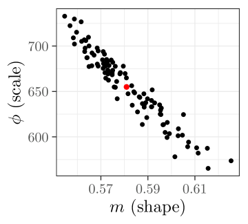
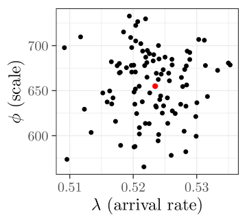
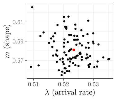
Refer to caption — (a) Shape versus scale

The parameter estimates are shown in Figure 1. The estimated parameters of the ${\mathbb{P}}_{k}$ models, $k=1,\ldots,100$ , are in black, while the estimated parameters of ${\mathbb{P}}_{C}$ are in red. We observe a negative relationship between shape and scale, and no discernible relationship between the arrival rate and the shape and scale parameters. The estimated parameters for the counterparty’s (full) model are arrival rate $\lambda_{C}=0.52$ , shape $m_{C}=0.58$ , and scale $\phi_{C}=654.98$ . 2.1 and 2.2 hold for the parameter estimates for the models ${\mathbb{P}}_{k}$ , $k=1,\ldots,100$ and ${\mathbb{P}}_{C}$ .

Using these estimated models, we implement the optimal risk sharing strategy. We simulate the jump process $\int_{0}^{t}\!\int_{{\mathds{R}}_{+}}\!\!\ln\left((1+\eta)\frac{v_{C}(\xi)}{v_{k}(\xi)}\right)N(d\xi,ds)$ , and then compute the values of $Z^{*}_{k}$ , $k=1,\ldots,100,C$ , and $X^{*}$ using Proposition 3.3. We simulate 10,000 paths of the processes from $t=0$ to $t=T=5$ . We assume that the counterparty’s safety loading is $\eta=0.12$ , the insurer’s income is $c=5{,}550$ , the weights are all equal at $\pi_{k}=1/100$ for $k=1,\ldots,100$ , $\pi_{C}=0$ , and the initial value of $X$ is $x=5{,}000$ . Setting $\pi_{C}=0$ means that the insurer does not use the counterparty’s model.

Figure 2 shows kernel density estimates of the distribution of the insurer’s terminal wealth $X_{T}$ under four scenarios.

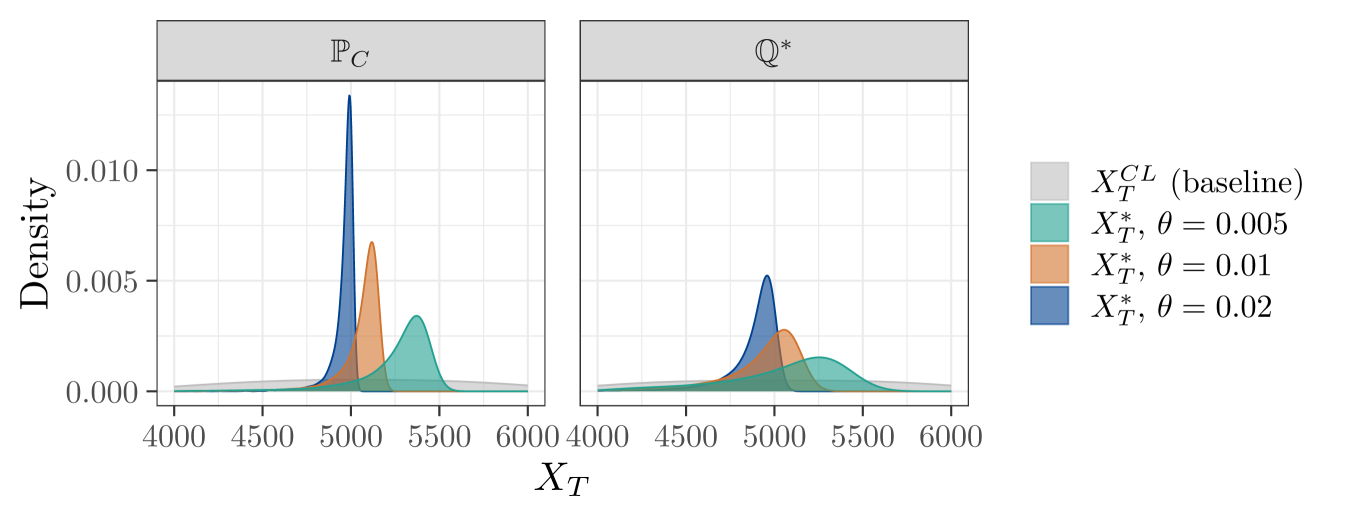
First, if the insurer does not engage in risk sharing (grey), their losses follow a Cramér-Lundberg process, $X^{CL}_{t}$ . The variance of the terminal wealth $X^{CL}_{T}$ is high, resulting in the density curve appearing nearly flat. The other three scenarios show the distribution of the terminal wealth under the optimal strategy, $X_{T}^{*}$ , for different values of the model penalization parameter $\theta$ : $\theta=0.005$ (turquoise), $\theta=0.01$ (orange), and $\theta=0.02$ (dark blue). As $\theta$ increases, the insurer’s optimal strategy puts more emphasis on variance reduction: the variance gets smaller under both ${\mathbb{P}}_{C}$ and ${\mathbb{Q}}^{*}$ , while the mean decreases under ${\mathbb{P}}_{C}$ . Estimated values of the mean and variance are given in Table 1, which shows the effect of $\theta$ on the variance and mean. For example, if $\theta=0.005$ , the variance of $X_{T}^{*}$ under ${\mathbb{P}}_{C}$ is about 89 thousand, a substantial reduction from the variance of $X^{CL}_{T}$ under ${\mathbb{P}}_{C}$ , which is about 25.8 million. This comes at a cost of a reduction in the mean under ${\mathbb{P}}_{C}$ , which falls from 7,853 to 5,239.

	${\mathbb{P}}_{C}$		${\mathbb{Q}}^{*}$
	mean	variance	mean	variance
no risk sharing	7,853	25,780,268	4,865	28,873,900
$\theta=0.005$	5,239	88,659	4,865	842,115
$\theta=0.01$	5,052	22,165	4,865	210,529
$\theta=0.02$	4,959	5,541	4,865	52,632

Table 1: The mean and variance of

X_{T}

for different values of

\theta

under

{\mathbb{P}}_{C}

and

{\mathbb{Q}}^{*}

. The mean of

X_{T}

and the variance of

X_{T}

with no risk sharing are computed exactly, while the remaining variances are estimated numerically using 10,000 simulations. The other parameters are

\eta=0.12

c=5{,}550

\pi_{k}=1/100

for

k=1,\ldots,100

\pi_{C}=0

x=5{,}000

, and

T=5

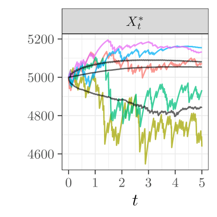
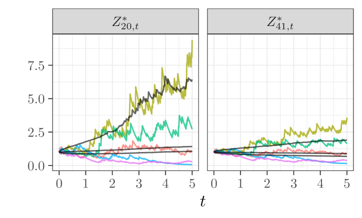
We next illustrate the behaviour of $X^{*}$ and selected $Z_{k}^{*}$ over time. Figure 3 shows five selected paths of $X^{*}$ and of two $Z^{*}$ variables under ${\mathbb{P}}_{C}$ , as well as the mean (middle black line), the mean plus standard deviation of the paths above the mean (upper black line), and the mean minus standard deviation of the paths below the mean (lower black line). We recall that the $Z^{*}$ processes are the process versions of the Radon-Nikodym derivatives between each reference model ${\mathbb{P}}_{k}$ and the optimal model ${\mathbb{Q}}^{*}$ . The selected $Z^{*}$ variables correspond to model 20 (parameters $\lambda_{20}=0.51$ , $m_{20}=0.56$ , $\phi_{20}=697.68$ ) and model 41 (parameters $\lambda_{41}=0.54$ , $m_{41}=0.57$ , $\phi_{41}=678.55$ ). We observe that when shape and scale parameters are closer to those of ${\mathbb{Q}}^{*}$ ( $m_{C}=0.5809$ , $\phi_{C}=654.98$ ), the paths of the corresponding $Z^{*}$ process are closer to 1, meaning these models are not distorted as much. The negative linear relationship between $X^{*}$ and the $Z^{*}$ s is also apparent, with the lower paths (yellow and green) of $X^{*}_{t}$ being the upper paths on $Z^{*}_{20,t}$ and $Z^{*}_{41,t}$ , and the upper paths (purple and blue) of $X^{*}_{t}$ being the lower paths on $Z^{*}_{20,t}$ and $Z^{*}_{41,t}$ .

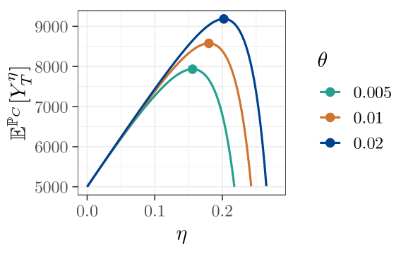
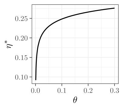
Finally, we consider the counterparty’s problem, as discussed in Section 5. Using the full 101 estimated models and the same parameters with $y=5{,}000$ and $T=5$ , we compute (24) numerically. Figure 4a shows the counterparty’s expected wealth under their probability measure ${\mathbb{P}}_{C}$ as a function of the safety loading $\eta$ for three values of $\theta$ : $\theta=0.02$ (dark blue), $\theta=0.01$ (orange), and $\theta=0.005$ (turquoise). The optimal safety loading, $\eta^{*}$ , is found numerically and denoted by a dot. We see that in these cases ${\mathbb{E}}^{{\mathbb{P}}_{C}}[Y_{T}^{\eta}]$ is concave in $\eta$ , and therefore $\eta^{*}$ is uniquely identified. Figure 4b plots the optimal safety loading $\eta^{*}$ , found numerically, as a function of $\theta$ . We see that the optimal safety loading is increasing as the model penalization parameter, $\theta$ , increases. As we have observed that increasing the model penalization parameter reduces the variance of the insurer’s terminal wealth, the interpretation is that as the insurer demands less variance of their terminal wealth, the counterparty charges a higher premium.

7 Conclusion

We study a novel risk sharing problem where an agent wishes to maximize their expected wealth under ambiguity subject to a chi-squared model ambiguity penalization. The general problem allows for the inclusion of multiple reference models, which could be used in various model uncertainty applications, such as risk scenarios linked to climate change or other extreme risks. This criterion generalizes the monotone mean-variance preferences of [19, 20], and includes it as a special case.

We solve this problem and find explicit solutions for the insurer’s optimal risk sharing strategy, optimal decision measure, and optimal wealth process. We show that the optimal wealth process $X^{*}$ depends linearly on the auxiliary processes $Z^{*}_{k}$ , $k\in{\mathcal{I}}$ , which are the process versions of the Radon-Nikodym derivatives from each reference measure ${\mathbb{P}}_{k}$ to the optimal measure ${\mathbb{Q}}^{*}$ . Using this relationship, we determine the mean and variance of $X^{*}$ under ${\mathbb{Q}}^{*}$ , and find that the model penalization parameter $\theta$ penalizes the variance of the insurer’s optimal wealth process. Furthermore, we show that the optimal decision measure, ${\mathbb{Q}}^{*}$ , depends on the model used by the counterparty and the counterparty’s premium, while the optimal risk sharing strategy depends on the model penalization parameter $\theta$ , the counterparty’s premium, and the auxiliary processes $Z^{*}_{k}$ , $k\in{\mathcal{I}}$ .

There are multiple avenues for future work stemming from this problem. First, this criterion could be applied to other contexts by changing the wealth process of the agent. Our focus here has been on model uncertainty applied to a jump process, corresponding to different scenarios for losses. The work could be expanded to consider Lévy-Itô processes more generally, though then one would have to consider ambiguity about joint models for both the diffusive and jump terms. It could also be extended to consider the minimally distorted stochastic process according to the chi-squared divergence given moment constraints, such as is done in [14] with the Kullback-Leibler divergence. Future works could also consist of using different divergences, other than Kullback-Leibler and chi-squared, to penalize model ambiguity, and determine how the divergence affects the insurer’s optimal strategy. Furthermore, while we explored the counterparty’s perspective in Section 5, this work could be further extended to a Stackelberg game framework as in [5], where both agent’s perspectives are fully considered.

Acknowledgements

EK is supported by an NSERC Canada Graduate Scholarship-Doctoral. SJ and SP would like to acknowledge support from the Natural Sciences and Engineering Research Council of Canada (grants RGPIN-2018-05705 and RGPIN-2024-04317, and DGECR-2020-00333, RGPIN-2020-04289). SP also acknowledges support from the Canadian Statistical Sciences Institute (CANSSI).

References

[1] Tomas Björk, Mariana Khapko and Agatha Murgoci “Time-Inconsistent Control Theory with Finance Applications”, Springer Finance Springer Cham, 2021 DOI: 10.1007/978-3-030-81843-2
[2] Jose Blanchet and Karthyek Murthy “Quantifying Distributional Model Risk via Optimal Transport” In Mathematics of Operations Research 44.2, 2019, pp. 565–600 DOI: 10.1287/moor.2018.0936
[3] Jose Blanchet, Henry Lam, Qihe Tang and Zhongyi Yuan “Robust Actuarial Risk Analysis” In North American Actuarial Journal 23.1 Routledge, 2019, pp. 33–63 DOI: 10.1080/10920277.2018.1504686
[4] Ben Bolker and R Development Core Team “bbmle: Tools for General Maximum Likelihood Estimation” R package version 1.0.25.1, 2023 URL: https://CRAN.R-project.org/package=bbmle
[5] Lv Chen and Yang Shen “On a new paradigm of optimal reinsurance: a stochastic Stackelberg differential game between an insurer and a reinsurer” In ASTIN Bulletin 48.2 Cambridge University Press, 2018, pp. 905–960 DOI: 10.1017/asb.2018.3
[6] Lv Chen, David Landriault, Bin Li and Danping Li “Optimal dynamic risk sharing under the time-consistent mean-variance criterion” In Mathematical Finance 31.2, 2021, pp. 649–682 DOI: https://doi.org/10.1111/mafi.12299
[7] R.. Corless et al. “On the Lambert $W$ function” In Advances in Computational Mathematics 5.1, 1996, pp. 329–359 DOI: 10.1007/BF02124750
[8] Jinye Du and Moris S. Strub “Optimal strategies and values for monotone and classical mean-variance preferences coincide when asset prices are continuous” In Operations Research Letters 57, 2024, pp. 107204 DOI: 10.1016/j.orl.2024.107204
[9] Alison L Gibbs and Francis Edward Su “On choosing and bounding probability metrics” In International statistical review 70.3 Wiley Online Library, 2002, pp. 419–435 DOI: 10.1111/j.1751-5823.2002.tb00178.x
[10] Lars Peter Hansen and Thomas J. Sargent “Robustness” Princeton University Press, 2008
[11] Ying Hu, Xiaomin Shi and Zuo Quan Xu “Constrained Monotone Mean-Variance Problem with Random Coefficients” In SIAM Journal on Financial Mathematics 14.3, 2023, pp. 838–854 DOI: 10.1137/22M154418X
[12] Sebastian Jaimungal and Silvana M. Pesenti “Kullback-Leibler Barycentre of Stochastic Processes”, 2024 DOI: 10.48550/arXiv.2407.04860
[13] Emma Kroell, Sebastian Jaimungal and Silvana M. Pesenti “Optimal robust reinsurance with multiple insurers” In Scandinavian Actuarial Journal 0.0 Taylor & Francis, 2024, pp. 1–31 DOI: 10.1080/03461238.2024.2431539
[14] Emma Kroell, Silvana M. Pesenti and Sebastian Jaimungal “Stressing dynamic loss models” In Insurance: Mathematics and Economics 114, 2024, pp. 56–78 DOI: 10.1016/j.insmatheco.2023.11.002
[15] Bohan Li and Junyi Guo “Optimal reinsurance and investment strategies for an insurer under monotone mean-variance criterion” In RAIRO-Operations Research 55.4 EDP Sciences, 2021, pp. 2469–2489 DOI: 10.1051/ro/2021114
[16] Bohan Li, Junyi Guo and Xiaoqing Liang “Optimal Monotone Mean-Variance Problem in a Catastrophe Insurance Model” In Methodology and Computing in Applied Probability 27.1, 2025, pp. 7 DOI: 10.1007/s11009-024-10134-6
[17] Bohan Li, Junyi Guo and Linlin Tian “Optimal investment and reinsurance policies for the Cramér–Lundberg risk model under monotone mean-variance preference” In International Journal of Control 97.6 Taylor & Francis, 2024, pp. 1296–1310 DOI: 10.1080/00207179.2023.2204384
[18] Yuchen Li, Zongxia Liang and Shunzhi Pang “Comparison Between Mean-Variance and Monotone Mean-Variance Preferences Under Jump Diffusion and Stochastic Factor Model” In Mathematics of Operations Research 0.0, 2024, pp. null DOI: 10.1287/moor.2022.0331
[19] Fabio Maccheroni, Massimo Marinacci and Aldo Rustichini “Ambiguity Aversion, Robustness, and the Variational Representation of Preferences” In Econometrica 74.6 [Wiley, Econometric Society], 2006, pp. 1447–1498 URL: http://www.jstor.org/stable/4123081
[20] Fabio Maccheroni, Massimo Marinacci, Aldo Rustichini and Marco Taboga “Portfolio Selection with Monotone Mean-Variance Preferences” In Mathematical Finance 19.3, 2009, pp. 487–521 DOI: 10.1111/j.1467-9965.2009.00376.x
[21] Pascal J. Maenhout “Robust Portfolio Rules and Asset Pricing” In The Review of Financial Studies 17.4, 2004, pp. 951–983 DOI: 10.1093/rfs/hhh003
[22] Sure Mataramvura and Bernt Øksendal “Risk minimizing portfolios and HJBI equations for stochastic differential games” In Stochastics: An International Journal of Probability and Stochastic Processes 80.4 Taylor & Francis, 2008, pp. 317–337 DOI: 10.1080/17442500701655408
[23] Georg Pflug and David Wozabal “Ambiguity in portfolio selection” In Quantitative Finance 7.4 Routledge, 2007, pp. 435–442 DOI: 10.1080/14697680701455410
[24] Philip E. Protter “Stochastic Integration and Differential Equations”, Stochastic Modelling and Applied Probability Springer Berlin, Heidelberg, 2005 DOI: 10.1007/978-3-662-10061-5
[25] Jorge Segura-Gisbert, Josep Lledó and Jose M. Pavı́a “Dataset of an actual motor vehicle insurance portfolio” In European Actuarial Journal, 2024 DOI: 10.1007/s13385-024-00398-0
[26] Jorge Segura-Gisbert, Josep Lledó and Jose M. Pavı́a “Dataset of an actual motor vehicle insurance portfolio.” Mendeley Data, V2, 2024 DOI: 10.17632/5cxyb5fp4f.2
[27] Yang Shen and Bin Zou “Short Communication: Cone-Constrained Monotone Mean-Variance Portfolio Selection under Diffusion Models” In SIAM Journal on Financial Mathematics 13.4, 2022, pp. SC99–SC112 DOI: 10.1137/22M1487527
[28] Xiaomin Shi and Zuo Quan Xu “Constrained monotone mean–variance investment-reinsurance under the Cramér–Lundberg model with random coefficients” In Systems & Control Letters 188, 2024, pp. 105796 DOI: 10.1016/j.sysconle.2024.105796
[29] Moris S. Strub and Duan Li “A note on monotone mean–variance preferences for continuous processes” In Operations Research Letters 48.4, 2020, pp. 397–400 DOI: 10.1016/j.orl.2020.05.003
[30] Jakub Trybuła and Dariusz Zawisza “Continuous-Time Portfolio Choice Under Monotone Mean-Variance Preferences—Stochastic Factor Case” In Mathematics of Operations Research 44.3, 2019, pp. 966–987 DOI: 10.1287/moor.2018.0952
[31] Yu Yuan, Zhibin Liang and Xia Han “Robust reinsurance contract with asymmetric information in a stochastic Stackelberg differential game” In Scandinavian Actuarial Journal 2022.4 Taylor Francis, 2022, pp. 328–355 DOI: 10.1080/03461238.2021.1971756
[32] Yan Zeng, Danping Li and Ailing Gu “Robust equilibrium reinsurance-investment strategy for a mean–variance insurer in a model with jumps” In Insurance: Mathematics and Economics 66, 2016, pp. 138–152 DOI: 10.1016/j.insmatheco.2015.10.012

	$\displaystyle f(t,X^{}_{t},\boldsymbol{Z}^{}_{t})=$	$\displaystyle\,f(0,X^{}_{0},\boldsymbol{Z}^{}_{0})+\int_{0}^{t}\frac{\partial f}{\partial s}(s,X^{}_{s^{-}},\boldsymbol{Z}^{}_{s^{-}})\,ds$
		$\displaystyle+\int_{0}^{t}\frac{\partial f}{\partial x}(s,X^{}_{s^{-}},\boldsymbol{Z}^{}_{s^{-}})dX^{}_{s}+\sum_{k\in{\mathcal{I}}}\int_{0}^{t}\frac{\partial f}{\partial z_{k}}(s,X^{}_{s^{-}},\boldsymbol{Z}^{}_{s^{-}})dZ^{}_{k,s}$
		$\displaystyle+\int_{0}^{t}\!\!\int_{{\mathds{R}}_{+}}\!\!\!\Big{\{}f\left(s,X^{}_{s^{-}}+\Delta X^{}_{s},\boldsymbol{Z}^{}_{s^{-}}+\Delta\boldsymbol{Z}^{}_{s}\right)-f(s,X^{}_{s^{-}},\boldsymbol{Z}^{}_{s^{-}})$
		$\displaystyle\qquad\qquad\quad-\frac{\partial f}{\partial x}(s,X^{}_{s^{-}},\boldsymbol{Z}^{}_{s^{-}})\Delta X^{}_{s}-\sum_{k\in{\mathcal{I}}}\frac{\partial f}{\partial z_{k}}(s,X^{}_{s^{-}},\boldsymbol{Z}^{}_{s^{-}})\Delta Z^{}_{k,s}\Big{\}}N(d\xi,ds)\,,$

	$\displaystyle{\mathbb{E}}^{{\mathbb{Q}}_{\beta}}_{t,x,\boldsymbol{z}}\left[\sup_{s\in[t,T]}\left\|J(s,X^{\alpha}_{s},Z^{\beta}_{s})\right\|\right]$
	$\displaystyle={\mathbb{E}}^{{\mathbb{Q}}_{\beta}}_{t,x,\boldsymbol{z}}\left[\sup_{s\in[t,T]}\left\|X_{s}^{\alpha}+\sum_{k\in{\mathcal{I}}}\frac{\pi_{k}}{2\theta}\,\ell_{k}(T-s)\,Z_{k,s}^{\beta}-\frac{1}{2\theta}-\left[(1+\eta)\int_{{\mathds{R}}_{+}}\!\!\xi\,\nu_{C}(d\xi)-c\right](T-s)\right\|\right]$
	$\displaystyle\leq{\mathbb{E}}^{{\mathbb{Q}}_{\beta}}_{t,x,\boldsymbol{z}}\left[\sup_{s\in[t,T]}\left\|X_{s}^{\alpha}\right\|\right]+\sum_{k\in{\mathcal{I}}}\frac{\pi_{k}}{2\theta}\,{\mathbb{E}}^{{\mathbb{Q}}_{\beta}}_{t,x,\boldsymbol{z}}\left[\sup_{s\in[t,T]}\left\|\ell_{k}(T-s)\,Z_{k,s}^{\beta}\right\|\right]$
	$\displaystyle\qquad+\frac{1}{2\theta}+\sup_{s\in[t,T]}\left(\left\|(1+\eta)\textstyle\int_{{\mathds{R}}_{+}}\!\!\xi\,\nu_{C}(d\xi)-c\right\|(T-s)\right)$
	$\displaystyle={\mathbb{E}}^{{\mathbb{Q}}_{\beta}}_{t,x,\boldsymbol{z}}\left[\sup_{s\in[t,T]}\left\|X_{s}^{\alpha}\right\|\right]+\sum_{k\in{\mathcal{I}}}\frac{\pi_{k}}{2\theta}\,\ell_{k}(T-t)\,{\mathbb{E}}^{{\mathbb{Q}}_{\beta}}_{t,x,\boldsymbol{z}}\left[\sup_{s\in[t,T]}\left\|\,Z_{k,s}^{\beta}\right\|\right]+\frac{1}{2\theta}+\left\|(1+\eta)\textstyle\int_{{\mathds{R}}_{+}}\!\!\xi\,\nu_{C}(d\xi)-c\right\|(T-t)\,.$

	$\displaystyle\hskip-10.00002pt{\mathbb{E}}^{{\mathbb{Q}}_{\beta}}_{t,x,\boldsymbol{z}}\left[\sup_{s\in[t,T]}\left\|X_{s}^{\alpha}\right\|\right]$
	$\displaystyle={\mathbb{E}}^{{\mathbb{Q}}_{\beta}}_{t,x,\boldsymbol{z}}\Bigg{[}\sup_{s\in[t,T]}\Bigg{\|}x+\int_{t}^{s}\left[c-(1+\eta)\int_{{\mathds{R}}_{+}}\!\!\!\alpha_{u}(\xi)\,\nu_{C}(d\xi)-\int_{{\mathds{R}}_{+}}\!\!\left[\xi-\alpha_{u}(\xi)\right]\nu_{C}(d\xi)\right]du$
	$\displaystyle\hskip 70.0001pt-\int_{t}^{s}\!\!\int_{{\mathds{R}}_{+}}\!\!\![\xi-\alpha_{u}(\xi)]\,\tilde{N}^{{\mathbb{P}}_{C}}(d\xi,du)\Bigg{\|}\Bigg{]}$
	$\displaystyle\leq x+c\,(T-t)+\|1+\eta\|\;{\mathbb{E}}^{{\mathbb{Q}}_{\beta}}_{t,x,\boldsymbol{z}}\left[\sup_{s\in[t,T]}\left\|\int_{t}^{s}\int_{{\mathds{R}}_{+}}\!\!\!\alpha_{u}(\xi)\,\nu_{C}(d\xi)du\right\|\right]$
	$\displaystyle\qquad+{\mathbb{E}}^{{\mathbb{Q}}_{\beta}}_{t,x,\boldsymbol{z}}\left[\sup_{s\in[t,T]}\left\|\int_{t}^{s}\!\!\int_{{\mathds{R}}_{+}}\!\!\!\left[\xi-\alpha_{u}(\xi)\right]\,\nu_{C}(d\xi)du\right\|\right]+{\mathbb{E}}^{{\mathbb{Q}}_{\beta}}_{t,x,\boldsymbol{z}}\left[\sup_{s\in[t,T]}\left\|\int_{t}^{s}\!\!\int_{{\mathds{R}}_{+}}\!\!\![\xi-\alpha_{u}(\xi)]\,\tilde{N}^{{\mathbb{P}}_{C}}(d\xi,du)\right\|\right]$
	$\displaystyle\leq x+c\,(T-t)+\|1+\eta\|\,{\mathbb{E}}^{{\mathbb{Q}}_{\beta}}_{t,x,\boldsymbol{z}}\left[\sup_{s\in[t,T]}\left(\int_{t}^{s}\!\!\int_{{\mathds{R}}_{+}}\!\!\!\left\|\alpha_{u}(\xi)\right\|\,\nu_{C}(d\xi)du\right)\right]$
	$\displaystyle\qquad+{\mathbb{E}}^{{\mathbb{Q}}_{\beta}}_{t,x,\boldsymbol{z}}\left[\sup_{s\in[t,T]}\left(\int_{t}^{s}\!\!\int_{{\mathds{R}}_{+}}\!\!\!\left\|\xi-\alpha_{u}(\xi)\right\|\,\nu_{C}(d\xi)du\right)\right]+{\mathbb{E}}^{{\mathbb{Q}}_{\beta}}_{t,x,\boldsymbol{z}}\left[\sup_{s\in[t,T]}\left\|\int_{t}^{s}\!\!\int_{{\mathds{R}}_{+}}\!\!\![\xi-\alpha_{u}(\xi)]\,\tilde{N}^{{\mathbb{P}}_{C}}(d\xi,du)\right\|\right]$
$\displaystyle\begin{split}&\leq x+c\,(T-t)+\|1+\eta\|\,{\mathbb{E}}^{{\mathbb{Q}}_{\beta}}_{t,x,\boldsymbol{z}}\left[\int_{t}^{T}\!\!\!\int_{{\mathds{R}}_{+}}\!\!\!\left\|\alpha_{u}(\xi)\right\|\,\nu_{C}(d\xi)du\right]\\ &\qquad+{\mathbb{E}}^{{\mathbb{Q}}_{\beta}}_{t,x,\boldsymbol{z}}\left[\int_{t}^{T}\!\!\!\int_{{\mathds{R}}_{+}}\!\!\!\left\|\xi-\alpha_{u}(\xi)\right\|\,\nu_{C}(d\xi)du\right]+{\mathbb{E}}^{{\mathbb{Q}}_{\beta}}_{t,x,\boldsymbol{z}}\left[\sup_{s\in[t,T]}\left\|\int_{t}^{s}\!\!\int_{{\mathds{R}}_{+}}\!\!\![\xi-\alpha_{u}(\xi)]\,\tilde{N}^{{\mathbb{P}}_{C}}(d\xi,du)\right\|\right]\,.\end{split}$		(22)

	$\displaystyle\hskip-10.00002pt{\mathbb{E}}^{{\mathbb{Q}}_{\beta}}_{t,x,\boldsymbol{z}}\left[\int_{t}^{T}\!\!\!\int_{{\mathds{R}}_{+}}\!\!\!\left\|\alpha_{u}(\xi)\right\|\,\nu_{C}(d\xi)du\right]$
	$\displaystyle={\mathbb{E}}^{{\mathbb{P}}_{C}}_{t,x,\boldsymbol{z}}\left[\frac{d{\mathbb{Q}}_{\beta}}{d{\mathbb{P}}_{C}}\int_{t}^{T}\!\!\!\int_{{\mathds{R}}_{+}}\!\!\!\left\|\alpha_{u}(\xi)\right\|\,\nu_{C}(d\xi)du\right]$
	$\displaystyle\leq\left({\mathbb{E}}^{{\mathbb{P}}_{C}}_{t,x,\boldsymbol{z}}\left[\left(\frac{d{\mathbb{Q}}_{\beta}}{d{\mathbb{P}}_{C}}\right)^{2}\right]\right)^{\frac{1}{2}}\left({\mathbb{E}}^{{\mathbb{P}}_{C}}_{t,x,\boldsymbol{z}}\left[\left(\int_{t}^{T}\!\!\!\int_{{\mathds{R}}_{+}}\!\!\!\left\|\alpha_{u}(\xi)\right\|\,\nu_{C}(d\xi)du\right)^{2}\right]\right)^{\frac{1}{2}}$
	$\displaystyle\leq\left({\mathbb{E}}^{{\mathbb{P}}_{C}}_{t,x,\boldsymbol{z}}\left[\left(\frac{d{\mathbb{Q}}_{\beta}}{d{\mathbb{P}}_{C}}\right)^{2}\right]\right)^{\frac{1}{2}}\left({\mathbb{E}}^{{\mathbb{P}}_{C}}_{t,x,\boldsymbol{z}}\left[\int_{t}^{T}\!\!\!\int_{{\mathds{R}}_{+}}\!\!\!\left\|\alpha_{u}(\xi)\right\|^{2}\,\nu_{C}(d\xi)du\right]\right)^{\frac{1}{2}}\left((T-t)\lambda_{C}\right)^{\frac{1}{2}}$
	$\displaystyle<\infty\,,$

	$\displaystyle\hskip-10.00002pt{\mathbb{E}}^{{\mathbb{Q}}_{\beta}}_{t,x,\boldsymbol{z}}\left[\sup_{s\in[t,T]}\left\|\int_{t}^{s}\!\!\int_{{\mathds{R}}_{+}}\!\!\![\xi-\alpha_{u}(\xi)]\,\tilde{N}^{{\mathbb{P}}_{C}}(d\xi,du)\right\|\right]$
	$\displaystyle\leq\left({\mathbb{E}}^{{\mathbb{P}}_{C}}\left[\left(\frac{d{\mathbb{Q}}_{\beta}}{d{\mathbb{P}}_{C}}\right)^{2}\right]\right)^{\frac{1}{2}}\left({\mathbb{E}}^{{\mathbb{P}}_{C}}_{t,x,\boldsymbol{z}}\left[\sup_{s\in[t,T]}\left\|\int_{t}^{s}\!\!\!\int_{{\mathds{R}}_{+}}\!\!\!\left[\xi-\alpha_{u}(\xi)\right]\,\tilde{N}^{{\mathbb{P}}_{C}}(d\xi,du)\right\|^{2}\right]\right)^{\frac{1}{2}}$
	$\displaystyle\leq K\left({\mathbb{E}}^{{\mathbb{P}}_{C}}\left[\left(\frac{d{\mathbb{Q}}_{\beta}}{d{\mathbb{P}}_{C}}\right)^{2}\right]\right)^{\frac{1}{2}}\left({\mathbb{E}}^{{\mathbb{P}}_{C}}_{t,x,\boldsymbol{z}}\left[\int_{t}^{T}\!\!\!\int_{{\mathds{R}}_{+}}\!\!\!\left\|\xi-\alpha_{u}(\xi)\right\|^{2}\,N(d\xi,du)\right]\right)^{\frac{1}{2}}$
	$\displaystyle\leq K\left({\mathbb{E}}^{{\mathbb{P}}_{C}}\left[\left(\frac{d{\mathbb{Q}}_{\beta}}{d{\mathbb{P}}_{C}}\right)^{2}\right]\right)^{\frac{1}{2}}\left({\mathbb{E}}^{{\mathbb{P}}_{C}}_{t,x,\boldsymbol{z}}\left[\int_{0}^{T}\!\!\!\int_{{\mathds{R}}_{+}}\!\!\!\left\|\xi-\alpha_{u}(\xi)\right\|^{2}\,\nu_{C}(d\xi)du\right]\right)^{\frac{1}{2}}$
	$\displaystyle<\infty,$