Model-Driven Deep Learning for Massive Multiuser MIMO Constant Envelope Precoding
Abstract
Constant envelope (CE) precoding design is of great interest for massive multiuser multi-input multi-output systems because it can significantly reduce hardware cost and power consumption. However, existing CE precoding algorithms are hindered by excessive computational overhead. In this letter, a novel model-driven deep learning (DL)-based network that combines DL with conjugate gradient algorithm is proposed for CE precoding. Specifically, the original iterative algorithm is unfolded and parameterized by trainable variables. With the proposed architecture, the variables can be learned efficiently from training data through unsupervised learning approach. Thus, the proposed network learns to obtain the search step size and adjust the search direction. Simulation results demonstrate the superiority of the proposed network in terms of multiuser interference suppression capability and computational overhead.
Index Terms:
Massive MIMO, constant envelope, precoding, deep learning, model-driven, unsupervised learningI Introduction
The massive multiuser multi-input multi-output (MIMO) system has attracted considerable attention because of its superiority in terms of spectral efficiency and reliability [1]. The base station (BS) utilizes numerous antennas to serve multiple user terminals (UTs) in the same time frequency resource. Linear precoders are usually used to mitigate multiuser interference (MUI) effectively [2]. However, for existing linear precoding algorithms, the actual implementation causes several problems when the number of antennas at the BS is large. A crucial challenge includes the dramatic increase in hardware cost and power consumption. Specifically, each transmit antenna needs to use an expensive linear power amplifier (PA) because the amplitude of the elements in the transmitted signal obtained by existing precoding algorithms, e.g., zero-forcing precoding, is unconstrained.
The type of transmitted signal that facilitates the use of most power-efficient/nonlinear PAs is a constant envelope (CE) signal, i.e., the amplitude of each symbol in the precoding vectors is limited to a constant, and the information is carried on the phase for transmission. Mathematically, the CE precoding design can be formulated as a nonlinear least squares (NLS) problem, which is non-convex and has multiple suboptimal solutions. In [3], Mohammed and Larsson proposed a sequential gradient descent (GD) algorithm. Unfortunately, this method is greatly affected by the initial value of the iteration algorithm and easily falls into a local minimum, which may reduce the MUI suppression ability dramatically. Reference [4] proposed a cross-entropy optimization (CEO) method to solve the NLS problem. Although CEO can mitigate MUI effectively, its computational complexity is large, thereby hindering its practical use. In [5], a Riemannian manifold optimization (RMO)-based conjugate gradient (CG) algorithm that achieves a tradeoff between MUI performance and computational complexity was developed. However, the RMO method still relies on a large number of iterations, which is still a considerable challenge for high-speed communication.
Recently, deep learning (DL) has made remarkable achievements in physical layer communications [6] and has been introduced into precoding [7, 8]. However, most existing DL-based precoders are designed in a data-driven approach, i.e., considering the precoder as a black-box network, thereby suffering excessively high training cost and computational overhead. Deep unfolding [9, 10, 11] is another DL technique, which expands the iterative algorithms and introduces some trainable parameters to improve the convergence speed, and has been applied to physical layer communications [12, 13]. In this letter, a model-driven neural network named CEPNet, which combines DL with the RMO-based CG algorithm, is proposed for the CE precoding. Compared with the RMO-based CG algorithm, the introduced trainable variables can be optimized efficiently through unsupervised learning. Thus, the MUI performance and computational cost of the proposed network have improved significantly. In addition, simulation results demonstrate that the CEPNet shows strong robustness to channel estimation error and channel model mismatch.
Notations—Throughout this letter, we use and to denote the set of real and complex numbers, respectively. The superscripts , , and represent transpose, Hermitian transpose, and conjugate transpose, respectively. denotes the Hadamard product between two matrices with identical size. returns the real part of its input argument. and represent the Euclidean norm and absolute value, respectively. Finally, for any vector and any positive integer , returns the th element in vector .
II System Model and Problem Formulation
We consider a downlink MIMO system, in which a BS with transmit antennas serves () single-antenna UTs. The collectively received signal, denoted by , is provided as follows:
| (1) |
where , , and denote the channel vector, transmitted vector, and additive white Gaussian noise, respectively. The total MUI energy can be expressed as
| (2) |
where denotes the information symbol vector.
CE precoding, which imposes a constant amplitude constraint on the transmitted signal at each transmit antenna, has been proposed, thereby enabling the utilization of low-cost and high energy efficient PAs. Mathematically, the design problem that considers CE precoding can be formulated as the constraint optimization problem:
| (3) | ||||
where denotes the total transmit power. Although no optimized method solves the non-convex problem (3), the RMO-based CG algorithm can solve the problem with a good trade-off in terms of MUI performance and complexity.
III CEPNet
III-A Algorithm Review
RMO has been proposed to solve the optimization problem (3) in [5], which transforms the constrained domain into a Riemannian manifold and solves the optimization problem directly on this specific manifold. We briefly review the RMO-based CG algorithm and recommend [14] for technical details about the RMO method.
Considering the constant amplitude constraint for each element of in problem (3) and assuming , the constraint domain of CE precoding problem can be transformed into a Riemannian manifold given by
| (4) |
Given a point of the th iteration, the tangent space at point is defined as . The search step size and direction of the th iteration are assumed as and , respectively. The point is obtained by projecting the point back to the manifold as follows:
| (5) | ||||
Next, we introduce how to determine the search direction and step size. Specifically, the CG algorithm is used to determine the search direction. The gradient direction in Euclidean space is denoted by , which should be projected onto the tangent space at point as
| (6) | ||||
Similarly, the search direction also needs to be projected onto the tangent plane at point as
| (7) |
Then, the search direction is given by
| (8) |
where is the weight calculated by Polak-Ribière formula as
| (9) |
In addition, the search step size restricted to the direction can be determined according to Armijo backtracking line search rule, that is,
| (10) |
where . A large step is usually initialized and attenuated by a factor of until (10) is satisfied. The RMO-based CE precoding method is summarized in Algorithm 1. We elaborate the RMO-based CEPNet design in the following subsection.
III-B CEPNet Design
Two primary factors can increase the computational overhead of Algorithm 1 significantly. First, the step that determines the search step size takes up almost half the time of one iteration, indicating an excessive and unbearable latency overhead when the number of iterations is large. Second, the projection and retraction operations in Algorithm 1 affect the convergence speed of the CG algorithm, thereby increasing computational complexity. Therefore, reducing the backtracking line search overhead when determining the step size as much as possible and adjusting the search direction appropriately to accelerate the convergence speed of the CG algorithm are crucial. To this end, we introduce trainable variables to the algorithm and employ DL tools.
Two improvements are applied to the CG algorithm for search step size and search direction:
-
1.
Given the th iteration, a trainable scalar is defined as the search step size of the iteration . All trainable scalars for the search step size constitute the set , where denotes the number of units that represent iterations. Each element of the set is randomly and uniformly initialized between and and trained using the stochastic GD (SGD) algorithm111The initialization interval is obtained by statistical analysis of the search step size determined by the traditional Armijo backtracking line search rule.. All trainable variables are fixed after training so that they can be used directly during testing without researching on the basis of the Arimijo backtracking line search rule.
-
2.
We focus on the weight calculated by Polak-Ribière formula in (9) to adjust the search direction of the iteration . In particular, we calculate according to (9) to obtain a reasonable initial weight value. In addition, a trainable scalar is defined and multiplied by to determine a new weight factor. All trainable scalars for adjusting the search direction constitute the set . Each element of the set is initialized to 1 and trained with SGD. Similarly, the weights are fixed after training.
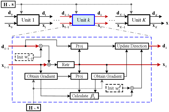
As such, we obtain a CE precoding network named CEPNet, which combines the traditional RMO-based CG algorithm with DL. The overview of the proposed DL architecture is shown in Fig. 1, in which the network inputs are and , and the output is . Each unit can be regarded as an iteration of the traditional RMO method. Each unit contains two trainable variables, and the number of total trainable variables in the proposed CEPNet is . Alternatively, each unit contains two active neural layers, and the total number of neural layers in the CEPNet shown in Fig. 1 is . On this basis, we do not recommend that the CEPNet contain too many units because excessive neural layers cause the network to be too “deep,” which may lead to tricky gradient vanishing or exploding. The proposed network is easy to train because only few trainable variables need to be optimized.
To train CEPNet, supervised learning design is inflexible and inadequate because the optimal label is unknown. Obtaining labels through existing algorithms is one approach. However, it only makes the network learn the existing algorithms. Therefore, in our design, an unsupervised learning algorithm is used to train CEPNet effectively. The set of trainable variables is denoted as . The inputs of CEPNet are and , and the transmitted vector is denoted by . To improve the robustness of the CEPNet to signal-to-noise ratio (SNR), we use MUI as the loss function directly rather than the average achievable rate or the bit-error rate (BER) that is related to the SNR. Specifically, the loss function is calculated as follows:
| (13) |
where denotes the total number of samples in the training set. and represent the information symbol and channel vectors associated with the ith symbol, respectively.
IV Experiments
IV-A Implementation Details
The CEPNet is constructed on top of the TensorFlow framework, and an NVIDIA GeForce GTX 1080 Ti GPU is used for accelerated training. The training, validation, and testing sets contain , , and samples, respectively. We perform simulation experiments with the multipath channel, and the channel vector of the th UT is determined by
| (14) |
where is the number of propagation paths of user , and denotes the complex gain of the th propagation path in the th UT’s channel, and
| (15) |
denotes the steering vector of the th user, where , , and denote the distance between two horizontally or vertically adjacent antenna elements, the carrier wavelength, and the angle of departure of the th propagation path in the th UT’s channel, respectively. The channel vector . We set . is drawn from , and is uniformly generated between and . The data sets are formed in pair. The channel vector is set as block fading, and one transmitted vector corresponds to one channel vector , where each is generated independently and each element of the transmitted vector is drawn from the 16-QAM constellation. We set for the trade-off between MUI performance and computational complexity. The set of trainable variables is updated by the ADAM optimizer [15]. The training epochs, learning rate, and batch size are set as , , and , respectively.
IV-B Performance Analysis
IV-B1 Average achievable rate
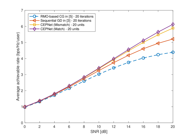
In Fig. 2, we compare the performance of the proposed CEPNet with the existing CE precoding algorithms on the average achievable rate against the SNR in a multipath channel, where the achievable rate at each UT can be calculated using [16, Eq. (43)]. The BS is equipped with transmit antennas and serves UTs. Fig. 2 indicates that the CEPNet trained with the matched multipath channel outperforms the RMO-based CG algorithm with the same number of iterations significantly, demonstrating that the proposed CEPNet can learn to reduce the total MUI through an unsupervised learning approach, i.e., the CEPNet learns to adjust the search step size and direction of each iteration appropriately through training. In addition, the CEPNet also outperforms the sequential GD algorithm with the same number of iterations at high SNRs. We infer that the CEPNet learns to deal with the channel singular issue in the multipath channel through training, while the sequential GD algorithm fails. In general, the average achievable rate performance of the CEPNet is better than the existing CE precoding algorithms in the multipath channel.
IV-B2 Bit-error rate
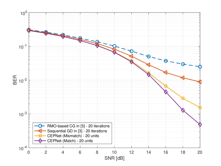
Fig. 3 compares the BER performance of the CEPNet with existing CE precoding algorithms in the multipath channel, where the BS is equipped with transmit antennas and serves UTs. In Fig. 3, the CEPNet trained with the matched channel model obtains the best BER performance among all CE precoders. Specifically, the CEPNet outperforms the RMO-based CG algorithm with the same number of iterations by approximately dB when we target SNR for . Similarly, the CEPNet outperforms the sequential GD algorithm with the same number of iterations by approximately dB when we target SNR for .
IV-B3 Computational complexity
We compare the computational overhead of the RMO-based CG algorithm, the sequential GD algorithm, and the CEPNet222We first construct the CEPNet on top of the TensorFlow framework and an NVIDIA GeForce GTX 1080 Ti GPU is used for accelerated training. Once the CEPNet converges, the parameters are stored into .csv files. The parameters of the CEPNet are obtained from the pre-stored files directly when we implement the CEPNet with MATLAB framework. with same number of iterations in Table I, where and . The aforementioned CE precoders are all implemented with MATLAB framework for fairness. Time comparison is performed on a computer with OSX 10.12, i5-6360U 2.9 GHz dual-core CPU, and 8 GB RAM.
| CE precoding algorithms | time (in seconds) |
|---|---|
| RMO-based CG – 20 iterations | 0.00079 |
| Sequential GD in [3] – 20 iterations | 0.0321 |
| Our proposed CEPNet – 20 units | 0.00036 |
The results indicate that CE precoding through the CEPNet can be executed with a lower overhead than that through the RMO-based CG algorithm because the former does not require any backtracking on the search step size. Specifically, the CEPNet with units performs approximately and times faster than the RMO-based CG algorithm with iterations and the sequential GD algorithm with iterations, respectively.
IV-C Robustness Analysis
IV-C1 Robustness to channel estimation error
In Sec. IV-B, we assume that the BS can obtain perfect channel state information (CSI) for precoding. However, considering that obtaining perfect CSI is impractical, we first investigate the robustness of the CEPNet to channel estimation error in this section. The channel estimation vector used for precoding is assumed to be given by
| (16) |
where and is drawn from . The value of measures the magnitude of the channel estimation error. The CEPNet is trained with perfect CSI. We evaluate the RMO-based CG algorithm, the sequential GD algorithm, and the CEPNet with imperfect CSI. The aforementioned CE precoding algorithms are all performed with iterations and dB.
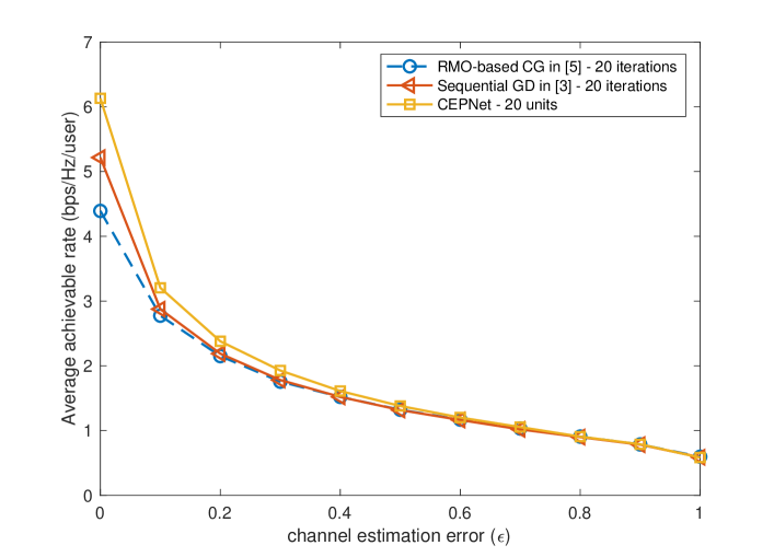
Fig. 4 illustrates the robustness of different CE precoding algorithms to the channel estimation error. The figure shows that the proposed CEPNet outperforms the RMO-based CG algorithm and the sequential GD algorithm when , which indicates that the learned variables are robust to channel estimation error. In addition, the performance of the aforementioned CE precoding algorithms is similar when because the channel estimation error is significant.
IV-C2 Robustness to channel model mismatch
We investigate the robustness of the CEPNet to channel model mismatch. Specifically, the CEPNet is trained with a Rayleigh-fading channel and deployed with a multipath channel. Each element of the Rayleigh-fading channel is drawn from . Figs. 2 and 3 indicate that the CEPNet trained with the Rayleigh-fading channel can also achieve significant gains compared with existing CE precoders in the multipath channel, which demonstrates that the learned variables are robust to channel model mismatch.
In general, the CEPNet shows strong robustness to channel estimation error and channel model mismatch. We also do not have to retrain the CEPNet if the channel variation is insignificant. However, we should retrain the CEPNet to improve performance when the channel variation amplitude is significant. Considering that the CEPNet only contains the parameter, we can retrain the CEPNet with a low overhead to adapt the changed channel.
V Conclusion
We proposed a novel model-driven DL network for multiuser MIMO CE precoding. The designed CEPNet inherited the superiority of the conventional RMO-based CG algorithm and DL technology, thereby exhibiting excellent MUI suppression capability. Simulation results demonstrated that the CEPNet could reduce the precoding overhead significantly compared with the existing CE precoding algorithms. Furthermore, the CEPNet showed strong robustness to the channel estimation error and the channel model mismatch.
References
- [1] L. Lu, G. Ye Li, A. L. Swindlehurst, A. Ashikhmin, and R. Zhang, “An overview of massive MIMO: Benefits and challenges,” IEEE J. Sel. Topics Signal Process., vol. 8, no. 5, pp. 742–758, Oct. 2014.
- [2] E. G. Larsson, F. Tufvesson, O. Edfors, and T. L. Marzetta, “Massive MIMO for next generation wireless systems,” IEEE Commun. Mag., vol. 52, no. 2, pp. 186–195, Feb. 2014.
- [3] S. K. Mohammend and E. G. Larsson, “Per-antenna constant envelope precoding for large multiuser MIMO systems,” IEEE Trans. Commun., vol. 61, no. 3, pp. 1059–1071, Mar. 2013.
- [4] J.-C. Chen, C.-K. Wen, and K.-K. Wong, “Improved constant envelope multiuser precoding for massive MIMO systems,” IEEE Commun. Lett., vol. 18, no. 8, pp. 1311–1314, Aug. 2014.
- [5] J.-C. Chen, “Low-PAPR precoding design for massive multiuser MIMO systems via Riemannian manifold optimization,” IEEE Commun. Lett., vol. 21, no. 4, pp. 945–948, Apr. 2017.
- [6] T. Wang, C.-K. Wen, H. Wang, F. Gao, T. Jiang and S. Jin, “Deep learning for wireless physical layer: Opportunities and challenges,” China Commun., vol. 14, no. 11, pp. 92–111, Nov. 2017.
- [7] A. M. Elbir and A. Papazafeiropoulos, “Hybrid precoding for multi-user millimeter wave massive MIMO systems: A deep learning approach,” IEEE Trans. Veh. Technol., vol. 69, no. 1, pp. 552–563, Jan. 2020.
- [8] W. Xia, G. Zheng, Y. Zhu, J. Zhang, J. Wang, and A. Petropulu, “A deep learning framework for optimization of MISO downlink beamforming,” IEEE Trans. Commun., vol. 68, no. 3, pp. 1866–1880, Mar. 2020.
- [9] D. Ito, S. Takabe and T. Wadayama, “Trainable ISTA for Sparse Signal Recovery,” IEEE Trans. Signal Process., vol. 67, no. 12, pp. 3113–3125, Jun. 2019.
- [10] A. Balatsoukas-Stimming and C. Studer, “Deep unfolding for communications systems: A survey and some new directions,” in Proc. IEEE SiPS, Nanjing, China, Oct. 2019, pp. 1–4.
- [11] V. Monga, Y. Li, and Y. Eldar, “Algorithm unrolling: interpretable, efficient deep learning for signal and image processing,” preprint, 2019. [Online]. Available: http://arxiv.org/abs/1912.10557.
- [12] H. He, S. Jin, C. Wen, F. Gao, G. Y. Li, and Z. Xu, “Model-driven deep learning for physical layer communications,” IEEE Wireless Commun., vol. 26, no. 5, pp. 77-83, Oct. 2019.
- [13] A. Balatsoukas-Stimming, O. Castaneda, S. Jacobsson, G. Durisi, and C. Studer, “Neural-network optimized 1-bit precoding for massive MU-MIMO,” in Proc. IEEE SPAWC, Cannes, France, Jul. 2019, pp. 1–4.
- [14] P.-A. Absil, R. Mahony, and R. Sepulchre, Optimization Algorithms on Matrix Manifolds. Princeton, NJ, USA: Princeton Univ. Press, 2009.
- [15] D. P. Kingma and J. Ba, “Adam: A method for stochastic optimization,” preprint, 2014. [Online]. Available: http://arxiv.org/abs/1412.6980.
- [16] C. Mollén, E. G. Larsson, and T. Eriksson, “Waveforms for the massive MIMO downlink: Amplifier efficiency, distortion, and performance,” IEEE Trans. Commun., vol. 64, no. 12, pp. 5050–5063, Dec. 2016.