Model for tumour growth with treatment by continuous and pulsed chemotherapy
Abstract
In this work we investigate a mathematical model describing tumour growth under a treatment by chemotherapy that incorporates time-delay related to the conversion from resting to hunting cells. We study the model using values for the parameters according to experimental results and vary some parameters relevant to the treatment of cancer. We find that our model exhibits a dynamical behaviour associated with the suppression of cancer cells, when either continuous or pulsed chemotherapy is applied according to clinical protocols, for a large range of relevant parameters. When the chemotherapy is successful, the predation coefficient of the chemotherapic agent acting on cancer cells varies with the infusion rate of chemotherapy according to an inverse relation. Finally, our model was able to reproduce the experimental results obtained by Michor and collaborators [Nature, 435, 1267 (2005)] about the exponential decline of cancer cells when patients are treated with the drug glivec.
keywords:
tumour , delay , chemotherapy1 Introduction
Cancer is the name given to a cluster of more than 100 diseases that presents a common characteristic, the disorderly growth of cells that invade tissues and organs [1, 2]. These cells may spread to other parts of the body rapidly forming tumours [3].
An important mechanism of body defence against a disease caused by a virus, bacteria or tumour is the destruction of infected cells or tumours by actived cytotoxic T-lymphocytes (CTL) cells also known as hunter lymphocytes. CTL are able to kill cells or to induce a programmed cell death (apoptosis). The biological activation process occurs efficiently when the CTL receive impulses generated by T-helper cells (). The stimuli occur through the release of cytokines. This phenomenon is not instantaneous; besides the time elapsed to convert resting T-lymphocytes in CTL, there is also a natural delay of the cytological process [4, 5]. Banerjee and Sarkar studied the dynamical behaviour of tumour and immune cells using delay differential equations [6]. They observed the existence of oscillations in tumour cells when a time delay was considered in the growth of T-cells.
A possible way to stop the growing of cancer cells is chemotherapy. That is, the treatment with a drug or combination of drugs through some protocol. There are many experimental and theoretical studies about the effects of the chemotherapy on the cells. Moreover, mathematical models have been considered to simulate the growth of cancer cells [7], as well as, tumour-immune interactions with chemotherapy [8].
In this paper we investigate a mathematical model for the growth of tumours that not only take into consideration the time delay character of the lymphocytes dynamics, but also the effect of the chemotherapy. We extend the model of Sarkar and Banerjee [6] by adding the chemotherapy, and by considering some clinically plausible protocols. Firstly, a continuous chemotherapy is analysed. Secondly, the traditional or pulsed chemotherapy protocol is analysed, in which the drug is administered periodically. According to experimental protocols, we have used both a constant amplitude [9] and an oscillatory amplitude [10] for the continuous infusion rate of chemotherapy [11].
One of our main results is to show that there are a large range of relevant parameters that lead to a successful chemotherapy. In a successful chemotherapy is that the predation coefficient of the chemotherapic agent acting on the cancer cells and the infusion rate of the chemotherapy are inversely related. For the continuous chemotherapy, we have ensured the stability of the non-cancer state (i.e., a successful chemotherapy) by calculating the Lyapunov exponents of the non-cancer solution. Finally, our model was able to reproduce the experimental results obtained by Michor and collaborators [12] about the exponential decline of cancer cells when patients are treated with the drug glivec.
2 The model
We extend a mathematical model proposed by Banerjee and Sarkar [13] including the chemotherapic agent. The model is based on the predator-prey system. The T-lymphocyte is the predator, while the tumour cell is the prey that is being attacked. The predators can be in a hunting or a resting state. The resting cells do not kill tumour cells, but they can become hunters. The activation occurs not only due to cytokines released by macrophages that absorb tumour cells, but also by direct contact between resting and tumour cells. As a result, the resting cells suffer a degradation while the hunting cells are actived. The activated cells do not return to the resting state. This way, the predator-prey model is a three dimensional deterministic system, consisting of tumour cells, hunting cells, and resting cells. We added the chemotherapic agent in the equations as a predator on both cancerous and lymphocytes cells. The time delay of about 60 days considered in our model was observed by Balduzzi and collaborators [14, 15], when they were realising experiments about lymphoblastic leukaemia. It incorporates many different phenomena in the system. It is one order of magnitude larger than the one observed in Ref. [16]. In our model, the time delay represents the total time interval for cancer cells to be identified by T-cell receptors and transfer this information to the killer cells, and the time related to the process of cytolytic information in the resting cells [16, 17]. The model is then given by
| (1) | |||||
where , and are the number of cancerous, hunting and resting cells, respectively, is the time and is the concentration of the chemotherapic agent. The cancerous and resting cells have a logistic growth. The term represents the natural death of the hunting cells. The terms and are the losses due to encounters between the cancerous and hunting cells. The term is associated with the conversion of resting to hunting state, where is the delay in the conversion. The terms with correspond to interaction of the chemotherapic agent with the cells.
Table 1 shows the parameters obtained from the literature, according to experimental evidence, and Table 2 shows the definition of some of the parameters. Table 3 presents the values that we consider in our simulations for the sake of numerical integration.
| Parameter | Definition | Value | Ref. |
|---|---|---|---|
| growth rate of malignant tumour cells | 0.18 day-1 | [18] | |
| carrying capacity of tumour cells | 5 x cells | [18] | |
| decay rate of tumour | 1.101 x | [19] | |
| cells by hunting cells | cells-1 day-1 | ||
| decay rate of hunting | 3.422 x | [19] | |
| cells by tumour cells | cells-1 day-1 | ||
| death rate of hunting cells | 0.0412 day-1 | [19] | |
| growth rate of resting cells | 0.0245 day-1 | [6] | |
| time delay in conversion from resting cells to hunting cells | 45.6 day | [6] | |
| carrying capacity of resting cells | 1 x cells | [6] | |
| conversion rate from | 6.2 x | [19] | |
| resting to hunting cells | cells-1 day-1 |
| Parameter | Definition | Ref. |
|---|---|---|
| predation coefficients of chemotherapic | [11] | |
| agent on cells (C, H, R) | ||
| determine the rate at which C, H, R, | [11] | |
| in the absence of competition and | ||
| predation, reach carrying capacities | ||
| represent the combination rates of the | [11] | |
| chemotherapic agent with the cells | ||
| represents the infusion rate | [11] | |
| of chemotherapy | ||
| washout rate of chemotherapy | [11] |
Introducing the following dimensionless variables
| (2) |
where is the total carrying capacity and is equal 1 mg . Combining (2) with (1), and relabelling the variables , , , , as t, C, H, R, Z, respectively, and the parameters , , , , , , , , , , , , , , , , , , as , , , , , , , , , , , , , , , , , , , respectively, we obtain the same equations for , and . However, the equation for presents a small alteration,
| (3) | |||||
where we consider
| (4) | |||||
| Parameter | Value | Parameter | Value |
|---|---|---|---|
| 0.18 | 1/3 | ||
| 1.6515 | 5.133 x | ||
| 0.0412 | 0.0245 | ||
| 45.6 | 2/3 | ||
| 9.3 x | 1 x | ||
| 1 x | 1 x | ||
| 1 x | 1 x | ||
| 1 x | 0.1 | ||
| 0.1 | 0.1 | ||
| 0 - | 0.2 |
3 Continuous chemotherapy
In this section we consider the continuous application of chemotherapy, without pause or interruption. That is, the value of the is constant in time.
3.1 Cancer suppression
We consider the following initial conditions: , , and . These initial conditions are in the limit cycle region of the model solution. The periodic behaviour implies that the tumor levels oscillate around a fixed point, a clinically observed behaviour known as Jeff’s phenomenon. One cancer cell in the model (1) is equal to in the dimensionless model. Our main aim is to find parameters that make the chemotherapy successfully suppress cancer, but that preserves the lymphocytes population.
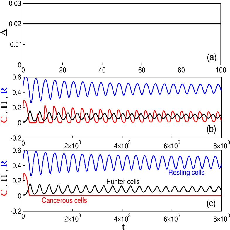
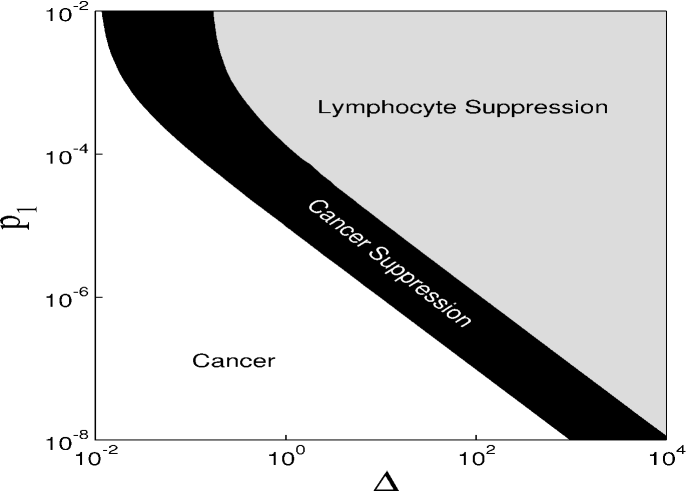
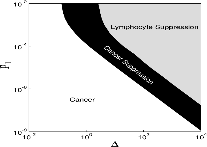
Figure 1 displays the time evolution of the dimensionless quantities and variables. Figure 1(a) shows the behaviour of the infusion rate of chemotherapy. For [Fig. 1(b)] there is no cancerous suppression and the system presents stable oscillatory behaviour. If we increase the value of to 0.025 [Fig. 1(c)], the system may present cancerous suppression without the disappearance of lymphocytes. However, for larger , not only the cancer cells, but also lymphocytes disappear. To obtain a global picture of the parameters leading to different behaviour of our model, we construct the parameter space shown in Figure 2, for the parameters and the predation coefficient of chemotherapy, . For the rate of cancer cells proliferation is unaffected by the chemotherapic agent. This case may be interpreted as the use of inappropriated drugs or mechanisms related to drug resistance. When is not null, there is drug-induced killing of cancer cells. These parameters are important due to the fact that they are directly related to the chemotherapy used in the treatment of cancer. We can identify three behaviours in this parameter space. In the white region there are cancer cells. The suppression of cancer occurs for the parameters in the black region. The grey region presents an undesired situation, the suppression of lymphocytes. Therefore, we observe that it is possible to achieve cancerous suppression by increasing infusion rate of the chemotherapy to a high enough value, but the threshold depends on the value of . For the parameters and in the black region the number of malignant tumour cells goes to zero preserving the immune cells. When the number of cancer cells is zero, the treatment can stop and the tumour will not return.
3.2 Lyapunov exponents
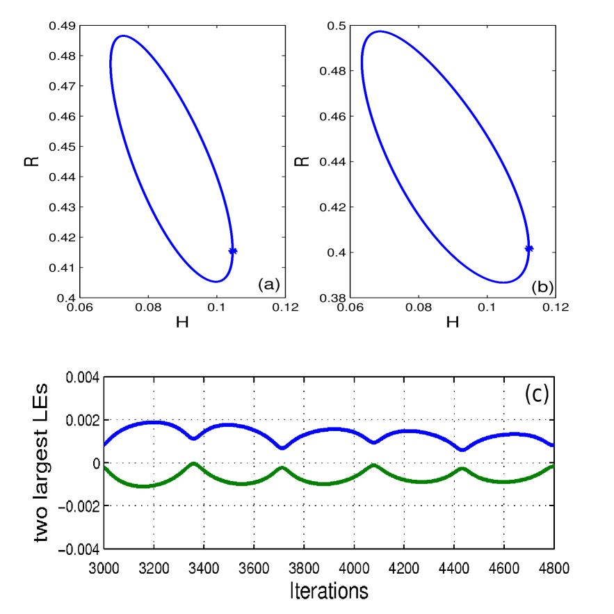
To verify whether the suppression of cancer () is stable, that is, the cancer will not return after its elimination, we calculate the spectra of Lyapunov exponents of our model with time delay. We present only the values of the two largest Lyapunov exponents () at time . We are interested in the maximal value of . Firstly, we use a value of , in that the therapy does not eliminate the cancer. In this case, the system oscillates in a stable limit cycle (Fig. 3a). The largest Lyapunov exponent is about and the second largest negative. To determine that no cancer is an unstable solution of the model, we calculate the conditional Lyapunov exponents of the whole system but requiring the trajectory to lie in the subspace . We obtain one positive Lyapunov exponent [20], which must be associated with the stability in this subspace since the Lyapunov exponents of the 3D reduced version of our model in (3), without the variable for , are all negative. In other words, if , cancer will certainly not be eliminated.
For , not only the cancer can be eliminated, but also the dynamics in the subspace is stable. Figure 3(b) shows that the behaviour of the system is a limit cycle. The result of the two largest Lyapunov exponents for the case is given in Figure 3(c). The maximum values and , for , are 0.0015 and -0.0001. Notice that this is only an upper bound for the real value and it indicates that the real value, whatever it is, needs necessarily to be smaller than 0.0015, a small number that we interpret as being 0, as required for a limit cycle.
4 Pulsed chemotherapy
Often chemotherapy treatments are carried out in cycles. The repeated application of drugs for a short time is a typical protocol for chemotherapy, called pulsed chemotherapy [21]. For example, in this protocol, one may use the drug doxorubicin combined with other drugs to treat some types of cancer. The chemotherapy with these drugs is given through cycles of treatment according to the type of cancer [22].
In the following, we will consider two clinical protocols for the chemotherapy with respect to their dependence on the rate . One protocol is to administer the drug at a constant and the other for two values of this rate ( and ), both of which have been applied with a determined period between two chemotherapic sessions. Our aim is to obtain the cancer suppression, while preserving the lymphocytes.
4.1 First protocol
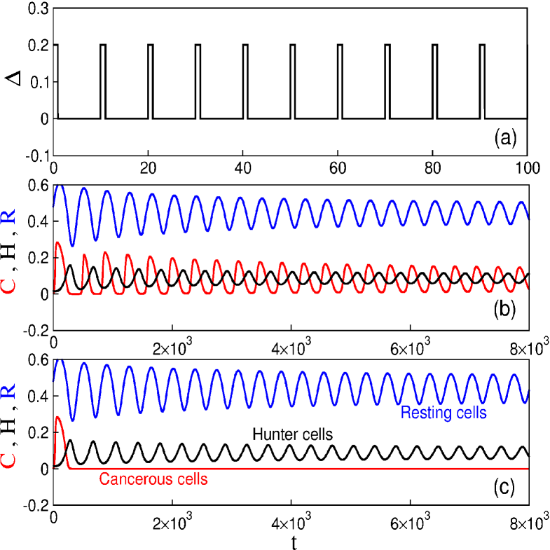
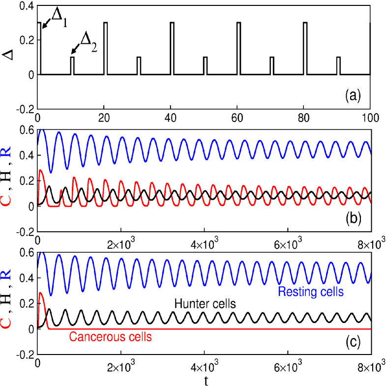
Figure 4(a) exhibits the drug injection pattern for the first protocol. When , , and parameters in Table 3, the tumour cell population does not vanish, as depicted in Figure 4(b). However, considering the same period , it is possible to obtain cancer suppression for (Fig. 4c).
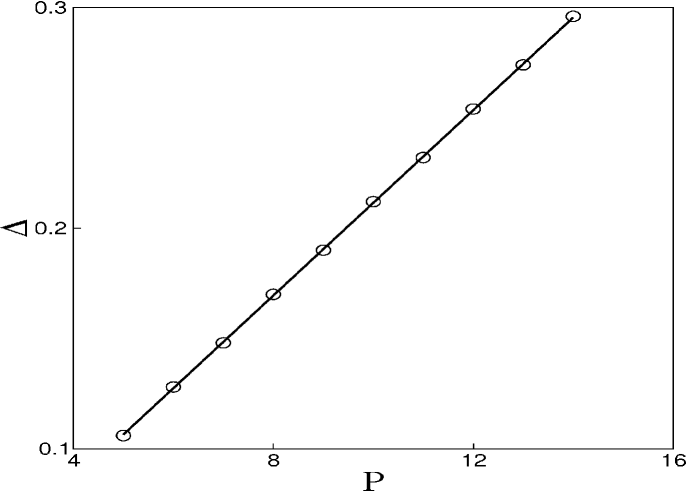
The drugs have specific protocols of application according to the type of tumour. For this reason we study the period of the drug injection. Figure 5 exhibits the time interval of the pulsed chemotherapy, where the points are used to denote the minimum value of the rate in which the cancer suppression occurs. When increases, it is necessary to increase the intensity of the chemotherapy to obtain cancer suppression. As a matter of fact, the infusion rate versus the period shows a linear increase with the critical value of as grows, .
To verify the effect of the period on the behaviour of our model, we show the parameter space in Fig. 6, similar to the one shown in Figure 2, but considering pulsed chemotherapy with a period equal to 10. We also see the three behaviours: white regions represent parameters that lead to cancer, black regions represent parameters that lead to the suppression of cancer, and the grey region represent parameters that lead to the suppression of lymphocytes. Therefore, it is still possible to obtain a successful chemotherapy. However, the threshold of values of and leading to a successful chemotherapy are larger in the pulsed chemotherapy with , then these threshold values for a continuous chemotherapy. This is a realistic behaviour observed in treatments that prescribe chemotherapic drugs in a continuous or pulsed way.
4.2 Second protocol
Another case for the pulsed chemotherapy consists in infusions of drugs with different concentrations and periods. There is recent research about the successful rate of each type of pulsed chemotherapy [10]. For instance, the treatment for colon cancer adding oxaliplatin to bolus, fluorouracil mixed with leucovorin has been used with different infusion rates [10]. Due to clinical treatment described in the literature, we consider to oscillate between two values.
Figure 7(a) shows the drug injection pattern with , , and . For these values of the cancer cells do not disappear but they oscillate at regular intervals (Fig. 7b). On the other hand, fixing and increasing the cancer is suppressed, as can be observed in Figure 7(c).
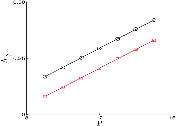
When the infusion rate is constant and chemotherapy sessions are periodically repeated, the cancer suppression depends on the time interval . For this reason we fix and vary and that results in the successful treatment of cancer. As a result, we see in Figure 8, the lines represent the minimal values of for a given that lead to cancer suppression. The circles are for and the squares are for . Fixing and varying , we obtain the same result.
Through the Figure 5 and Figure 8, we can see a linear relation between and . Defining the frequency as , the infusion rate versus the frequency will show a linear decreases with the critical value of as decreases, . This way, when tuning the frequency, the value of the rate in that the cancer suppression occurs is altered.
The drug Diethylstilbestrol to prostate cancer can be used in treatment by continuous or pulsed chemotherapy. In a continuous treatment may be administered 50 mg (oral) per day, every day, while in a pulsed treatment this drug may be administered 500 mg (infusion) once per week, many weeks. Comparing, we can see that the value of the pulsed is ten times the value of the continuous. Then, the values that we used are in accordance with realistic values.
4.3 Exponential decline of cancer cells
Michor and collaborators [12] analysed 169 chronic myeloid leukaemia patients, a cancer of the white blood cell, or leukocytes. They studied the dynamics of different treatment responses to tyrosine kinase inhibitor imatinib, which is also known as glivec. The imatinib is used to treat some types of leukaemia and soft tissue sarcoma. The treatment with this drug causes the death of cancer cells by inhibiting the signals exchanged by the cancer cells responsible to produce the growth and the division of the cancer cells.
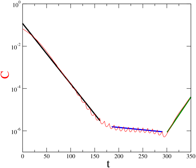
In Ref. [12] was showed that a successful therapy using imatinib leads to a biphasis exponential decline of leukaemic cells in time. The value of the first slope (quantifying the exponential time decay rate of cancer cells) is approximately , and represents the death of leukaemic differentiated cells. The second slope is around , and is due to the death of leukaemic progenitors. If the imatinib therapy is interruped the slope is approximately . Without imatinib the differentiated leukaemic cells arise from leukaemic stem cells. Figure 9 shows the slopes obtained through the model (2). We consider , , and two values for . We use for the time interval that produces the first slope (black line) , and for the time interval that produces the second slope (blue line) . For , time interval that produces the third slope (green line) there is not chemotherapy. As a result, we obtain the slopes , , and , which are remarkably similar with the slopes obtained in Ref. [12].
In our model, the case without therapy can be simulated by setting the parameter equal to zero. This parameter can be also used to simulate a case where the cancer cells become resistante to the drug. The leukaemic cells may present resistance to imatinib therapy. Resistance can be modelled decreasing the effect of chemotherapy to cancer cells (i.e., decreasing ), while leaving the effect on immune cells constant (maintaining and ).
5 Conclusions
We propose a delay differential equations model for the evolution of cancer under the attack of both the immune system and chemotherapy. The novelty in this model is the introduction of the chemotherapy and the adjustment of parameters according to recent experimental evidence. We considered some types of protocols aiming at the cancer suppression.
We studied a continuous administration of drugs. The solutions of the system are stable, presenting a limit cycle behaviour. We identified domains of cancer suppression for a wide parameter range of the predation coefficient of the chemotherapic agent and of the continuous infusion rate of chemotherapy, . Our main results in this session was to show that (i) and that lead to a successful cancer treatment (elimination of cancer cells) are inversely related; (ii) too large values of and eliminate cancer but also eliminate the lymphocytes.
The success of the chemotherapic treatment is highly dependent on the values of the parameters and , responsible for the interactions between the tumour and the drug. By varying we were able to obtain the biphasic exponential decline observed in chronic myeloid leukaemia [12]. Moreover, the variation of permits to simulate cases in which the tumour develops drug resistance.
We examined the behaviour of the cancer cells with pulsed chemotherapy and its dependence on the chemotherapic dosing regime. We verified the possibility of cancer suppression through two clinical protocols. In fact, we investigated infusions of drugs with equal and different concentrations. The protocol with different concentrations is more used in the case of drug combination. Our results enabled us to predict the values of the relevant parameters for cancer suppression through protocols related to the treatment of ill people.
Acknowledgements
This study was partially supported by the following Brazilian Government Agencies: CNPq, CAPES, FAPESP and Fundação Araucária. HPR, MSB, CG acknowledge the RSE-NSFC (443570/NNS/INT-61111130122). K. C. Iarosz acknowledges CAPES Foundation, Ministry of Education of Brazil, Brasília - Processo n. 1965/12-3.
References
- [1] Anderson, G.R., Stoler, D.L., Brenner, B.M., 2001. Cancer: the evolved consequence of a destabilized genome. Bioessays 23 (11), 1037-1046.
- [2] Brú, A., Albertos, S., Subiza, J.L, García-Asenjo, J. L., Brú, I., 2003. The universal dynamics of tumor growth. Biophysical Journal 85 (5), 2948-2961.
- [3] Baserga, R., 1965. The relationship of the cell cycle to tumor growth and control of cell division: A review. Cancer Research 25 (5), 581-593.
- [4] Wodarz, D., Klenerman, P., Nowak, M., 1998. Dynamics of cytotox T-lymphocyte exhaustion. Proceedings of the Royal Society B: Biological Sciences 265, 191-203.
- [5] Iarosz, K.C., Martins, C.C., Batista, A.M., Viana, R.L., Lopes, S.R., Caldas, I.L., Penna, T.J.P., 2011. On a cellular automaton with time delay for modelling cancer tumors. Journal of Physics: Conference Series 285, 012015.
- [6] Banerjee, S., Sarkar, R.R., 2008. Delay-induced model for tumor-immune interaction and control of malignant tumor growth. BioSystems 91, 268-288.
- [7] Liu, D., Ruan, S., Zhu, D., 2012. Stable periodic oscillations in a two-stage cancer model of tumor and immune system interactions. Mathematical Biosciences and Engineering 9 (2), 347-368.
- [8] De Pillis, L.G., Gu, W., Fister, K.R., Head, T., Maples, K., Murungan, A., Neal, T., Yoshida, K., 2007. Chemotherapy for tumors: an analysis of the dynamics and a study of quadratic and linear optimal controls. Mathematical Biosciences 209 (1), 292-315.
- [9] Ahn, I., Park, J., 2011. Drug scheduling of cancer chemotherapy based on natural actor-critic approach. BioSystems 106, 121-129.
- [10] Kuebler, J.P., Wieand, H.S., O’Connell, M.J., Smith, R.E., Colangelo, L.H., Yothers, G., Petrelli, N.J., Findlay, M.P., Seay, T.E., Atkins, J.N., Zapas, J. L., Goodwin, J.W., Fehrenbacher, L., Ramanathan, R.K., Conley, B.A., Flynn, P.J., Soori, G., Colman, L.K., Levine, E.A., Lanier, K.S., Wolmark, N., 2007. Oxaliplatin combined with weekly bolus fluorouracil and leucovorin as surgical adjuvant chemotherapy for stage II and III colon cancer: Results from NSABP C-07. Journal of Clinical Oncology 25 (16), 2198-2204.
- [11] Pinho, S.T.R., Freedman, H.I., Nani, F., 2002. A chemotherapy model for the treatment of cancer with metastasis. Mathematical and Computer Modelling, 36, 773-803.
- [12] Michor, F., Hughes, T.P., Iwasa, Y., Brandford, S., Shah, N.P., Swayers, C.L., Nowak, M.A., 2005. Dynamics of chromic myeloid leukaemia. Nature 435 (7046), 1267-1270.
- [13] Sarkar, R.R., Banerjee, S., 2005. Cancer self remission and tumor stability - a stochastic approach. Mathematical Biosciences 196 (1), 65-81.
- [14] Balduzzi, A., Valsecchi, M.G., Uderzo, C., Lorenzo, P.D., Klingebiel, T., Peters, C., Stary, J., Felice, M.S., Magyarosy, E., Conter, V., Chiara Messina, A.R., Gadner, H., Schrappe, M., 2005. Chemotherapy versus allogeneic transplantation for very high-risk childhood acute lymphoblastic leukaemia in firstcomplete remission: comparison by genetic randomisation in an international prospective study. Lancet 366 (9486), 635-642.
- [15] Villasana, M., Radunskaya, A., 2003. A delay differential equation model for tumor growth. Journal of Mathematical Biology 47 (3), 270-294.
- [16] Becker, V., Schilling, M., Bachmann, J., Baumann, U., Raue, A., Maiwald, T., Timmer, J., Klingmüller, U., 2010. Covering a broad dynamic range: Information processing at the erythropoietin receptor. Science 328(5984), 1404-1408.
- [17] Matta, J., Baratin, M., Chiche, L., Forel, J.-M., Cognet, C., Thomas, G., Farnarier, C., Piperoglou, C., Papazian, L., Chaussabel, D., Ugolini, S., Vély, F., Vivier, E., 2013. Induction of B7-H6, a ligand for the natural killer cell-activating receptor NKp30, in inflammatory conditions. Blood 122 (3), 394-404.
- [18] Siu, H., Vitetta, E.S., May, R.D., Uhr, J.W., 1986. Tumor dormancy. I. Regression of BCL1 tumor and induction of a dormant tumor state in mice chimeric at the major histocompatibility complex. The Journal of Immunology 137 (4), 1376-1382.
- [19] Kuznetsov, V.A., Makalkin, I.A., Taylor, M.A., Perelson, A.S., 1994. Nonlinear dynamics of immunogenic tumors: parameter estimation and global bifurcation analysis. Bulletin Mathematical Biology 56 (2), 295-321.
- [20] Baptista, M.S., Kakmeni, F.M., Magno, G.D., Hussein, M.S., 2011. How complex a dynamical network can be? Physics Letters A 375 (10), 1309-1318.
- [21] De Pillis, L.G., Radunskaya, A., 2003. The Dynamics of an optimally controlled tumor model: a case study. Mathematical and Computer Modelling 37 (11), 1221-1244.
- [22] Shulman, L.N., Cirrincione, C.T., Berry, D.A, Becker, H.P., Perez, E.A., O’Regan, R., Martino, S., Atkins, J.N., Mayer, E., Schneider, C.J., Kimmick, G., Norton, L., Muss, H., Winer, E.P., Hudis, C., 2012. Six cycles of doxorubicin and cyclophosphamide or Paclitaxel are not superior to four cycles as adjuvant chemotherapy for breast cancer in women with zero to three positive axillary nodes: cancer and leukemia group B 40101. Journal of Clinical Oncology 30 (33), 4071-4076.