This paper was converted on www.awesomepapers.org from LaTeX by an anonymous user.
Want to know more? Visit the Converter page.

Model-free controlled variable selection via data splitting

Abstract

Addressing the simultaneous identification of contributory variables while controlling the false discovery rate (FDR) in high-dimensional data is a crucial statistical challenge. In this paper, we propose a novel model-free variable selection procedure in sufficient dimension reduction framework via a data splitting technique. The variable selection problem is first converted to a least squares procedure with several response transformations. We construct a series of statistics with global symmetry property and leverage the symmetry to derive a data-driven threshold aimed at error rate control. Our approach demonstrates the capability for achieving finite-sample and asymptotic FDR control under mild theoretical conditions. Numerical experiments confirm that our procedure has satisfactory FDR control and higher power compared with existing methods.


Keywords: Data splitting; False discovery rate; Model-free; Sufficient dimension reduction; Symmetry

Yixin Han1, Xu Guo2 & Changliang Zou1

1School of Statistics and Data Science, LPMC &\& KLMDASR, Nankai University

2Department of Mathematical Statistics, Beijing Normal University

1 Introduction

Sufficient dimension reduction (SDR) is a powerful technique to extract relevant information from high-dimensional data (Li, 1991; Cook and Weisberg, 1991; Xia et al., 2002; Li and Wang, 2007). We use YY with support ΩY\Omega_{Y} to denote the univariate response, and let 𝐗=(X1,,Xp)p{\bf X}=(X_{1},\ldots,X_{p})^{\top}\in\mathbb{R}^{p} be the pp-dimensional vector of all covariates. The basic idea of SDR is to replace the predictor vector with its projection onto a subspace of the predictor space without loss of information on the conditional distribution of YY given 𝐗{\bf X}. In practice, a large number of features in high-dimensional data are typically collected, but only a small portion of them are truly associated with the response variable. However, while grasping important features or patterns in the data, the reduction subspace from SDR usually includes all original variables which makes it difficult to interpret. Therefore, in this paper, we aim at developing a model-free variable selection procedure to screen out truly non-contributing variables with certain error rate control, thus making the subsequent model building feasible or simplified and helping reduce the computational cost caused by high-dimensional data.

Let F(Y𝐗)F(Y\mid{\bf X}) denote the conditional distribution function of YY given 𝐗{\bf X}. The index sets of the active and inactive variables are defined respectively as

𝒜\displaystyle\mathcal{A} ={j:F(Y𝐗)functionally depends onXj,j=1,,p},\displaystyle=\left\{j:F(Y\mid{\bf X})~{}\mbox{functionally depends on}~{}X_{j},j=1,\ldots,p\right\},
𝒜c\displaystyle\mathcal{A}^{c} ={j:F(Y𝐗) does not functionally depend onXj,j=1,,p}.\displaystyle=\left\{j:F(Y\mid{\bf X})~{}\mbox{ does not functionally depend on}~{}X_{j},j=1,\ldots,p\right\}.

Many prevalent variable selection procedures have been developed under the paradigm of linear models or generalized linear models, such as LASSO (Tibshirani, 1996), SCAD (Fan and Li, 2001), or adaptive LASSO (Zou, 2006). See the review of Fan and Lv (2010) and the book of Fan et al. (2020) for a fuller list of references. In contrast, model-free variable selection can be achieved by SDR since it does not require complete knowledge of the underlying model, thus researchers can avoid disposing of model misspecification.

SDR methods with variable selection aim to find the active set 𝒜\mathcal{A} such that

Y𝐗𝒜c𝐗𝒜,\displaystyle Y\bot\!\!\!\bot{\bf X}_{\mathcal{A}^{c}}\mid{\bf X}_{\mathcal{A}}, (1)

where “\bot\!\!\!\bot” stands for independence, 𝐗𝒜={𝐗j:j𝒜}{\bf X}_{\mathcal{A}}=\left\{{\bf X}_{j}:j\in\mathcal{A}\right\} denotes the vector containing all active variables and 𝐗𝒜c{\bf X}_{\mathcal{A}}^{c} is the complementary set of 𝐗𝒜{\bf X}_{\mathcal{A}}. Condition (1) implies that 𝐗𝒜{\bf X}_{\mathcal{A}} contains all the relevant information in terms of predicting YY. Li et al. (2005) proposed to combine sufficient dimension reduction and variable selection. Chen et al. (2010) proposed a coordinate-independent sparse estimation that can simultaneously achieve sparse SDR and screen out irrelevant variables efficiently. Wu and Li (2011) focused on the model-free variable selection with a diverging number of predictors. A marginal coordinate hypothesis is proposed by Cook (2004) for model-free variable selection under low-dimensional settings, and then is promoted by Shao et al. (2007) and Yu and Dong (2016). Yu et al. (2016a) constructed marginal coordinate tests for sliced inverse regression (SIR) and Yu et al. (2016b) suggested a trace-pursuit-based utility for ultrahigh-dimensional feature selection. See Li et al. (2020) and Zhu (2020) for a comprehensive review.

However, those existing approaches do not account for uncertainty quantification of the variable selection, i.e., the global error rate control in the selected subset of important covariates in high-dimensional situations. In general high-dimensional nonlinear settings, Candes et al. (2018) developed a Model-X Knockoff framework for controlling false discovery rate (FDR, Benjamini and Hochberg, 1995), which was motivated by the pioneering Knockoff filter (Barber and Candès, 2015). Their statistics constructed via “Knockoff copies” would satisfy (or roughly) joint exchangeability and thus can yield finite-sample FDR control. However, the Model-X Knockoff requires knowing the joint distribution of the covariates, which is typically difficult in high-dimensional settings. Recently, Guo et al. (2024) improved the line of marginal tests (Cook, 2004; Yu and Dong, 2016) by using decorrelated score type statistics to make inferences for a specific predictor which is of interest in advance. They further leveraged the standard Benjamini and Hochberg (1995) on pp-values to control FDR, but the intensive computation of the decorrelated process may limit its application to high-dimensional situations. In a different direction, Du et al. (2023) proposed a data splitting strategy, named symmetrized data aggregation (SDA), to construct a series of statistics with global symmetry property and then utilize the symmetry to derive a data-driven threshold for error rate control. Specifically, Du et al. (2023) aggregated the dependence structure into a linear model with a pseudo response and a fixed covariate, making the dependence structure become a blessing for power improvement. Similar to the Knockoff method, the SDA is also free of pp-values and its construction does not rely on contingent assumptions, which motivates us to employ it in sufficient dimension reduction problems.

In this paper, we propose a model-free variable selection procedure that could achieve an effective FDR control. We first recast the problem of conducting variable selection in sufficient dimension reduction into making inferences on regression coefficients in a set of linear regressions with several response transformations. A variable selection procedure is subsequently developed via error rate control for low-dimensional and high-dimensional settings, respectively. Our main contributions include: (1) This novel data-driven selection procedure can control the FDR while being combined with different existing SDR methods for model-free variable selection by choosing different response transformation functions. (2) Our method does not need to estimate any nuisance parameters such as the structural dimension in SDR. (3) Notably, the proposed procedure is computationally efficient and easy to implement since it only involves a one-time split of the data and the calculation of the product of two dimension reduction matrices obtained from two splits. (4) Furthermore, this method can achieve finite-sample and asymptotic FDR control under some mild conditions. (5) Numerical experiments indicate that our procedure exhibits satisfactory FDR control and higher power compared with existing methods.

The rest of this paper is organized as follows. In section 2, we present the problem and model formulation. In section 3, we propose a low-dimensional variable selection procedure with error rate control and then discuss its extension in high-dimensional situations. The finite-sample and asymptotic theories for controlling the FDR are developed in Section 4. Simulation studies and a real-data investigation are conducted in Section 5 to demonstrate the superior performance of the proposed method. Section 6 concludes the paper with several further topics. The main theoretical proofs are given in Appendix. More detailed proofs and additional numerical results are delineated in the Supplementary Material.

Notations. Let λmin(𝐁)\lambda_{\min}({\bf B}) and λmax(𝐁)\lambda_{\max}({\bf B}) denote the smallest and largest eigenvalues of square matrix 𝐁=(bij){\bf B}=(b_{ij}). Write 𝐁2=(ijbij2)1/2\|{\bf B}\|_{2}=(\sum\nolimits_{i}\sum\nolimits_{j}b_{ij}^{2})^{1/2} and 𝐁=maxij|bij|\|{\bf{B}}\|_{\infty}=\max_{i}\sum\nolimits_{j}|b_{ij}|. Denote 𝝁1=i|μi|\|\bm{\mu}\|_{1}=\sum\nolimits_{i}|\mu_{i}| and 𝝁2=(iμi2)1/2\|\bm{\mu}\|_{2}=(\sum\nolimits_{i}\mu_{i}^{2})^{1/2} be the L1L_{1} and L2L_{2} norm of vector 𝝁\bm{\mu}. Denote 𝔼(𝐗)\mathbb{E}({\bf X}) and cov(𝐗)\text{cov}({\bf X}) be the expectation and covariance for random vector 𝐗{\bf X}, respectively. Let AnBnA_{n}\approx B_{n} denote that two quantities AnA_{n} and BnB_{n} are asymptotically equivalent, in the sense that there is a constant C>1C>1 such that Bn/CAnBnCB_{n}/C\leq A_{n}\leq B_{n}C with probability tending to 1. The “\gtrsim” and “\lesssim” are similarly defined.

2 Problem and model formulation

The variable selection in (1) can be framed as a multiple testing problem

0j:j𝒜cversus1j:j𝒜.\displaystyle\mathbb{H}_{0j}^{\prime}:j\in\mathcal{A}^{c}~{}~{}\mbox{versus}~{}~{}\mathbb{H}_{1j}^{\prime}:j\in\mathcal{A}. (2)

This is known as the marginal coordinate hypothesis described in Cook (2004) and Yu et al. (2016a). Some related works include Li et al. (2005), Shao et al. (2007), and Yu and Dong (2016). This type of selection procedure usually uses some nonnegative marginal utility statistics WjW_{j}’s to measure the importance of XjX_{j}’s to YY in certain sense. However, the global error rate control within those methods is still challenging because the determination of selection thresholds generally involves the approximation to the distribution of WjW_{j}, and the accuracy of asymptotic distributions heavily affects the error rate control.

As a remedy, we consider a reformulation for (2). Let 𝚺=cov(𝐗)>0\bm{\Sigma}=\mathrm{cov}({\bf X})>0 and assume 𝔼(𝐗)=0\mathbb{E}({\bf X})=0. Denote 𝒞\mathcal{C} is dimension reduction subspace. For any function f(Y)f(Y) satisfying 𝔼{f(Y)}=0\mathbb{E}\left\{f(Y)\right\}=0, it has been demonstrated by Yin and Cook (2002) and Wu and Li (2011) that

𝚺1cov(𝐗,f(Y))𝒞,\displaystyle\bm{\Sigma}^{-1}\text{cov}\left({\bf X},f(Y)\right)\in\mathcal{C},

under the linearity condition Li (1991), which is usually satisfied when 𝐗{\bf X} is elliptical distribution. The transformation f()f(\cdot) is used in a way different from its traditional role of being a mechanism for improving the goodness of model fitting. It serves as an intermediate tool for performing dimension reduction. Consequently, different transformation functions correspond to different SDR methods (Dong, 2021). One can choose a series of transformation functions, f1(Y),,fH(Y)f_{1}(Y),\ldots,f_{H}(Y), whose forms do not depend on data. The H(>d)H\left(>d\right), a pre-specified integer, is usually called a working dimension and dd is the true structural dimension of the subspace 𝒞\mathcal{C}. Given the working dimension HH, at the population level, define

𝜷h0=argmin𝜷h𝔼[{fh(Y)𝐗𝜷h}2],h=1,,H.\displaystyle\bm{\beta}_{h}^{0}=\arg\min_{\bm{\beta}_{h}}\mathbb{E}\left[\left\{f_{h}(Y)-{\bf X}^{\top}\bm{\beta}_{h}\right\}^{2}\right],~{}~{}h=1,\ldots,H. (3)

Write B0=(𝜷10,,𝜷H0)\textbf{B}_{0}=\left(\bm{\beta}_{1}^{0},\ldots,\bm{\beta}_{H}^{0}\right), then Span(B0)𝒞\text{Span}(\textbf{B}_{0})\subseteq\mathcal{C}, and Span(B0)\text{Span}(\textbf{B}_{0}) represents the subspace spanned by the column vector of B0\textbf{B}_{0}. By the following usual protocol in the literature of sufficient dimension reduction, we take one step further by assuming the coverage condition Span(B0)=𝒞\text{Span}(\textbf{B}_{0})=\mathcal{C} whenever Span(B0)𝒞\text{Span}(\textbf{B}_{0})\subseteq\mathcal{C}. This condition often holds in practice; see Cook and Ni (2006) for further discussion.

For j=1,,pj=1,\ldots,p, let βhj0\beta_{hj}^{0} be the jjth element of 𝜷h0p\bm{\beta}_{h}^{0}\in\mathbb{R}^{p}, h=1,,Hh=1,\ldots,H. If the jjth variable is unimportant, Bj=0H\textbf{B}_{j}=\textbf{0}\in\mathbb{R}^{H}, where Bj=(β1j0,β2j0,,βHj0)\textbf{B}_{j}=(\beta_{1j}^{0},\beta_{2j}^{0},\cdots,\beta_{Hj}^{0})^{\top} denotes the jjth row of B0\textbf{B}_{0}. Further, Y𝐗𝐗𝒜Y\bot\!\!\!\bot{\bf X}\mid{\bf X}_{\mathcal{A}} implies that h=1H|βhj0|>0\sum\nolimits_{h=1}^{H}|\beta_{hj}^{0}|>0 for j𝒜j\in\mathcal{A} and h=1H|βhj0|=0\sum\nolimits_{h=1}^{H}|\beta_{hj}^{0}|=0 for j𝒜cj\in\mathcal{A}^{c}. In other words, if jj belongs to the active set 𝒜\mathcal{A}, response YY must depend on XjX_{j} through at least one of the HH linear combinations. If jj belongs to the inactive set 𝒜c\mathcal{A}^{c}, none of the HH linear combinations involve XjX_{j} (Yu et al., 2016a). Accordingly, the testing problem (2) is equivalent to

0j:h=1H|βhj0|=0versus1j:h=1H|βhj0|>0.\displaystyle\mathbb{H}_{0j}:\sum\limits_{h=1}^{H}\left|\beta_{hj}^{0}\right|=0~{}~{}\mbox{versus}~{}~{}\mathbb{H}_{1j}:\sum\limits_{h=1}^{H}\left|\beta_{hj}^{0}\right|>0. (4)

Based on the above discussion, selecting active variables in a model-free framework is equivalent to selecting important variables in multiple response linear model. Assume that there are independent and identical distributed data 𝒟={𝐗i,Yi}i=12n\mathcal{D}=\left\{{\bf X}_{i},Y_{i}\right\}_{i=1}^{2n}. Denote 𝜷^1,,𝜷^H\widehat{\bm{\beta}}_{1},\ldots,\widehat{\bm{\beta}}_{H} are the estimators of 𝜷10,,𝜷H0\bm{\beta}_{1}^{0},\ldots,\bm{\beta}_{H}^{0}, and WjW_{j}’s as the marginal statistics based on the sample 𝒟\mathcal{D} associated with the variants of 𝜷^1,,𝜷^H\widehat{\bm{\beta}}_{1},\ldots,\widehat{\bm{\beta}}_{H}. Its explicit form would be given in the next section. A selection procedure with a threshold LL is formed as

𝒜^(L)={j:WjL,for1jp},\displaystyle\widehat{\mathcal{A}}(L)=\left\{j:{W}_{j}\geq L,~{}\mbox{for}~{}1\leq j\leq p\right\}, (5)

where 𝒜^(L)\widehat{\mathcal{A}}(L) is the estimate of 𝒜\mathcal{A} with threshold LL. Obviously, LL plays an important role in variable selection to control the model complexity. We will construct an appropriate threshold by controlling the FDR to achieve model-free variable selection in SDR.

Denote p0=|𝒜c|p_{0}=\left|\mathcal{A}^{c}\right|, p1=|𝒜|p_{1}=\left|\mathcal{A}\right| and assume that p1p_{1} is dominated by pp, i.e., p1=o(p)p_{1}=o(p). The false discovery proportion (FDP) associated with the selection procedure (5) is

FDP(𝒜^(L))=#{j:j𝒜^(L)𝒜c}#{j:j𝒜^(L)}1,\displaystyle\mbox{FDP}\left(\widehat{\mathcal{A}}(L)\right)=\frac{\#\{j:j\in\widehat{\mathcal{A}}(L)\bigcap\mathcal{A}^{c}\}}{\#\{j:j\in\widehat{\mathcal{A}}(L)\}\vee 1},

where ab=max{a,b}a\vee b=\max\left\{a,b\right\} and #{}\#\{\} stands for the cardinality of an event. The FDR is defined as the expectation of the FDP, i.e., FDR(L)=𝔼(FDP(L))\text{FDR}(L)=\mathbb{E}\left(\text{FDP}(L)\right). Our main goal is to find a data-driven threshold LL that controls the asymptotic FDR at a target level α\alpha,

lim supnFDR(𝒜^(L))α.\displaystyle\limsup_{n\to\infty}\mbox{FDR}\left(\widehat{\mathcal{A}}(L)\right)\leq\alpha.

3 Variable selection via FDR control

In this section, we first provide a data-driven variable selection procedure in Subsection 3.1 to control the FDR via data splitting technique in a model-free context when p<np<n, and the high-dimensional version is deferred in Subsection 3.2.

3.1 Low-dimensional procedure

We first split the full data 𝒟={𝐗i,Yi}i=12n\mathcal{D}=\left\{{\bf X}_{i},Y_{i}\right\}_{i=1}^{2n} into two independent parts 𝒟1={𝐗1i,Y1i}i=1n\mathcal{D}_{1}=\left\{{\bf X}_{1i},Y_{1i}\right\}_{i=1}^{n} and 𝒟2={𝐗2i,Y2i}i=1n\mathcal{D}_{2}=\left\{{\bf X}_{2i},Y_{2i}\right\}_{i=1}^{n} with equal size, which is respectively used to estimate the dimension reduction spaces as B^1\widehat{\textbf{B}}_{1} and B^2\widehat{\textbf{B}}_{2}, where B^1=(𝜷^1(1),,𝜷^H(1))\widehat{\textbf{B}}_{1}=(\widehat{\bm{\beta}}_{1}^{(1)},\ldots,\widehat{\bm{\beta}}_{H}^{(1)}) and B^2=(𝜷^1(2),,𝜷^H(2))\widehat{\textbf{B}}_{2}=(\widehat{\bm{\beta}}_{1}^{(2)},\ldots,\widehat{\bm{\beta}}_{H}^{(2)}). One can find the unequal size data splitting investigation in Du et al. (2023). On split 𝒟k\mathcal{D}_{k}, k=1,2k=1,2, the least square estimator of 𝐁j{\bf{B}}_{j}

𝐁^kj=𝒆j(i=1n𝐗ki𝐗ki)1i=1n𝐗ki𝐟ki,\displaystyle\widehat{{\bf B}}_{kj}^{\top}=\bm{e}_{j}^{\top}\left(\sum\nolimits_{i=1}^{n}{\bf X}_{ki}{\bf X}_{ki}^{\top}\right)^{-1}\sum\limits_{i=1}^{n}{\bf X}_{ki}{\bf{f}}_{ki}^{\top},

where 𝐟=(f1(Y),,fH(Y)){\bf f}=\left(f_{1}(Y),\ldots,f_{H}(Y)\right)^{\top} and 𝒆j\bm{e}_{j} is the pp-dimensional unit vector with the jjth element being 1. The information from two parts is then combined to form a symmetrized ranking statistic

Wj=B^1jB^2js1js2j,j=1,,p,\displaystyle W_{j}=\frac{\widehat{\textbf{B}}_{1j}^{\top}\widehat{\textbf{B}}_{2j}}{s_{1j}s_{2j}},~{}~{}j=1,\ldots,p, (6)

where skj2=𝒆j(i=1n𝐗ki𝐗ki)1𝒆js_{kj}^{2}=\bm{e}_{j}^{\top}\left(\sum\nolimits_{i=1}^{n}{\bf X}_{ki}{\bf X}_{ki}^{\top}\right)^{-1}\bm{e}_{j}, k=1,2k=1,2. For an active variable, if h=1H|βhj0|\sum\nolimits_{h=1}^{H}|\beta_{hj}^{0}| is large (under 1j\mathbb{H}_{1j}), then both B^1j\widehat{\textbf{B}}_{1j} and B^2j\widehat{\textbf{B}}_{2j} have the same sign and tend to have large absolute values, thereby leading to a positive and large WjW_{j} (Du et al., 2023). For a null feature, WjW_{j} is symmetrically distributed around zero. It implies that WjW_{j} demonstrates the marginal symmetry property (Barber and Candès, 2015; Du et al., 2023) for all inactive variables such that it can be used to determine active or inactive variables. This motivates us to choose a data-driven threshold LL as the following to control the FDR at level α\alpha

L=inf{t>0:#{j:Wjt}#{j:Wjt}1α},\displaystyle L=\inf\left\{t>0:\frac{\#\left\{j:W_{j}\leq-t\right\}}{\#\left\{j:W_{j}\geq t\right\}\vee 1}\leq\alpha\right\}, (7)

If the above set is empty, we simply set L=+L=+\infty. Then our decision rule is given by 𝒜^(L)={j:WjL,1jp}\widehat{\mathcal{A}}(L)=\left\{j:W_{j}\geq L,1\leq j\leq p\right\}. The fraction in (7) is an estimate of the FDP since #{j:Wjt}\#\left\{j:W_{j}\leq-t\right\} is a good approximation to #{j:Wjt,j𝒜c}\#\left\{j:W_{j}\geq t,j\in\mathcal{A}^{c}\right\} by the marginal symmetry of WjW_{j} under null. The core of our procedure is to construct marginal symmetric statistics using the data splitting technique, to obtain a data-driven threshold to realize variable selection. Therefore, we refer our method to Model-Free Selection via Data Splitting (MFSDS).

Since the estimators, B^1\widehat{\textbf{B}}_{1} and B^2\widehat{\textbf{B}}_{2}, only are two approximations of B and they are not derived by eigenvalue decomposition system (Li, 1991; Cook and Weisberg, 1991), there is no concern about that B^1\widehat{\textbf{B}}_{1} and B^2\widehat{\textbf{B}}_{2} may not be in the same subspace. Our ultimate goal is to identify the active variables rather than to recover the dimension reduction subspace. It implies that variable selection achieved through (3) requires no dimension reduction basis estimation and thus is dispensable for the knowledge of the structural dimension dd either. Therefore, the proposed method can be adapted to a family of inverse slice regression estimators by choosing different f(Y)f(Y). In a nutshell, our method can be widely used due to its simplicity, computational efficiency, and generality. It is summarized as follows.

Algorithm 1 Model-free selection via data splitting (MFSDS)
  Step 1 (Initialization) Specify HH, 𝐟{\bf f} and α\alpha;
  Step 2 (Data splitting) Randomly split the data into two independent parts 𝒟1\mathcal{D}_{1} and 𝒟2\mathcal{D}_{2} with equal size. Obtain the dimension reduction estimates B^1\widehat{\textbf{B}}_{1} and B^2\widehat{\textbf{B}}_{2} by (3);
  Step 3 (Ranking statistics) Construct the test statistics WjW_{j} by (6) and then rank them;
  Step 4 (Thresholding) Compute the threshold LL in (7), and obtain selected variable set 𝒜^(L)\widehat{\mathcal{A}}(L).

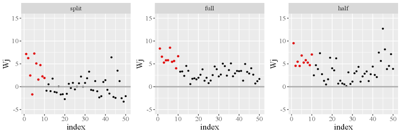
The total computational complexity of Algorithm 1 is of order O(2nHp2+plogp)O(2nHp^{2}+p\log p) so that this algorithm can be easily implemented. Practically, our method involves data splitting that may lead to some information loss concerning the full data (Du et al., 2023). Fortunately, we obtain a data-driven threshold by the marginal symmetry property of WjW_{j} under the null, which does not need to find the null asymptotic distribution anymore. Here we use a toy example to illustrate the advantage of data splitting. Further details regarding the data generation can be found in Section 5. In Figure 1, we observe that the data splitting method (left panel) places most active variables above zero, and many inactive variables are symmetrically distributed around zero. This is a crucial property for our selection procedure while the full estimation (middle panel) and half data estimation (right panel) methods both fail to achieve this level of symmetry.

Refer to caption
Figure 1: Scatterplots of WjW_{j}’s with red points and black dots denoting active and inactive variables, respectively. Left panel: the proposed WjW_{j} in (6); Middle panel: Wj=h=1H|β^hj|W_{j}=\sum\nolimits_{h=1}^{H}|\widehat{\beta}_{hj}| with (B^)hj=β^hj(\widehat{\textbf{B}})_{hj}=\widehat{\beta}_{hj}, which is the least square estimator on the full data; Right panel: replace B^2\widehat{\textbf{B}}_{2} with B^1\widehat{\textbf{B}}_{1} in (6).

3.2 High-dimensional procedure

When the dimension pp is very large in practice, the above procedure does not work since the ordinary least square procedure cannot be directly implemented. Note that our data splitting procedure can be essentially extended to the version of the regularization form. Inspired by the idea of SDA filter proposed by Du et al. (2023), we then develop the following selection procedure for high-dimensional data.

To extract information from 𝒟1\mathcal{D}_{1}, we replace the least square solution in (3) with LASSO selector (Tibshirani, 1996) as follows

𝜷^λh(1)=argmin𝜷h[n1i=1n{fh(Yi)𝐗i𝜷h}2+λh𝜷h1],h=1,,H,\displaystyle\widehat{\bm{\beta}}^{(1)}_{\lambda_{h}}=\arg\min_{\bm{\beta}_{h}}\left[n^{-1}\sum\limits_{i=1}^{n}\left\{f_{h}(Y_{i})-{\bf X}_{i}^{\top}\bm{\beta}_{h}\right\}^{2}+\lambda_{h}\|\bm{\beta}_{h}\|_{1}\right],~{}~{}h=1,\ldots,H, (8)

where λh>0\lambda_{h}>0 is a tuning parameter. It is worth noting that although the LASSO estimator does not provide guarantees on the FDR control of the selected variables, it still serves as a useful tool here that simultaneously takes into account the sparsity and dependence structures as described in Du et al. (2023). It is not necessary to penalize HH slices of coefficients simultaneously to establish 𝐁{\bf B}. This is quite different from the traditional model-free variable selection methods, such as Wu and Li (2011).

Let 𝒮={j:h=1H|β^λh,j(1)|>0}\mathcal{S}=\{j:\sum\nolimits_{h=1}^{H}|\widehat{\beta}^{(1)}_{\lambda_{h},j}|>0\} be the subset of variables selected by (8), where β^λh,j(1)\widehat{\beta}^{(1)}_{\lambda_{h},j} is the jjth element of 𝜷^λh\widehat{\bm{\beta}}_{\lambda_{h}}. We then use 𝒟2\mathcal{D}_{2} to obtain the least square estimates B^2𝒮\widehat{\textbf{B}}_{2\mathcal{S}} in (3) for coordinates in the narrowed subset 𝒮\mathcal{S}. Denote the estimates from 𝒟1\mathcal{D}_{1} and 𝒟2\mathcal{D}_{2} be 𝐁^1\widehat{\bf{B}}_{1} and 𝐁^2\widehat{\bf{B}}_{2}, where

B^2j={B^2𝒮j,j𝒮;𝟎,otherwise.\displaystyle{\widehat{\textbf{B}}}_{2j}=\begin{cases}{\widehat{\textbf{B}}}_{2\mathcal{S}j},&\quad j\in\mathcal{S};\\ \bm{0},&\quad\mbox{otherwise}.\end{cases}

Accordingly, the ranking statistics in the high-dimensional setting are constructed as

Wj=B^1jB^2js1𝒮js2𝒮j,j=1,,p,\displaystyle{W}_{j}=\frac{\widehat{\textbf{B}}_{1j}^{\top}\widehat{\textbf{B}}_{2j}}{s_{1\mathcal{S}j}s_{2\mathcal{S}j}},~{}~{}j=1,\ldots,p,

where sk𝒮j2=𝒆j(i=1n𝐗k𝒮i𝐗k𝒮i)1𝒆js_{k\mathcal{S}j}^{2}=\bm{e}_{j}^{\top}\left(\sum\nolimits_{i=1}^{n}{\bf X}_{k\mathcal{S}i}{\bf X}_{k\mathcal{S}i}^{\top}\right)^{-1}\bm{e}_{j}, k=1,2k=1,2, with narrowed subset 𝒮\mathcal{S}. The statistics Wj{W}_{j} has similar properties to the proposed one in (6), which is (asymptotically) symmetric with mean zero for j𝒜cj\in\mathcal{A}^{c} and is a large positive value for j𝒜j\in\mathcal{A} without imposing the relationship between YY and 𝐗{\bf X}. Therefore, we propose to choose a threshold L+{L}_{+}

L+=inf{t>0:1+#{j:Wjt}#{j:Wjt}1α},\displaystyle{L}_{+}=\inf\left\{t>0:\frac{1+\#\left\{j:{W}_{j}\leq-t\right\}}{\#\left\{j:{W}_{j}\geq t\right\}\vee 1}\leq\alpha\right\}, (9)

and select the active variables by 𝒜^(L+)={j:WjL+,1jp}\widehat{\mathcal{A}}({L}_{+})=\left\{j:{W}_{j}\geq{L}_{+},1\leq j\leq p\right\} in high-dimensional setting. The proposed L+{L}_{+} in (9) shares a similar spirit to Model-X Knockoff (Candes et al., 2018) or SDA filter (Du et al., 2023) to obtain an accurate FDR control. However, in the high-dimensional variable selection problems, we usually can not collect enough information on (Y,𝐗)(Y,{\bf X}), and the exact knockoff copies may not be available when p>np>n. Fortunately, MFSDS does not require any prior information on the distribution of (Y,𝐗)(Y,{\bf X}) or the asymptotic distribution of statistics, and thus it is more suitable for high-dimensional problems.

4 Theoretical results

In this section, we entirely focus on controlling FDR. We begin by imposing a mild restriction on the response transformation function f(Y)f(Y).

Assumption 1 (Response transformation).

Function f(Y)f(Y) satisfies 𝔼{f(Y)}=0\mathbb{E}\left\{f(Y)\right\}=0 and var{f(Y)𝐗𝛃0}<{\rm{var}}\left\{f(Y)-{\bf X}^{\top}\bm{\beta}_{0}\right\}<\infty.

Assumption 1 distinguishes our approach from most model-based selection methods by transforming a general model into a multivariate response linear problem, thereby achieving model-free variable selection (Wu and Li, 2011). The transformed errors are not independent of the covariates and thus we need more effort for the theoretical analysis. Our first theorem is a finite sample theory for FDR control.

Theorem 4.1 (Finite-sample FDR control).

Suppose Assumption 1 hold. Assume that the statistics WjW_{j}, 1jp1\leq j\leq p, are well-defined. For any α(0,1)\alpha\in(0,1), the FDR of our model-free selection procedure satisfies

FDRminϵ0{α(1+4ϵ)+Pr(maxj𝒜cΔj>ϵ)},\displaystyle{\rm{FDR}}\leq\min_{\epsilon\geq 0}\left\{\alpha\left(1+4\epsilon\right)+\text{Pr}\left(\max_{j\in\mathcal{A}^{c}}\Delta_{j}>\epsilon\right)\right\},

where Δj=|Pr(Wj>0|Wj|,𝐖j)1/2|\Delta_{j}=\left|{\text{Pr}}\left(W_{j}>0\mid|W_{j}|,{\bf{W}}_{-j}\right)-1/2\right| and 𝐖j=(W1,,Wp)Wj{\bf{W}}_{-j}=\left(W_{1},\ldots,W_{p}\right)^{\top}\setminus W_{j}.

Theorem 4.1 holds regardless of the unknown relationship between variables 𝐗{\bf X} and response YY. This result can be established using the techniques developed in Barber et al. (2020). The quantity Δj\Delta_{j} is interpreted as a measure to investigate the effect of both the asymmetry of WjW_{j} and the dependence between WjW_{j} and Wj\textbf{W}_{-j} on FDR. In asymmetric cases, it is still expected that Δj\Delta_{j} will be small, given that both β^hj(1)\widehat{\beta}^{(1)}_{hj} and β^hj(2)\widehat{\beta}^{(2)}_{hj} converge to normal distributions if nn is not too small. Theorem 4.1 implies that tight control of Δj\Delta_{j}’s under asymmetric cases also results in effective FDR control.

For asymptotic FDR control of the proposed procedure, we require the following technical assumptions, which are not the weakest one but facilitate the technical proofs in the Supplementary Material. Let 𝐀𝚺𝒮=Op(anp)\|{\bf A}-\bm{\Sigma}_{\mathcal{S}}\|_{\infty}=O_{p}(a_{np}) with anp0a_{np}\to 0, where 𝐀=n1i=1n𝐗2𝒮i𝐗2𝒮i{\bf A}=n^{-1}\sum\nolimits_{i=1}^{n}{\bf X}_{2\mathcal{S}i}{\bf X}_{2\mathcal{S}i}^{\top} and 𝚺𝒮=𝔼(𝐗𝒮𝐗𝒮)\bm{\Sigma}_{\mathcal{S}}={\mathbb{E}}({\bf X}_{\mathcal{S}}{\bf X}_{\mathcal{S}}^{\top}). Define υn=max{𝚺𝒮,𝚺𝒮1}\upsilon_{n}=\max\left\{\|\bm{\Sigma}_{\mathcal{S}}\|_{\infty},\|\bm{\Sigma}^{-1}_{\mathcal{S}}\|_{\infty}\right\} and B0𝒮={Bj:j𝒮}\textbf{B}_{0\mathcal{S}}=\left\{\textbf{B}_{j}:j\in\mathcal{S}\right\}. Denote dn=|𝒜|d_{n}=|\mathcal{A}|, qn=|𝒮|q_{n}=|\mathcal{S}| and q0n=|𝒮𝒜c|q_{0n}=|\mathcal{S}\cap\mathcal{A}^{c}|. Assume that qnq_{n} is uniformly bounded above by some non-random sequence q¯n\bar{q}_{n}.

Assumption 2 (Sure screening property).

As nn\to\infty, Pr(𝒜𝒮)1.\rm{Pr}(\mathcal{A}\subseteq\mathcal{S})\to 1.

Assumption 3 (Moments).

Let 𝛆=𝐟𝐁0𝒮𝐗𝒮H\bm{\varepsilon}={\bf f}-{\bf B}_{0\mathcal{S}}^{\top}{\bf X}_{\mathcal{S}}\in\mathbb{R}^{H}. Conditioning on 𝒮\mathcal{S}, there exists a positive diverging sequence KnK_{n} and a constant ϖ>2\varpi>2 such that

max1hHmax1in𝔼(𝚺𝒮1𝐗2𝒮iεihϖ)Knϖ,\displaystyle\max_{1\leq h\leq H}\max_{1\leq i\leq n}\mathbb{E}(\|\bm{\Sigma}_{\mathcal{S}}^{-1}{\bf X}_{2\mathcal{S}i}\varepsilon_{ih}\|_{\infty}^{\varpi})\leq K_{n}^{\varpi},

for i𝒟2i\in\mathcal{D}_{2}. Assume that as nn\to\infty, q¯n1/ϖ+γ+1/2Kn/n1/2γ1/ϖ0\bar{q}_{n}^{1/\varpi+\gamma+1/2}K_{n}/n^{1/2-\gamma-1/\varpi}\to 0 for some small γ>0\gamma>0.

Assumption 4 (Design matrix).

There exist positive constants κ¯\underline{\kappa} and κ¯\bar{\kappa} such that

κ¯liminfnλmin(𝐗2𝒮𝐗2𝒮/n)<limsupnλmax(𝐗2𝒮𝐗2𝒮/n)κ¯,\displaystyle\underline{\kappa}\leq\lim\inf_{n\rightarrow\infty}\lambda_{\min}({\bf X}_{2\mathcal{S}}^{\top}{\bf X}_{2\mathcal{S}}/n)<\lim\sup_{n\rightarrow\infty}\lambda_{\max}({\bf X}_{2\mathcal{S}}^{\top}{\bf X}_{2\mathcal{S}}/n)\leq\bar{\kappa},

hold with probability one.

Assumption 5 (Estimation accuracy).

Assume that 𝐁^1j𝐁j2=Op(cnp)\|\widehat{\bf B}_{1j}-{\bf B}_{j}\|_{2}=O_{p}(c_{np}) uniformly holds for j𝒮j\in\mathcal{S}, where 𝐁^1\widehat{\bf B}_{1} is an estimator of 𝐁\bf B from 𝒟1\mathcal{D}_{1} , cnp0c_{np}\to 0 and 1/(ncnp)=O(1)1/(\sqrt{n}c_{np})=O(1).

Assumption 6 (Signals).

Denote 𝒞𝐁={j𝒜:𝐁j22/max{cnp2,q¯nlogq¯n/n}}\mathcal{C}_{\bf B}=\left\{j\in\mathcal{A}:\|{\bf B}_{j}\|_{2}^{2}/\max\left\{c_{np}^{2},\bar{q}_{n}\log{\bar{q}_{n}}/n\right\}\to\infty\right\}. Let ηn:=|𝒞𝐁|\eta_{n}:=|\mathcal{C}_{\bf B}|\to\infty as (n,p)(n,p)\to\infty.

Assumption 7 (Dependence).

Let ρjl\rho_{jl} denotes the conditional correlation between WjW_{j} and WlW_{l} given 𝒟1\mathcal{D}_{1}. Assume that for each jj and some C>0C>0, #{l𝒜c:|ρjl|C(logn)2ν}rp\#\{l\in\mathcal{A}^{c}:|\rho_{jl}|\geq C(\log n)^{-2-\nu}\}\leq r_{p}, where ν>0\nu>0 is some small constant, and rp/ηn0r_{p}/\eta_{n}\to 0 as (n,p)(n,p)\to\infty.

Remark 1.

Assumption 2 has been used in Meinshausen et al. (2009); Barber and Candès (2019); Du et al. (2023) to ensure that 𝐁^2j\widehat{{\bf B}}_{2j} is unbiased for j𝒮j\in\mathcal{S}. Assumptions 3 and 4 are commonly used in the context of variable selection. The rate cnpc_{np} in Assumption 5 ensures that 𝐁^1\widehat{\bf B}_{1} is a reasonable estimator of 𝐁\bf B from 𝒟1\mathcal{D}_{1}. For the LASSO selector, cnp=dnlogp/nc_{np}=d_{n}\sqrt{\log p/n} typically satisfies the Assumption 5. Assumption 6 implies that the number of informative covariates with identifiable effect sizes is not too small as (n,p)(n,p)\to\infty. Assumption 7 allows WjW_{j} to be correlated with all others but requires that the correlation coefficients need to converge to zero at a log rate. This condition is similar to the weak dependence structure given in Fan et al. (2012).

Theorem 4.2 (Asymptotic FDR control).

Suppose Assumptions 1-7 and hold. For any α(0,1)\alpha\in(0,1), cnpanpυnnq¯n(logq¯n)3/2+γ0c_{np}a_{np}\upsilon_{n}\sqrt{n\bar{q}_{n}}(\log{\bar{q}_{n}})^{3/2+\gamma}\to 0 for a small γ>0\gamma>0, the FDP of the MFSDS procedure with threshold LL satisfies

FDP(L)\displaystyle{\rm FDP}(L) :=#{j:WjL,j𝒜c}#{j:WjL}1α+op(1),\displaystyle:=\frac{\#\{j:W_{j}\geq L,j\in\mathcal{A}^{c}\}}{\#\{j:W_{j}\geq L\}\vee 1}\leq\alpha+o_{p}(1),

and limsup(n,p)FDRα\mathop{\lim\sup}_{(n,p)\to\infty}{\rm FDR}\leq\alpha.

Theorem 4.2 implies that the variable selection procedure with the data-driven threshold LL can control the FDR at the target level asymptotically. Further investigations are needed to better understand the condition cnpanpυnnq¯n(logq¯n)3/2+γ0c_{np}a_{np}\upsilon_{n}\sqrt{n\bar{q}_{n}}(\log{\bar{q}_{n}})^{3/2+\gamma}\to 0. The conventional result of 𝐀𝚺𝒮\|{\bf A}-\bm{\Sigma}_{\mathcal{S}}\|_{\infty} indicates that anp=Op(υnlogq¯n/n)a_{np}=O_{p}(\upsilon_{n}\sqrt{\log\bar{q}_{n}/n}). With cnp=dnlogp/nc_{np}=d_{n}\sqrt{\log p/n} of LASSO selector, the condition degenerates to dnυn2q¯n/n0d_{n}\upsilon_{n}^{2}\sqrt{\bar{q}_{n}/n}\to 0 if pp is of a polynomial rate of nn. The above condition basically imposes restrictions on the rate of dnd_{n}, υn\upsilon_{n}, and q¯n\bar{q}_{n}. Accordingly, the screening stage on split 𝒟1\mathcal{D}_{1} must satisfy q¯n=o(n)\bar{q}_{n}=o(n) if we assume that dnd_{n} and υn\upsilon_{n} are bounded. Alternatively, if we only assume that υn\upsilon_{n} is bounded, then a sufficient requirement for the condition in Theorem 4.2 is q¯n=o(n1/2)\bar{q}_{n}=o(n^{1/2}) since dnq¯nd_{n}\leq\bar{q}_{n}. This is a reasonable rate in the problem with a diverging number of parameters, such as Fan and Peng (2004) and Wu and Li (2011).

5 Numerical studies

We evaluate the performance of our proposed procedure on several simulated datasets and a real-data example under low-dimensional and high-dimensional settings.

5.1 Implantation details

We compared our MFSDS with several benchmark methods. The first one is the marginal coordinate test in sliced inverse regression (SIR, Cook, 2004), which aims at controlling the error rate for each coordinate. To make a global error rate control, we then apply the BH procedure (Benjamini and Hochberg, 1995) to the pp-values. This method is implemented using functions “dr” and “drop1” in R package dr. The second method is the Model-X Knockoff (Candes et al., 2018), which also is a model-free and data-driven variable selection procedure as the proposed method. This method is implemented by the function “create.gaussian” in R package knockoff using the lasso signed maximum feature important statistics. The two methods are termed MSIR-BH and MX-Knockoff, respectively.

We set the FDR level to α=0.2\alpha=0.2 and conducted 500 replications for all simulation results. The performance of the proposed MFSDS is evaluated along with the above benchmarks through the comparisons of FDR, the true positive rate (TPR), Pa=Pr(𝒜𝒜^(L))P_{a}=\text{Pr}(\mathcal{A}\subseteq\widehat{\mathcal{A}}(L)) and the average computing time.

5.1.1 Low-dimensional studies

We generate the covariates 𝐗{\bf X} following three distributions: multivariate normal distribution 𝒩(0,𝚺)\mathcal{N}\left(0,\bm{\Sigma}\right) with 𝚺=(σij)=ρ|ij|\bm{\Sigma}=(\sigma_{ij})=\rho^{|i-j|}, 1i,jp1\leq i,j\leq p; multivariate t(5)t(5) distribution with covariance 𝚺\bm{\Sigma}; a mixed distribution which consists of {Xj}j=1[p/3]\left\{X_{j}\right\}_{j=1}^{[p/3]} are from 𝒩(0,𝚺[p/3])\mathcal{N}\left(0,\bm{\Sigma}_{[p/3]}\right), {Xj}j=[p/3]+1[2p/3]\left\{X_{j}\right\}_{j=[p/3]+1}^{[2p/3]} are from 𝒩(0,𝐈[p/3])\mathcal{N}\left(0,{\bf I}_{[p/3]}\right), and {Xj}j=[2p/3]+1p\left\{X_{j}\right\}_{j=[2p/3]+1}^{p} are i.i.d from a t(5)t(5) distribution. The error term η\eta is the standard normal distribution which is independent of 𝐗{\bf X}. We fix (p,p1)=(20,10)\left(p,p_{1}\right)=(20,10). For a scalar cc, write 𝒄p=(c,,c)\bm{c}_{p}=(c,\dots,c) be the pp-dimensional row vector of cc’s. Five models have been considered:

  • Scenario 1a: Y=𝜷𝐗+3ηY=\bm{\beta}^{\top}{\bf X}+3\eta, where 𝜷=(𝟏p1,𝟎pp1)\bm{\beta}=(\bm{1}_{p_{1}},\bm{0}_{p-p_{1}})^{\top}.

  • Scenario 1b: Y=|𝜷1𝐗|+exp(3+𝜷2𝐗)+ηY=\left|\bm{\beta}_{1}^{\top}{\bf X}\right|+\exp\left(3+\bm{\beta}_{2}^{\top}{\bf X}\right)+\eta, where 𝜷1=(𝟏5,𝟎p5)\bm{\beta}_{1}=(\bm{1}_{5},\bm{0}_{p-5})^{\top}, 𝜷2=(𝟎5,𝟏5,𝟎pp1)\bm{\beta}_{2}=(\bm{0}_{5},\bm{1}_{5},\bm{0}_{p-p_{1}})^{\top}.

  • Scenario 1c: Y=𝜷1𝐗+(𝜷2𝐗+3)2+exp(𝜷3𝐗)+ηY=\bm{\beta}_{1}^{\top}{\bf X}+\left(\bm{\beta}_{2}^{\top}{\bf X}+3\right)^{2}+\exp\left(\bm{\beta}_{3}^{\top}{\bf X}\right)+\eta, where 𝜷1=(𝟏3,𝟎p3)\bm{\beta}_{1}=(\bm{1}_{3},\bm{0}_{p-3})^{\top}, 𝜷2=(𝟎3,𝟏3,𝟎p6)\bm{\beta}_{2}=(\bm{0}_{3},\bm{1}_{3},\bm{0}_{p-6})^{\top}, 𝜷3=(𝟎6,𝟏4,𝟎pp1)\bm{\beta}_{3}=(\bm{0}_{6},\bm{1}_{4},\bm{0}_{p-p_{1}})^{\top}.

  • Scenario 1d: Y=𝜷1𝐗/{0.5+(1.5+𝜷2𝐗)2}+(𝜷3𝐗)2+exp(𝜷4𝐗)+ηY=\bm{\beta}_{1}^{\top}{\bf X}/\left\{0.5+(1.5+\bm{\beta}_{2}^{\top}{\bf X})^{2}\right\}+(\bm{\beta}_{3}^{\top}{\bf X})^{2}+\exp(\bm{\beta}_{4}^{\top}{\bf X})+\eta, where 𝜷1=(𝟏2,𝟎p2)\bm{\beta}_{1}=(\bm{1}_{2},\bm{0}_{p-2})^{\top}, 𝜷2=(𝟎2,𝟏2,𝟎p4)\bm{\beta}_{2}=(\bm{0}_{2},\bm{1}_{2},\bm{0}_{p-4})^{\top}, 𝜷3=(𝟎4,𝟏2,𝟎p6)\bm{\beta}_{3}=(\bm{0}_{4},\bm{1}_{2},\bm{0}_{p-6})^{\top}, 𝜷4=(𝟎6,𝟏4,𝟎pp1)\bm{\beta}_{4}=(\bm{0}_{6},\bm{1}_{4},\bm{0}_{p-p_{1}})^{\top}.

  • Scenario 1e: Y=2(𝜷1𝐗)2sin(𝜷2𝐗)+3(𝜷3𝐗)3exp(𝜷4𝐗)+|𝜷5𝐗|ηY=2(\bm{\beta}_{1}^{\top}{\bf X})^{2}\sin(\bm{\beta}_{2}^{\top}{\bf X})+3(\bm{\beta}_{3}^{\top}{\bf X})^{3}\exp(\bm{\beta}_{4}^{\top}{\bf X})+|{\bm{\beta}_{5}^{\top}{\bf X}}|\eta, where 𝜷1=(𝟏2,𝟎p2)\bm{\beta}_{1}=(\bm{1}_{2},\bm{0}_{p-2})^{\top}, 𝜷2=(𝟎2,𝟏2,𝟎p4)\bm{\beta}_{2}=(\bm{0}_{2},\bm{1}_{2},\bm{0}_{p-4})^{\top}, 𝜷3=(𝟎4,𝟏2,𝟎p6)\bm{\beta}_{3}=(\bm{0}_{4},\bm{1}_{2},\bm{0}_{p-6})^{\top}, 𝜷4=(𝟎6,𝟏2,𝟎p8)\bm{\beta}_{4}=(\bm{0}_{6},\bm{1}_{2},\bm{0}_{p-8})^{\top}, 𝜷5=(𝟎8,𝟏2,𝟎pp1)\bm{\beta}_{5}=(\bm{0}_{8},\bm{1}_{2},\bm{0}_{p-p_{1}})^{\top}.

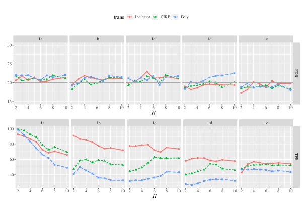
We first consider three response transformation functions fh(Y),h=1,,Hf_{h}(Y),h=1,\ldots,H, for the proposed MFSDS: (1) the slice indicator function (Li, 1991) that fh(Y)=1f_{h}(Y)=1 if YY is in the hhth slice and 0 otherwise; (2) The CIRE-type response transformation (Cook and Ni, 2006) that fh(Y)=Yf_{h}(Y)=Y if YY is in the hhth slice and 0 otherwise; (3) the normalized polynomial response transformation (Yin and Cook, 2002) that fh(Y)=Yhf_{h}(Y)=Y^{h} if YY is in the hhth slice and 0 otherwise. We name these three functions as Indicator, CIRE, and Poly, respectively.

Figure 2 shows that our proposed procedure successfully controls FDR in an acceptable range of the target level, regardless of the number of working dimension HH and the response transformation functions. The three response transformation functions exhibit similar patterns with FDR control, and we do not address which f(Y)f(Y) is the “best” in this paper. Our methodology does not require the estimation of dd with a given HH. In the rest of the simulations, we focus on the slice indicator function and fix H=4H=4 for the proposed MFSDS.

Refer to caption
Figure 2: FDR and TPR(%) of the proposed MFSDS against different HH and fh(Y)f_{h}(Y) under Scenarios 1a-1e when (n,ρ)=(500,0.5)(n,\rho)=(500,0.5) and 𝐗{\bf X} is normal distribution. The gray solid line denotes the target FDR level.

Next, we compare FDR and TPR of the proposed MFSDS under low-dimensional settings with marginal SIR and MX-Knockoff in Table 1 and Table 2. Table 1 studies how the proposed MFSDS and the benchmark methods are affected by the covariate distributions. Table 2 displays the comparisons of covariate correlation for the three methods. Across all scenarios, the FDRs of MFSDS persist at the desired level consistently and the TPRs of MFSDS are higher than MSIR-BH and MX-Knockoff in most cases. Further discussion can be found below.

  • (a)

    MFSDS vs MSIR-BH. The marginal SIR (Cook, 2004) with BH procedure (Benjamini and Hochberg, 1995) controls the FDR in all settings but can be overly conservative in some cases. This is because the BH procedure controls the FDR at level αp0/p\alpha p_{0}/p in a low-dimensional setting. By contrast, MFSDS performs accurate FDR control and better TPR in both linear and nonlinear models. It seems that the power of the proposed MFSDS is slightly lower than MSIR-BH in very few cases since MFSDS involves data splitting to construct the statistic symmetry property. But additional simulations show that, as the sample size nn increases, our method will be more effective than others in low-dimensional settings.

  • (b)

    MFSDS vs MX-Knockoff. MFSDS and MX-Knockoff are both model-free and data-driven variable selection methods. However, MX-Knockoff requires knowing the joint distribution of the covariates. The proposed MFSDS controls the FDR more accurately near the desired level, while MX-Knockoff fails to control the FDR for t(5)t(5) distribution in Column 2 of Table 1. Furthermore, Table 1 shows that MX-Knockoff works not well as our MFSDS in nonlinear cases. Table 2 indicates that the MFSDS robustly controls the FDR at the nominal level, but the MX-Knockoff exhibits more conservative FDR and lower TPR as the correlation increases across all scenarios.

Table 1: FDR and TPR (%) for three methods against different covariate distributions under Scenarios 1a-1e when (n,ρ)=(500,0.5)(n,\rho)=(500,0.5).
normal t5 mixed
Scenario Method FDR TPR FDR TPR FDR TPR
MFSDS 20.7 87.1 22.0 84.4 22.2 96.4
1a MSIR-BH 10.4 91.4 10.1 84.6 10.8 98.2
MX-Knockoff 21.0 99.9 22.4 100.0 22.8 100.0
MFSDS 21.8 85.6 19.1 70.4 21.5 89.7
1b MSIR-BH 10.0 83.1 13.1 68.3 10.5 88.9
MX-Knockoff 13.3 39.9 39.4 50.6 16.3 58.9
MFSDS 21.3 78.5 20.9 68.9 20.9 84.2
1c MSIR-BH 10.5 74.8 14.1 68.1 11.2 80.9
MX-Knockoff 13.6 46.0 38.8 52.4 19.1 82.2
MFSDS 18.6 61.9 20.0 51.9 20.0 61.9
1d MSIR-BH 10.6 57.4 14.1 48.5 11.6 56.0
MX-Knockoff 14.7 40.2 38.9 52.5 18.6 51.9
MFSDS 20.2 57.1 18.7 49.5 18.0 58.2
1e MSIR-BH 11.7 51.1 12.9 46.2 10.9 52.8
MX-Knockoff 14.5 40.0 38.8 52.6 16.0 33.4

Table 2: FDR and TPR (%) for three methods against different correlation ρ\rho under Scenarios 1a-1e when n=500n=500 and 𝐗{\bf X} is from normal distribution.
ρ=0.2\rho=0.2 ρ=0.5\rho=0.5 ρ=0.8\rho=0.8
Scenario Method FDR TPR FDR TPR FDR TPR
MFSDS 22.6 99.1 20.7 87.1 14.6 27.7
1a MSIR-BH 11.0 99.9 10.4 91.4 14.0 10.0
MX-Knockoff 22.8 100.0 21.0 99.9 20.6 95.6
MFSDS 22.9 99.5 21.8 85.6 21.6 30.2
1b MSIR-BH 11.2 99.8 10.0 83.1 12.0 16.5
MX-Knockoff 15.9 54.9 13.3 39.9 10.1 20.7
MFSDS 21.6 89.9 21.3 78.5 20.2 34.9
1c MSIR-BH 11.2 85.9 10.5 74.8 11.7 18.4
MX-Knockoff 17.5 69.3 13.6 46.0 11.1 22.6
MFSDS 18.2 64.8 18.6 61.9 20.0 40.9
1d MSIR-BH 10.2 61.6 10.6 57.4 12.5 31.2
MX-Knockoff 16.7 48.0 14.7 40.2 11.5 22.5
MFSDS 19.1 64.7 20.2 57.1 18.1 45.6
1e MSIR-BH 11.2 61.2 11.7 51.1 9.6 40.2
MX-Knockoff 17.0 38.3 14.5 40.0 10.6 25.1

5.1.2 High-dimensional studies

In high-dimensional settings, we consider the following benchmarks. The competitor MSIR-BH in low-dimension does not work in high-dimensional settings since the pp-value cannot directly be obtained. Thus, the sample-splitting method (Wasserman and Roeder, 2009), which first conducts data screening using LASSO and then applies BH to the pp-values calculated by marginal SIR (Cook, 2004). Since the commonly used Akaike information criterion such as in Du et al. (2023) causes inaccurate model deviance after slicing responses, the cross-validation criterion is conducted to choose an overfitted model in the screening stage. The second method is named as MFSDS-DB (Javanmard and Montanari, 2014), which extends the least square solution in (3) to regularized version with L1L_{1} penalty in (8) and makes a bias correction with R package selectiveInference. The MX-Knockoff is conducted by the function create.second-order in R package knockoff to approximate an accurate precision matrix in high-dimensional setting (Candes et al., 2018). The fourth one is the marginal independence SIR proposed in Yu et al. (2016a). We choose two model sizes cn/log(n)\lfloor cn/\log(n)\rfloor, c=(0.05,0.5)c=(0.05,0.5), as two simple competitors and denote them as IM-SIR1 and IM-SIR2, respectively. We consider the following models when p>np>n with signal strength aa.

  • Scenario 2a: Y=aexp(5+𝜷𝐗)+ηY=a\cdot\exp\left(5+\bm{\beta}^{\top}{\bf X}\right)+\eta, where 𝜷=(𝟏p1,𝟎pp1)\bm{\beta}=(\bm{1}_{p_{1}},\bm{0}_{p-p_{1}})^{\top}.

  • Scenario 2b: Y=a{2𝜷1𝐗+3exp(𝜷2𝐗)}+ηY=a\cdot\left\{2\bm{\beta}_{1}^{\top}{\bf X}+3\exp\left(\bm{\beta}_{2}^{\top}{\bf X}\right)\right\}+\eta, where 𝜷1=(𝟏5,𝟎p5)\bm{\beta}_{1}=(\bm{1}_{5},\bm{0}_{p-5})^{\top}, 𝜷2=(𝟎5,𝟏5,𝟎pp1)\bm{\beta}_{2}=(\bm{0}_{5},\bm{1}_{5},\bm{0}_{p-p_{1}})^{\top}.

  • Scenario 2c: Y=a{𝜷1𝐗+|𝜷2𝐗+5|+exp(𝜷3𝐗)}+ηY=a\cdot\left\{\bm{\beta}_{1}^{\top}{\bf X}+\left|\bm{\beta}_{2}^{\top}{\bf X}+5\right|+\exp\left(\bm{\beta}_{3}^{\top}{\bf X}\right)\right\}+\eta, where 𝜷1=(𝟏3,𝟎p3)\bm{\beta}_{1}=(\bm{1}_{3},\bm{0}_{p-3})^{\top}; 𝜷2=(𝟎3,𝟏3,𝟎p6)\bm{\beta}_{2}=(\bm{0}_{3},\bm{1}_{3},\bm{0}_{p-6})^{\top}; 𝜷3=(𝟎6,𝟏4,𝟎pp1)\bm{\beta}_{3}=(\bm{0}_{6},\bm{1}_{4},\bm{0}_{p-p_{1}})^{\top}.

Table 3: FDR, TPR, PaP_{a}(%) and computing time (in second) for several methods against different 𝐗{\bf X} distributions under Scenarios 2a-2c when (n,p,p1,ρ,a)=(500,1000,10,0.5,1)(n,p,p_{1},\rho,a)=(500,1000,10,0.5,1).
normal mixed
Scenario Method FDR TPR PaP_{a} time FDR TPR PaP_{a} time
MFSDS 18.3 98.7 90.2 12.9 17.5 98.3 86.6 14.1
MFSDS-DB 17.1 57.9 7.0 75.1 17.0 77.3 19.8 65.5
MSIR-BH 4.5 32.8 0.0 11.4 4.2 32.9 0.0 12.6
2a IM-SIR1 0.0 40.0 0.0 26.3 0.0 40.0 0.0 34.8
IM-SIR2 75.0 100.0 100.0 26.3 75.0 100.0 100.0 34.5
MX-Knockoff 6.5 4.3 0.0 31.8 26.4 9.2 0.0 31.6
MFSDS 17.0 94.7 62.0 12.8 17.5 94.6 58.8 14.7
MFSDS-DB 15.6 71.4 4.2 74.8 16.9 80.5 14.4 75.3
MSIR-BH 5.3 34.9 0.0 11.5 4.6 34.6 0.0 13.3
2b IM-SIR1 0.0 40.0 0.0 26.3 0.0 40.0 0.0 27.3
IM-SIR2 75.0 100.0 100.0 26.3 75.0 100.0 100.0 27.1
MX-Knockoff 10.3 11.6 0.0 31.9 29.0 19.8 0.0 31.4
MFSDS 17.9 92.7 50.6 12.4 19.2 92.8 49.8 22.8
MFSDS-DB 17.0 62.1 8.0 102.3 17.4 73.2 6.0 126.8
MSIR-BH 6.5 33.4 0.0 12.2 6.3 31.1 0.0 21.8
2c IM-SIR1 0.0 40.0 0.0 22.7 0.0 40.0 0.0 36.2
IM-SIR2 75.0 100.0 100.0 22.9 75.0 100.0 100.0 35.2
MX-Knockoff 12.1 12.2 0.0 28.4 28.8 19.1 0.0 42.0

Table 3 presents the comparison results for different covariate distributions to investigate the error rate control and detection power under high-dimensional settings. The FDRs of the proposed MFSDS are approximately controlled at the target level α\alpha with a higher power, which is consistent with our theory. A similar analysis also can be found in the Supplementary Material Table S1 with a larger sample size. Table 3 and Table S1 further demonstrate that the MFSDS is able to detect all active variables when nn is large. As we can expect, although MFSDS involves data splitting which may lose some data information, its power can still be higher since the feature screening step significantly increases the signal-to-noise ratio. Besides, our method exhibits lower computing time since we avoid constructing the asymptotic distribution for each dimension in marginal coordinate test (Cook, 2004) and generating the knockoff copies in Model-X knockoff (Candes et al., 2018). We provide further explanations below.

  • (a)

    MFSDS vs MFSDS-DB. The FDR of the MFSDS-DB method controls pretty well as the proposed MFSDS but it performs a lower power than MFSDS since MFSDS-DB uses bias correction instead of the screening stage which may not boost the signal-to-noise ratio. We know that the MFSDS-DB method is an extension of our low-dimensional procedure with a debiased lasso estimate but it needs to estimate the precision matrix which results in significantly higher computational costs.

  • (b)

    MFSDS vs MSIR-BH. MSIR-BH method is a post-selection inference with marginal statistics, which achieves a conservative FDR control compared with MFSDS. It adopts data splitting (Meinshausen et al., 2009) but they only construct the marginal test statistics on 𝒟2\mathcal{D}_{2} which suffers from a serious power loss. As pointed out by reviewers, Guo et al. (2024) provided a nice refinement of MSIR-BH without data splitting, but the decorrelating process is complicated similar to the debiasing in MFSDS-DB; additional simulation in Table S2 shows that it leads intensive computation.

  • (c)

    MFSDS vs IM-SIR. The hard thresholding IM-SIR methods can detect more active variables only when model size cn/log(n)\lfloor cn/\log(n)\rfloor is greater than p1p_{1}. Table 3 implies that the hard-thresholding method can not control the FDR, and thus their large powers are unreliable with user-specified model sizes.

  • (d)

    MFSDS vs MX-Knockoff. MX-Knockoff offers a variable selection solution without making any modeling assumptions in high-dimensional situations. One important assumption in the theoretical development of MX-Knockoff is that the joint distribution of covariates 𝐗{\bf X} should be either exactly known or should be estimated robustly. Moreover, MX-Knockoff usually considers Gaussian distribution or uses a second-order approximate construction, which may lead to some invalid FDR control and power loss. By contrast, MFSDS controls the FDR more accurately under mixed distribution. In addition, the symmetry property of MFSDS stems from sample splitting while MX-Knockoff requires variable augmentation, which results in a large amount of calculation.

Refer to caption
Figure 3: FDR and TPR (%) curves against different covariate dimension pp, signal number p1p_{1}, correlation ρ\rho, and signal strength aa under Scenario 2c when n=500n=500 and 𝐗{\bf X} is from mixed distribution. The gray solid line denotes the target FDR level.

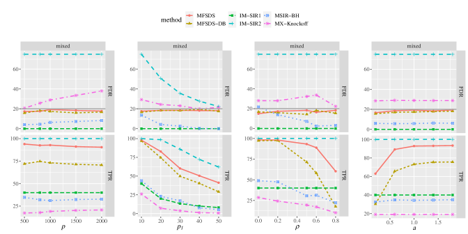
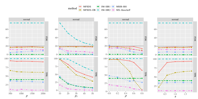
To further investigate the efficiency of our MFSDS procedure in high-dimensional settings against different covariate dimension pp, the signal number p1p_{1}, covariate correlation ρ\rho, and signal strength aa, we report the corresponding FDR and TPR in Figure 3. The FDR of MFSDS remains robust in an acceptable range of the target level no matter the dimension, signal number, correlation, and signal strength varied. Our MFSDS consistently achieves the most powerful TPR than other competitors except for IM-SIR2 since IM-SIR2 can not make a fair error rate control. The practical performance between MFSDS and MX-Knockoff is quite different. It is clear that although controlling the FDR below the target level with larger p1p_{1} in Figure 3, MX-Knockoff suffers from a larger power loss as the signal number p1p_{1} and correlation ρ\rho increases. Additional numerical results with normal covariate distribution can be found in the Supplementary Material Figure S1. Figure S1 shows that the FDR of MX-Knockoff controls quite well as MFSDS under normal distribution with various combinations pp, p1p_{1}, ρ\rho, and aa, but still a significant power gap compared to our proposed MFSDS.

5.2 Real data implementation

In this section, we apply our proposed MFSDS procedure to the children cancer data for classifying small round blue cell tumors (SRBCT), which has been analyzed by Khan et al. (2001) and Yu et al. (2016a). The SRBCT dataset aims to classify four classes of different childhood tumors sharing similar visual features during routine histology. Data were collected from 83 tumor samples and the expression measurements on 2308 genes for each sample are provided. In this dataset, we focus on investigating the performance of the FDR control between our MFSDS procedure and other existing methods.

Refer to caption
Figure 4: Scatterplots of WjW_{j}’s for MFSDS and MX-Knockoff with the red points denoting selected variables and lightblue line denoting the data-driven threshold when α=0.2\alpha=0.2.

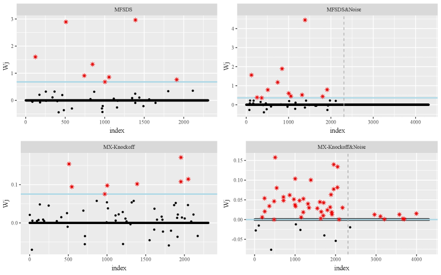
We first present the scatterplots of the ranking statistics WjW_{j}’s for MFSDS and MX-Knockoff in Figure 4. As we expect, genes with larger WjW_{j}’s are possible to be selected as influential genes (red dots), while the unselected genes (black dots) are roughly and symmetrically distributed around zero line, even though many WjW_{j}’s are exactly zero.

Table 4: Number of discovered (ND) genes and computing time (in second) in SRBCT and SRBCT&Noise datasets. Values in parentheses are the number of discovered noise variables.
SRBCT SRBCT&Noise
Method ND time ND time
MFSDS 8 1.52 12(0) 1.92
MSIR-BH 5 0.50 5(0) 0.72
IM-SIR(c=0.05) 1 130.20 1(0) 1514.23
IM-SIR(c=1) 18 128.31 18(0) 1516.59
MX-Knockoff 8 49.82 46(7) 240.20

Next, we introduce some simulated variables as inactive genes to further investigate the performance of our proposed method. Specifically, 1000 noise variables Z1Z_{1} are from 𝒩(0,1)\mathcal{N}(0,1), and another 1000 noise variables Z2Z_{2} are from t(3)t(3), which are all independently and randomly generated. We refer to this dataset as SRBCT&Noise, and our main objective is to identify the important genes from the whole 4328 variables. Since Z1Z_{1} and Z2Z_{2} are actually inactive by construction, they can be viewed as truly false discoveries. The scatterplot of WjW_{j}’s and the number of discovery genes are presented in Figure 4 and Table 4. Yu et al. Yu et al. (2016a) analyzed that an average of 9 genes out of the 2308 total genes were selected, which is very close to the number of variables selected by our method. We observed that MFSDS and MX-Knockoff identified the same number of important genes without noise variables, but MX-Knockoff mistakenly selected a small number of truly noise variables, i.e., the added noise variables. Besides, the proposed MFSDS demonstrates a relatively smaller computing time than IM-SIR and MX-Knockoff.

6 Discussion

Identifying the truly contributory variables is a critical task in statistical inference. In this paper, we proposed a novel model-free variable selection procedure with a data-driven threshold in sufficient dimension reduction framework for a family of sliced methods via data splitting. The proposed MFSDS is computationally efficient in high-dimensional settings. Theoretical and numerical results show that the proposed MFSDS can asymptotically control the FDR at the target level.

Our work raises several intriguing open questions that deserve further investigation. First, it is interesting to adopt multiple data splitting in MFSDS to improve the stability and robustness but it may require intensive computations. Equal size data splitting is used in our simulation and theory for simplicity. Second, we have checked that a larger sample size for 𝒟1\mathcal{D}_{1} will improve TPR to some extent. In addition, we sacrifice a little detection power to obtain symmetry property via data splitting, while how to construct symmetry property without data splitting or deriving complex asymptotic distribution may be another promising direction. Third, benefiting from the use of the response transformation, the proposed method can work with many classical SDR methods (such as sliced inverse regression (Li, 1991), covariance inverse regression estimator (Cook and Ni, 2006)) and many types of response (such as continuous, discrete, or categorical data). Finally, our method may also be able to dispose of the order determination problem in many situations which merits further investigation, such as Luo and Li (2016) if the importance of HH slices has been determined in advance with a diverging number of HH. It is also worth further exploring the optimal selection of working dimension HH in practice.

Appendix

This Appendix gives some key lemmas and succinct proof of theorems. We only consider the proofs under a high-dimensional setting and the low-dimensional version can be easily verified. Additional lemmas used in Appendix with their proofs and some additional simulation results can be found in the Supplementary Material.

For any vector 𝒗H{\bm{v}}\in\mathbb{R}^{H}, we have

(𝐁^2j𝐁j)𝒗\displaystyle\left(\widehat{\bf B}_{2j}-{\bf B}_{j}\right)^{\top}{\bm{v}} =𝒆j(1ni=1n𝐗2𝒮i𝐗2𝒮i)11ni=1n𝐗2𝒮i(𝐟2i𝐁0𝐗2𝒮i)𝒗\displaystyle=\bm{e}_{j}^{\top}\left(\frac{1}{n}\sum\limits_{i=1}^{n}{\bf X}_{2\mathcal{S}i}{\bf X}_{2\mathcal{S}i}^{\top}\right)^{-1}\frac{1}{n}\sum\limits_{i=1}^{n}{\bf X}_{2\mathcal{S}i}\left({\bf{f}}_{2i}-{\bf B}_{0}^{\top}{\bf X}_{2\mathcal{S}i}\right)^{\top}{\bm{v}}
=𝒆j(1ni=1n𝐗2𝒮i𝐗2𝒮i)11ni=1n𝐗2𝒮i𝜺i𝒗.\displaystyle=\bm{e}_{j}^{\top}\left(\frac{1}{n}\sum\limits_{i=1}^{n}{\bf X}_{2\mathcal{S}i}{\bf X}_{2\mathcal{S}i}^{\top}\right)^{-1}\frac{1}{n}\sum\limits_{i=1}^{n}{\bf X}_{2\mathcal{S}i}\bm{\varepsilon}_{i}^{\top}\bm{v}.

Here 𝜺=(ε1,,εH)=𝐟𝐁0𝒮𝐗𝒮H\bm{\varepsilon}=\left(\varepsilon_{1},\ldots,\varepsilon_{H}\right)^{\top}={\bf f}-{\bf B}_{0\mathcal{S}}^{\top}{\bf X}_{\mathcal{S}}\in\mathbb{R}^{H} with 𝔼(𝐗𝒮𝜺)=0\mathbb{E}({\bf X}_{\mathcal{S}}\bm{\varepsilon}^{\top})=0. However, 𝜺\bm{\varepsilon} is not independent with 𝐗𝒮{\bf X}_{\mathcal{S}} nor 𝔼(𝜺𝐗𝒮)=0\mathbb{E}\left(\bm{\varepsilon}\mid{\bf X}_{\mathcal{S}}\right)=0 due to the use of response transformation, which is quite different from the usual setting. To establish the FDR control result of our proposed procedure, we construct a modified statistic

W~j=𝐁^1j𝐁~2js1𝒮js~2𝒮j,j=1,,p,\displaystyle\widetilde{W}_{j}=\frac{\widehat{{\bf B}}_{1j}^{\top}\widetilde{{\bf B}}_{2j}}{s_{1\mathcal{S}j}\widetilde{s}_{2\mathcal{S}j}},~{}~{}j=1,\ldots,p,

where 𝐁~2j=𝒆jn1𝚺𝒮1i=1n𝐗2𝒮i𝜺2i\widetilde{\bf B}_{2j}=\bm{e}_{j}^{\top}n^{-1}\bm{\Sigma}_{\mathcal{S}}^{-1}\sum_{i=1}^{n}{\bf X}_{2\mathcal{S}i}\bm{\varepsilon}_{2i}^{\top}, s~2𝒮j2=n1𝒆j𝚺𝒮1𝒆j\widetilde{s}^{2}_{2\mathcal{S}j}=n^{-1}\bm{e}_{j}^{\top}\bm{\Sigma}_{\mathcal{S}}^{-1}\bm{e}_{j} for j𝒮j\in\mathcal{S}, and W~j=0\widetilde{W}_{j}=0 otherwise. Let G(t)=q0n1j𝒜cPr(W~jt𝒟1)G(t)={q_{0n}}^{-1}\sum_{j\in\mathcal{A}^{c}}{\Pr}(\widetilde{W}_{j}\geq t\mid\mathcal{D}_{1}), G(t)=q0n1j𝒜cPr(W~jt𝒟1)G_{-}(t)=q_{0n}^{-1}\sum_{j\in\mathcal{A}^{c}}\Pr(\widetilde{W}_{j}\leq-t\mid\mathcal{D}_{1}) and G1(y)=inf{t0:G(t)y}G^{-1}(y)=\inf\{t\geq 0:G(t)\leq y\} for 0y10\leq y\leq 1.

Before we present the proofs of the main theorems, we first state two key lemmas. The first lemma characterizes the closeness between G(t)G(t) and G(t)G_{-}(t), which plays an important role in the proof.

Lemma A.1 (Symmetry property).

Suppose Assumptions 1-4 hold. For any 0tG1(αηn/q0n)0\leq t\leq G_{-}^{-1}(\alpha\eta_{n}/{q_{0n}})

G(t)G(t)10.\displaystyle\frac{G(t)}{G_{-}(t)}-1\to 0.

The next lemma establishes the uniform convergence of j𝒜c𝕀(W~jt)/(q0nG(t)){\sum_{j\in\mathcal{A}^{c}}\mathbb{I}(\widetilde{W}_{j}\geq t)}/\left({q_{0n}G(t)}\right).

Lemma A.2 (Uniform consistency).

Suppose Assumptions 1-4 and 7 hold. Then

sup0tG1(αηn/q0n)|j𝒜c𝕀(W~jt)q0nG(t)1|\displaystyle\sup_{0\leq t\leq G^{-1}(\alpha\eta_{n}/q_{0n})}\left|\frac{\sum_{j\in\mathcal{A}^{c}}\mathbb{I}(\widetilde{W}_{j}\geq t)}{q_{0n}G(t)}-1\right| =op(1),\displaystyle=o_{p}(1), (A.1)
sup0tG1(αηn/q0n)|j𝒜c𝕀(W~jt)q0nG(t)1|\displaystyle\sup_{0\leq t\leq G_{-}^{-1}(\alpha\eta_{n}/q_{0n})}\left|\frac{\sum_{j\in\mathcal{A}^{c}}\mathbb{I}(\widetilde{W}_{j}\leq-t)}{q_{0n}G_{-}(t)}-1\right| =op(1).\displaystyle=o_{p}(1). (A.2)
Lemma A.3.

Suppose Assumptions 1-5 hold. We have

WjW~j=Op(cnpanpυnnq¯nlogq¯n).\displaystyle W_{j}-\widetilde{W}_{j}=O_{p}(c_{np}a_{np}\upsilon_{n}\sqrt{n\bar{q}_{n}\log\bar{q}_{n}}).
Lemma A.4.

Suppose Assumptions 1-5 hold with cnpanpυnnq¯n(logq¯n)3/2+γ0c_{np}a_{np}\upsilon_{n}\sqrt{n\bar{q}_{n}}(\log{\bar{q}_{n}})^{3/2+\gamma}\to 0 for a small γ>0\gamma>0. Then for any M>0M>0, we have

supMtG1(αηn/q0n)|j𝒜c𝕀(W~jt)j𝒜c𝕀(Wjt)1|=op(1),\displaystyle\sup_{M\leq t\leq G^{-1}(\alpha\eta_{n}/q_{0n})}\left|\frac{\sum_{j\in\mathcal{A}^{c}}\mathbb{I}(\widetilde{W}_{j}\geq t)}{\sum_{j\in\mathcal{A}^{c}}\mathbb{I}(W_{j}\geq t)}-1\right|=o_{p}(1),
supMtG1(αηn/q0n)|j𝒜c𝕀(W~jt)j𝒜c𝕀(Wjt)1|=op(1).\displaystyle\sup_{M\leq t\leq G_{-}^{-1}(\alpha\eta_{n}/q_{0n})}\left|\frac{\sum_{j\in\mathcal{A}^{c}}\mathbb{I}(\widetilde{W}_{j}\leq-t)}{\sum_{j\in\mathcal{A}^{c}}\mathbb{I}(W_{j}\leq-t)}-1\right|=o_{p}(1).

Proof of Theorem 4.1

We prove the finite-sample FDR control with L+L_{+}. The result for LL can be obtained similarly. The proof technique of this result has been extensively used in Barber et al. (2020) and Du et al. (2023). Fix ϵ>0\epsilon>0 and for any threshold t>0t>0, define

Rϵ(t)=j𝒜c𝕀(Wjt,Δjϵ)1+j𝒜c𝕀(Wjt).\displaystyle R_{\epsilon}(t)=\frac{\sum\nolimits_{j\in\mathcal{A}^{c}}\mathbb{I}(W_{j}\geq t,\Delta_{j}\leq\epsilon)}{1+\sum\nolimits_{j\in\mathcal{A}^{c}}\mathbb{I}(W_{j}\leq t)}.

Define an event that 𝒜={Δmaxj𝒜cΔjϵ}\mathscr{A}=\left\{\Delta\equiv\max_{j\in\mathcal{A}^{c}}\Delta_{j}\leq\epsilon\right\}. Furthermore, consider a thresholding rule L=T(𝐖)L=T(\bf{W}) that maps statistics 𝐖\bf{W} to a threshold L0L\geq 0. Define Lj=T(W1,,Wj1,|Wj|,Wj+1,,Wp)0,j=1,,p.L_{j}=T\left(W_{1},\ldots,W_{j-1},\left|W_{j}\right|,W_{j+1},\ldots,W_{p}\right)\geq 0,~{}~{}j=1,\ldots,p. Then for the proposed MFSDS with threshold L+L_{+}, we can write

j𝒜c𝕀(WjL+,Δjϵ)1j𝕀(WjL+)\displaystyle\frac{\sum\nolimits_{j\in\mathcal{A}^{c}}\mathbb{I}(W_{j}\geq L_{+},\Delta_{j}\leq\epsilon)}{1\vee\sum\nolimits_{j}\mathbb{I}(W_{j}\geq L_{+})} =1+j𝕀(WjL+)1j𝕀(WjL+)×j𝒜c𝕀(WjL+,Δjϵ)1+j𝕀(WjL+)α×Rϵ(L+).\displaystyle=\frac{1+\sum\nolimits_{j}\mathbb{I}(W_{j}\leq-L_{+})}{1\vee\sum\nolimits_{j}\mathbb{I}(W_{j}\geq L_{+})}\times\frac{\sum\nolimits_{j\in\mathcal{A}^{c}}\mathbb{I}(W_{j}\geq L_{+},\Delta_{j}\leq\epsilon)}{1+\sum\nolimits_{j}\mathbb{I}(W_{j}\leq-L_{+})}\leq\alpha\times R_{\epsilon}(L_{+}).

Next we derive an upper bound for 𝔼{Rϵ(L+)}\mathbb{E}\left\{R_{\epsilon}(L_{+})\right\}. Note that

𝔼{Rϵ(L+)}=𝔼{j𝒜c𝕀(WjL,Δjϵ)1+j𝒜c𝕀(WjL+)}=j𝒜c𝔼{𝕀(WjLj,Δjϵ)1+k𝒜c,kj𝕀(WkLj)}=j𝒜c𝔼[𝔼{𝕀(WjLj,Δjϵ)1+k𝒜c,kj𝕀(WkLj)|Wj|,𝐖j}]=j𝒜c𝔼{Pr(Wj>0|Wj|,𝐖j)𝕀(|Wj|Lj,Δjϵ)1+k𝒜c,kj𝕀(WkLj)},\displaystyle\begin{split}\mathbb{E}\left\{R_{\epsilon}(L_{+})\right\}&=\mathbb{E}\left\{\frac{\sum\nolimits_{j\in\mathcal{A}^{c}}\mathbb{I}(W_{j}\geq L,\Delta_{j}\leq\epsilon)}{1+\sum\nolimits_{j\in\mathcal{A}^{c}}\mathbb{I}(W_{j}\leq-L_{+})}\right\}\\ &=\sum\limits_{j\in\mathcal{A}^{c}}\mathbb{E}\left\{\frac{\mathbb{I}(W_{j}\geq L_{j},\Delta_{j}\leq\epsilon)}{1+\sum\nolimits_{k\in\mathcal{A}^{c},k\neq j}\mathbb{I}(W_{k}\leq-L_{j})}\right\}\\ &=\sum\limits_{j\in\mathcal{A}^{c}}\mathbb{E}\left[\mathbb{E}\left\{\frac{\mathbb{I}(W_{j}\geq L_{j},\Delta_{j}\leq\epsilon)}{1+\sum\nolimits_{k\in\mathcal{A}^{c},k\neq j}\mathbb{I}(W_{k}\leq-L_{j})}\mid\left|W_{j}\right|,{\bf{W}}_{-j}\right\}\right]\\ &=\sum\limits_{j\in\mathcal{A}^{c}}\mathbb{E}\left\{\frac{{\rm Pr}\left(W_{j}>0\mid\left|W_{j}\right|,{\bf{W}}_{-j}\right)\mathbb{I}\left(\left|W_{j}\right|\geq L_{j},\Delta_{j}\leq\epsilon\right)}{1+\sum\nolimits_{k\in\mathcal{A}^{c},k\neq j}\mathbb{I}(W_{k}\leq-L_{j})}\right\},\end{split}

where the last step holds since, after conditioning on (|Wj|,𝐖j)\left(\left|W_{j}\right|,{\bf{W}}_{-j}\right), the only unknown quantity is the sign of WjW_{j}. Recall the definition of Δj=|(Wj>0|Wj|,𝐖j)1/2|\Delta_{j}=\left|\mathbb{P}\left(W_{j}>0\mid\left|W_{j}\right|,{\bf{W}}_{-j}\right)-1/2\right|, we have (Wj>0|Wj|,𝐖j)1/2+Δj\mathbb{P}\left(W_{j}>0\mid\left|W_{j}\right|,{\bf{W}}_{-j}\right)\leq 1/2+\Delta_{j}. Thus

𝔼{Rϵ(L+)}j𝒜c𝔼{(1/2+Δj)𝕀(|Wj|Lj,Δjϵ)1+k𝒜c,kj𝕀(WkLj)}=(12+Δj)[j𝒜c𝔼{𝕀(WjLj,Δjϵ)1+k𝒜c,kj𝕀(WkLj)}+j𝒜c𝔼{𝕀(WjLj,Δjϵ)1+k𝒜c,kj𝕀(WkLj)}](12+Δj)[j𝒜c𝔼{𝕀(WjLj,Δjϵ)1+k𝒜c,kj𝕀(WkLj)}+j𝒜c𝔼{𝕀(WjLj)1+k𝒜c,kj𝕀(WkLj)}]=(12+Δj)[𝔼{Rϵ(L+)}+j𝒜c𝔼{𝕀(WjLj)1+k𝒜c,kj𝕀(WkLj)}].\displaystyle\begin{split}\mathbb{E}\left\{R_{\epsilon}(L_{+})\right\}&\leq\sum\limits_{j\in\mathcal{A}^{c}}\mathbb{E}\left\{\frac{\left(1/2+\Delta_{j}\right)\mathbb{I}\left(\left|W_{j}\right|\geq L_{j},\Delta_{j}\leq\epsilon\right)}{1+\sum\nolimits_{k\in\mathcal{A}^{c},k\neq j}\mathbb{I}(W_{k}\leq-L_{j})}\right\}\\ &=\left(\frac{1}{2}+\Delta_{j}\right)\left[\sum\limits_{j\in\mathcal{A}^{c}}\mathbb{E}\left\{\frac{\mathbb{I}\left(W_{j}\geq L_{j},\Delta_{j}\leq\epsilon\right)}{1+\sum\nolimits_{k\in\mathcal{A}^{c},k\neq j}\mathbb{I}(W_{k}\leq-L_{j})}\right\}+\sum\limits_{j\in\mathcal{A}^{c}}\mathbb{E}\left\{\frac{\mathbb{I}\left(W_{j}\leq-L_{j},\Delta_{j}\leq\epsilon\right)}{1+\sum\nolimits_{k\in\mathcal{A}^{c},k\neq j}\mathbb{I}(W_{k}\leq-L_{j})}\right\}\right]\\ &\leq\left(\frac{1}{2}+\Delta_{j}\right)\left[\sum\limits_{j\in\mathcal{A}^{c}}\mathbb{E}\left\{\frac{\mathbb{I}\left(W_{j}\geq L_{j},\Delta_{j}\leq\epsilon\right)}{1+\sum\nolimits_{k\in\mathcal{A}^{c},k\neq j}\mathbb{I}(W_{k}\leq-L_{j})}\right\}+\sum\limits_{j\in\mathcal{A}^{c}}\mathbb{E}\left\{\frac{\mathbb{I}\left(W_{j}\leq-L_{j}\right)}{1+\sum\nolimits_{k\in\mathcal{A}^{c},k\neq j}\mathbb{I}(W_{k}\leq-L_{j})}\right\}\right]\\ &=\left(\frac{1}{2}+\Delta_{j}\right)\left[\mathbb{E}\left\{R_{\epsilon}(L_{+})\right\}+\sum\limits_{j\in\mathcal{A}^{c}}\mathbb{E}\left\{\frac{\mathbb{I}\left(W_{j}\leq-L_{j}\right)}{1+\sum\nolimits_{k\in\mathcal{A}^{c},k\neq j}\mathbb{I}(W_{k}\leq-L_{j})}\right\}\right].\end{split} (A.3)

The last expression summation in (A.3) can be simplified. If for all null jj, Wj>LjW_{j}>-L_{j}, then the summation is zero. Otherwise,

j𝒜c𝔼{𝕀(WjLj)1+k𝒜c,kj𝕀(WkLj)}\displaystyle\sum\limits_{j\in\mathcal{A}^{c}}\mathbb{E}\left\{\frac{\mathbb{I}\left(W_{j}\leq-L_{j}\right)}{1+\sum\nolimits_{k\in\mathcal{A}^{c},k\neq j}\mathbb{I}(W_{k}\leq-L_{j})}\right\} =j𝒜c𝔼{𝕀(WjLj)1+k𝒜c,kj𝕀(WkLk)}=1,\displaystyle=\sum\limits_{j\in\mathcal{A}^{c}}\mathbb{E}\left\{\frac{\mathbb{I}\left(W_{j}\leq-L_{j}\right)}{1+\sum\nolimits_{k\in\mathcal{A}^{c},k\neq j}\mathbb{I}(W_{k}\leq-L_{k})}\right\}=1,

where the first equality holds by the fact: for any j,kj,k, if Wjmin(Lj,Lk)W_{j}\leq\min\left(L_{j},L_{k}\right) and Wkmin(Lj,Lk)W_{k}\leq-\min\left(L_{j},L_{k}\right), then L+j=L+kL_{+j}=L_{+k}; see Barber et al. (2020) for details.

Accordingly, we have 𝔼{Rϵ(L+)}(1/2+ϵ)[𝔼{Rϵ(L+)}+1]\mathbb{E}\left\{R_{\epsilon}(L_{+})\right\}\leq\left(1/2+\epsilon\right)\left[\mathbb{E}\left\{R_{\epsilon}(L_{+})\right\}+1\right]. As a result

𝔼{Rϵ(L+)}1/2+ϵ1/2ϵ1+4ϵ.\displaystyle\mathbb{E}\left\{R_{\epsilon}(L_{+})\right\}\leq\frac{1/2+\epsilon}{1/2-\epsilon}\leq 1+4\epsilon.

Consequently, we can naturally get the conclusions in Theorem 4.1. \hfill\square

Proof of Theorem 4.2

By the definition of FDP, our test is equivalent to select the jjth variable if WjLW_{j}\geq L, where

L=inf{t0:j𝕀(Wjt)α(1j𝕀(Wjt))}.\displaystyle L=\inf\left\{t\geq 0:\sum_{j}\mathbb{I}(W_{j}\leq-t)\leq\alpha\left(1\vee\sum_{j}\mathbb{I}(W_{j}\geq t)\right)\right\}.

We need to establish an asymptotic bound for this LL so that Lemmas A.1-A.4 can be applied. Let t=G1(αηn/q0n)t^{*}=G^{-1}_{-}(\alpha\eta_{n}/q_{0n}). By Lemmas A.2 and A.4, it follows that

αηnq0n=G(t)=1q0nj𝒜c𝕀(W~j<t){1+o(1)}=1q0nj𝒜c𝕀(Wj<t){1+o(1)},\displaystyle\frac{\alpha\eta_{n}}{q_{0n}}=G_{-}(t^{*})=\frac{1}{q_{0n}}\sum_{j\in\mathcal{A}^{c}}\mathbb{I}(\widetilde{W}_{j}<-t^{*})\{1+o(1)\}=\frac{1}{q_{0n}}\sum_{j\in\mathcal{A}^{c}}\mathbb{I}(W_{j}<-t^{*})\{1+o(1)\},

with cnpanpυnq¯nn(logq¯n)3/2+γ0c_{np}a_{np}\upsilon_{n}\bar{q}_{n}\sqrt{n}(\log{\bar{q}_{n}})^{3/2+\gamma}\to 0. On the other hand, for any j𝒞𝐁j\in\mathcal{C}_{\bf B}, where 𝒞𝐁\mathcal{C}_{\bf B} is defined in Assumption 6 and ηn=|𝒞𝐁|\eta_{n}=|\mathcal{C}_{\bf B}|, we can show that Pr(Wj<t,j𝒞𝐁)0\text{Pr}(W_{j}<t^{*},j\in\mathcal{C}_{\bf B})\to 0. In fact, it is straightforward to see that

Pr(Wj<t,for somej𝒞𝐁)\displaystyle\text{Pr}\left({W}_{j}<t^{*},\ \mbox{for some}\ j\in\mathcal{C}_{\bf B}\right)
ηnPr(𝐁^1j𝐁^2j/(s1𝒮js2𝒮j)𝐁j𝐁j/(s1𝒮js2𝒮j)<t𝐁j𝐁j/(s1𝒮js2𝒮j))\displaystyle\leq\eta_{n}\text{Pr}\left(\widehat{\bf B}_{1j}^{\top}\widehat{\bf B}_{2j}/(s_{1\mathcal{S}j}{s}_{2\mathcal{S}j})-{\bf B}_{j}^{\top}{\bf B}_{j}/(s_{1\mathcal{S}j}{s}_{2\mathcal{S}j})<t^{*}-{\bf B}_{j}^{\top}{\bf B}_{j}/(s_{1\mathcal{S}j}{s}_{2\mathcal{S}j})\right)
ηnPr(|𝐁j(𝐁^1j𝐁j+𝐁^2j𝐁j)|+|(𝐁^1j𝐁j)(𝐁^2j𝐁j)|>𝐁j𝐁jts1𝒮js2𝒮j).\displaystyle\leq\eta_{n}\text{Pr}\left(|{\bf B}_{j}^{\top}(\widehat{\bf B}_{1j}-{\bf B}_{j}+\widehat{\bf B}_{2j}-{\bf B}_{j})|+|(\widehat{\bf B}_{1j}-{\bf B}_{j})^{\top}(\widehat{\bf B}_{2j}-{\bf B}_{j})|>{\bf B}^{\top}_{j}{\bf B}_{j}-t^{*}s_{1\mathcal{S}j}{s}_{2\mathcal{S}j}\right).

Denote dj=𝐁j22ts1js2jd_{j}=\|{\bf B}_{j}\|_{2}^{2}-t^{*}s_{1j}s_{2j}. Under Assumption 6, it follows that dj=𝐁j22{1+o(1)}d_{j}=\|{\bf B}_{j}\|_{2}^{2}\{1+o(1)\}. We then get

Pr(|𝐁j(𝐁^1j𝐁j+𝐁^2j𝐁j|)+|(𝐁^1j𝐁j)(𝐁^2j𝐁j)|>dj)\displaystyle\text{Pr}\left(|{\bf B}_{j}^{\top}(\widehat{\bf B}_{1j}-{\bf B}_{j}+\widehat{\bf B}_{2j}-{\bf B}_{j}|)+|(\widehat{\bf B}_{1j}-{\bf B}_{j})^{\top}(\widehat{\bf B}_{2j}-{\bf B}_{j})|>d_{j}\right)
Pr(|𝐁j(𝐁^1j𝐁j+𝐁^2j𝐁j)|>dj/2)+Pr(|(𝐁^1j𝐁j)(𝐁^2j𝐁j)|>dj/2)\displaystyle\leq\text{Pr}\left(|{\bf B}_{j}^{\top}(\widehat{\bf B}_{1j}-{\bf B}_{j}+\widehat{\bf B}_{2j}-{\bf B}_{j})|>d_{j}/2\right)+\text{Pr}\left(|(\widehat{\bf B}_{1j}-{\bf B}_{j})^{\top}(\widehat{\bf B}_{2j}-{\bf B}_{j})|>d_{j}/2\right)
=:Λ1+Λ2.\displaystyle=:\Lambda_{1}+\Lambda_{2}.

It follows that

Λ1\displaystyle\Lambda_{1} Pr(𝐁^1j𝐁j2>dj/(4𝐁j2))+Pr(𝐁^2j𝐁j2>dj/(4𝐁j2))0,\displaystyle\leq\text{Pr}\left(\|\widehat{\bf B}_{1j}-{\bf B}_{j}\|_{2}>d_{j}/(4\|{\bf B}_{j}\|_{2})\right)+\text{Pr}\left(\|\widehat{\bf B}_{2j}-{\bf B}_{j}\|_{2}>d_{j}/(4\|{\bf B}_{j}\|_{2})\right)\to 0,
Λ2\displaystyle\Lambda_{2} Pr(𝐁^1j𝐁j2>cnp)+Pr(𝐁^2j𝐁j2>Cq¯nlogq¯n/n)0,\displaystyle\leq\text{Pr}\left(\|\widehat{\bf B}_{1j}-{\bf B}_{j}\|_{2}>c_{np}\right)+\Pr\left(\|\widehat{\bf B}_{2j}-{\bf B}_{j}\|_{2}>C\sqrt{\bar{q}_{n}\log{\bar{q}_{n}}/n}\right)\to 0,

the above result follows from Assumption 5 and the Lemma S.4 stated in Supplementary Material.

Thus, we get Pr(j𝕀(Wj>t)ηn)1\text{Pr}(\sum_{j}\mathbb{I}(W_{j}>t^{*})\geq\eta_{n})\to 1. Furthermore, we can conclude that

j𝕀(Wj<t)αηnαj𝕀(Wj>t).\displaystyle\sum_{j}\mathbb{I}(W_{j}<-t^{*})\lesssim\alpha\eta_{n}\leq\alpha\sum_{j}\mathbb{I}(W_{j}>t^{*}).

Then, we get an upper bound for LL, that is LtL\lesssim t^{*}. This implies that the proposed method can detect at least j𝕀(Wj>t)\sum\nolimits_{j}\mathbb{I}(W_{j}>t^{*}) signals.

Therefore, by Lemmas A.1, A.2 and A.4, we get

j𝒜c𝕀(WjL)j𝒜c𝕀(WjL)1𝑝0.\displaystyle\frac{\sum_{j\in\mathcal{A}^{c}}\mathbb{I}(W_{j}\geq L)}{\sum_{j\in\mathcal{A}^{c}}\mathbb{I}(W_{j}\leq-L)}-1\overset{{p}}{\longrightarrow}0. (A.4)

Write

FDP\displaystyle{\rm FDP} =j𝒜c𝕀(WjL)1j𝕀(WjL)=j𝕀(WjL)1j𝕀(WjL)×j𝒜c𝕀(WjL)j𝕀(WjL)α×R(L).\displaystyle=\frac{\sum_{j\in\mathcal{A}^{c}}\mathbb{I}\left(W_{j}\geq L\right)}{1\vee\sum_{j}\mathbb{I}(W_{j}\geq L)}=\frac{\sum_{j}\mathbb{I}\left(W_{j}\leq-L\right)}{1\vee\sum_{j}\mathbb{I}(W_{j}\geq L)}\times\frac{\sum_{j\in\mathcal{A}^{c}}\mathbb{I}\left(W_{j}\geq L\right)}{\sum_{j}\mathbb{I}\left(W_{j}\leq-L\right)}\leq\alpha\times R(L).

Note that R(L)j𝒜c𝕀(WjL)/j𝒜c𝕀(WjL)R(L)\leq{\sum_{j\in\mathcal{A}^{c}}\mathbb{I}\left(W_{j}\geq L\right)}/{\sum_{j\in\mathcal{A}^{c}}\mathbb{I}\left(W_{j}\leq-L\right)}, and thus limsupnFDPα\mathop{\lim\sup}_{n\to\infty}{\rm FDP}\leq\alpha in probability by (A.4). Thus the first assertion in Theorem 4.2 is proved.

Further, for any ϵ>0\epsilon>0, we have

FDR(1+ϵ)αR(L)+Pr(FDP(1+ϵ)αR(L)),\displaystyle{\rm{FDR}}\leq(1+\epsilon)\alpha R(L)+{\rm{Pr}}\left({\rm{FDP}}\geq(1+\epsilon)\alpha R(L)\right),

from which the second part of this theorem is proved. \Box

References

  • Barber and Candès (2015) Barber, R. F. and Candès, E. J. (2015), “Controlling the false discovery rate via knockoffs,” The Annals of Statistics, 43, 2055–2085.
  • Barber and Candès (2019) — (2019), “A knockoff filter for high-dimensional selective inference,” The Annals of Statistics, 47, 2504–2537.
  • Barber et al. (2020) Barber, R. F., Candes, E. J., and Samworth, R. J. (2020), “Robust inference with knockoffs,” The Annals of Statistics, 48, 1409–1431.
  • Benjamini and Hochberg (1995) Benjamini, Y. and Hochberg, Y. (1995), “Controlling the false discovery rate: a practical and powerful approach to multiple testing,” Journal of the Royal Statistical Society: Series B (Statistical Methodology), 57, 289–300.
  • Cai and Liu (2016) Cai, T. T. and Liu, W. (2016), “Large-scale multiple testing of correlations,” Journal of the American Statistical Association, 111, 229–240.
  • Candes et al. (2018) Candes, E., Fan, Y., Janson, L., and Lv, J. (2018), “Panning for gold: ‘model-X’ knockoffs for high dimensional controlled variable selection,” Journal of the Royal Statistical Society: Series B (Statistical Methodology), 80, 551–577.
  • Chen et al. (2010) Chen, X., Zou, C., and Cook, R. D. (2010), “Coordinate-independent sparse sufficient dimension reduction and variable selection,” The Annals of Statistics, 38, 3696–3723.
  • Cook (2004) Cook, R. D. (2004), “Testing predictor contributions in sufficient dimension reduction,” The Annals of Statistics, 32, 1062–1092.
  • Cook and Ni (2006) Cook, R. D. and Ni, L. (2006), “Using intraslice covariances for improved estimation of the central subspace in regression,” Biometrika, 93, 65–74.
  • Cook and Weisberg (1991) Cook, R. D. and Weisberg, S. (1991), “Sliced inverse regression for dimension reduction: Comment,” Journal of the American Statistical Association, 86, 328–332.
  • Dong (2021) Dong, Y. (2021), “A brief review of linear sufficient dimension reduction through optimization,” Journal of Statistical Planning and Inference, 211, 154–161.
  • Du et al. (2023) Du, L., Guo, X., Sun, W., and Zou, C. (2023), “False discovery rate control under general dependence by symmetrized data aggregation,” Journal of the American Statistical Association, 118, 607–621.
  • Fan et al. (2012) Fan, J., Han, X., and Gu, W. (2012), “Estimating false discovery proportion under arbitrary covariance dependence,” Journal of the American Statistical Association, 107, 1019–1035.
  • Fan and Li (2001) Fan, J. and Li, R. (2001), “Variable selection via nonconcave penalized likelihood and its oracle properties,” Journal of the American Statistical Association, 96, 1348–1360.
  • Fan et al. (2020) Fan, J., Li, R., Zhang, C.-H., and Zou, H. (2020), Statistical foundations of data science, CRC press.
  • Fan and Lv (2010) Fan, J. and Lv, J. (2010), “A selective overview of variable selection in high dimensional feature space,” Statistica Sinica, 20, 101–148.
  • Fan and Peng (2004) Fan, J. and Peng, H. (2004), “Nonconcave penalized likelihood with a diverging number of parameters,” The Annals of Statistics, 32, 928–961.
  • Guo et al. (2024) Guo, X., Li, R., Zhang, Z., and Zou, C. (2024), “Model-Free Statistical Inference on High-Dimensional Data,” Journal of the American Statistical Association, 1–27.
  • Javanmard and Montanari (2014) Javanmard, A. and Montanari, A. (2014), “Confidence intervals and hypothesis testing for high-dimensional regression,” The Journal of Machine Learning Research, 15, 2869–2909.
  • Khan et al. (2001) Khan, J., Wei, J. S., Ringner, M., Saal, L. H., Ladanyi, M., Westermann, F., Berthold, F., Schwab, M., Antonescu, C. R., Peterson, C., et al. (2001), “Classification and diagnostic prediction of cancers using gene expression profiling and artificial neural networks,” Nature Medicine, 7, 673–679.
  • Li and Wang (2007) Li, B. and Wang, S. (2007), “On directional regression for dimension reduction,” Journal of the American Statistical Association, 102, 997–1008.
  • Li (1991) Li, K.-C. (1991), “Sliced inverse regression for dimension reduction,” Journal of the American Statistical Association, 86, 316–327.
  • Li et al. (2005) Li, L., Dennis Cook, R., and Nachtsheim, C. J. (2005), “Model-free variable selection,” Journal of the Royal Statistical Society: Series B (Statistical Methodology), 67, 285–299.
  • Li et al. (2020) Li, L., Wen, X. M., and Yu, Z. (2020), “A selective overview of sparse sufficient dimension reduction,” Statistical Theory and Related Fields, 4, 121–133.
  • Luo and Li (2016) Luo, W. and Li, B. (2016), “Combining eigenvalues and variation of eigenvectors for order determination,” Biometrika, 103, 875–887.
  • Meinshausen et al. (2009) Meinshausen, N., Meier, L., and Bühlmann, P. (2009), “P-values for high-dimensional regression,” Journal of the American Statistical Association, 104, 1671–1681.
  • Shao et al. (2007) Shao, Y., Cook, R. D., and Weisberg, S. (2007), “Marginal tests with sliced average variance estimation,” Biometrika, 94, 285–296.
  • Svetulevičienė (1982) Svetulevičienė, V. (1982), “Multidimensional local limit theorems for probabilities of moderate deviations,” Lithuanian Mathematical Journal, 22, 416–420.
  • Tibshirani (1996) Tibshirani, R. (1996), “Regression shrinkage and selection via the lasso,” Journal of the Royal Statistical Society: Series B (Statistical Methodology), 58, 267–288.
  • Wasserman and Roeder (2009) Wasserman, L. and Roeder, K. (2009), “High dimensional variable selection,” The Annals of Statistics, 37, 2178–2201.
  • Wu and Li (2011) Wu, Y. and Li, L. (2011), “Asymptotic properties of sufficient dimension reduction with a diverging number of predictors,” Statistica Sinica, 2011, 707–703.
  • Xia et al. (2002) Xia, Y., Tong, H., Li, W., and Zhu, L.-X. (2002), “An adaptive estimation of dimension reduction space,” Journal of the Royal Statistical Society: Series B (Statistical Methodology), 64, 363–410.
  • Yin and Cook (2002) Yin, X. and Cook, R. D. (2002), “Dimension reduction for the conditional kth moment in regression,” Journal of the Royal Statistical Society: Series B (Statistical Methodology), 64, 159–175.
  • Yu and Dong (2016) Yu, Z. and Dong, Y. (2016), “Model-free coordinate test and variable selection via directional regression,” Statistica Sinica, 26, 1159–1174.
  • Yu et al. (2016a) Yu, Z., Dong, Y., and Shao, J. (2016a), “On marginal sliced inverse regression for ultrahigh dimensional model-free feature selection,” The Annals of Statistics, 44, 2594–2623.
  • Yu et al. (2016b) Yu, Z., Dong, Y., and Zhu, L.-X. (2016b), “Trace pursuit: A general framework for model-free variable selection,” Journal of the American Statistical Association, 111, 813–821.
  • Zhu (2020) Zhu, L. (2020), “Review of sparse sufficient dimension reduction: comment,” Statistical Theory and Related Fields, 4, 134–134.
  • Zou (2006) Zou, H. (2006), “The adaptive lasso and its oracle properties,” Journal of the American Statistical Association, 101, 1418–1429.

Supplementary Material for “Model-free variable selection in

sufficient dimension reduction via FDR control”

This Supplementary Material contains the proofs of some technical lemmas and additional simulation results.

S1. Additional lemmas

The first lemma is the standard Bernstein’s inequality.

Lemma S.1 (Bernstein’s inequality).

Let X1,,XnX_{1},\ldots,X_{n} be independent centered random variables a.s. bounded by A<A<\infty in absolute value. Let σ2=n1i=1n𝔼(Xi2)\sigma^{2}=n^{-1}\sum_{i=1}^{n}\mathbb{E}(X_{i}^{2}). Then for all x>0x>0,

Pr(i=1nXix)exp(x22nσ2+2Ax/3).\displaystyle{{\Pr}}\left(\sum_{i=1}^{n}X_{i}\geq x\right)\leq\exp\left(-\frac{x^{2}}{2n\sigma^{2}+2Ax/3}\right).

The second one is a moderate deviation result for the mean of random vector; See Theorem 1 in Svetulevičienė (1982).

Lemma S.2 (Moderate deviation for the independent sum).

Suppose that 𝐗1,,𝐗ns{\bf X}_{1},\ldots,{\bf X}_{n}\in\mathbb{R}^{s} are independent identically distributed random vectors with mean zero and identity covariance matrix. Let 𝔼(𝐗2q)<\mathbb{E}(\|{\bf X}\|_{2}^{q})<\infty for some q>2+c2q>2+c^{2} with c2>0c^{2}>0. Then in the domain 𝐱2clogn\|{\bf x}\|_{2}\leq c\sqrt{\log n}, one has uniformly

pn(𝐱)(2π)s/2exp(𝐱22/2)1,\displaystyle\frac{p_{n}({\bf x})}{(2\pi)^{-s/2}\exp(-\|{\bf x}\|^{2}_{2}/2)}\to 1,

as nn\to\infty. Here pn(𝐱)p_{n}({\bf x}) is the density function of i=1n𝐗i/n\sum_{i=1}^{n}{\bf X}_{i}/\sqrt{n}.

S2. Useful lemmas

For simplicity of notation, the constant cc and CC may be slightly abused hereafter. The following lemma establishes uniform bounds for 𝐁~2j\widetilde{\bf B}_{2j}, j=1,,pj=1,\ldots,p.

Lemma S.3.

Suppose Assumptions 1-4 hold. Then, for a large C>0C>0

Pr(s~2𝒮j1𝐁~2j2>σClogq¯n𝒟1)=o(1/q¯n),\displaystyle{\rm{Pr}}\left(\widetilde{s}_{2\mathcal{S}j}^{-1}\|\widetilde{\bf B}_{2j}\|_{2}>\sigma\sqrt{C\log\bar{q}_{n}}\mid\mathcal{D}_{1}\right)=o(1/\bar{q}_{n}),

holds uniformly in 𝒮𝒜c\mathcal{S}\bigcap\mathcal{A}^{c}. Here denote σ2=Hmaxh=1H𝐞j𝚺𝒮1𝔼[𝐗𝒮𝐗𝒮εh2]𝚺𝒮1𝐞j/(𝐞j𝚺𝒮1𝐞j)\sigma^{2}=H\max_{h=1}^{H}\bm{e}_{j}^{\top}\bm{\Sigma}_{\mathcal{S}}^{-1}\mathbb{E}[{\bf X}_{\mathcal{S}}{\bf X}_{\mathcal{S}}^{\top}\varepsilon_{h}^{2}]\bm{\Sigma}_{\mathcal{S}}^{-1}\bm{e}_{j}/(\bm{e}^{\top}_{j}\bm{\Sigma}_{\mathcal{S}}^{-1}\bm{e}_{j}).

  • Proof. 

    Note that

    Pr(s~2𝒮j1𝐁~2j2>x)\displaystyle{\rm{Pr}}\left(\widetilde{s}_{2\mathcal{S}j}^{-1}\|\widetilde{\bf B}_{2j}\|_{2}>x\right) =Pr(h=1H𝐁~2j,h2>x2s~2𝒮j2)\displaystyle={\rm{Pr}}\left(\sum_{h=1}^{H}\widetilde{\bf B}_{2j,h}^{2}>x^{2}\widetilde{s}_{2\mathcal{S}j}^{2}\right)
    Pr(𝐁~2j,h2>x2s~2𝒮j2/H,h=1,,H)\displaystyle\leq{\rm{Pr}}\left(\widetilde{\bf B}_{2j,h}^{2}>x^{2}\widetilde{s}_{2\mathcal{S}j}^{2}/H,\,\,\,\exists\,\,h=1,\ldots,H\right)
    HmaxhPr(|𝐁~2j,h|>xs~2j/H).\displaystyle\leq H\max_{h}{\rm{Pr}}\left(|\widetilde{\bf B}_{2j,h}|>x\widetilde{s}_{2j}/\sqrt{H}\right).

    Recall that 𝐁~2j,h=𝒆j𝚺𝒮1n1i=1n𝐗2𝒮iεih\widetilde{\bf B}_{2j,h}=\bm{e}_{j}^{\top}\bm{\Sigma}_{\mathcal{S}}^{-1}{n}^{-1}\sum_{i=1}^{n}{\bf X}_{2\mathcal{S}i}\varepsilon_{ih}. Let ={max1hHmax1in𝚺𝒮1𝐗2𝒮iεihmn}\mathcal{B}=\{\max_{1\leq h\leq H}\max_{1\leq i\leq n}\|\bm{\Sigma}_{\mathcal{S}}^{-1}{\bf X}_{2\mathcal{S}i}\varepsilon_{ih}\|_{\infty}\leq m_{n}\}, where mn=(nq¯n)1/ϖ+γKnm_{n}=(n\bar{q}_{n})^{1/\varpi+\gamma}K_{n} for some small γ>0\gamma>0. In what follows, we first work on the case of the occurrence of \mathcal{B}. Denote σh2=𝒆j𝚺𝒮1𝔼[𝐗𝒮𝐗𝒮εh2]𝚺𝒮1𝒆j\sigma^{2}_{h}=\bm{e}_{j}^{\top}\bm{\Sigma}_{\mathcal{S}}^{-1}\mathbb{E}[{\bf X}_{\mathcal{S}}{\bf X}_{\mathcal{S}}^{\top}\varepsilon_{h}^{2}]\bm{\Sigma}_{\mathcal{S}}^{-1}\bm{e}_{j} and σ2=maxhσh2H/(𝒆j𝚺𝒮1𝒆j)\sigma^{2}=\max_{h}\sigma^{2}_{h}H/(\bm{e}^{\top}_{j}\bm{\Sigma}_{\mathcal{S}}^{-1}\bm{e}_{j}). The Bernstein’s inequality in Lemma S.1 yields that

    Pr(|𝐁~2j,h|>xs~2𝒮j/Hfor somej𝒟1)\displaystyle{\rm Pr}\left(|\widetilde{\bf B}_{2j,h}|>x\widetilde{s}_{2\mathcal{S}j}/\sqrt{H}\ \ \mbox{for some}\ j\mid\mathcal{D}_{1}\right) qnmaxj𝒮Pr(|i=1n𝒆j𝚺𝒮1𝐗2𝒮iεih|>nxs~2𝒮j/H𝒟1)\displaystyle\leq q_{n}\max_{j\in\mathcal{S}}{\rm Pr}\left(\left|\sum_{i=1}^{n}\bm{e}_{j}^{\top}\bm{\Sigma}_{\mathcal{S}}^{-1}{\bf X}_{2\mathcal{S}i}\varepsilon_{ih}\right|>nx\tilde{s}_{2\mathcal{S}j}/\sqrt{H}\mid\mathcal{D}_{1}\right)
    2q¯nmaxj𝒮exp{n2x2s~2𝒮j2/H2nσh2+2nxs~2𝒮j/Hmn/3}\displaystyle\leq 2\bar{q}_{n}\max_{j\in\mathcal{S}}\exp\left\{-\frac{n^{2}x^{2}\tilde{s}^{2}_{2\mathcal{S}j}/H}{2n\sigma^{2}_{h}+2nx\tilde{s}_{2\mathcal{S}j}/\sqrt{H}\cdot m_{n}/3}\right\}
    2q¯nmaxj𝒮exp{x2𝒆j𝚺𝒮1𝒆j/H2σh2+2x𝒆j𝚺𝒮1𝒆j/nHmn/3}\displaystyle\leq 2\bar{q}_{n}\max_{j\in\mathcal{S}}\exp\left\{-\frac{x^{2}\bm{e}^{\top}_{j}\bm{\Sigma}_{\mathcal{S}}^{-1}\bm{e}_{j}/H}{2\sigma^{2}_{h}+2x\sqrt{\bm{e}^{\top}_{j}\bm{\Sigma}_{\mathcal{S}}^{-1}\bm{e}_{j}/nH}\cdot m_{n}/3}\right\}
    =2q¯nmaxj𝒮exp{x22σ2+2mnx/(3n)H/𝒆j𝚺𝒮1𝒆j}\displaystyle=2\bar{q}_{n}\max_{j\in\mathcal{S}}\exp\left\{-\frac{x^{2}}{2\sigma^{2}+2m_{n}x/(3\sqrt{n})\sqrt{H/\bm{e}_{j}^{\top}\bm{\Sigma}_{\mathcal{S}}^{-1}\bm{e}_{j}}}\right\}
    =o(1/q¯n),\displaystyle=o(1/\bar{q}_{n}),

    holds uniformly in 𝒮\mathcal{S}. here we use the condition mnlogq¯n/n=o(1)m_{n}\sqrt{\log\bar{q}_{n}/n}=o(1) which is implied by Assumption 3 and x=Clogq¯nx=\sqrt{C\log\bar{q}_{n}}. Next, we turn to consider the case on c\mathcal{B}^{c}. By Assumption 3 and Markov’s inequality

    Pr(c)nHmaxi,hPr(𝚺1𝐗2𝒮iεihϖ>mnϖ)=o(1/q¯n).\displaystyle{\rm Pr}(\mathcal{B}^{c})\leq nH\max_{i,h}{\rm Pr}(\|\bm{\Sigma}^{-1}{\bf X}_{2\mathcal{S}i}\varepsilon_{ih}\|_{\infty}^{\varpi}>m_{n}^{\varpi})=o(1/\bar{q}_{n}).

    The lemma is proved. \Box

The next lemma establishes uniform bounds for 𝐁^2j\widehat{\bf B}_{2j}, j=1,,pj=1,\ldots,p.

Lemma S.4.

Suppose Assumptions 1-4 hold. Then, for a large C>0C>0

Pr(s2𝒮j1𝐁^2j𝐁j2>σCq¯nlogq¯n𝒟1)=o(1/q¯n),\displaystyle{\rm Pr}\left(s_{2\mathcal{S}j}^{-1}\|\widehat{\bf B}_{2j}-{\bf B}_{j}\|_{2}>\sigma\sqrt{C\bar{q}_{n}\log\bar{q}_{n}}\mid\mathcal{D}_{1}\right)=o(1/{\bar{q}_{n}}),

uniformly holds for j𝒮j\in\mathcal{S}.

  • Proof. 

    By the similar proof of Lemma S.3 and Assumption 4, we have

    Pr(s2𝒮j1𝐁^2j𝐁j2>x)\displaystyle{\rm{Pr}}\left(s_{2\mathcal{S}j}^{-1}\|\widehat{\bf B}_{2j}-{\bf B}_{j}\|_{2}>x\right) HmaxhPr(|𝐁^2j,h𝐁j,h|>xs2𝒮j/H)\displaystyle\leq H\max_{h}{\rm{Pr}}\left(|\widehat{\bf B}_{2j,h}-{\bf B}_{j,h}|>xs_{2\mathcal{S}j}/\sqrt{H}\right)
    HmaxhPr(|𝐁^2j,h𝐁j,h|>x/nκ¯H).\displaystyle\leq H\max_{h}{\rm{Pr}}\left(|\widehat{\bf B}_{2j,h}-{\bf B}_{j,h}|>x/\sqrt{n\bar{\kappa}H}\right).

    Conditionally on 𝒟1\mathcal{D}_{1}, we know that 𝐁^2j,h𝐁j,h=𝒆j(n1i=1n𝐗2𝒮i𝐗2𝒮i)1n1i=1n𝐗2𝒮iεih.\widehat{\bf B}_{2j,h}-{\bf B}_{j,h}=\bm{e}_{j}^{\top}\left({n}^{-1}\sum_{i=1}^{n}{\bf X}_{2\mathcal{S}i}{\bf X}_{2\mathcal{S}i}^{\top}\right)^{-1}{n}^{-1}\sum_{i=1}^{n}{\bf X}_{2\mathcal{S}i}\varepsilon_{ih}. Using Assumption 4

    maxj𝒮|𝐁^2j,h𝐁j,h|κ¯1|1ni=1n𝒆j𝐗2𝒮iεih|κ¯1q¯nmaxj𝒮|ζj|,\displaystyle\max_{j\in\mathcal{S}}|\widehat{\bf B}_{2j,h}-{\bf B}_{j,h}|\leq\underline{\kappa}^{-1}\left|\frac{1}{n}\sum_{i=1}^{n}\bm{e}_{j}^{\top}{\bf X}_{2\mathcal{S}i}\varepsilon_{ih}\right|\leq\underline{\kappa}^{-1}\sqrt{\bar{q}_{n}}\max_{j\in\mathcal{S}}|\zeta_{j}|,

    where 𝜻=n1i=1n𝒆j𝐗2𝒮iεih\bm{\zeta}=n^{-1}\sum_{i=1}^{n}\bm{e}_{j}^{\top}{\bf X}_{2\mathcal{S}i}\varepsilon_{ih}. Let z=clogq¯n/nz=c\sqrt{\log{\bar{q}_{n}}/n} with cc being very large and LL is a positive constant. By Lemma S.1 again, we have

    Pr(maxj𝒮|ζj|>z)\displaystyle{\rm{Pr}}\left(\max_{j\in\mathcal{S}}|\zeta_{j}|>z\right) q¯nmaxj𝒮Pr(|i=1n𝒆j𝐗2𝒮iεih|>nz)\displaystyle\leq\bar{q}_{n}\max_{j\in\mathcal{S}}{\rm{Pr}}\left(\left|\sum\limits_{i=1}^{n}\bm{e}_{j}^{\top}{\bf X}_{2\mathcal{S}i}\varepsilon_{ih}\right|>nz\right)
    2q¯nmaxj𝒮exp{n2z22n𝔼[(𝒆j𝐗2𝒮i)2εih2]+2(max1hH,1in|𝒆j𝐗2𝒮iεih|)×nz/3}0,\displaystyle\leq 2{\bar{q}_{n}}\max_{j\in\mathcal{S}}\exp\left\{-\frac{n^{2}z^{2}}{2n\mathbb{E}[(\bm{e}_{j}^{\top}{\bf X}_{2\mathcal{S}i})^{2}\varepsilon_{ih}^{2}]+2(\max\nolimits_{1\leq h\leq H,1\leq i\leq n}|\bm{e}_{j}^{\top}{\bf X}_{2\mathcal{S}i}\varepsilon_{ih}|)\times nz/3}\right\}\to 0,

    where we use the condition max1hH,1in𝔼𝐗2𝒮iεihϖLKnϖ\max\nolimits_{1\leq h\leq H,1\leq i\leq n}{\mathbb{E}}\|{\bf X}_{2\mathcal{S}i}\varepsilon_{ih}\|_{\infty}^{\varpi}\leq LK_{n}^{\varpi} and (nq¯n)1/ϖ+γ×logq¯n/n0(n\bar{q}_{n})^{1/\varpi+\gamma}\times\sqrt{\log\bar{q}_{n}/n}\rightarrow 0 implied by Assumption 3. Thus, for some large C>0C>0, we have

    Pr(s2𝒮j1𝐁^2j𝐁j2>x)\displaystyle{\rm{Pr}}\left(s_{2\mathcal{S}j}^{-1}\|\widehat{\bf B}_{2j}-{\bf B}_{j}\|_{2}>x\right) HmaxhPr(|𝐁~2j,h𝐁j,h|>x/(κ¯nH))\displaystyle\leq H\max_{h}{\rm{Pr}}\left(|\widetilde{\bf B}_{2j,h}-{\bf B}_{j,h}|>x/(\bar{\kappa}\sqrt{nH})\right)
    HmaxhPr(maxj𝒮|1ni=1n𝒆j𝐗2𝒮iεih|>xκ¯/(κ¯nq¯nH))\displaystyle\leq H\max_{h}{\rm{Pr}}\left(\max_{j\in\mathcal{S}}\left|\frac{1}{n}\sum_{i=1}^{n}\bm{e}_{j}^{\top}{\bf X}_{2\mathcal{S}i}\varepsilon_{ih}\right|>x\underline{\kappa}/(\bar{\kappa}\sqrt{n\bar{q}_{n}H})\right)
    =HmaxhPr(maxj𝒮|ζj|>z)0,\displaystyle=H\max_{h}{\rm{Pr}}\left(\max_{j\in\mathcal{S}}|\zeta_{j}|>z\right)\to 0,

    hold if x=Cq¯nlogq¯nx=C\sqrt{\bar{q}_{n}\log{\bar{q}_{n}}}. \Box

S3. Proofs of lemmas in Appendix


Proof of Lemma A.1.

Define bn=σClogq¯nb_{n}=\sigma\sqrt{C\log\bar{q}_{n}} where C>0C>0. Hereafter for simplicity, we denote T1j=𝐁^1j/s1𝒮jT_{1j}=\widehat{\bf B}_{1j}/s_{1\mathcal{S}j} and T2j=𝐁~2j/s~2𝒮jT_{2j}=\widetilde{\bf B}_{2j}/\widetilde{s}_{2\mathcal{S}j}. Thus W~j=T1jT2j\widetilde{W}_{j}=T_{1j}^{\top}T_{2j}. We observe that

G(t)G(t)1=\displaystyle\frac{G(t)}{G_{-}(t)}-1= j𝒜c{Pr(W~jt𝒟1)Pr(W~jt𝒟1)}j𝒜cPr(W~jt𝒟1)\displaystyle\frac{\sum\nolimits_{j\in\mathcal{A}^{c}}\left\{\text{Pr}(\widetilde{W}_{j}\geq t\mid\mathcal{D}_{1})-\text{Pr}(\widetilde{W}_{j}\leq-t\mid\mathcal{D}_{1})\right\}}{\sum\nolimits_{j\in\mathcal{A}^{c}}\text{Pr}(\widetilde{W}_{j}\leq-t\mid\mathcal{D}_{1})}
=\displaystyle= j𝒜c{Pr(T1jT2jt,T2j2bn𝒟1)Pr(T1jT2jt,T2j2bn𝒟1)}q0nG(t)\displaystyle\frac{\sum_{j\in\mathcal{A}^{c}}\left\{\text{Pr}(T_{1j}^{\top}T_{2j}\geq t,\|T_{2j}\|_{2}\leq b_{n}\mid\mathcal{D}_{1})-\text{Pr}(T_{1j}^{\top}T_{2j}\leq-t,\|T_{2j}\|_{2}\leq b_{n}\mid\mathcal{D}_{1})\right\}}{q_{0n}G_{-}({t})}
+j𝒜c{Pr(T1jT2jt,T2j2>bn𝒟1)Pr(T1jT2jt,T2j2>bn𝒟1)}q0nG(t)\displaystyle+\frac{\sum_{j\in\mathcal{A}^{c}}\left\{\text{Pr}(T_{1j}^{\top}T_{2j}\geq t,\|T_{2j}\|_{2}>b_{n}\mid\mathcal{D}_{1})-\text{Pr}(T_{1j}^{\top}T_{2j}\leq-t,\|T_{2j}\|_{2}>b_{n}\mid\mathcal{D}_{1})\right\}}{q_{0n}G_{-}({t})}
:=\displaystyle:= Λ1+Λ2.\displaystyle\Lambda_{1}+\Lambda_{2}.

Note that G(t)G_{-}(t) is a decreasing function by definition. Firstly, for the term Λ2\Lambda_{2}, by Lemma S.3, we have

j𝒜cPr(T1jT2jt,T2j2>bn𝒟1)q0nG(t)j𝒜cPr(T2j2>bn𝒟1)αηnq¯n×o(1/q¯n)ηn,\displaystyle\frac{\sum_{j\in\mathcal{A}^{c}}\text{Pr}(T_{1j}^{\top}T_{2j}\geq t,\|T_{2j}\|_{2}>b_{n}\mid\mathcal{D}_{1})}{q_{0n}G_{-}({t})}\leq\frac{\sum_{j\in\mathcal{A}^{c}}\text{Pr}(\|T_{2j}\|_{2}>b_{n}\mid\mathcal{D}_{1})}{\alpha\eta_{n}}\lesssim\frac{\bar{q}_{n}\times o(1/\bar{q}_{n})}{\eta_{n}},

which implies Λ2=o(1)\Lambda_{2}=o(1). Recall that T2j=𝒆j𝚺𝒮1i=1n𝐗2𝒮i𝜺2i/n𝒆j𝚺𝒮1𝒆jT_{2j}^{\top}={\bm{e}_{j}^{\top}\bm{\Sigma}_{\mathcal{S}}^{-1}\sum_{i=1}^{n}{\bf X}_{2\mathcal{S}i}\bm{\varepsilon}_{2i}^{\top}}/{\sqrt{n\bm{e}_{j}\bm{\Sigma}_{\mathcal{S}}^{-1}\bm{e}_{j}}}. By Lemma S.2 and Assumption 3, we obtain that

Pr(T1jT2jt,T2j2bn𝒟1)Pr(T1jUjt,Uj2bn𝒟1)1,\displaystyle\frac{\text{Pr}(T_{1j}^{\top}T_{2j}\geq t,\|T_{2j}\|_{2}\leq b_{n}\mid\mathcal{D}_{1})}{\text{Pr}(T_{1j}^{\top}U_{j}\geq t,\|U_{j}\|_{2}\leq b_{n}\mid\mathcal{D}_{1})}\to 1,

where UjNH(0,𝚺~j)U_{j}\sim N_{H}(0,\widetilde{\bm{\Sigma}}_{j}). Here σ~lh=𝒆j𝚺𝒮1𝔼[𝜺l𝐗𝒮𝐗𝒮𝜺h]𝚺𝒮1𝒆j/𝒆j𝚺𝒮1𝒆j\widetilde{\sigma}_{lh}=\bm{e}_{j}^{\top}\bm{\Sigma}_{\mathcal{S}}^{-1}\mathbb{E}[\bm{\varepsilon}_{l}{\bf X}_{\mathcal{S}}^{\top}{\bf X}_{\mathcal{S}}\bm{\varepsilon}_{h}^{\top}]\bm{\Sigma}_{\mathcal{S}}^{-1}\bm{e}_{j}/\bm{e}_{j}^{\top}\bm{\Sigma}_{\mathcal{S}}^{-1}\bm{e}_{j} and 𝚺~j=(σ~lh)l,h=1H\widetilde{\bm{\Sigma}}_{j}=(\widetilde{\sigma}_{lh})_{l,h=1}^{H}. Similarly we get

Pr(T1jT2jt,T2j2bn𝒟1)Pr(T1jUjt,Uj2bn𝒟1)1.\displaystyle\frac{\text{Pr}(T_{1j}^{\top}T_{2j}\leq-t,\|T_{2j}\|_{2}\leq b_{n}\mid\mathcal{D}_{1})}{\text{Pr}(T_{1j}^{\top}U_{j}\leq-t,\|U_{j}\|_{2}\leq b_{n}\mid\mathcal{D}_{1})}\to 1.

Note that Pr(T1jUjt,Uj2bn𝒟1)=Pr(T1jUjt,Uj2bn𝒟1){\Pr}(T_{1j}^{\top}U_{j}\leq-t,\|U_{j}\|_{2}\leq b_{n}\mid\mathcal{D}_{1})=\Pr(T_{1j}^{\top}U_{j}\geq t,\|U_{j}\|_{2}\leq b_{n}\mid\mathcal{D}_{1}), from which we get Λ1=o(1)\Lambda_{1}=o(1) and accordingly we can claim the assertion. \Box


Proof of Lemma A.2.

We prove the first formula and the second one can be deduced similarly. By the proof of Lemma A.1, it suffices to show that

G(t)=1q0nj𝒜cPr(W~jt,T2j2bn𝒟1){1+o(1)}:=G¯(t){1+o(1)}.\displaystyle G(t)=\frac{1}{q_{0n}}\sum\limits_{j\in\mathcal{A}^{c}}{\text{Pr}}(\widetilde{W}_{j}\geq t,\|T_{2j}\|_{2}\leq b_{n}\mid\mathcal{D}_{1})\left\{1+o(1)\right\}:=\bar{G}(t)\left\{1+o(1)\right\}.

Accordingly

1q0nj𝒜c𝕀(W~jt)=1q0nj𝒜c𝕀(W~jt,T2j2bn){1+op(1)}.\displaystyle\frac{1}{q_{0n}}\sum\limits_{j\in\mathcal{A}^{c}}\mathbb{I}(\widetilde{W}_{j}\geq t)=\frac{1}{q_{0n}}\sum\limits_{j\in\mathcal{A}^{c}}\mathbb{I}(\widetilde{W}_{j}\geq t,\|T_{2j}\|_{2}\leq b_{n})\left\{1+o_{p}(1)\right\}.

Thus, we need to show the following assertion

sup0tG1(αηn/q0n)|j𝒜c𝕀(W~jt,T2j2bn)q0nG¯(t)1|\displaystyle\sup_{0\leq t\leq G^{-1}(\alpha\eta_{n}/q_{0n})}\left|\frac{\sum_{j\in\mathcal{A}^{c}}\mathbb{I}(\widetilde{W}_{j}\geq t,\|T_{2j}\|_{2}\leq b_{n})}{q_{0n}\bar{G}(t)}-1\right| =op(1).\displaystyle=o_{p}(1).

Note that the G¯(t)\bar{G}(t) is a decreasing and continuous function. Let ap=αηna_{p}=\alpha\eta_{n},z0<z1<<zhn1z_{0}<z_{1}<\cdots<z_{h_{n}}\leq 1 and ti=G¯1(zi)t_{i}=\bar{G}^{-1}(z_{i}), where z0=ap/q0n,zi=ap/q0n+bpexp(iζ)/q0n,hn={log((q0nap)/bp)}1/ζz_{0}=a_{p}/q_{0n},z_{i}=a_{p}/q_{0n}+b_{p}\exp(i^{\zeta})/q_{0n},h_{n}=\{\log((q_{0n}-a_{p})/b_{p})\}^{1/\zeta} with bp/ap0b_{p}/a_{p}\to 0 and 0<ζ<10<\zeta<1. Note that G¯(ti)/G¯(ti+1)=1+o(1)\bar{G}(t_{i})/\bar{G}(t_{i+1})=1+o(1) uniformly in ii. It is therefore enough to derive the convergence rate of the following formula

Dn=sup0ihn|j𝒜c{𝕀(W~jti,T2j2bn)Pr(W~jti,T2j2bn𝒟1)}q0nG¯(ti)|.\displaystyle D_{n}=\sup_{0\leq i\leq h_{n}}\left|\frac{\sum_{j\in\mathcal{A}^{c}}\left\{\mathbb{I}(\widetilde{W}_{j}\geq t_{i},\|T_{2j}\|_{2}\leq b_{n})-\text{Pr}(\widetilde{W}_{j}\geq t_{i},\|T_{2j}\|_{2}\leq b_{n}\mid\mathcal{D}_{1})\right\}}{q_{0n}\bar{G}(t_{i})}\right|.

Define ={T2j2bn,j𝒜c}\mathcal{B}=\left\{\|T_{2j}\|_{2}\leq b_{n},j\in\mathcal{A}^{c}\right\} and then we have

D(t)\displaystyle D(t) =𝔼[(j𝒜c{𝕀(W~j>t,T2j2bn)Pr(W~j>t,T2j2bn𝒟1)})2𝒟1]\displaystyle=\mathbb{E}\left[\left(\sum_{j\in\mathcal{A}^{c}}\left\{\mathbb{I}(\widetilde{W}_{j}>t,\|T_{2j}\|_{2}\leq b_{n})-{\Pr}(\widetilde{W}_{j}>t,\|T_{2j}\|_{2}\leq b_{n}\mid\mathcal{D}_{1})\right\}\right)^{2}\mid\mathcal{D}_{1}\right]
=j𝒜cl𝒜c{Pr(W~j>t,W~l>t𝒟1,)Pr(W~j>t𝒟1,)Pr(W~l>t𝒟1,)}{1+o(1)}.\displaystyle=\sum_{j\in\mathcal{A}^{c}}\sum_{l\in\mathcal{A}^{c}}\left\{{\Pr}(\widetilde{W}_{j}>t,\widetilde{W}_{l}>t\mid\mathcal{D}_{1},\mathcal{B})-\Pr(\widetilde{W}_{j}>t\mid\mathcal{D}_{1},\mathcal{B})\Pr(\widetilde{W}_{l}>t\mid\mathcal{D}_{1},\mathcal{B})\right\}\left\{1+o(1)\right\}.

Further define j={l𝒜c:|ρjl|C(logn)2ν}\mathcal{M}_{j}=\{l\in\mathcal{A}^{c}:|\rho_{jl}|\geq C(\log n)^{-2-\nu}\}. Here ρjl\rho_{jl} denotes the conditional correlation between W~j\widetilde{W}_{j} and W~l\widetilde{W}_{l} given 𝒟1\mathcal{D}_{1}. Recall thatW~j=𝒆j𝚺𝒮1i=1n𝐗2𝒮i𝜺2iT1j/n𝒆j𝚺𝒮1𝒆j.\widetilde{W}_{j}={\bm{e}_{j}^{\top}\bm{\Sigma}_{\mathcal{S}}^{-1}\sum_{i=1}^{n}{\bf X}_{2\mathcal{S}i}\bm{\varepsilon}_{2i}^{\top}T_{1j}}/{\sqrt{n\bm{e}_{j}^{\top}\bm{\Sigma}_{\mathcal{S}}^{-1}\bm{e}_{j}}}. It follows that

var(W~j𝒟1)\displaystyle\text{var}(\widetilde{W}_{j}\mid\mathcal{D}_{1}) =𝒆j𝚺𝒮1𝔼[𝐗𝒮𝐗𝒮(𝜺T1j)2]𝚺𝒮1𝒆j𝒆j𝚺𝒮1𝒆j,cov(W~j,W~l𝒟1)=𝒆j𝚺𝒮1𝔼[𝐗𝒮𝐗𝒮𝜺T1jT1l𝜺]𝚺𝒮1𝒆l𝒆j𝚺𝒮1𝒆j𝒆l𝚺𝒮1𝒆l.\displaystyle=\frac{\bm{e}_{j}^{\top}\bm{\Sigma}_{\mathcal{S}}^{-1}\mathbb{E}[{\bf X}_{\mathcal{S}}{\bf X}_{\mathcal{S}}^{\top}(\bm{\varepsilon}^{\top}T_{1j})^{2}]\bm{\Sigma}_{\mathcal{S}}^{-1}\bm{e}_{j}}{\bm{e}_{j}^{\top}\bm{\Sigma}_{\mathcal{S}}^{-1}\bm{e}_{j}},~{}~{}\text{cov}(\widetilde{W}_{j},\widetilde{W}_{l}\mid\mathcal{D}_{1})=\frac{\bm{e}_{j}^{\top}\bm{\Sigma}_{\mathcal{S}}^{-1}\mathbb{E}[{\bf X}_{\mathcal{S}}{\bf X}_{\mathcal{S}}^{\top}\bm{\varepsilon}^{\top}T_{1j}T_{1l}^{\top}\bm{\varepsilon}]\bm{\Sigma}_{\mathcal{S}}^{-1}\bm{e}_{l}}{\sqrt{\bm{e}_{j}^{\top}\bm{\Sigma}_{\mathcal{S}}^{-1}\bm{e}_{j}}\cdot\sqrt{\bm{e}_{l}^{\top}\bm{\Sigma}_{\mathcal{S}}^{-1}\bm{e}_{l}}}.

So we get

ρjl=𝒆j𝚺𝒮1𝔼[𝐗𝒮𝐗𝒮𝜺T1jT1l𝜺]𝚺𝒮1𝒆l𝒆j𝚺𝒮1𝔼[𝐗𝒮𝐗𝒮(𝜺T1j)2]𝚺𝒮1𝒆j𝒆l𝚺𝒮1𝔼[𝐗𝒮𝐗𝒮(𝜺T1l)2]𝚺𝒮1𝒆l.\displaystyle\rho_{jl}=\frac{\bm{e}_{j}^{\top}\bm{\Sigma}_{\mathcal{S}}^{-1}\mathbb{E}[{\bf X}_{\mathcal{S}}{\bf X}_{\mathcal{S}}^{\top}\bm{\varepsilon}^{\top}T_{1j}T_{1l}^{\top}\bm{\varepsilon}]\bm{\Sigma}_{\mathcal{S}}^{-1}\bm{e}_{l}}{\sqrt{\bm{e}_{j}^{\top}\bm{\Sigma}_{\mathcal{S}}^{-1}\mathbb{E}[{\bf X}_{\mathcal{S}}{\bf X}_{\mathcal{S}}^{\top}(\bm{\varepsilon}^{\top}T_{1j})^{2}]\bm{\Sigma}_{\mathcal{S}}^{-1}\bm{e}_{j}}\cdot\sqrt{\bm{e}_{l}^{\top}\bm{\Sigma}_{\mathcal{S}}^{-1}\mathbb{E}[{\bf X}_{\mathcal{S}}{\bf X}_{\mathcal{S}}^{\top}(\bm{\varepsilon}^{\top}T_{1l})^{2}]\bm{\Sigma}_{\mathcal{S}}^{-1}\bm{e}_{l}}}.

By Assumption 7

D(t)\displaystyle D(t) j𝒜cjPr(W~j>t𝒟1)+j𝒜cljc{Pr(W~j>t,W~l>t𝒟1)Pr(W~j>t𝒟1)Pr(W~l>t𝒟1)}\displaystyle\leq\sum\limits_{j\in\mathcal{A}^{c}}\sum\limits_{j\in\mathcal{M}}\text{Pr}(\widetilde{W}_{j}>t\mid\mathcal{D}_{1})+\sum_{j\in\mathcal{A}^{c}}\sum_{l\in\mathcal{M}_{j}^{c}}\left\{\text{Pr}(\widetilde{W}_{j}>t,\widetilde{W}_{l}>t\mid\mathcal{D}_{1})-\text{Pr}(\widetilde{W}_{j}>t\mid\mathcal{D}_{1})\text{Pr}(\widetilde{W}_{l}>t\mid\mathcal{D}_{1})\right\}
rpq0nG(t)+j𝒜cljc{Pr(W~j>t,W~l>t𝒟1,)Pr(W~j>t𝒟1,)Pr(W~l>t𝒟1,)}.\displaystyle\leq r_{p}q_{0n}G(t)+\sum_{j\in\mathcal{A}^{c}}\sum_{l\in\mathcal{M}_{j}^{c}}\left\{\text{Pr}(\widetilde{W}_{j}>t,\widetilde{W}_{l}>t\mid\mathcal{D}_{1},\mathcal{B})-\text{Pr}(\widetilde{W}_{j}>t\mid\mathcal{D}_{1},\mathcal{B})\text{Pr}(\widetilde{W}_{l}>t\mid\mathcal{D}_{1},\mathcal{B})\right\}.

While for each j𝒜cj\in\mathcal{A}^{c} and ljcl\in\mathcal{M}_{j}^{c}, conditional on 𝒟1\mathcal{D}_{1}, by Lemma 1 in Cai and Liu (2016) we have

|Pr(W~j>t,W~l>t𝒟1,)Pr(W~j>t𝒟1,)Pr(W~l>t𝒟1,)Pr(W~j>t𝒟1,)Pr(W~l>t𝒟1,)|\displaystyle\left|\frac{\text{Pr}(\widetilde{W}_{j}>t,\widetilde{W}_{l}>t\mid\mathcal{D}_{1},\mathcal{B})-\text{Pr}(\widetilde{W}_{j}>t\mid\mathcal{D}_{1},\mathcal{B})\text{Pr}(\widetilde{W}_{l}>t\mid\mathcal{D}_{1},\mathcal{B})}{\text{Pr}(\widetilde{W}_{j}>t\mid\mathcal{D}_{1},\mathcal{B})\text{Pr}(\widetilde{W}_{l}>t\mid\mathcal{D}_{1},\mathcal{B})}\right|
=|Pr(W~j>t,W~l>t𝒟1,)Pr(W~j>t𝒟1,)Pr(W~l>t𝒟1,)G¯2(t)|An,\displaystyle=\left|\frac{\text{Pr}(\widetilde{W}_{j}>t,\widetilde{W}_{l}>t\mid\mathcal{D}_{1},\mathcal{B})-\text{Pr}(\widetilde{W}_{j}>t\mid\mathcal{D}_{1},\mathcal{B})\text{Pr}(\widetilde{W}_{l}>t\mid\mathcal{D}_{1},\mathcal{B})}{\bar{G}^{2}(t)}\right|\leq A_{n},

uniformly holds, where An=(logn)1ν1A_{n}=(\log n)^{-1-\nu_{1}} for ν1=min(ν,1/2)\nu_{1}=\min(\nu,1/2). From the above results and Chebyshev’s inequality, for ξ>0\xi>0 we have

Pr(Dnξ𝒟1)\displaystyle\text{Pr}(D_{n}\geq\xi\mid\mathcal{D}_{1}) i=0hnPr(|j𝒜c{𝕀(Wj>ti,T2j2bn)Pr(Wj>ti,T2j2bn𝒟1)}q0nG¯(ti)|ξ𝒟1)\displaystyle\leq\sum_{i=0}^{h_{n}}\text{Pr}\left(\left|\frac{\sum_{j\in\mathcal{A}^{c}}\left\{\mathbb{I}(W_{j}>t_{i},\|T_{2j}\|_{2}\leq b_{n})-\text{Pr}(W_{j}>t_{i},\|T_{2j}\|_{2}\leq b_{n}\mid\mathcal{D}_{1})\right\}}{q_{0n}\bar{G}(t_{i})}\right|\geq\xi\mid\mathcal{D}_{1}\right)
1ξ2i=0hn1q0n2G¯2(ti)D(ti)\displaystyle\leq\frac{1}{\xi^{2}}\sum_{i=0}^{h_{n}}\frac{1}{q_{0n}^{2}\bar{G}^{2}(t_{i})}D(t_{i})
1ξ2i=0hn1q0n2G¯2(ti){rpq0nG¯(ti)+q0n2G¯2(ti)An}\displaystyle\leq\frac{1}{\xi^{2}}\sum_{i=0}^{h_{n}}\frac{1}{q_{0n}^{2}\bar{G}^{2}(t_{i})}\left\{r_{p}q_{0n}\bar{G}(t_{i})+q_{0n}^{2}\bar{G}^{2}(t_{i})A_{n}\right\}
1ξ2{i=0hnrpq0nG¯(ti)+hnAn}.\displaystyle\leq\frac{1}{\xi^{2}}\left\{\sum_{i=0}^{h_{n}}\frac{r_{p}}{q_{0n}\bar{G}(t_{i})}+h_{n}A_{n}\right\}.

Moreover, observe that

i=0hn1q0nG¯(ti)=1ap+i=1hn1ap+bpeiζbp1.\displaystyle\sum_{i=0}^{h_{n}}\frac{1}{q_{0n}\bar{G}(t_{i})}=\frac{1}{a_{p}}+\sum_{i=1}^{h_{n}}\frac{1}{a_{p}+b_{p}e^{i^{\zeta}}}\lesssim b_{p}^{-1}.

Note that ζ\zeta can be arbitrarily close to 1 such that hnAn0h_{n}A_{n}\to 0. Because bpb_{p} can be made arbitrarily large as long as bp/ap0b_{p}/a_{p}\to 0, we have Dn=op(1)D_{n}=o_{p}(1) providing that rp/bp0r_{p}/b_{p}\to 0. We need to point out that the results hold uniformly in 𝒟1\mathcal{D}_{1} and thus are actually unconditional results. \hfill\Box


Proof of Lemma A.3.

By definition

WjW~j=𝐁^1j𝐁^2js1𝒮js2𝒮j𝐁^1j𝐁~2js1𝒮js~2𝒮j=𝐁^1js1𝒮j(𝐁^2js2𝒮j𝐁~2js~2𝒮j),\displaystyle W_{j}-\widetilde{W}_{j}=\frac{\widehat{\bf B}_{1j}^{\top}\widehat{\bf B}_{2j}}{s_{1\mathcal{S}j}s_{2\mathcal{S}j}}-\frac{\widehat{\bf B}_{1j}^{\top}\widetilde{\bf B}_{2j}}{s_{1\mathcal{S}j}\widetilde{s}_{2\mathcal{S}j}}=\frac{\widehat{\bf B}_{1j}^{\top}}{s_{1\mathcal{S}j}}\left(\frac{\widehat{\bf B}_{2j}}{s_{2\mathcal{S}j}}-\frac{\widetilde{\bf B}_{2j}}{\widetilde{s}_{2\mathcal{S}j}}\right),

where 𝐁^1j/s1𝒮j=Op(ncnp)\|{\widehat{\bf B}_{1j}}/{s_{1\mathcal{S}j}}\|_{\infty}=O_{p}(\sqrt{n}c_{np}) uniformly holds for j𝒮j\in\mathcal{S} by Assumption 5.

Recall that

𝐁^2js2𝒮j𝐁~2js~2𝒮j\displaystyle\frac{\widehat{\bf B}_{2j}^{\top}}{s_{2\mathcal{S}j}}-\frac{\widetilde{\bf B}_{2j}^{\top}}{\widetilde{s}_{2\mathcal{S}j}} =𝒆j𝐀1i=1n𝐗2𝒮i𝜺in𝒆j𝐀1𝒆j𝒆j𝚺𝒮1i=1n𝐗2𝒮i𝜺in𝒆j𝚺𝒮1𝒆j=1n𝒆j(𝐀1𝚺𝒮1)i=1n𝐗2i𝜺i1𝒆j𝚺𝒮1𝒆j\displaystyle=\frac{\bm{e}^{\top}_{j}{\bf A}^{-1}\sum\limits_{i=1}^{n}{\bf X}_{2\mathcal{S}i}\bm{\varepsilon}_{i}^{\top}}{\sqrt{n\bm{e}^{\top}_{j}{\bf A}^{-1}\bm{e}_{j}}}-\frac{\bm{e}^{\top}_{j}\bm{\Sigma}_{\mathcal{S}}^{-1}\sum\limits_{i=1}^{n}{\bf X}_{2\mathcal{S}i}\bm{\varepsilon}_{i}^{\top}}{\sqrt{n\bm{e}^{\top}_{j}\bm{\Sigma}_{\mathcal{S}}^{-1}\bm{e}_{j}}}=\frac{1}{\sqrt{n}}\bm{e}^{\top}_{j}({\bf A}^{-1}-{\bm{\Sigma}}_{\mathcal{S}}^{-1})\sum\limits_{i=1}^{n}{\bf X}_{2i}\bm{\varepsilon}_{i}^{\top}\frac{1}{\sqrt{\bm{e}^{\top}_{j}{\bm{\Sigma}}_{\mathcal{S}}^{-1}\bm{e}_{j}}}
+(1𝒆j𝐀1𝒆j1𝒆j𝚺𝒮1𝒆j)1n𝒆j𝚺𝒮1i=1n𝐗2𝒮i𝜺i\displaystyle\quad+\left(\frac{1}{\sqrt{\bm{e}^{\top}_{j}{\bf A}^{-1}\bm{e}_{j}}}-\frac{1}{\sqrt{\bm{e}^{\top}_{j}{\bm{\Sigma}}_{\mathcal{S}}^{-1}\bm{e}_{j}}}\right)\frac{1}{\sqrt{n}}\bm{e}^{\top}_{j}{\bm{\Sigma}}_{\mathcal{S}}^{-1}\sum\limits_{i=1}^{n}{\bf X}_{2\mathcal{S}i}\bm{\varepsilon}_{i}^{\top}
+1n𝒆j(𝐀1𝚺𝒮1)i=1n𝐗2𝒮i𝜺i(1𝒆j𝐀1𝒆j1𝒆j𝚺𝒮1𝒆j)\displaystyle\quad+\frac{1}{\sqrt{n}}\bm{e}^{\top}_{j}({\bf A}^{-1}-{\bm{\Sigma}}_{\mathcal{S}}^{-1})\sum\limits_{i=1}^{n}{\bf X}_{2\mathcal{S}i}\bm{\varepsilon}_{i}^{\top}\left(\frac{1}{\sqrt{\bm{e}^{\top}_{j}{\bf A}^{-1}\bm{e}_{j}}}-\frac{1}{\sqrt{\bm{e}^{\top}_{j}{\bm{\Sigma}}_{\mathcal{S}}^{-1}\bm{e}_{j}}}\right)
:=Λ1+Λ2+Λ3,\displaystyle:=\Lambda_{1}+\Lambda_{2}+\Lambda_{3},

where 𝐀=n1i=1n𝐗2𝒮i𝐗2𝒮i{\bf A}=n^{-1}\sum\nolimits_{i=1}^{n}{\bf X}_{2\mathcal{S}i}{\bf X}_{2\mathcal{S}i}^{\top}. Firstly note that

𝐀1𝚺𝒮1𝚺𝒮1𝐀1𝚺𝒮𝐀=Op(υnq¯nanp).\displaystyle\|{\bf A}^{-1}-{\bm{\Sigma}}_{\mathcal{S}}^{-1}\|_{\infty}\leq\|\bm{\Sigma}_{\mathcal{S}}^{-1}\|_{\infty}\|{\bf A}^{-1}\|_{\infty}\|\bm{\Sigma}_{\mathcal{S}}-{\bf A}\|_{\infty}=O_{p}(\upsilon_{n}\bar{q}_{n}a_{np}).

Further observe that

|1n𝒆j(𝐀1𝚺𝒮1)i=1n𝐗2𝒮i𝜺i|𝐀1𝚺𝒮11ni=1n𝐗2𝒮i𝜺i=Op(υnq¯nanplogq¯n).\displaystyle\left|\frac{1}{\sqrt{n}}\bm{e}^{\top}_{j}({\bf A}^{-1}-{\bm{\Sigma}}_{\mathcal{S}}^{-1})\sum\limits_{i=1}^{n}{\bf X}_{2\mathcal{S}i}\bm{\varepsilon}_{i}^{\top}\right|\leq\|{\bf A}^{-1}-{\bm{\Sigma}}_{\mathcal{S}}^{-1}\|_{\infty}\left\|\frac{1}{\sqrt{n}}\sum\limits_{i=1}^{n}{\bf X}_{2\mathcal{S}i}\bm{\varepsilon}_{i}^{\top}\right\|_{\infty}=O_{p}(\upsilon_{n}\bar{q}_{n}a_{np}\sqrt{\log{\bar{q}_{n}}}).

While by Assumption 4, there exists a constant cc such that

|1𝒆j𝐀1𝒆j1𝒆j𝚺𝒮1𝒆j|=\displaystyle\left|\frac{1}{\sqrt{\bm{e}^{\top}_{j}{\bf A}^{-1}\bm{e}_{j}}}-\frac{1}{\sqrt{\bm{e}^{\top}_{j}{\bm{\Sigma}}_{\mathcal{S}}^{-1}\bm{e}_{j}}}\right|= |𝒆j𝚺𝒮1𝒆j𝒆j𝐀1𝒆j||𝒆j𝐀1𝒆j+𝒆j𝚺𝒮1𝒆j||1𝒆j𝐀1𝒆j𝒆j𝚺𝒮1𝒆j|\displaystyle\frac{\left|{\bm{e}^{\top}_{j}{\bm{\Sigma}}_{\mathcal{S}}^{-1}\bm{e}_{j}}-{\bm{e}^{\top}_{j}{\bf A}^{-1}\bm{e}_{j}}\right|}{\left|\sqrt{\bm{e}^{\top}_{j}{\bf A}^{-1}\bm{e}_{j}}+\sqrt{\bm{e}^{\top}_{j}{\bm{\Sigma}}_{\mathcal{S}}^{-1}\bm{e}_{j}}\right|}\left|\frac{1}{\sqrt{\bm{e}^{\top}_{j}{\bf A}^{-1}\bm{e}_{j}}\sqrt{\bm{e}^{\top}_{j}{\bm{\Sigma}}_{\mathcal{S}}^{-1}\bm{e}_{j}}}\right|
\displaystyle\leq c𝚺𝒮1𝐀1=Op(υnq¯nanp).\displaystyle c\|\bm{\Sigma}_{\mathcal{S}}^{-1}-{\bf A}^{-1}\|_{\infty}=O_{p}(\upsilon_{n}\bar{q}_{n}a_{np}).

Thus, Λ1=Op(υnq¯nanplogq¯n)\Lambda_{1}=O_{p}(\upsilon_{n}\bar{q}_{n}a_{np}\sqrt{\log\bar{q}_{n}}), Λ2=Op(υnq¯nanplogq¯n)\Lambda_{2}=O_{p}(\upsilon_{n}\bar{q}_{n}a_{np}\sqrt{\log{\bar{q}_{n}}}), and Λ3=Op(υn2q¯n2anp2logq¯n)\Lambda_{3}=O_{p}(\upsilon_{n}^{2}\bar{q}_{n}^{2}a_{np}^{2}\sqrt{\log{\bar{q}_{n}}}) is a small order than Λ1\Lambda_{1} and Λ2\Lambda_{2}. By triangle inequality and Lemma S.4, WjW~j=Op(ncnp)Op(υnq¯nanplogq¯n)=Op(cnpanpυnq¯nnlogq¯n)W_{j}-\widetilde{W}_{j}=O_{p}(\sqrt{n}c_{np})O_{p}(\upsilon_{n}\bar{q}_{n}a_{np}\sqrt{\log{\bar{q}_{n}}})=O_{p}(c_{np}a_{np}\upsilon_{n}\bar{q}_{n}\sqrt{n\log{\bar{q}_{n}}}). \Box


Proof of Lemma A.4.

By Lemma A.3, with probability tending to one

|j𝒜c𝕀(Wjt)j𝒜c𝕀(W~jt)|\displaystyle\left|{\sum_{j\in\mathcal{A}^{c}}\mathbb{I}(W_{j}\geq t)}-{\sum_{j\in\mathcal{A}^{c}}\mathbb{I}(\widetilde{W}_{j}\geq t)}\right| |j𝒜c{𝕀(W~jt+ln)𝕀(W~jt)}|\displaystyle\leq\left|\sum_{j\in\mathcal{A}^{c}}\left\{\mathbb{I}(\widetilde{W}_{j}\geq t+l_{n})-\mathbb{I}(\widetilde{W}_{j}\geq t)\right\}\right|
+|j𝒜c{𝕀(W~jtln)𝕀(W~jt)}|\displaystyle\quad+\left|\sum_{j\in\mathcal{A}^{c}}\left\{\mathbb{I}(\widetilde{W}_{j}\geq t-l_{n})-\mathbb{I}(\widetilde{W}_{j}\geq t)\right\}\right|
:=Λ1+Λ2,\displaystyle:=\Lambda_{1}+\Lambda_{2},

where ln/(cnpanpυnnq¯nlogq¯n)l_{n}/(c_{np}a_{np}\upsilon_{n}\sqrt{n\bar{q}_{n}\log\bar{q}_{n}})\rightarrow\infty as (n,p)(n,p)\to\infty.

Then it follows that

𝔼(Λ1)=𝔼{j𝒜c𝕀(tW~jt+ln)}\displaystyle\mathbb{E}(\Lambda_{1})=\mathbb{E}\left\{\sum_{j\in\mathcal{A}^{c}}\mathbb{I}(t\leq\widetilde{W}_{j}\leq t+l_{n})\right\}
=j𝒜cPr(tW~jt+ln,T2j2bn)+j𝒜cPr(tW~jt+ln,T2j2>bn)\displaystyle=\sum_{j\in\mathcal{A}^{c}}\text{Pr}(t\leq\widetilde{W}_{j}\leq t+l_{n},\|T_{2j}\|_{2}\leq b_{n})+\sum_{j\in\mathcal{A}^{c}}\text{Pr}(t\leq\widetilde{W}_{j}\leq t+l_{n},\|T_{2j}\|_{2}>b_{n})
j𝒜cPr(tW~jt+ln,T2j2bn)+o(1),\displaystyle\leq\sum_{j\in\mathcal{A}^{c}}\text{Pr}(t\leq\widetilde{W}_{j}\leq t+l_{n},\|T_{2j}\|_{2}\leq b_{n})+o(1),

where we use Lemma S.3 to get Pr(tW~jt+ln,T2j2>bn)=o(q¯n1)\text{Pr}(t\leq\widetilde{W}_{j}\leq t+l_{n},\|T_{2j}\|_{2}>b_{n})=o(\bar{q}_{n}^{-1}).

Recall that UjNH(0,𝚺~j)U_{j}\sim N_{H}(0,\widetilde{\bm{\Sigma}}_{j}). By Lemma S.2, it suffices to show that

j𝒜cPr(tT1jUjt+ln)\displaystyle\sum\limits_{j\in\mathcal{A}^{c}}{\rm Pr}\left(t\leq T_{1j}^{\top}U_{j}\leq t+l_{n}\right)
=j𝒜cPr(tT1j𝚺~jT1jT1jUjT1j𝚺~jT1jt+lnT1j𝚺~jT1j)\displaystyle=\sum\limits_{j\in\mathcal{A}^{c}}{\rm Pr}\left(\frac{t}{\sqrt{T_{1j}^{\top}\widetilde{\bm{\Sigma}}_{j}T_{1j}}}\leq\frac{T_{1j}^{\top}U_{j}}{\sqrt{T_{1j}^{\top}\widetilde{\bm{\Sigma}}_{j}T_{1j}}}\leq\frac{t+l_{n}}{\sqrt{T_{1j}^{\top}\widetilde{\bm{\Sigma}}_{j}T_{1j}}}\right)
=j𝒜c𝔼{Φ(t+lnT1j𝚺~jT1j)Φ(tT1j𝚺~jT1j)}\displaystyle=\sum\limits_{j\in\mathcal{A}^{c}}\mathbb{E}\left\{\Phi\left(\frac{t+l_{n}}{\sqrt{T_{1j}^{\top}\widetilde{\bm{\Sigma}}_{j}T_{1j}}}\right)-\Phi\left(\frac{t}{\sqrt{T_{1j}^{\top}\widetilde{\bm{\Sigma}}_{j}T_{1j}}}\right)\right\}
j𝒜c𝔼{lnT1j𝚺~jT1jϕ(tT1j𝚺~jT1j)}\displaystyle\leq\sum\limits_{j\in\mathcal{A}^{c}}\mathbb{E}\left\{\frac{l_{n}}{\sqrt{T_{1j}^{\top}\widetilde{\bm{\Sigma}}_{j}T_{1j}}}\phi\left(\frac{t}{\sqrt{T_{1j}^{\top}\widetilde{\bm{\Sigma}}_{j}T_{1j}}}\right)\right\}
lnj𝒜c𝔼{[1T1j𝚺~jT1j(tT1j𝚺~jT1j+T1j𝚺~jT1jt)]Φ~(tT1j𝚺~jT1j)}\displaystyle\leq l_{n}\sum\limits_{j\in\mathcal{A}^{c}}\mathbb{E}\left\{\left[\frac{1}{\sqrt{T_{1j}^{\top}\widetilde{\bm{\Sigma}}_{j}T_{1j}}}\left(\frac{t}{\sqrt{T_{1j}^{\top}\widetilde{\bm{\Sigma}}_{j}T_{1j}}}+\frac{\sqrt{T_{1j}^{\top}\widetilde{\bm{\Sigma}}_{j}T_{1j}}}{t}\right)\right]\widetilde{\Phi}\left(\frac{t}{\sqrt{T_{1j}^{\top}\widetilde{\bm{\Sigma}}_{j}T_{1j}}}\right)\right\}
lnM1logq¯nj𝒜c𝔼{Φ~(tT1j𝚺~jT1j)},\displaystyle\lesssim l_{n}M^{-1}\log{\bar{q}_{n}}\sum\limits_{j\in\mathcal{A}^{c}}\mathbb{E}\left\{\widetilde{\Phi}\left(\frac{t}{\sqrt{T_{1j}^{\top}\widetilde{\bm{\Sigma}}_{j}T_{1j}}}\right)\right\},

where Φ~(x)=1Φ(x)\widetilde{\Phi}(x)=1-\Phi(x), ϕ(x)\phi(x) and Φ(x)\Phi(x) are the density function and cumulative distribution function of standard normal distribution, respectively. The second to last inequality is due to

ϕ(x)<x2+1xΦ~(x),for allx>0.\displaystyle\phi(x)<\frac{x^{2}+1}{x}\widetilde{\Phi}(x),\ \ \mbox{for all}\ x>0.

Similarly we have

j𝒜cPr(W~j>t)=j𝒜c𝔼{Φ~(tT1j𝚺~jT1j)}{1+o(1)}.\displaystyle\sum\limits_{j\in\mathcal{A}^{c}}{\rm Pr}(\widetilde{W}_{j}>t)=\sum\limits_{j\in\mathcal{A}^{c}}\mathbb{E}\left\{\widetilde{\Phi}\left(\frac{t}{\sqrt{T_{1j}^{\top}\widetilde{\bm{\Sigma}}_{j}T_{1j}}}\right)\right\}\left\{1+o(1)\right\}.

Note that hnh_{n} can be made arbitrarily small as nn\to\infty in Lemma A.2. By the similar proof in Lemma A.2, the result holds if cnpanpυnnq¯nlogq¯nlogq¯nhn0c_{np}a_{np}\upsilon_{n}\sqrt{n\bar{q}_{n}\log\bar{q}_{n}}\log{\bar{q}_{n}}h_{n}\to 0. The part of Λ2\Lambda_{2} is proved similarly as the part of Λ1\Lambda_{1}. Accordingly, we can claim the assertion. \Box

S4. Additional simulations

Refer to caption
Figure S1: FDR and TPR (%) curves against different covariate dimension pp, signal number p1p_{1}, correlation ρ\rho, and signal strength aa under Scenario 2c when n=500n=500 and 𝐗{\bf X} is from normal distribution. The gray solid line denotes the target FDR level.
Table S1: FDR, TPR, Pa=Pr(𝒜𝒜^(L))P_{a}=\text{Pr}(\mathcal{A}\subseteq\widehat{\mathcal{A}}(L))(%) and computing time (in second) for several methods against different 𝐗{\bf X} distributions under Scenarios 2a-2c when (n,p,p1,ρ,a)=(800,1000,10,0.5,1)(n,p,p_{1},\rho,a)=(800,1000,10,0.5,1).
normal mixed
Scenario Method FDR TPR PaP_{a} time FDR TPR PaP_{a} time
MFSDS 18.5 100.0 100.0 18.6 17.9 100.0 99.6 24.2
MFSDS-DB 18.1 93.7 63.4 213.5 18.1 96.7 79.0 209.9
MSIR-BH 2.7 37.0 0.0 14.1 4.4 38.7 0.0 20.2
2a IM-SIR1 0.0 50.0 0.0 28.5 0.0 50.0 0.0 34.8
IM-SIR2 83.1 100.0 100.0 28.5 83.1 100.0 100.0 34.6
MX-Knockoff 71.8 6.0 0.0 51.6 27.4 11.9 0.0 56.7
MFSDS 17.7 99.5 94.6 18.4 17.9 99.5 95.2 27.7
MFSDS-DB 17.3 91.6 41.6 215.7 17.9 93.6 56.2 234.8
MSIR-BH 4.4 39.5 0.0 14.0 4.6 39.1 0.0 20.8
2b IM-SIR1 0.0 50.0 0.0 28.6 0.0 50.0 0.0 35.5
IM-SIR2 83.1 100.0 100.0 28.6 83.1 100.0 100.0 35.9
MX-Knockoff 10.0 13.9 0.0 51.6 31.3 23.6 0.0 57.7
MFSDS 17.6 99.1 92.8 21.0 16.8 98.9 90.6 38.1
MFSDS-DB 18.0 85.6 25.2 203.4 16.6 89.8 38.6 248.7
MSIR-BH 5.2 38.4 0.0 16.1 4.7 37.8 0.0 30.0
2c IM-SIR1 0.0 50.0 0.0 24.4 0.0 50.0 0.0 40.8
IM-SIR2 83.1 100.0 100.0 24.2 83.1 100.0 100.0 41.3
MX-Knockoff 10.3 11.1 0.0 54.9 31.5 23.6 0.0 60.5

Table S2: FDR, TPR (%) and computing time (in second) for Guo et al. (2024) against different signal strengths under Scenarios 2c when (p,p1,ρ)=(1000,10,0.5)(p,p_{1},\rho)=(1000,10,0.5).
normal mixed
aa Method FDR TPR time FDR TPR time
MFSDS 16.4 63.4 12.9 16.6 63.0 20.3
0.20.2 MFSDS-DB 16.6 22.1 100.6 15.6 30.3 84.7
MSIR-BH 5.6 33.0 13.1 5.9 32.4 17.2
Guo et al. (2024) 7.1 47.6 1559.4 5.0 48.0 2494.9
MFSDS 17.9 92.7 12.4 19.2 92.8 22.8
11 MFSDS-DB 17.0 62.1 102.3 17.4 73.2 126.8
MSIR-BH 6.5 33.4 12.2 6.3 31.1 21.8
Guo et al. (2024) 6.5 94.3 1668.6 7.5 94.3 2712.1