Modeling complex measurement error in microbiome experiments to estimate relative abundances and detection effects
Abstract
Accurate estimates of microbial species abundances are needed to advance our understanding of the role that microbiomes play in human and environmental health. However, artificially constructed microbiomes demonstrate that intuitive estimators of microbial relative abundances are biased. To address this, we propose a semiparametric method to estimate relative abundances, species detection effects, and/or cross-sample contamination in microbiome experiments. We show that certain experimental designs result in identifiable model parameters, and we present consistent estimators and asymptotically valid inference procedures. Notably, our procedure can estimate relative abundances on the boundary of the simplex. We demonstrate the utility of the method for comparing experimental protocols, removing cross-sample contamination, and estimating species’ detectability.
1 Introduction
Next generation sequencing (NGS) has profoundly impacted the study of microbial communities (microbiomes), which reside in the host-associated environments (such as the human body) as well as natural environments (such as soils, salt- and freshwater systems, and aquifers). NGS identifies contiguous genetic sequences, which can be grouped and counted to provide a measure of their abundances. However, even when sequences can be contextualized using databases of microbial DNA, NGS measurements of microbial abundances are not proportional to the abundances of organisms in their originating community. In this paper, we consider the problem of recovering microbial relative abundances from noisy and distorted NGS abundance measurements.
Two main avenues of statistical research have considered the analysis of microbial abundance data from NGS: batch effects removal and differential abundance. Batch effects are systemic distortions in observed abundance data due either to true biological variation (e.g., cage/tank effects) or measurement error (e.g., variation in extraction kits). Tools to remove batch effects from microbiome data include both methods adapted from RNA-seq and microarray analysis (e.g., (Leek and Storey, 2007; Johnson et al., 2007; Gagnon-Bartsch and Speed, 2012; Sims et al., 2008)) as well as microbiome-specific approaches (Gibbons et al., 2018; Dai et al., 2019). A key motivation for batch effect removal is to allow for more precise comparisons of biological differences between microbial communities, and methods for “differential abundance” offer one avenue for assessing difference. Differential abundance methods typically aim to detect microbial units (such as species or gene abundances) that are present in the data at different average levels across groups. Differential abundance methods differ widely in generative models for the data (Love et al., 2014; Martin et al., 2019; Li et al., 2021) and/or their approaches to transforming the data before performing regression analyses (Fernandes et al., 2014; Mandal et al., 2015; Mallick et al., 2021).
In this paper, we consider a distinct goal from batch effects removal and differential abundance: modeling the relationship between NGS measurements and the true microbial composition of the community that was sequenced. Our methodology can estimate relative abundances of individual microbial species in specimens by correcting for the unequal detectability of microbial species, accounting for unequal depths of sequencing across samples, and removing batch-specific contamination in samples. In addition, it can estimate species detectabilities, sample intensities, and cross-sample contamination. Our model incorporates information about shared origins of samples (e.g., replicates and dilution series), shared processing of samples (e.g., sequencing or DNA extraction batches) and known information about sample composition (e.g., mock communities and reference protocols), allowing us to identify and estimate statistical parameters that are not accounted for in most models for microbial abundances (e.g., species detectabilities and contamination). While methods exist to estimate either species detectabilities (McLaren et al., 2019; Silverman et al., 2021; Zhao and Satten, 2021) or contamination (Knights et al., 2011; Shenhav et al., 2019; Davis et al., 2018), to our knowledge, no methods can simultaneously estimate species detectabilities, true microbial relative abundances, sample intensities, and contamination.
Because we consider estimation of relative abundances, and we do not assume that all species are present in all samples, our method entails estimation of a parameter that may fall on the boundary of its parameter space. We use estimating equations to construct our estimator, prove semiparametric consistency and existence of limiting laws, construct a highly stable algorithm to find a solution that may fall on the boundary, and develop uncertainty quantification that accounts for the boundary problem. Therefore, in addition to its scientific contribution, our methodology employs contemporary statistical, probabilistic, and algorithmic tools.
We begin by constructing our mean model (Section 2), and discussing identifiability (Section 3), estimation (Section 4), and asymptotic guarantees (Section 5). We demonstrate applications of our method to relative abundance estimation, contamination removal, and the comparison of multiple experimental protocols (Section 6), and evaluate its performance under simulation (Section 7). We conclude with a discussion of our approach and areas for future research (Section 8). Software implementing the methodology are implemented in a R package available at https://github.com/statdivlab/tinyvamp. Code to reproduce all simulations and data analyses are available at https://github.com/statdivlab/tinyvamp_supplementary.
2 A measurement error model for microbiome data
Here we propose a model to connect observed microbial abundances to true relative abundances. We use the term “read” to refer to the observed measurements (which is not required to be integer-valued), “taxon” to the categorical unit under study (e.g., species, strains or cell types), “sample” for the unit of sequencing, and “specimen” for the unique source of genetic material (which may be repeatedly sampled).
Let denote observed reads from taxa in sample . A common modeling assumption for high-throughput sequencing data is
| (1) |
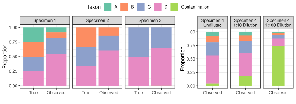
where is the unknown relative abundances of taxa and is a sampling intensity parameter (throughout, we let denote the closed -dimensional simplex). Unfortunately, microbial taxa are not detected equally well (Figure 1 (left); McLaren et al. (2019) and references therein). To account for this, we begin by considering the model
| (2) |
where represents the detection effects for taxa in a given experiment ( indicates element-wise multiplication). As an identifiability constraint, we set , and so interpret , as the degree of multiplicative over- or under-detection of taxon relative to taxon . We discuss identifiability in more detail in Section 3.
We now generalize model (2) to multiple samples and one or more experimental protocols. For a study involving samples of unique specimens (), we define the sample design matrix to link samples to specimens (). In most experiments, , but more complex designs are also possible (e.g., denotes that sample is a 1:1 mixture of specimens and ). Letting be a matrix such that the -th row of gives the true relative abundances of taxa in specimen , we have that the relative abundance vector for sample is . We allow differing detections across samples to be specified via the detection design matrix . For example, if samples are processed using one of different protocols, we might specify . Accordingly, we now consider a detection effect matrix , with as before. Therefore, one generalization of model (2) is
| (3) |
where , and where exponentiation is element-wise.
We now extend this model to reflect contributions of contaminant sources (Figure 1 (right)). We consider sources of contamination with relative abundance profiles given in the rows of . To link sources of contamination to samples, we let be a spurious read design matrix. Most commonly we expect , but we give an example of an analysis with more complex in Section 6.2. Then, along with contaminant read intensities , we propose to model
| (4) |
Here, is a diagonal matrix with diagonal elements equal to for design matrix and parameter . As discussed in more detail in Section 6.2, allows the intensity of contamination to vary across sources, but typically . Additionally, while we could incorporate a detection design matrix for contaminant reads (replacing (4) with for ), for most practical applications it is sufficient to identify up to detection effects. Therefore, combining models (3) and (4), we propose the following mean model for next-generation sequencing data :
| (5) |
3 Model identifiability
Our highly flexible mean model (5) encompasses a wide variety of experimental designs and targets of estimation. As a result, without additional knowledge, the parameters in the mean model (5) will generally be unidentifiable. We provide a general condition for identifiability in SI Lemma 1, and prove identifiability the following specific cases:
-
(a)
Estimating relative detectability under different sampling protocols using specimens of unknown composition (see SI Section 9.2 for identifiability; Section 6.1 for analysis)
-
(b)
Estimating contamination using dilution series (see SI Section 9.3 for identifiability; Section 6.2 for analysis)
-
(c)
Estimating contamination, detectability and composition when some samples have known composition (see SI Section 9.4 for identifiability; Section 7 for analysis)
In addition to knowledge of , and , constraints on the entries of and/or can result in the identifiability of model parameters. For example, in (c), some rows of are known. As mentioned previously, an identifiability constraint on (e.g., ) is always necessary.
4 Estimation and optimization
We propose to estimate parameters as M-estimators. We use likelihoods to define estimating equations but do not require or assume that the distribution of lies in any particular parametric class. We show consistency and weak convergence of our estimators of under mild conditions in SI Section 10. We use to denote the true value of . Our unweighted objective is given by a Poisson log-likelihood:
| (6) |
We use to indicate the profile log-likelihood , considering the elements of as sample-specific nuisance parameters. Consistency of for does not require to follow a Poisson distribution, however, the proposed estimator will be inefficient if the relationship between and is not linear (McCullagh, 1983). Therefore, to obtain a more efficient estimator, we also consider maximizing a reweighted Poisson log-likelihood, with weights chosen on the basis of a flexibly estimated mean-variance relationship. We motivate our specific choice of weights via the Poisson score equations (see SI Section 9). For weighting vector such that , we define the weighted Poisson log-likelihood as
| (7) |
We define by analogy with above. We select via a centered isotonic regression (Oron and Flournoy, 2017) of squared residuals on fitted means obtained from the unweighted objective. Full details are given in SI Section 10, but briefly, we set , where is the monotone regression fitted value for .
The estimators defined by optima of the weighted or unweighted Poisson likelihoods given above are consistent for the true value of and converge weakly to well-defined limiting distributions at rate, though the form of this distribution in general depends on the true value of . We leverage an approach from Van der Vaart (2000) to prove consistency, and we combine a bracketing argument with a directional delta method theorem of Dümbgen (1993) to show weak convergence. Proofs are given in SI Section 11.
Computing maximum (weighted) likelihood estimates of is a constrained optimization problem, as the relative abundance parameters in our model are simplex-valued, and the estimate may lie on the boundary of the simplex. Therefore, we minimize or in two steps. In the first step, we employ the barrier method, converting our constrained optimization problem into a sequence of unconstrained optimizations, permitting solutions progressively closer to the boundary. That is, for barrier penalty parameter , we update as
| (8) | ||||
| (9) |
and set where is a prespecified incrementing factor, iterating until for large . In practice we find that , , and yield good performance. We enforce the sum-to-one constraints (9) by reparametrizing and as and , with and for , which are well-defined because of the logarithmic penalty terms in (8).
In the second step of our optimization procedure, we apply a constrained Newton algorithm within an augmented Lagrangian algorithm to allow elements of and to equal zero. Iteratively in each row of , we approximately solve
| (10) |
where we write as a function of only to reflect that we fix all other parameters at values obtained in previous optimization steps. We choose update directions for via an augmented Lagrangian algorithm of Bazaraa (2006) applied to
| (11) |
where is a quadratic approximation to at and and are chosen using the algorithm of Bazaraa (2006). The augmented Lagrangian algorithm iteratively updates and until solutions to satisfy for a small prespecified value of (we use by default). Within each iteration of the augmented Lagrangian algorithm, we minimize via fast non-negative least squares to preserve nonnegativity of . Through the augmented Lagrangian algorithm, we obtain a value of that minimizes (at final values of and ) subject to nonnegativity constraints. Our update direction for is then given by . We conduct a backtracking line search in direction to find an update that decreases .
5 Inference for and
We now address construction of confidence intervals and hypothesis tests. We focus on parameters and , which we believe to be the most common targets for inference. To derive both marginal confidence intervals and more complex hypothesis tests, we consider a general setting in which we observe some estimate of population quantity , where is the empirical distribution corresponding to a sample , is its population analogue, and is a Hadamard directionally differentiable map into the parameter space or into . To derive marginal confidence intervals for and , we let with . For hypothesis tests involving multiple parameters, we specify as with population analogue under . In each case, we estimate the asymptotic distribution of for an appropriately chosen .
As our model includes parameters that may lie on the boundary of the parameter space, the limiting distributions of our estimators and test statistics in general do not have a simple distributional form (Geyer, 1994), and the multinomial bootstrap will fail to produce asymptotically valid inference (Andrews, 2000). To address this, we employ a Bayesian subsampled bootstrap (Ishwaran et al., 2009), which consistently estimates the asymptotic distribution of our estimators when the true parameter is on the boundary. Let be a weighted empirical distribution with weights for . Then the bootstrap estimator converges weakly to the limiting distribution of if we choose such that and (Ishwaran et al., 2009). We explore finite-sample behavior of the proposed bootstrap estimators with in Section 7, finding good Type 1 error control.
To derive marginal confidence intervals for elements of , we let and . Then has the same limiting distribution as . Therefore, for the -th bootstrap quantile of the -th element of and the -th element of the maximum (weighted) likelihood estimate , an asymptotically marginal confidence interval for is given by .
As it may be of interest to test hypotheses about multiple parameters while leaving other parameters unrestricted (e.g., with unrestricted elements of ), we also develop a procedure to test hypotheses of the form for a set of parameter indices against alternatives with unrestricted. Letting indicate the parameter space under and indicate the full parameter space, we conduct tests using test statistic . As noted above, is in general not asymptotically if (unknown) elements of or lie at the boundary, and so we instead approximate the null distribution of by bootstrap resampling from an empirical distribution projected onto an approximate null; this is closely related to the approach suggested by Hinkley (1988). Let denote times the expectation of under the full model; denote the analogous quantity under ; and define and otherwise set . In practice, we do not know or , so we replace with , where and are, up to proportionality constant , fitted means for under the full and null models. After constructing , we rescale its rows so row sums of and are equal. We then approximate the null distribution of via bootstrap draws from where is the Bayesian subsampled bootstrap distribution on . We reject at level if the observed likelihood ratio test statistic is larger than the quantile of the bootstrap estimate of its null distribution, or equivalently, if for the quantile of .
6 Data Examples
6.1 Comparing detection effects across experiments
We now demonstrate the utility of our model in comparing different experimental protocols for high-throughput sequencing of microbial communities. We consider data generated in the Phase 2 experiment of Costea et al. (2017) (see also McLaren et al. (2019)), wherein ten human fecal specimens (labeled , A and B) were mixed with a synthetic community of 10 taxa and prepared for shotgun metagenomic sequencing according to three different sample preparations (labeled H, Q, and W; samples A and B were only analyzed with preparation Q). The synthetic community was also sequenced alone. Raw sequencing data was processed into taxon abundance data using MetaPhlAn2 (Truong et al., 2015) by McLaren et al. (2019). In addition to sequencing data, taxon abundances in the synthetic community were also measured using flow cytometry. We treat both sequencing and flow cytometry measurements as outcomes . We are interested in comparing the detection of taxa in the synthetic community across protocols H, Q and W relative to flow cytometry. We are specifically interested in testing the null hypothesis that all sequencing protocols share the same detection effects. To accomplish this, we estimate the matrix (we set to ensure identifiability; see SI Section 9.2 for proof of identifiability). Each row of corresponds to a sequencing protocol, and each column corresponds to a taxon. For details regarding the specification of and other model parameters, see SI Section 13.1. Under our model, , , and give the degree of over- or under-detection of taxon relative to taxon 10 under protocols H, Q, and W, respectively. We compare this model to a submodel in which for and all . Under this null hypothesis, taxon detections relative to flow cytometry do not differ across protocols.
To compare predictive performance of these models, we perform 10-fold cross-validation on each model (see SI Section 13.2 for details). We use a bootstrapped likelihood ratio test to formally test our full model against the null submodel. We use the Bayesian subsampled bootstrap with to illustrate its applicability, however, a multinomial bootstrap would also be appropriate as all parameters are in the interior of the parameter space in this case. In addition, we report point estimates and bootstrapped marginal 95% confidence intervals for detection effects estimated for each protocol under the full model. We also compare our results to MetaPhlAn2’s “plug-in” estimate of each sample’s composition.
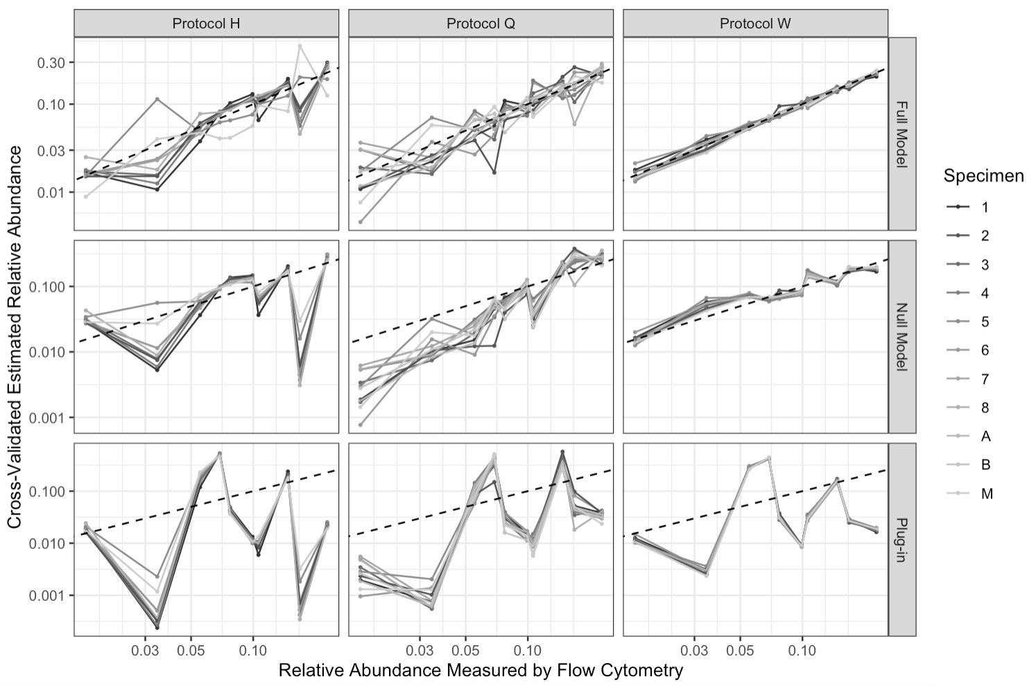
Figure 2 summarizes 10-fold cross-validated estimated relative abundances from the full model, null model and plug-in estimates. We observe substantially better model fit for the full model (top row) than for the null model (middle row). At each flow cytometric relative abundance, cross-validated estimates from the full model are generally centered around the line (dotted line), whereas estimates from the null model exhibit substantial bias for some taxa. A bootstrapped likelihood ratio test of the null model (i.e., ) against the full model reflects this, and we reject the null with . Both the full and null models outperform the plug-in estimates of sample composition (bottom row), which produces substantially biased estimates of relative abundance relative to a flow cytometry standard. We report point estimates and marginal 95% confidence intervals for in SI Section 13.3.
Using the full model, we estimate relative abundances with substantially greater precision under protocol W (top right) than under either other protocol (top left and center). This appears to be primarily due to lower variability in measurements taken via protocol W (bottom row). Our finding of greater precision of protocol W contrasts with Costea et al. (2017), who recommend protocol Q as a “potential benchmark for new methods” on the basis of median absolute error of centered-log-ratio-transformed plug-in estimates of relative abundance against flow cytometry measurements (as well as on the basis of cross-laboratory measurement reproducibility, which we do not examine here). The recommendations of Costea et al. (2017) are driven by performance of plug-in estimators subject to considerable bias, whereas we are able to model and remove a large degree of bias and can hence focus on residual variation after bias correction. We also note that Costea et al. (2017) did not use MetaPhlAn2 to construct abundance estimates, which may partly account our different conclusions.
6.2 Estimating contamination via dilution series
We next illustrate how to use our model to estimate and remove contamination in samples. We consider 16S rRNA sequencing data from Karstens et al. (2019), who generated 9 samples via three-fold dilutions of a synthetic community containing 8 distinct strains of bacteria which each account for 12.5% of the DNA in the community. Despite only 8 strains being present in the synthetic community, 248 total strains were identified based on sequencing (see SI Section 14.1 for data processing details). We refer to the 8 strains in the synthetic community as “target” taxa and other strains as “off-target.” Note that Karstens et al. (2019) identified one strain as a likely mutant of synthetic community member S. enterica, and we refer to this strain as S. [unclassified].
To evaluate the performance of our model, we perform three-fold cross-validation and estimate relative abundance in the hold-out fold. We consider , where the first row contains the known composition of the training fold and the second row is unknown and the target of inference (see SI Section 14.2 for full model specification). We evenly balance dilutions across folds, and using our proposed reweighted estimator to fit a model that accounts for the serial dilutions. We set and let , where is the number of three-fold dilutions sample has undergone. This model reflects the assumption that the ratio of expected contaminant reads to expected non-contaminant reads is proportional to . To avoid improperly sharing information about contamination amounts across folds, we include terms in a fixed, unknown parameter in . In particular, we let design matrix by which we premultiply consist of a single column vector with -th entry 1 if sample is in the held-out fold and 0 otherwise. This preserves information about relative dilution within the held-out fold without treating samples in the training and held-out folds as part of the same dilution series. That is, the source of contamination for the held-out fold is modeled to be the same as in the training fold, but intensity of contamination for held-out sample having undergone three-fold dilutions is given by as compared to for a sample in the training set. We model a single differential detection effect for each of the 8 taxa in the synthetic community, setting for the reference taxon L. fermentum for identifiability. Because is not identifiable for off-target taxa, we also fix for (see SI Section 9.3 for identifiability results).
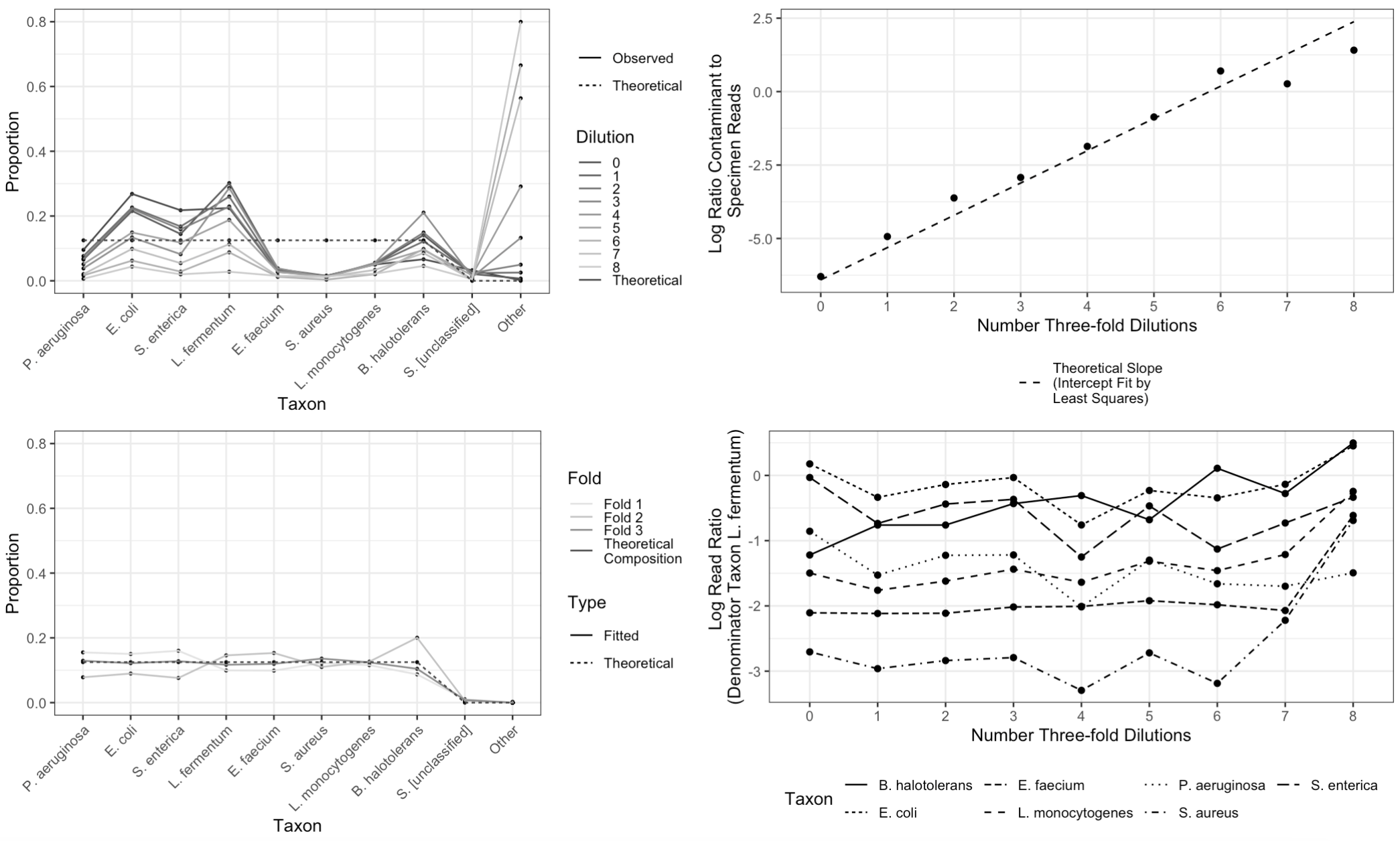
Figure 3 shows data from Karstens et al. (2019) along with summaries of our analysis. Our estimate for the relative abundance of taxa in samples in the held-out fold improves on the performance of plug-in estimators (Figure 3, left panels) by taking into account two forms of structure in the Karstens et al. (2019) data. First, in each successive three-fold dilution, we observe approximately three times more contamination relative to the number of non-contaminant reads (Figure 3, top right). In addition, our model accounts for the degree of under- (or over-) detection of target taxa relative to L. fermentum. We observe that taxon detection is reasonably constant across dilutions (Figure 3, bottom right). However, we do observe greater variability in taxon detections at higher dilutions, most likely because we observe comparatively few reads ( while ).
In terms of root mean squared error (RMSE) , our cross-validated estimates (, , and ) substantially outperform the “plug-in” estimates given by sample read proportions in any of these dilutions (median ; range – ). This is not an artifact of incorporating information from 3 samples in each cross-validation fold, as pooling reads across all samples yields an estimator with RMSE .
Fitting a model to this relatively small dataset and evaluating its performance using cross validation prohibits the reasonable construction of confidence intervals. Therefore, to evaluate the performance of our proposed approach to generating confidence intervals, we also fit a model which treats all samples as originating from a single specimen of unknown composition. is not identifiable in this setting, so we set it equal to zero and do not estimate it. We set and as before (the need for is alleviated). Strikingly, under this model, marginal 95% confidence intervals for elements of included zero for 238 out of 240 off-target taxa (empirical coverage of when true ). No interval estimates for target taxa included zero. This suggests that applying our proposed approach to data from a dilution series experiment can aid in evaluating whether taxa detected by next-generation sequencing are actually present in a given specimen.
7 Simulations
7.1 Sample size and predictive performance
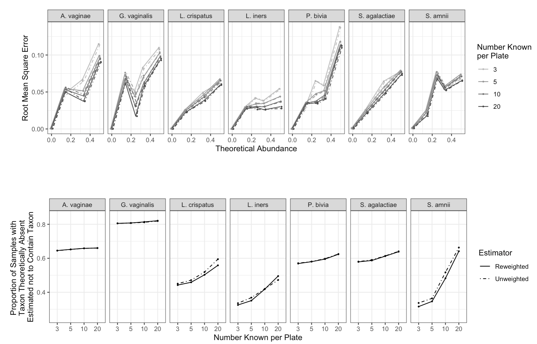
To evaluate the predictive performance of our model on microbiome datasets of varying size, we use data from 65 unique specimens consisting of synthetic communities of 1, 2, 3, 4, or 7 species combined in equal abundances. Brooks et al. (2015) performed 16S amplicon sequencing on 80 samples of these 65 specimens across two plates of 40 samples each. Very few reads in this dataset were ascribed to taxa outside the 7 present by design, so we limit analysis to these taxa. To explore how prediction error varies with number of samples of known composition, we fit models treating randomly selected subsets of samples per plate as known. In each model, we included one source of unknown contamination for each plate and estimate a detection vector . For each , we drew 100 independent sets of samples to be treated as known, requiring that each set satisfy an identifiability condition in (see SI Section 9.4). On each set, we fit both the unweighted and reweighted models, treating samples as having known composition and samples as arising from unique specimens of unknown composition.
We observe similar RMSE for the reweighted and unweighted estimators. For equal to 3, 5, 10, and 20, we observe RMSE 0.041, 0.037, 0.035, and 0.032 (to 2 decimal places) for both estimators. By comparison, the RMSE for the plugin estimator is 0.173. Notably, RMSE decreases but does not approach zero as larger number of samples are treated as known, which reflects that we estimated each relative abundance profile on the basis of a single sample.
With respect to correctly estimating when , we again see very similar performance of the reweighted and unweighted Poisson estimators. Out of 100 sets, unweighted estimation yields for , and of pairs for which ( equal to 3, 5, 10, and 20). The corresponding figures for the reweighted estimator are , and . The plug-in estimator sets of these relative abundances equal to zero. While we observe the proportion of theoretical zero relative abundances estimated to be zero increases in number of samples treated as known regardless of estimator, in general we do not expect this proportion to approach 1 as number of known samples increases. We also note that our model is not designed to produce prediction intervals, and confidence intervals for a parameter estimated from a single observation are unlikely to have reasonable coverage. Finally, we acknowledge that despite the excellent performance of our model on the data of Brooks et al. (2015), our model does not fully capture sample cross-contamination known as index-hopping (Hornung et al., 2019), which likely affects this data.
7.2 Type 1 error rate and power
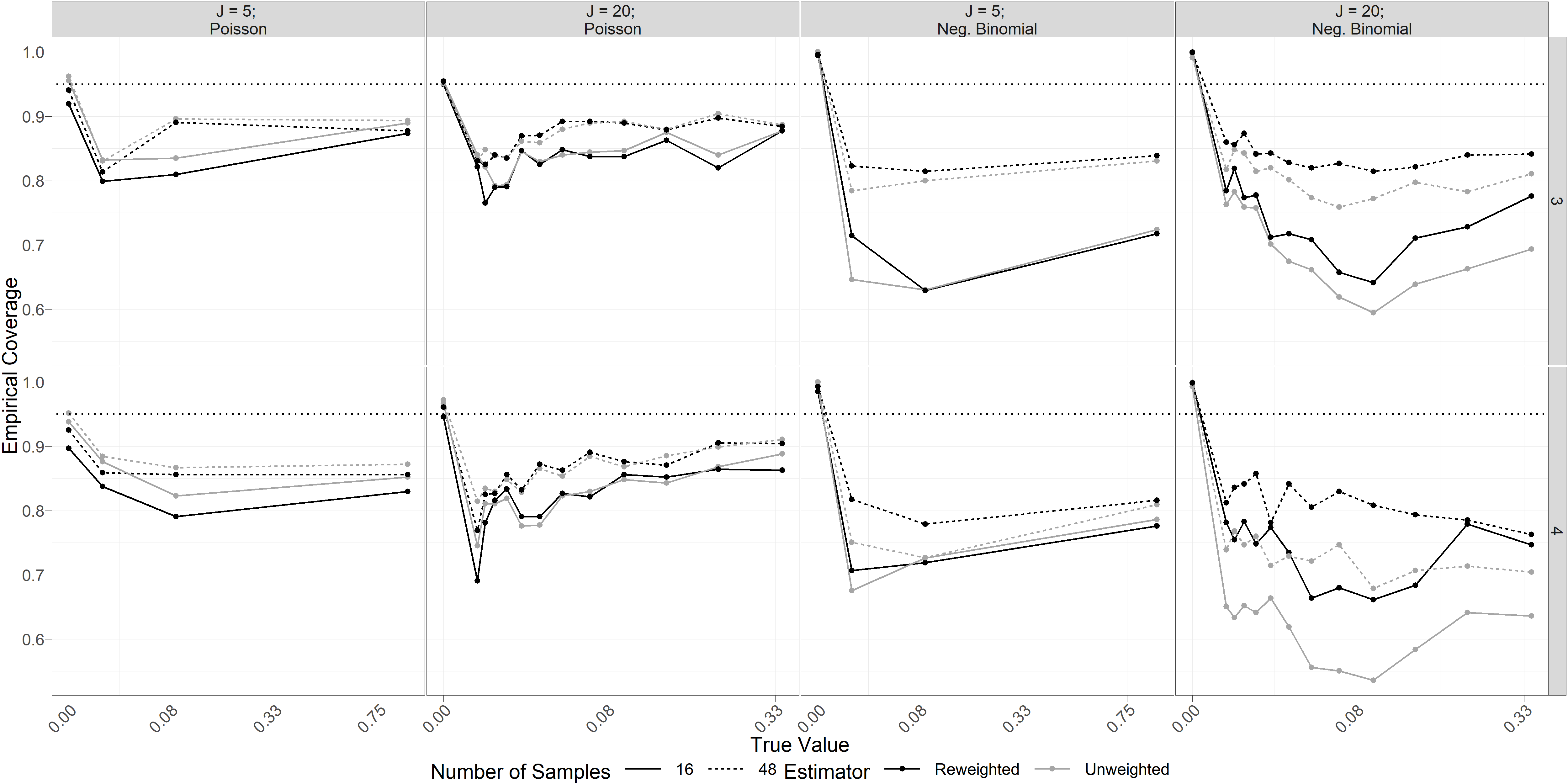
To investigate the Type 1 error rate and power of tests based on reweighted and unweighted estimators, we simulate data arising from a set of hypothetical dilution series. In each simulated dataset, we observe reads from dilution series of four specimens: two specimens of known composition and two specimens of unknown composition (specimens A and B). Each dilution series consists of four samples: an undiluted sample from a specimen as well as a 9-, 81-, and 729-fold dilution of the specimen. We vary the number of taxa , as well as the magnitude of elements of , the number of samples, and the distribution of . The identifiability results of SI Section 9.3 apply here.
We consider three different values of : , , and where when and when . We base the magnitude of entries of using the observed magnitude of entries of in our analysis of Costea et al. (2017) data. We vary the number of samples between either a single dilution series from each specimen or three dilution series from each specimen (for a total of nine samples per specimen). We draw from either a Poisson() distribution or a Negative Binomial distribution with mean parameter and size parameter . was chosen to approximate the Karstens et al. (2019) data via a linear regression of fitted mean-centered squared residuals. In all settings we simulate from a log-normal distribution with parameters and . These values were chosen based on observed trends in reads from target taxa in the data of Karstens et al. (2019) data. In all settings, the first specimen has true relative abundance proportional to , that is, taxon is 16 times more abundant than taxon 1. The second specimen has true relative abundance proportional to . When , the first two taxa are absent from specimen A, and when , first eight taxa are absent from specimen A. Relative abundances in the remaining taxa form an increasing power series such that the first taxon present in nonzero abundance has relative abundance that is -th of the relative abundance of taxon . The relative abundance profile of specimen B is given by the relative abundance vector for specimen A in reverse order. We also simulate the degree of contamination as scaling with dilution. When comparing samples with the same read depth, on average a 9-fold diluted sample will contain 9 times more contaminant reads than an undiluted sample (see Section 5.2 and Figure 3, top right). We simulate contamination from a source containing equal relative abundance of all taxa. We set such that where is the degree of dilutions of sample , and , as we observe in Karstens et al. (2019) data.
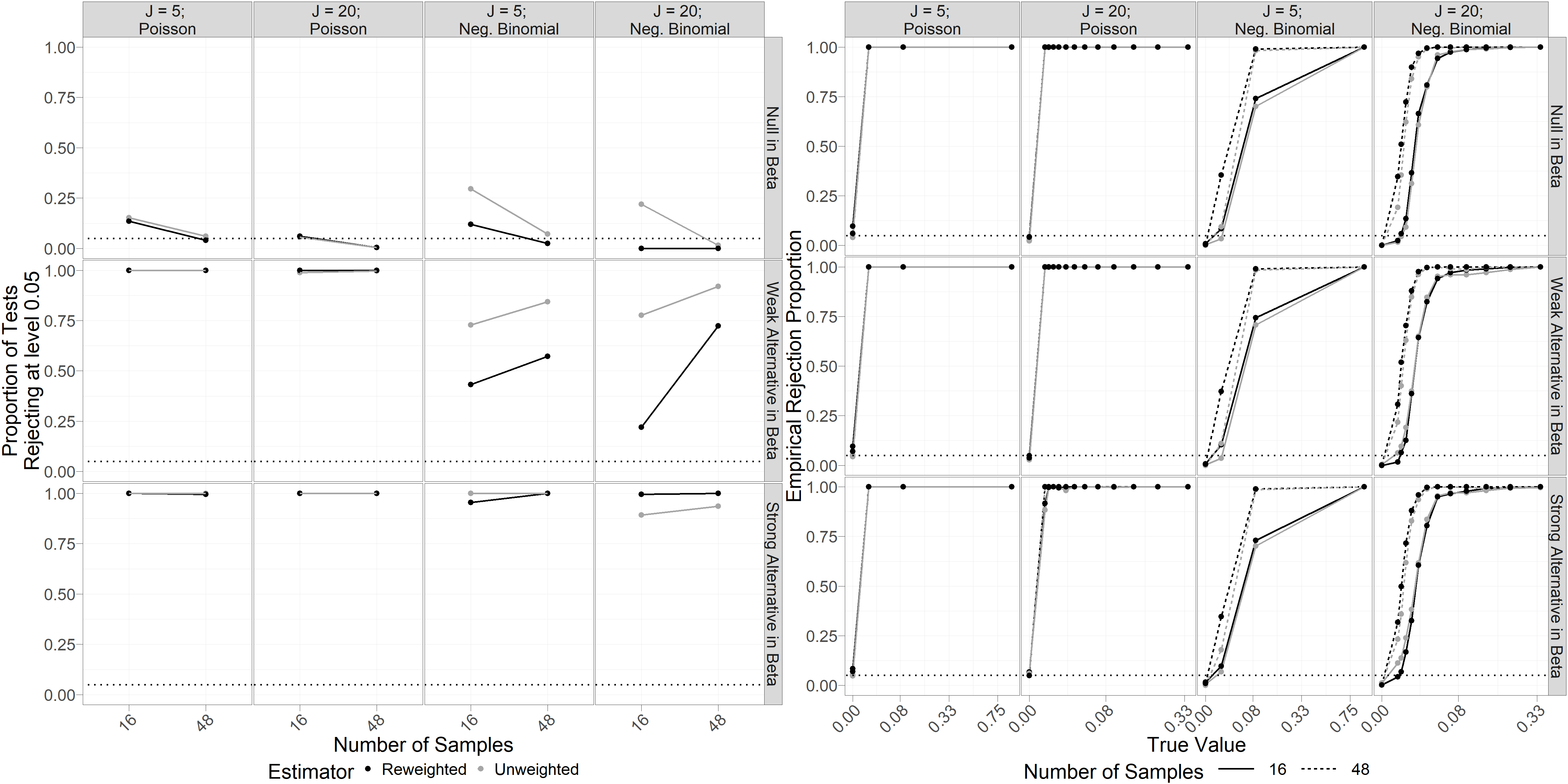
Figure 4 summarizes our results from 250 simulations under each condition. Empirical performance of bootstrapped likelihood ratio tests of against at level 0.05 (lefthand pane of Figure 4) reveals good performance, even for small sample sizes. Unsurprisingly, we observe improved Type 1 error control and power at larger sample sizes. Tests based on the reweighted estimator generally improved Type 1 error compared to the unweighted estimator, with the greatest improvements observed for data simulated from a negative binomial distribution (mean Type 1 error across simulations was 0.15 for the unweighted estimator and 0.04 for the reweighted estimator). Surprisingly, Type 1 error control appears to improve when the number of taxa is larger (mean Type 1 error was 0.11 for and 0.05 for ). This may in part be a result of simulating as conditionally independent given , covariates, and other parameters. Power to reject the null hypothesis is very high when the data generating process is Poisson, as well as for strong alternatives () when the data follows a negative binomial distribution.
Empirical Type 1 error control for bootstrapped marginal tests of against at the 0.05 level (lefthand pane of Figure 4) is generally no larger than nominal, with median empirical Type 1 error across all conditions. We observe above-nominal Type 1 error in limited cases, primarily when sample size is small and data is Poisson-distributed (the largest observed Type 1 error rate, of 0.10, occurs for tests based on reweighted estimators at sample size and number of taxa when data is Poisson-distributed). Power to reject the null is close to 1 for all non-zero values of when data is conditionally Poisson-distributed (median empirical power across conditions 1; minimum 0.88). When data is simulated as negative binomial, unsurprisingly, power appears to increase in magnitude of for tests based on unweighted and reweighted estimators, with somewhat higher power in tests using reweighted estimators. Magnitude of (rows of Figure 4) does not appear to affect Type 1 error or power of our tests of . We also note that empirical coverage of marginal bootstrapped confidence intervals for is generally lower than nominal in our simulations (SI Figure 2). This aligns with general performance of bootstrap percentile confidence intervals at small sample sizes, and we expect that generating confidence intervals from inverted bootstrapped likelihood ratio tests would yield better coverage in this case (unfortunately this is not feasible for computational reasons).
8 Discussion
In this paper, we introduce a statistical method to model measurement error due to contamination and differential detection of taxa in microbiome experiments. Our method builds on previous work in several ways. By directly modeling the output of microbiome experiments, we do not rely on data transformations that discard information regarding measurement precision, such as ratio- or proportion-based transformations. This affords our method the key advantage of estimating relative abundances lying on the boundary of the simplex, which is typically precluded by transformation-based approaches. Accordingly, we implement inference tools appropriate to the non-standard parameter space that we consider. The advantage of estimating relative abundances on the boundary of the simplex is not purely theoretical, and we show that our interval estimates do indeed include boundary values, and demonstrate above-nominal empirical coverage in an analysis of data from Karstens et al. (2019). Furthermore, our reweighting estimator allows for flexible mean-variance relationships without the need to specify a parametric model. Our approach to parameter estimation does not assume that observations are counts, and therefore our method can be applied to a wide array of microbiome data types, including proportions, coverages and cell concentrations as well as counts. Finally, our method can accommodate complex experimental designs, including analysis of mixtures of samples, technical replicates, dilution series, detection effects that vary by experimental protocol or specimen type, and contamination impacting multiple samples. Contamination is commonly addressed via “pre-processing” data, thereby conditioning on the decontamination step. In contrast, by simultaneously estimating contamination along with all other model parameters, our approach captures holistic uncertainty in estimation.
Another advantage of our methodology is that we do not require the true composition of any specimens to be known. For example, our test of equal detection effects across protocols in Costea et al. (2017) can be performed without knowledge of specimen composition. Accordingly, our approach provides a framework for comparing experimental protocols in the absence of synthetic communities, which can be challenging to construct.
In addition, we expect that our method may have substantial utility applied to dilution series experiments, as illustrated in our analysis of data from Karstens et al. (2019). Dilution series are relatively low-cost and scalable (especially in comparison to synthetic communities) and may be especially advantageous when the impact of sample contamination on relative abundance estimates is of particular concern. With this said, we strongly recommend against testing the composite null against the point alternative , as these hypotheses are statistically indistinguishable on the basis of any finite sample of reads. However, we are able to determine the degree to which our observations are consistent with the absence of any given taxon, and therefore we can meaningfully test against a general alternative.
The focus of our paper was on and as targets of inference. Future research could investigate extensions to our model that connect relative abundances to covariates of interest, allowing the comparison of average relative abundances across groups defined by covariates, for example. Our proposed bootstrap procedures may also aid the propagation of uncertainty to group-level comparisons of relative abundances in downstream analyses. In addition, while we focus applications of our model on microbiome data, our model could be applied to a broad variety of data structures obtained from high-throughput sequencing, such as single-cell RNAseq. We leave these applications to future work.
9 SI: Identifiability
As discussed in the main text, our model is flexible enough to encompass a wide variety of experimental designs and targets of estimation, but as a result, the parameters in model (5) are unidentifiable without additional constraints. In this section, we demonstrate identifiability for the three use cases of our model that we considered as illustrative examples. For reference, we provide here the definition of identifiability:
Definition 0.1.
A mean function is said to be identifiable if
9.1 Preliminaries
We first consider situations where contamination is not modelled (e.g., Section 6.1), and as such, . In this case, the following Lemma provides a sufficient condition under which mean model (5) may be reparametrized as a log-linear model. Since a log-linear model is identifiable if and only if its design matrix has full column rank, this result provides a basis on which to establish identifiability for a large subclass of models.
Unless otherwise noted, without loss of generality we take throughout.
Lemma 1.
Let denote a mean function for an matrix such that the -th element of is given by , for the -th element of , the -th column of (for a matrix with rows in the -simplex), the -th column of the matrix , and and the -th rows of and , respectively. If each row of lies in the interior of and each row of contains a single nonzero entry , equal to 1, then there exists a matrix for and an isomorphism such that for all , for the -th row of .
Proof.
It suffices to show the result holds for an arbitrary element of , say, . Let be the unique index such that . We have
We let , which is trivially an isomorphism. is then given by
| (12) |
where is the Kronecker product, has -th element equal to 1 and all others 0, has -th element equal to 1 and all others 0, and has -th element equal to 1 and all others zero (when , contains only zeroes). Matrix multiplication then gives . ∎
Theorem 1.
Under the conditions of Lemma 1, then mean function is identifiable if and only if has full column rank.
Proof.
We proceed by contradiction for both directions. () Suppose satisfies the criteria given in Lemma 1 and is not identifiable. For , this implies that for some s.t. . This in turn implies that since has full column rank. Since is an isomorphism, we have , and therefore, a contradiction. Hence must be identifiable if is full rank. () Now suppose is not full rank. Then for some , . Letting be an arbitrary vector in , we have and hence . Since is an isomorphism, we must have , and hence the mean function is not identifiable. ∎
The above results apply when all rows of are unknown. However, when some rows of are known, we may establish identifiability of the unknown parameters under the conditions of Lemma 1 by considering the rank of the matrix obtained from by excluding columns corresponding to any element of for such that is known.
9.2 Identifiability: Comparing detection effects across experiments
In Section 6.1, we analyzed data consisting of measurements taken via three sequencing protocols on human fecal samples containing a spiked-in artificial community in addition to measurements taken via flow cytometry on the spiked-in community (Costea et al., 2017). We constrained our analysis to taxa in the spiked-in community, which by design are present in every sample. In this setting, we may apply Theorem 1.
We first show identifiability of the mean function defined for models fit without cross-validation, and then address models fit via cross-validation. We assume familiarity with the experimental setup and notation introduced in Section 6.1. We adopt the identifiability constraint .
9.2.1 Model without Cross-Validation
In the model fit without cross-validation, all samples originate from a single source. The mean for sample is given by
| (13) |
where parametrizes sample intensity, is a matrix of detection effects (here, ), is the unknown relative abundance profile for the sample from which our observations were taken, and
for and indicators for sample being processed according to protocol or , respectively. Thus, from (12), the form of is
Hence the submatrix of consisting of rows corresponding to taxa through in sample is given by where is a column -vector of ones and is the identity matrix with -th column removed. Since there are 4 unique rows of , the leftmost columns of are spanned by the rows of
Since this is a full-rank matrix, the matrix consisting of the leftmost columns of must have full column rank. It now remains to show that the rightmost columns of are linearly independent of the leftmost and compose a matrix with full column rank. The latter is immediate from inspection, and the former follows from the fact that the leftmost columns of contain rows of zeroes (corresponding to observations on taxon ), whereas the rightmost columns contain no zero rows and hence must be linearly independent of the remainder of the columns. Theorem 1 therefore applies and we have established identifiability of this model.
9.2.2 Cross-Validated Model
The cross-validated version of the above model differs only in the addition of an extra row of corresponding to the composition of the specimen from which samples in the held-out fold are taken. This yields a model we can express as a log-linear model with nearly the same design matrix as above. Namely, we have such that the the submatrix consisting of rows corresponding to sample is given by
where is an indicator that sample is in the held-in fold, and analogously for . There are now 8 rather than 4 unique rows in columns of :
This is again a full-rank matrix, and thus the columns of corresponding to and are linearly independent. Consequently, Theorem 1 applies and thus the mean model is identifiable.
9.3 Identifiability: Estimating contamination via dilution series
In Section 6.2, we analyze a serial dilution of a specimen of known composition (Karstens et al., 2019). In this application, we estimated a contamination profile, and therefore the conditions of Theorem 1 do not apply. In the following sections we thus establish identifiability of the model directly. We consider the two cases discussed in the manuscript (fitting with and without cross-validation) separately.
9.3.1 Two sources; estimated via cross-validation
We first consider identifiability of parameters in the model fit using cross-validation in Section 14.2. For sample in the training set, the mean model is
where is the (known) true relative abundance vector of the synthetic community, gives (unknown) intensity of contamination in an undiluted sample from the reference, is the (unknown) contaminant relative abundance vector, and represents the (known) number of three-fold dilutions sample has undergone. For sample in the held-out/test set, the mean model is
| (14) |
where is the unknown relative abundance vector, and is the (unknown) intensity of contamination in an undiluted test set sample.
The inclusion of a contaminant profile requires additional identifiability constraints. For example, as noted in the main text, we fix for all such that . In addition, we require that there is a taxon, call it , that is present in the synthetic community (), present in the test set sample (), and absent from the contaminant profile (). Finally, we require that the “reference taxon” for interpreting is present in the synthetic community. We may choose any reference taxon other than . As usual, we take .
We proceed via contrapositive, beginning with the training fold. Suppose
| (15) |
Equation (15) for taxon gives , and thus
| (16) |
Now, consider distinct samples in the training fold such that . Subtracting (16) for sample from (16) for sample , with the latter rescaled by , and cancelling terms, yields
| (17) |
and thus such that . Combining this with , noting that , and recalling that all other elements of are constrained to equal zero, we have that that . Plugging this into equation (16) gives and summing over and simplifying gives both and . Since all other parameters in (15) are now identified, we have for in the training fold. Thus all parameters are identified for the training fold.
Turning now to the held-out test fold, we again proceed by contrapositive. , , and are identifiable from the training fold and thus we consider
| (18) |
As above, we divide by the mean for taxon on both sides to obtain
| (19) |
We now subtract (19) for sample from (19) for sample (; both and in the test fold) then simplifies to give
| (20) |
Recalling that (18) for taxon gives , and thus
| (21) |
Additionally, by the same argument that yielded equation (17),
| (22) |
and therefore . Since both must sum to 1, Combining this with (20) gives and (21) gives for in the test fold. Hence the parameters in the test fold are also identified.
9.3.2 Single source; no cross-validation
To investigate the empirical coverage of confidence intervals for the elements of , we also considered a model where all samples are derived from a single source. No detection efficiencies are estimated in this model, which has mean
| (23) |
We demonstrate identifiability assuming again that for known , and . Taking the same approach as above, we have that
| (24) |
Dividing this expression by the mean for taxon , and subtracting the resulting expression for sample by the resulting expression for sample , we have
| (25) |
Summing over and rearranging, we obtain . Also, since , we have , and so . We substitute this into (24) to obtain
| (26) |
Summing over gives and therefore and therefore also and . Equation (25) then gives and finally follows from (24).
9.4 Identifiability: Estimating detectability, composition and contamination via samples of known composition
In Section 7.1, we used data from Brooks et al. (2015) to study the prediction error of our model as a function of the number of samples of known composition, randomly selecting sets of samples to treat as known. In this model, we have unknown detection efficiencies, an unknown contamination profile, an unknown contamination intensity, unknown sample detection effects, and unknown composition for some samples. We do, however, have known composition for some samples. Specifically, for sample of known composition, we have
| (27) |
for , , and unknown and known. For sample of unknown composition, we have
with and unknown. Critically, , and are shared across the samples of known and unknown composition.
Consider a graph with nodes, each representing a taxon, and connect all nodes if there exists a sample of known composition such that both and . For identifiability in , we require that this graph is connected. For simultaneous identifiability of detection efficiencies and contamination profiles, we also require that all taxa are absent from at least two samples of known composition, and we assume that contamination profiles lie in the interior of the -simplex.
9.4.1 Identifiability in samples of known composition
We begin by demonstrating identifiability of the parameters present in the samples of known composition. Proceeding via contrapositive, if the mean model is not identifiable in we must have that
with .
We first demonstrate identifiability in . Define . Then, and for two samples and . Then, for , rearranging gives , so if , . Since we assumed that all taxa are absent from at least two samples of known composition, the desired samples and must exist, and therefore , which implies that (both sides must sum to 1). Therefore, is identifiable in this model.
Before showing identifiability in the remaining parameters , we first prove the following lemma guaranteeing that identifiability of these model parameters does not depend on which we choose in defining our identifiability constraint on .
Lemma 1.
For any , given and , the model specified in (27) is identifiable in under the constraint if and only if it is identifiable in these parameters under constraint .
Proof.
Let denote an element of , and similarly for and . Note that defines a bijection from into . Since it is sufficient to show identifiability for an arbitrary sample , we proceed by constructing a bijection such that . For arbitrary ,
That is, defines a bijection from into such that . As such, if we have that
under (for arbitrary ), then the same must hold for arbitrary . This is because otherwise we could find such that
which would be a contradiction. Therefore, identifiability under implies identifiability under . Finally, it is immediate that lack of identifiability under implies lack of identifiability under . If there exists with , and , then is a pair in with the same property. ∎
We now show identifiability in . For such that for at least one , consider the identifiability constraint for some such that (which is WLOG by the above lemma). Then if , we have and thus , from which we have
since . Now choose another sample with and at least one other nonzero entry of (by assumption such an exists). If in taxon we have
| (28) |
this immediately implies since and (as both equal under our identifiability constraint). Now let denote another taxon such that . If we have
| (29) |
this implies . For arbitrary , this argument allows us to show identifiability in given identifiability in conditional on the existance of an such that and . Since we assume connectedness of the graph whose nodes are taxa with an edge between two nodes if and for some known sample , we are guaranteed to be able to find a path starting at taxon and visiting each other taxon at least once such that for any adjacent in our path, there exists a known sample with and . Hence by induction with base case , we have if for arbitrary we have . Finally, given identifiability of and , identifiability of for any sample of known composition is trivial. Hence the mean model is identifiable in all parameters that appear in the mean model for samples treated as known.
9.4.2 Identifiability in samples of unknown composition
We now turn our attention to parameters appearing only in samples treated as of unknown composition. For such a sample, a lack of identifiability now would entail
for . This immediately gives us
from which we have
Summing over , we obtain
which implies , which in turn implies that for a sample treated as of unknown composition. Hence the model is identifiable in these parameters as well.
Note that while we have given sufficient conditions for a model with a single source of contamination, the same argument applies to multiple (including plate-specific) sources of contamination, since does not vary across plate.
10 SI: Additional details for reweighted estimator
In Section 4, we introduced a weighted Poisson log-likelihood with weight for the likelihood contribution of given by
where is the fitted mean for given parameters estimated under a Poisson likelihood and read depth . arising from a model fit to via a Poisson likelihood (without reweighting) and is a fitted value from a monotone regression of squared residuals on fitted means (with and ). In other words, is an estimate of .
To motivate why this reweighting is reasonable, we consider the case in which is in the interior of the parameter space . In this setting we can express the Poisson MLE as a solution to the following score equations:
Equivalently, we can write
letting . Hence, we can view this system of equations as a weighted sum of zero expectation terms with weights given by –– that is, one over a model-based estimate of . In this setting, if the Poisson mean-variance relationship holds and the score equations have a unique solution, we expect the estimator given by this solution to be asymptotically efficient (McCullagh, 1983), whereas when a different mean-variance relationship holds, in general we expect to lose efficiency. In contrast, when the Poisson mean-variance relationship does not hold, we expect to be able to improve efficiency by reweighting the score equations with a more flexible estimator of . To accomplish this, we use a consistent estimator of , the Poisson MLE , to estimate and . Specifically, we estimate under the assumption that is an increasing function via a centered isotonic regression of on . Weighting the log-likelihood contribution of , , by a factor of then yields reweighted score equations
in which each is, up to a factor of , weighted by the inverse of a flexible estimate of . In practice, however, the weighting above may be unstable when and are small. Hence, we weight instead by to preserve behavior of weights when the estimated mean and variance are both large (where reweighting is typically most important) and stabilizes them when these quantities are small.
11 SI: Supporting theory for proposed model and estimators
Throughout this section, we will use the following notation:
-
•
: a measured outcome of interest in sample across taxa . We also use without subscript where this does not lead to ambiguity
-
•
here denotes covariates described in the main text
-
•
: the support of
-
•
: the support of
-
•
: the support of
-
•
: a weighting function from into . For simplicity of notation, we frequently suppress dependence on and and write to indicate
-
•
: an empirical weighting function estimated from a sample of size
-
•
: unknown parameters ; we denote the true value with
-
•
: a parametrization of the mean model given in equation (5) in main text; ; when unambiguous, we suppress dependence on and write ; we also use to denote
-
•
: profile log-likelihood under weighting function , evaluated at on a sample of size
-
•
: expected profile log-likelihood under weighting function , evaluated at
-
•
: the profile log-likelihood under weighting function as a function from into ; , and similarly we can express in terms of and the empirical measure :
-
•
: the set of all uniformly bounded real functions on
11.1 Assumptions
-
(A)
We draw pairs where has closed, bounded support and has closed, bounded support .
-
(B)
Letting denote , for a set of known functions from to we have that where , with differentiable in for all and for each fixed , a bounded function on .
-
(C)
For almost all , for some .
Note: while the form of the mean model given above differs somewhat from the presentation in the main text, it in fact implies the form in the main text if we introduce random variable and let . However, since this construction in terms of is not necessary for the results that follow, we omit it.
11.2 Form of profile log-likelihood
We first derive the form of a log-likelihood in which nuisance parameters , have been profiled out. We characterize population analogue of this log-likelihood. The form of this profile log-likelihood is as follows:
| (30) | ||||
| (31) |
where we suppress dependence on for simplicity in the second row. We derive the profile likelihood in the second row via differentiation with respect to ; the optimum is unique by convexity of in when . We use to denote and similarly for .
We now allow weights to be given as a (bounded positive) function of and and examine the population analogue of of the weighted profile log-likelihood .
| (32) | ||||
| (33) | ||||
| (34) | ||||
| (35) | ||||
| (36) |
We note that the term in line 5 above depends on but not ; accordingly, we represent it with constant on line 7.
11.3 Optimizer of profile likelihood
We now show that, under a suitable identifiability condition, a weak condition on , and a condition on weighting function , that if the mean model given in assumption B holds at , then the unique optimizer of population criterion is .
The additional conditions we need are as follows:
-
(D)
For all , we have that, for any , holds for all with .
-
(E)
Weighting function , where is the support of , is continuous and bounded.
We will use the following simple lemma:
Lemma 2.
For every , the function defined by is uniquely maximized at (defining and letting for every ).
Proof.
First consider the case . Since in this case and is finite for all , the optimum cannot occur at . Over , , so is strictly convex over and hence takes a unique optimum. Setting gives us that the optimum occurs at .
When , , so is optimized at since when . ∎
Theorem 1.
Suppose that conditions (A) - (D) are met. Then for any weighting function satisfying (E), the criterion defined above is uniquely optimized at .
Proof.
From above we have the form of the population criterion :
| (37) |
For each fixed pair , denote by the function . Then
| (38) |
is maximized when by Lemma 1. ∎
Before proceeding, we show that . By definition, we have
| (39) | ||||
| (40) | ||||
| (41) | ||||
| (42) |
The term in line (41) is equal to , which as the integral of a bounded function over a bounded domain is finite. By assumption (C), we must have almost surely, so the term in line (42) is almost surely bounded by boundedness of , , and . Inside the sum in this line, we have terms of the form , which is a bounded function on any bounded set in . Hence line (42) is an integral of a bounded function over a bounded domain and so is also finite, so .
Similarly,
| (43) | ||||
| (44) | ||||
| (45) |
Hence , which guarantees that the difference in the following argument is not of the form .
Now, for any with , we have
The first inequality is a result of maximizing (not necessarily uniquely) ; i.e., . Strict inequality holds in the last line because the integrand in is strictly negative, since for on , and the term is a.s. strictly positive by assumption (C) and positivity of . Hence for all in , so is the unique maximizer of the population criterion .
11.4 Consistency of M-estimators
We apply theorem 5.14 of van der Vaart (1998) to show consistency of maximizers of for . We also show consistency of estimators , where is a sequence of random continuous positive bounded weighting functions converging uniformly in probability to .
We first require the following assumption on ,, and :
-
(F)
and every is continuous, positive, and bounded.
-
(G)
There exist and such that holds for all where is a closed -neighborhood of in . Moreover, is Lipschitz continuous in on for each .
Note: while assumption (G) can likely be loosened, we note that in practice it is not particularly restrictive. In particular, we emphasize that it in no way precludes from lying at the boundary of the parameter space; rather, it guarantees that nonzero means are bounded away from zero, which allows us to select neighborhoods of in which is bounded.
Theorem 2.
Suppose conditions (A) through (G) are satisfied. Then for , for all and for all .
Proof
We first compactify our parameter space to obtain by allowing elements of unconstrained Euclidean parameters to take values in the extended reals.
A necessary condition for theorem 5.14 is that we have for and a sufficiently small ball . By Lemma 1, , which is bounded above since is bounded. Hence by assumption (A), . We also require which is trivially satisfied since maximizes .
Then letting compact set , we can directly apply theorem 5.14 to obtain for any .
To apply theorem 5.14 to , we only need in addition to the above that .
For any fixed , we have
| (46) | ||||
| (47) |
However, the term if we let since, letting ,
| (48) | ||||
| (49) |
since . Hence , so for any .
11.5 Convergence in distribution of M-estimators
Theorem 3.
If assumptions A - E are met, converges in distribution to a tight limiting distribution in .
Proof.
Without loss of generality, we consider for given in assumption G (since by theorem 2, with probability approaching , as increases without bound).
We begin by considering criterion without weighting.
Fix . We then have, for any ,
| (50) |
By Lipschitz continuity of in over , is a Lipschitz continuous function at all such that all elements of are nonzero since is Lipschitz continuous for and bounded . When one or more elements of are zero, they must be identically over all ; otherwise by continuity of in , we are able to select such that is positive but arbitrarily close to zero, contradicting assumption G.
Since if , we must have with probability 1 (on account of being a nonnegative random variable), except possibly on a set with measure , we have
| (51) |
Accordingly, is Lipschitz continuous in for all . Hence , as a weighted sum of Lipschitz continuous functions (with bounded weights), must also be Lipschitz continuous for all as well.
We now use a bracketing argument to show that is a Donsker class, which we will use together with a result due to Dümbgen (1993) to show that converges to a well-defined limiting distribution in .
By Lipschitz continuity of in on , we have
| (52) |
for some .
Hence we can consider
| (53) | ||||
| (54) |
where
where Lipschitz continuity of guarantees the existence of the limit as .
Hence by Lipschitz continuity of in and continuity of in and , is continuous in , and , which in turn implies that is continuous on and hence is bounded on by compactness of . Since by assumption is bounded, this implies that is integrable, which is sufficient for the bracketing entropy of to be at most of order (see Van der Vaart (2000) example 19.7). Hence by theorem 19.5 of Van der Vaart (2000), is Donsker.
Accordingly, we have weakly converging to a tight Gaussian process in as . By proposition 1 of Dümbgen (1993), this, taken with Hadamard directional differentiability of the map defined by , gives us
| (55) |
for well-defined limiting distribution on .
∎
Theorem 4.
converges in distribution to the same limit as if assumptions A - G are met.
Proof.
| (56) | ||||
| (57) | ||||
| (58) | ||||
| (59) |
since
| (60) | ||||
| (61) | ||||
| (62) |
Note that by theorem 1. ∎
12 SI: Optimization details
12.1 Reparametrization of barrier subproblem
Letting indicate the unknown parameters in our model after reparametrizing and as and , we now have the following unconstrained minimization problem:
| (63) | ||||
| (64) |
12.2 Barrier algorithm
Barrier Algorithm 1. Initiate with value of penalty parameter set to starting value and values of parameters equal to . Set iteration . 2. Using current value of and starting at parameter estimate , solve barrier subproblem r given in main text via Fisher scoring. Denote the solution of this subproblem and set for a prespecified . 3. If for prespecified , return . Otherwise set iteration and return to step 2.
12.3 Constrained Newton within Augmented Lagrangian Algorithm
We calculate update steps from given in Section 4 of the main text as follows:
Constrained Newton within Augmented Lagrangian Algorithm 1. Initiate with initial values and of penalty coefficients and 2. Calculate proposed update via nonnegative least squares on using current values of and 3. If for some prespecified tolerance , set update direction and proceed to step (3). Otherwise update and via algorithm given in Bazaraa (2006) (p. 496) and return to step (1). 4. Perform a line search in direction to determine updated parameter value that decreases objective for some .
12.4 Quadratic approximation to .
In Section 4 of the main text, we specify in terms of a quadratic approximation to objective . In practice we construct as a slightly modified Taylor expansion of around the current value of . We use the gradient of with respect to in the first order term, and in the second order term, and in place of the Hessian, we use ( times) the Fisher information matrix in regularized (for numerical stability) by addition of magnitude of the gradient times an identity matrix.
13 SI: Analysis of Costea et al. (2017) data
13.1 Details of model specification
Costea et al. (2017) published two flow cytometric readings for every species in the synthetic community with the exception of V. cholerae, for which only one reading was published. In all taxa save V. cholerae, we take the mean reading as our observation, and we include the resulting vector of readings augmented by the single reading for V. cholerae as a row in . We anticipate that our use of mean readings represents a fairly small loss of information, as flow cytometric readings did not vary substantially within taxon. However, in a similar setting where multiple sets of flow cytometric readings across all taxa were available, we could include each set as a row of to capture variability in these measurements.
To estimate detection effects relative to flow cytometry measurements, we specify . For , where is an indicator for sample being processed according to protocol Q, and similarly for .
13.2 Cross-validation design
We construct folds for our 10-fold cross-validation on Costea et al. (2017) data so that, with the exception of samples A and B, which we grouped together in a single fold, each fold included all observations for a given specimen. For each fold, we fit a model in which all observations in all other folds, along with flow cytometry readings, were treated as arising from a common specimen (as in fact they do, save for flow cytometry readings, which were taken on specimens mixed to create the mock spike-in). We model each sample in the held-out fold as arising from a distinct specimen of unknown composition to allow our model to estimate a different relative abundance profile for distinct samples processed according to different protocols.
13.3 Model summaries
| Taxon | Protocol H | Protocol Q | Protocol W |
|---|---|---|---|
| B. hansenii | -1.61 (-2.00 – -1.16) | -1.55 (-1.75 – -1.31) | -0.08 (-0.16 – 0.00) |
| C. difficile | -0.18 (-0.30 – 0.01) | -0.57 (-0.79 – -0.41) | 1.23 (1.18 – 1.28) |
| C. perfringens | 3.38 (3.27 – 3.57) | 2.48 (2.31 – 2.62) | 4.05 (4.03 – 4.07) |
| C. saccharolyticum | -0.19 (-0.23 – -0.16) | -0.01 (-0.12 – 0.1) | -0.10 (-0.13 – -0.06) |
| F. nucleatum | 2.37 (2.28 – 2.44) | 0.14 (-0.16 – 0.42) | 2.11 (2.05 – 2.16) |
| L. plantarum | -2.62 (-2.96 – -2.12) | 0.72 (0.60 – 0.93) | 0.60 (0.56 – 0.63) |
| P. melaninogenica | 4.17 (4.12 – 4.2) | 3.88 (3.82 – 4.04) | 4.25 (4.23 – 4.27) |
| S. enterica | 2.49 (2.45 – 2.51) | 2.74 (2.64 – 2.79) | 2.48 (2.46 – 2.51) |
| V. cholerae | 1.54 (1.50 – 1.56) | 0.90 (0.78 – 0.99) | 1.48 (1.44 – 1.50) |
Table 1 provides point estimates and marginal confidence intervals for the detection effects for each of protocols H, Q, and W estimated via the full model described above. This model was fit with reference taxon Y. pseudotuberculosis (i.e., under the constraint that the column of corresponding to this taxon consists of entries). Hence we interpret estimates in this table in terms of degree of over- or under-detection relative to Y. pseudotuberculosis – for example, we estimate that, repeated measurement under protocol H of samples consisting of 1:1 mixtures of B. hansenii and Y. pseudotuberculosis, the mean MetaPhlAn2 estimate of the relative abundance of B. hansenii will be as large as the mean estimate of the relative abundance of Y. pseudotuberculosis.
14 SI: Analysis of Karstens et al. (2019) data
14.1 Preprocessing
We process raw read data reported by Karstens et al. (2019) using the DADA2 R package (version 1.20.0) (Callahan et al., 2016). We infer amplicon sequence variants using the dada function with option ‘pooled = TRUE’ and assign taxonomy with the assignSpecies function using a SILVA v138 training dataset downloaded from https://benjjneb.github.io/dada2/training.html (Quast et al., 2012).
14.2 Model Specification
We conduct a three-fold cross-validation of a model containing both contamination and detection effects. For each held-out fold , if we let , , and indicate element-wise multiplication then we specify the model for this fold with
The relative abundance matrix consists of two rows, the first of which is treated as fixed and known and contains the theoretical composition of the mock community used by Karstens et al. (2019). The second row is to be estimated from observations on samples in the held-out fold. consists of a single row, the first 247 elements of which we treat as unknown. We fix as an identifiability constraint – identifiability problems arise here because all samples sequenced arise from the same specimen, we lack identifiability over, for any choice of fixed and , the set . Briefly, we do not consider the assumption unrealistic; while in general distinguishing between contaminant and non-contaminant taxa is challenging, it is fairly frequently the case that choosing a single taxon unlikely to be a contaminant is not difficult. Moreover, we anticipate that in most applied settings, more than one specimen will be sequenced and this identifiability problem will hence not arise.
consists of a single row, the first elements of which (corresponding to contaminant taxa) are treated as fixed and known parameters equal to 0, as we cannot estimate detection efficiencies in contaminant taxa. The following 7 elements of are treated as fixed and unknown (to be estimated from data), and is set equal to 0 as an identifiability constraint. is specified as a single unknown parameter in
The full model fit without detection efficiencies is specified by treating as fixed and known with all elements equal to 0. We treat all samples as arising from the same specimen, so , , and consists of a single row treated as an unknown relative abundance. Specifications of , , , and are specified as above.
14.3 Additional summaries
| Taxon | Estimate |
|---|---|
| P. aeruginosa | -1.29 |
| E. coli | -0.20 |
| S. enterica | -0.48 |
| E. faecium | -2.09 |
| S. aureus | -3.05 |
| L. monocytogenes | -1.60 |
| B. halotolerans | -0.74 |
For each taxon for which is identifiable (i.e., taxa in the mock community), our model produces a point estimate , as shown in table 2. (The reference taxon, L. fermentum, for which we enforce identifiability constraint , is excluded.) On the basis of this model, we estimate that in an equal mixture of E. coli and our reference taxon, L. fermentum sequenced by the method used by Karstens et al. (2019), we expect on average to observe E. coli reads for each L. fermentum read. In an equal mixture of S. aureus and L. fermentum similarly sequenced, we expect on average to observe reads for each L. fermentum read.
15 SI: Simulation results based on Brooks et al. (2015) data
15.1 Figures
Figure 5 summarizes performance of cross-validated models fit to Brooks et al. (2015) data. Briefly, we observe very similar performance comparing unweighted and weighted estimators both in terms of root mean square error (RMSE) and proportion of elements of estimated to be 0. RMSE is generally smaller for models fit on larger training sets, but it does not approach zero as training set size increases. We also observe a strong relationship between RMSE and theoretical true relative abundance, which likely reflects a strong mean-variance relationship in the data.
We also observe generally a greater proportion of elements of estimated to be zero with increasing training set size, although the degree to which this occurs depends on taxon. Weighting does not appear to have a large impact on this measure of predictive performance.
16 SI: Simulations with Artificial Data
Figure 6 summarizes empirical coverage of marginal bootstrap 95% confidence intervals for elements of obtained from simulations described in the main text. As discussed in the main text, coverage is high for but falls when . Unsurprisingly, we observe higher coverage at larger sample sizes. Coverage of intervals based on reweighted estimators appears to be slightly lower than for unweighted estimators when data is Poisson-distributed (lefthand columns), but intervals using reweighted estimators substantially outperform unweighted intervals when data is negative binomial distributed, particularly when number of taxa is larger.
References
- Andrews (2000) Andrews, D.W. (2000). Inconsistency of the bootstrap when a parameter is on the boundary of the parameter space. Econometrica, 399–405.
- Bazaraa (2006) Bazaraa, M.S. (2006). Nonlinear programming: theory and algorithms.
- Brooks et al. (2015) Brooks, J.P. et al (2015). The truth about metagenomics: quantifying and counteracting bias in 16s rrna studies. BMC Microbiology 15(1), 1–14.
- Callahan et al. (2016) Callahan, B.J. et al (2016). DADA2: high-resolution sample inference from illumina amplicon data. Nature Methods 13(7), 581.
- Costea et al. (2017) Costea, P.I. et al (2017). Towards standards for human fecal sample processing in metagenomic studies. Nature Biotechnology 35(11), 1069.
- Dai et al. (2019) Dai, Z. et al (2019). Batch effects correction for microbiome data with dirichlet-multinomial regression. Bioinformatics 35(5), 807–814.
- Davis et al. (2018) Davis, N.M. et al (2018). Simple statistical identification and removal of contaminant sequences in marker-gene and metagenomics data. Microbiome 6(1), 1–14.
- Dümbgen (1993) Dümbgen, L. (1993). On nondifferentiable functions and the bootstrap. Probability Theory and Related Fields 95(1), 125–140.
- Fernandes et al. (2014) Fernandes, A.D. et al (2014). Unifying the analysis of high-throughput sequencing datasets: characterizing rna-seq, 16s rrna gene sequencing and selective growth experiments by compositional data analysis. Microbiome 2, 1–13.
- Gagnon-Bartsch and Speed (2012) Gagnon-Bartsch, J.A. and Speed, T.P. (2012). Using control genes to correct for unwanted variation in microarray data. Biostatistics 13(3), 539–552.
- Geyer (1994) Geyer, C.J. (1994). On the asymptotics of constrained m-estimation. The Annals of Statistics, 1993–2010.
- Gibbons et al. (2018) Gibbons, S.M., Duvallet, C. and Alm, E.J. (2018). Correcting for batch effects in case-control microbiome studies. PLoS Computational Biology 14(4), e1006102.
- Hinkley (1988) Hinkley, D.V. (1988). Bootstrap methods. Journal of the Royal Statistical Society: Series B (Methodological) 50(3), 321–337.
- Hornung et al. (2019) Hornung, B.V., Zwittink, R.D. and Kuijper, E.J. (2019). Issues and current standards of controls in microbiome research. FEMS Microbiology Ecology 95(5), fiz045.
- Ishwaran et al. (2009) Ishwaran, H., James, L.F. and Zarepour, M. (2009). An alternative to the m out of n bootstrap. Journal of Statistical Planning and Inference 139(3), 788–801.
- Johnson et al. (2007) Johnson, W.E., Li, C. and Rabinovic, A. (2007). Adjusting batch effects in microarray expression data using empirical bayes methods. Biostatistics 8(1), 118–127.
- Karstens et al. (2019) Karstens, L. et al (2019). Controlling for contaminants in low-biomass 16s rrna gene sequencing experiments. MSystems 4(4), e00290–19.
- Knights et al. (2011) Knights, D. et al (2011). Bayesian community-wide culture-independent microbial source tracking. Nature Methods 8(9), 761–763.
- Leek and Storey (2007) Leek, J.T. and Storey, J.D. (2007). Capturing heterogeneity in gene expression studies by surrogate variable analysis. PLoS genetics 3(9), e161.
- Li et al. (2021) Li, Z. et al (2021). Ifaa: robust association identification and inference for absolute abundance in microbiome analyses. Journal of the American Statistical Association 116(536), 1595–1608.
- Love et al. (2014) Love, M.I., Huber, W. and Anders, S. (2014). Moderated estimation of fold change and dispersion for rna-seq data with deseq2. Genome Biology 15, 1–21.
- Mallick et al. (2021) Mallick, H. et al (2021). Multivariable association discovery in population-scale meta-omics studies. PLoS Computational Biology 17(11), e1009442.
- Mandal et al. (2015) Mandal, S. et al (2015). Analysis of composition of microbiomes: a novel method for studying microbial composition. Microbial Ecology in Health and Disease 26(1), 27663.
- Martin et al. (2019) Martin, B.D., Witten, D. and Willis, A.D. (2019). Modeling microbial abundances and dysbiosis with beta-binomial regression . arXiv.
- McCullagh (1983) McCullagh, P. (1983). Quasi-likelihood functions. The Annals of Statistics 11(1), 59–67.
- McLaren et al. (2019) McLaren, M.R., Willis, A.D. and Callahan, B.J. (2019). Consistent and correctable bias in metagenomic sequencing experiments. eLife 8.
- Oron and Flournoy (2017) Oron, A.P. and Flournoy, N. (2017). Centered isotonic regression: point and interval estimation for dose–response studies. Statistics in Biopharmaceutical Research 9(3), 258–267.
- Quast et al. (2012) Quast, C. et al (2012). The silva ribosomal rna gene database project: improved data processing and web-based tools. Nucleic Acids Research 41(D1), D590–D596.
- Shenhav et al. (2019) Shenhav, L. et al (2019). Feast: fast expectation-maximization for microbial source tracking. Nature Methods 16(7), 627–632.
- Silverman et al. (2021) Silverman, J.D. et al (2021). Measuring and mitigating pcr bias in microbiota datasets. PLoS Computational Biology 17(7), e1009113.
- Sims et al. (2008) Sims, A.H. et al (2008). The removal of multiplicative, systematic bias allows integration of breast cancer gene expression datasets–improving meta-analysis and prediction of prognosis. BMC Medical Genomics 1(1), 1–14.
- Truong et al. (2015) Truong, D.T. et al (2015). Metaphlan2 for enhanced metagenomic taxonomic profiling. Nature Methods 12(10), 902–903.
- Van der Vaart (2000) Van der Vaart, A.W. (2000). Asymptotic statistics, Volume 3. Cambridge university press.
- Zhao and Satten (2021) Zhao, N. and Satten, G.A. (2021). A log-linear model for inference on bias in microbiome studies. In Statistical Analysis of Microbiome Data, pp. 221–246. Springer.