Modeling for Dynamic Ordinal Regression Relationships: An Application to Estimating Maturity of Rockfish in California
Abstract
We develop a Bayesian nonparametric framework for modeling ordinal regression relationships which evolve in discrete time. The motivating application involves a key problem in fisheries research on estimating dynamically evolving relationships between age, length and maturity, the latter recorded on an ordinal scale. The methodology builds from nonparametric mixture modeling for the joint stochastic mechanism of covariates and latent continuous responses. This approach yields highly flexible inference for ordinal regression functions while at the same time avoiding the computational challenges of parametric models. A novel dependent Dirichlet process prior for time-dependent mixing distributions extends the model to the dynamic setting. The methodology is used for a detailed study of relationships between maturity, age, and length for Chilipepper rockfish, using data collected over 15 years along the coast of California.
KEY WORDS: Chilipepper rockfish; dependent Dirichlet process; dynamic density estimation; growth curves; Markov chain Monte Carlo; ordinal regression
1 Introduction
Consider ordinal responses collected along with covariates over discrete time. Furthermore, assume multiple observations are recorded at each point in time. This article develops Bayesian nonparametric modeling and inference for a discrete time series of ordinal regression relationships. Our aim is to provide flexible inference for the series of regression functions, estimating the unique relationships present at each time, while introducing dependence by assuming each distribution is correlated with its predecessors.
Environmental characteristics consisting of ordered categorical and continuous measurements may be monitored and recorded at different points in time, requiring a model for the temporal relationships between the environmental variables. The relationships present at a particular point in time are of interest, as well as any trends or changes which occur over time. Empirical distributions in environmental settings may exhibit non-standard features including heavy tails, skewness, and multimodality. To capture these features, one must move beyond standard parametric models in order to obtain more flexible inference and prediction.
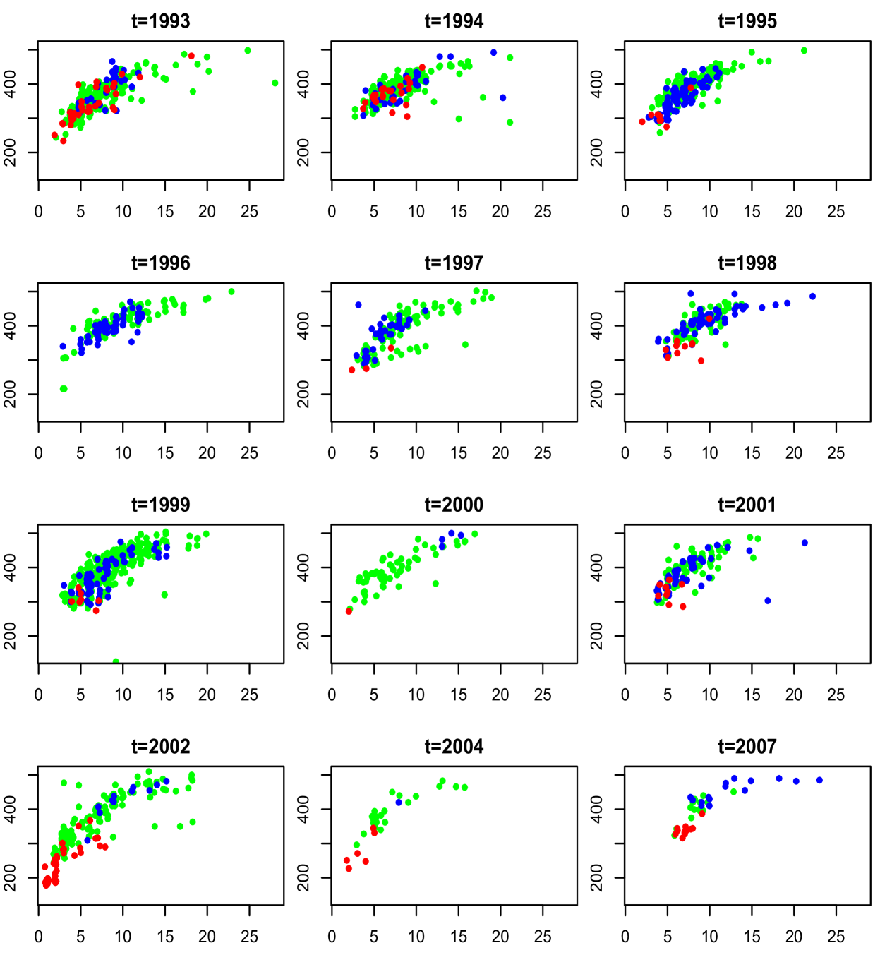
The motivating application for this work lies in modeling fish maturity as a function of age and length. This is a key problem in fisheries science, one reason being that estimates of age at maturity play an important role in population estimates of sustainable harvest rates (Clark, 1991; Hannah et al., 2009). The specific data set comes from the National Marine Fisheries Service and consists of year of sampling, age recorded in years, length in millimeters, and maturity for female Chilipepper rockfish, with measurements collected over 15 years along the coast of California. Maturity is recorded on an ordinal scale, with values taken to be from through , where indicates immature and and represent pre- and post-spawning mature, respectively. More details on the data are provided in Section 3. Exploratory analysis suggests both symmetric, unimodal as well as less standard shapes for the marginal distributions of length and age; histograms for three years are shown in Figure 1. Bivariate data plots of age and length suggest similar shapes across years, with some differences in location and scale, and clear differences in sample size, as can be seen from Figure 2. To make the plot more readable, random noise has been added to age, which is recorded on a discretized scale. Maturity level is also indicated; red color represents immature, green pre-spawning mature, and blue post-spawning mature. Again, there are similarities including the concentration of immature fish near the lower left quadrants, but also differences such as the lack of immature fish in years through as compared to the early and later years.

In addition to studying maturity as a function of age and length, inference for the age and length distributions is also important. This requires a joint model which treats age and length as random in addition to maturity. We are not aware of any existing modeling strategy for this problem which can handle multivariate mixed data collected over time. Compromising this important aspect of the problem, and assuming the regression of maturity on body characteristics is the sole inferential objective, a possible approach would be to use an ordered probit regression model. Empirical (data-based) estimates for the trend in maturity as a function of length or age indicate shapes which may not be captured well by a parametric model. For instance, the probability a fish is immature (level 1) is generally decreasing with length, however, in some of the years, the probability a fish is post-spawning mature (level 3) is increasing up to a certain length value and then decreasing. This is not a trend that can be captured by parametric models for ordinal regression (Boes and Winkelmann, 2006, discuss some of these properties). One could include higher order and/or interaction terms, though it is not obvious which terms to include, and how to capture the different trends across years.
In practice, virtually all methods for studying maturity as a function of age and/or length use logistic regression or some variant, often collapsing maturity into two levels (immature and mature) and treating each covariate separately in the analysis (e.g., Hannah et al., 2009; Bobko and Berkeley, 2004). Bobko and Berkeley (2004) applied logistic regression with length as a covariate, and to obtain an estimate of age at maturity (the age at which of fish are mature), they used their estimate for length at maturity and solved for the corresponding age given by the von Bertalanffy growth curve, which relates age to length using a particular parametric function. Others assume that maturity is independent of length after conditioning on age, leading to inaccurate estimates of the proportion mature at a particular age or length (Morgan and Hoenig, 1997).
We develop a nonparametric Bayesian model to study time-evolving relationships between maturation, length, and age. These three variables constitute a random vector, and although maturity is recorded on an ordinal scale, it is natural to conceptualize an underlying continuous maturation variable. Distinguishing features of our approach include the joint modeling for the stochastic mechanism of maturation and length and age, and the ability to obtain flexible time-dependent inference for multiple ordinal maturation categories. While estimating maturity as a function of length and age is of primary interest, the joint modeling framework provides inference for a variety of functionals involving the three body characteristics.
Our goal is to construct a modeling framework for dynamic ordinal regression which avoids strict parametric assumptions and possesses features that make it well-suited to the fish maturity application, as well as to similar evolutionary biology problems on studying natural selection characteristics (such as survival or maturation) in terms of phenotypic traits. To this end, we build on previous work on ordinal regression not involving time (DeYoreo and Kottas, 2014a), where the ordinal responses arise from latent continuous variables, and the joint latent response-covariate distribution is modeled using a Dirichlet process (DP) mixture of multivariate normals (Müller et al., 1996). In the context of the rockfish data, we model maturity, length, and age jointly, using a DP mixture. This modeling approach is further developed here to handle ordinal regressions which are indexed in discrete time, through use of a new dependent Dirichlet process (DDP) prior (MacEachern, 1999, 2000), which estimates the regression relationship at each time point in a flexible way, while incorporating dependence across time.
We review the model for ordinal regression without the time component in Section 2.1. Section 2.2 introduces the DDP, and in Section 2.3, we develop a new method for incorporating dependence in the DP weights to handle distributions indexed in discrete time. The model is then developed further in Section 3 in the context of the motivating application, and applied to analyze the rockfish data discussed above. Section 4 concludes with a discussion. Technical details on properties of the DDP prior model, and on the posterior simulation method are included in the appendixes.
2 Modeling Framework
2.1 Bayesian Nonparametric Ordinal Regression
We first describe our approach to regression in the context of a single distribution, that is, without any aspect of time. Let denote the data, where each observation consists of an ordinal response along with a vector of covariates . The methodology is developed in DeYoreo and Kottas (2014a) for multivariate ordinal responses, however we work with a univariate response for notational simplicity and because this is the relevant setting for the application of interest. Our model assumes the ordinal responses arise as discretized versions of latent continuous responses, which is natural for many settings and particularly relevant for the fish maturity application, as maturation is a continuous variable recorded on a discrete scale. With categories, introduce latent continuous responses such that if and only if , for , and cut-offs .
We focus on settings in which the covariates may be treated as random, which is appropriate, indeed necessary, for many environmental applications. In the fish maturity example, the body characteristics are interrelated and arise in the form of a data vector, and we are interested in various relationships, including but not limited to the way in which maturity varies with age and length. This motivates our focus on building a flexible model for the joint density , for which we apply a DP mixture of multivariate normals: , with .
By the constructive definition of the DP (Sethuraman, 1994), a realization from a is almost surely of the form . The locations are independent realizations from the centering distribution , and the weights are determined through stick-breaking from beta distributed random variables. In particular, let , , independently of , and define , and for , . Therefore, the model for has an almost sure representation as a countable mixture of multivariate normals, and implies the following induced model for the regression function:
| (1) |
with covariate-dependent weights , covariate-dependent means , and variances . Here, is partitioned into and according to and , and are the components of the corresponding partition of covariance matrix .
This modeling strategy allows for non-linear, non-standard relationships to be captured, and overcomes many limitations of standard parametric models. In addition, the cut-offs may be fixed to arbitrary increasing values (which we recommend to be equally spaced and centered at zero) without sacrificing the ability of the model to approximate any distribution for mixed ordinal-continuous data. In particular, it can be shown that the induced prior model on the space of mixed ordinal-continuous distributions assigns positive probability to all Kullback-Leibler neighborhoods of any distribution in this space. This represents a key computational advantage over parametric models. We refer to DeYoreo and Kottas (2014a) for more details on model properties, a review of existing approaches to ordinal regression, and illustration of the benefits afforded by the nonparametric joint model over standard methods. This discussion refers to ordinal responses with three or more categories. For the case of binary regression, i.e., when , additional restrictions are needed on the covariance matrix to facilitate identifiability (DeYoreo and Kottas, 2014b).
2.2 Dependent Dirichlet Processes
In developing a model for a collection of distributions indexed in discrete time, we seek to build on previous knowledge, retaining the powerful and well-studied DP mixture model marginally at each time , with . We thus seek to extend the DP prior to model , a set of dependent distributions such that each follows a DP marginally. The dynamic DP extension can be developed by introducing temporal dependence in the weights and/or atoms of the constructive definition, .
The general formulation of the DDP introduced by MacEachern (1999, 2000) expresses the atoms , as independently and identically distributed (i.i.d.) sample paths from a stochastic process over , and the latent beta random variables which drive the weights, , , as i.i.d. realizations from a stochastic process with beta marginal distributions. The distributions could be indexed in time, space, or by covariates, and represents the corresponding index set, being in our case. The DDP model for distributions indexed in discrete time expresses as , for . The locations are i.i.d. for , from a time series model for the kernel parameters. The stick-breaking weights , , arise through a latent time series with beta marginal distributions, independently of .
The general DDP can be simplified by introducing dependence only in the weights, such that the atoms are not time dependent, or alternatively, the atoms can be time dependent while the weights remain independent of time. We refer to these as common atoms and common weights models, respectively. While the majority of DDP applications fall into the common weights category, we believe the most natural of the two simplifications for time series is to assume that the locations are constant over time, and introduce dependence in the weights. Although we will end up working with the more general version of the DDP with dependent atoms and weights, for the application and related settings, it seems plausible that there is a fixed set of factors that determine the region in which the joint density of body characteristics is supported, but dynamics are caused by changes in the relative importance of the factors. The construction of dependent weights requires dependent beta random variables, so that , , for , with each a realization from a time series model with beta() marginals. Equivalently, we can write , , for , with each a realization from a time series model with beta() marginals.
There have been many variations of the DDP model proposed in the literature. The common weights version was originally discussed by MacEachern (2000), in which a Gaussian process was used to generate dependent locations, with the autocorrelation function controlling the degree to which distributions which are “close” are similar, and how quickly this similarity decays. De Iorio et al. (2004) consider also a common weights model, in which the index of dependence is a covariate, a key application of DDP models. In the order-based DDP of Griffin and Steel (2006), covariates are used to sort the weights. Covariate dependence is incorporated in the weights in the kernel and probit stick-breaking models of Dunson and Park (2008) and Rodriguez and Dunson (2011), respectively, however these prior models do not retain the DP marginally. Gelfand et al. (2005) developed a DP mixture model for spatial data, using a spatial Gaussian process to induce dependence in DDP locations indexed by space. For data indexed in discrete time, Rodriguez and ter Horst (2008) apply a common weights model, with atoms arising from a dynamic linear model. Di Lucca et al. (2013) develop a model for a single time series of continuous or binary responses through a DDP in which the atoms are dependent on lagged terms. Xiao et al. (2015) construct a dynamic model for Poisson process intensities built from a DDP mixture with common weights and different types of autoregressive processes for the atoms. Taddy (2010) assumes the alternative simplification of the DDP with common atoms, and models the stick-breaking proportions using the positive correlated autoregressive beta process from McKenzie (1985). Nieto-Barajas et al. (2012) also use the common atoms simplification of the DDP, modeling a time series of random distributions by linking the beta random variables through latent binomially distributed random variables.
2.3 A Time-Dependent Nonparametric Prior
To generate a correlated series such that each marginally, we define a stochastic process
| (2) |
which is built from a standard normal random variable and an independent stochastic process with standard normal marginal distributions. This transformation leads to marginal distributions for any . To see this, take two independent standard normal random variables and , such that follows an exponential distribution with mean 1, and thus . To our knowledge, this is a novel construction for a common atoms DDP prior model. The practical utility of the transformation in (2) is that it facilitates building the temporal dependence through Gaussian time-series models, while maintaining the DP structure marginally.
Because we work with distributions indexed in discrete time, we assume to be a first-order autoregressive (AR) process, however alternatives such as higher order processes or Gaussian processes for spatially indexed data are possible. The requirement of standard normal marginal distributions on leads to a restriction on the variance of the AR(1) model, such that , . Thus , which implies stationarity for the stochastic process . Since is a transformation of a strongly stationary stochastic process, it is also strongly stationary. Note that the correlation in is driven by the autocorrelation present in , and this induces dependence in the weights , which leads to dependent distributions .
We now explore this dependence, discussing some of the correlations implied by this prior model. First, consider the correlation of the beta random variables used to define the dynamic stick-breaking weights. Let , which is equal to under the assumption of an AR(1) process for . The autocorrelation function associated with is
| (3) |
as described in Appendix A. Smaller values for lead to smaller correlations for any fixed at a particular lag, and controls the strength of correlation, with large producing large correlations which decay slowly. The parameters and in combination can lead to a wide range of correlations, however implies a lower bound near on the correlation for any lag . In the limit, as , , and as , tends towards as , and as . Assuming , gives and This tends upwards to quickly as .
Note that is a function of but not , which is to be expected since enters the expression for only through , and thus and have the same effect in the correlation. The same is true of the correlation in the DP weights, which is given below. We believe that is a natural restriction, since we are building a stochastic process for distributions correlated in time through a transformation of an AR process, which intuition suggests should be positively correlated. However, all that is strictly required to preserve the DP marginals is .
Assuming is generated by , from an underlying AR(1) process for with coefficient , we study the dependence induced in the resulting DDP weights at consecutive time points, . The covariance is given by
| (4) |
which can be divided by to yield ; note that and . Derivations are given in Appendix A. This expression is decreasing in index , and larger values of lead to larger correlations in the weights at any particular . Moreover, the decay in correlations with weight index is faster for small and small . As , for any value of , and as , is contained in , with values closer to for larger . Note that has the same expression as , but with replaced by ; it is thus decreasing with the lag , with the speed of decay controlled by .
Finally, assume is a random distribution on , such that , where the are defined through the dynamic stick-breaking weights , and the are i.i.d. from a distribution on . Consider two consecutive distributions , and a measurable subset . The correlation of consecutive distributions, , is discussed in Appendix A.
3 Estimating Maturity of Rockfish
3.1 Chilipepper Rockfish Data
We now utilize the method for incorporating dependence into the weights of the DP and the approach to ordinal regression involving DP mixtures of normals for the latent response-covariate distribution to further develop the DDP mixture modeling framework for dynamic ordinal regression.
In the original rockfish data source, maturity is recorded on an ordinal scale from to , representing immature (1), early and late vitellogenesis , eyed larvae , and post-spawning . Because scientists are not necessarily interested in differentiating between every one of these maturity levels, and to make the model output simple and more interpretable, we collapse maturity into three ordinal levels, representing immature , pre-spawning mature , and post-spawning mature .
Many observations have age missing or maturity recorded as unknown. Exploratory analysis suggests there to be no systematic pattern in missingness. Further discussion with fisheries research scientists having expertise in aging of rockfish and data collection revealed that the reason for missing age in a sample is that otoliths (ear stones used in aging) were not collected or have not yet been aged. Maturity may be recorded as unknown because it can be difficult to distinguish between stages, and samplers are told to record unknown unless they are reasonably sure of the stage. Therefore, there is no systematic reason that age or maturity is not present, and it is reasonable to assume that the data are missing at random, or that the probability an observation is missing does not depend on the missing values, allowing us to ignore the missing data mechanism, and base inferences only on the complete data (e.g., Rubin, 1976; Gelman et al., 2004).
Age can not be treated as a continuous covariate, as there are approximately distinct values of age in over observations. Age is in fact an ordinal random variable, such that a recorded age implies the fish was between and years of age. This relationship between discrete recorded age and continuous age is obtained by the following reasoning. Chilipepper rockfish are winter spawning, and the young are assumed to be born in early January. The annuli (rings) of the otiliths are counted in order to determine age, and these also form sometime around January. Thus, for each ring, there has been one year of growth.
We therefore treat age much in the same way as maturity, using a latent continuous age variable. Let represent observed ordinal age, let represent underlying continuous age, and assume, for that iff . Equivalently, iff , for , and iff , so that the support of the latent continuous random variable corresponding to age is . Letting be the latent continuous random variable which determines through discretization, we assume iff , for , so that is interpretable as log-age on a continuous scale.
Considering year of sampling as the index of dependence, observations occur in years through , indexed by , with no observations in , , or . Let the missing years be given by , here , and let represent all other years in . This situation involving time points in which data is completely missing is not uncommon in these types of problems, and can be handled with our model for equally spaced time points. We retain the ability to provide inference and estimation in years for which no data was recorded, which we will see are reasonable and exhibit more uncertainty than in other years.
3.2 Hierarchical Model and Implementation Details
The common atoms DDP model presented in Section 2.3 was tested extensively on simulated data, and performed very well in capturing trends in the underlying distributions when there were no missing years or forecasting was not the focus. In these settings, the common atoms model is sufficiently powerful from an inferential perspective such that the need to turn to a more complex model is diminished. However, as a consequence of the need to force the same set of components to be present at each time point, density estimates at missing time points tend to resemble an average across all time points, which is not desirable when a trend or change in support is suggested. A more general model is required for this application, since it is important to make inferences in years for which data was not collected. We therefore consider a simple extension, adding dependence through a vector autoregressive model in the mean component of the DP atoms, such that becomes .
Assuming represents maturity on a continuous scale, is interpretable as log-age, and represents length, a dependent nonparametric mixture model is applied to estimate the time-dependent distributions of the trivariate continuous random vectors , for , and . In our notation, is the number of years or the final year containing data (and it is possible that not all years in contain observations), and is the sample size in year .
We utilize the computationally efficient approach to inference which involves truncating the countable representation for each to a finite level (Ishwaran and James, 2001), such that the dependent stick-breaking weights are given by , , for , and , ensuring . Since is not a function of , the same truncation level is applied for all mixing distributions. In choosing the truncation level, we use the expression relating to the expectation of the sum of the first weights generated from stick-breaking of beta random variables. The expression is , which can be further averaged over the prior for to obtain , with chosen such that this expectation is close to 1 up to the desired level of tolerance for the approximation. The hierarchical model can be expressed as follows:
| (5) |
with priors on , , , and . Recall that is defined through , and the determine the through stick-breaking.
The parameters and can be updated individually with slice samplers, which involves alternating simulation from uniform random variables and truncated normal random variables, implying draws for , and hence . The configuration variables are drawn from discrete distributions on , with probabilities proportional to for . The update for is , where , and each is updated from a normal distribution. The parameters and , given priors , and uniform on or , respectively, can be sampled using Metropolis-Hastings steps. We assume that is diagonal, with elements , however we advocate for a full covariance matrix . This implies that each element of has a mean which depends only on the corresponding element of , however there exists dependence in the elements of , which seems reasonable for most applications. We assume uniform priors on or for each element of , and update them with a Metropolis-Hastings step. Finally, the parameters have closed-form full conditional distributions, given priors , , . The full conditionals and posterior simulation details are further described in Appendix B.
To implement the model, we must specify the parameters of the hyperpriors on . A default specification strategy is developed by considering the limiting case of the model as and , which results in a single normal distribution for . In the limit, with and , we find and , where is the response-covariate dimension, here . The only covariate information we require is an approximate center (such as the midpoint of the data) and range, denoted by and for , and analogously for . We use and as proxies for the marginal mean and standard deviation of . We also seek to scale the latent variables appropriately. The centers and ranges and provide approximate centers and ranges of latent log-age . Since is supported on , latent continuous must be supported on values slightly below up to slightly above , so that is a proxy for the standard deviation of , where . Using these mean and variance proxies, we fix . Each of the three terms in can be assigned an equal part of the total covariance, for instance being set to . For dispersed but proper priors, , and can be fixed to small values such as , and , , and determined accordingly.
It remains to specify and , the mean and covariance for the initial distributions . We propose a fairly conservative specification, noting that in the limit, , and . Therefore, can be specified in the same way as but using only the subset of data at , and can be set to , where the subscript indicates the subset of data at .
In simulation studies and the rockfish application, we observed a moderate to large amount of learning for all hyperparameters. For instance, for the rockfish data, the posterior distribution for was concentrated on values close to 1, indicating the DDP weights are strongly correlated across time. There was also moderate learning for as its posterior distribution was concentrated around , with small variance, shifted down relative to the prior which had expectation . The posterior distribution for each element of was reduced in variance and concentrated on values not far from those indicated by the prior mean. The posterior samples for the covariance matrices and supported smaller variance components than suggested by the prior.
3.3 Results
Various simulation settings were developed to study both the common atoms version of the model and the more general version (DeYoreo, 2014, chapter 4). While we focus only on the fish maturity data application in this paper, our extensive simulation studies have revealed the inferential power of the model under different scenarios for the true latent response distribution and ordinal regression relationships.
We first discuss inference results for quantities not involving maturity. As illustrated with results for six years in Figure 3, the estimates for the density of length display a range of shapes. The interval estimates reflect the different sample sizes in these years; for instance, in there are observations, whereas in and there are only and observations, respectively. A feature of our modeling approach is that inference for the density of age can be obtained over a continuous scale. The corresponding estimates are shown in Figure 4 for the same years as length.


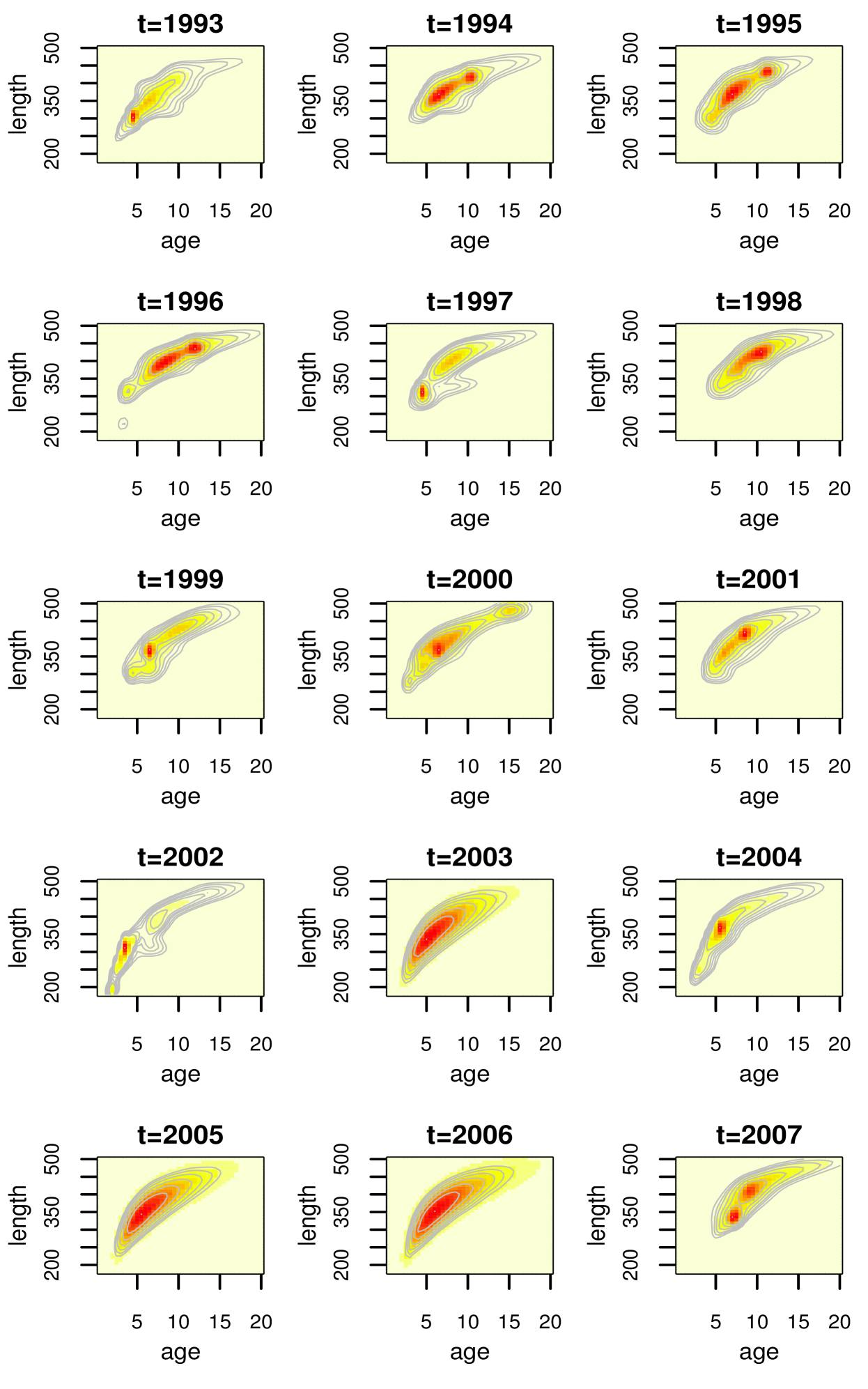
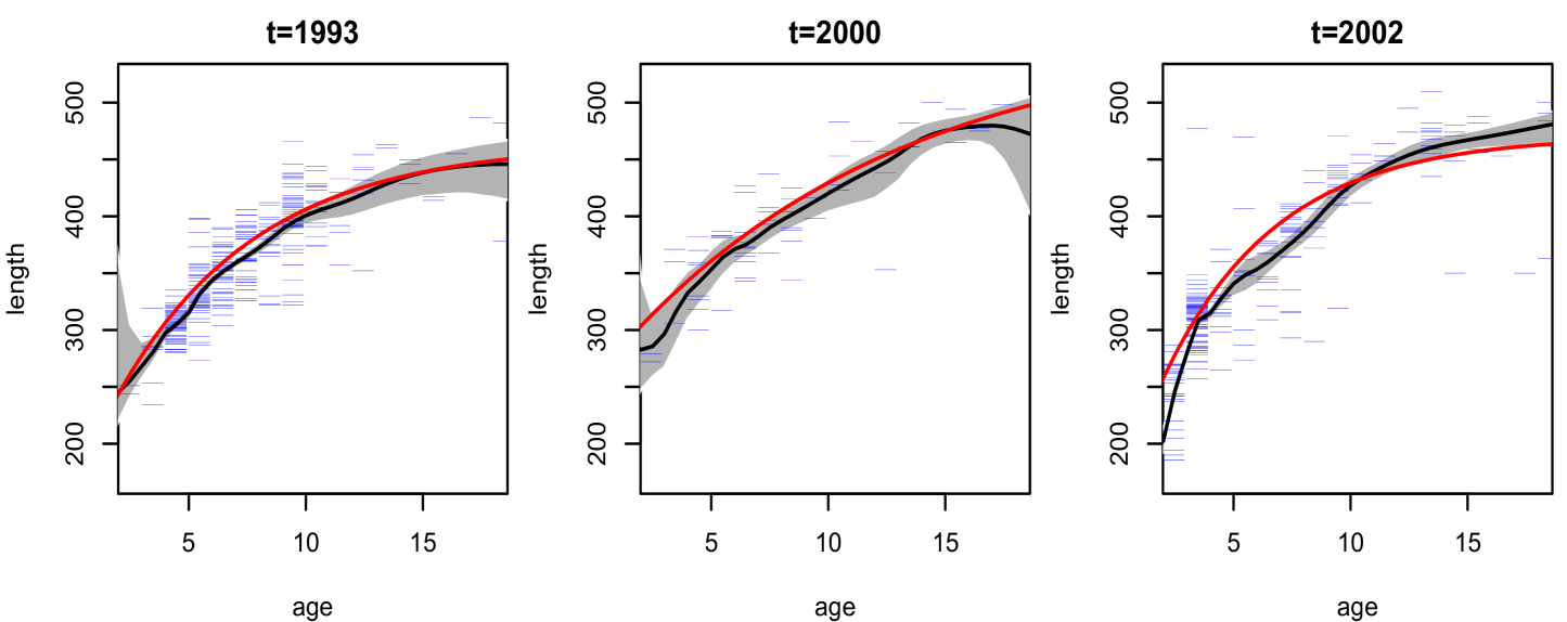
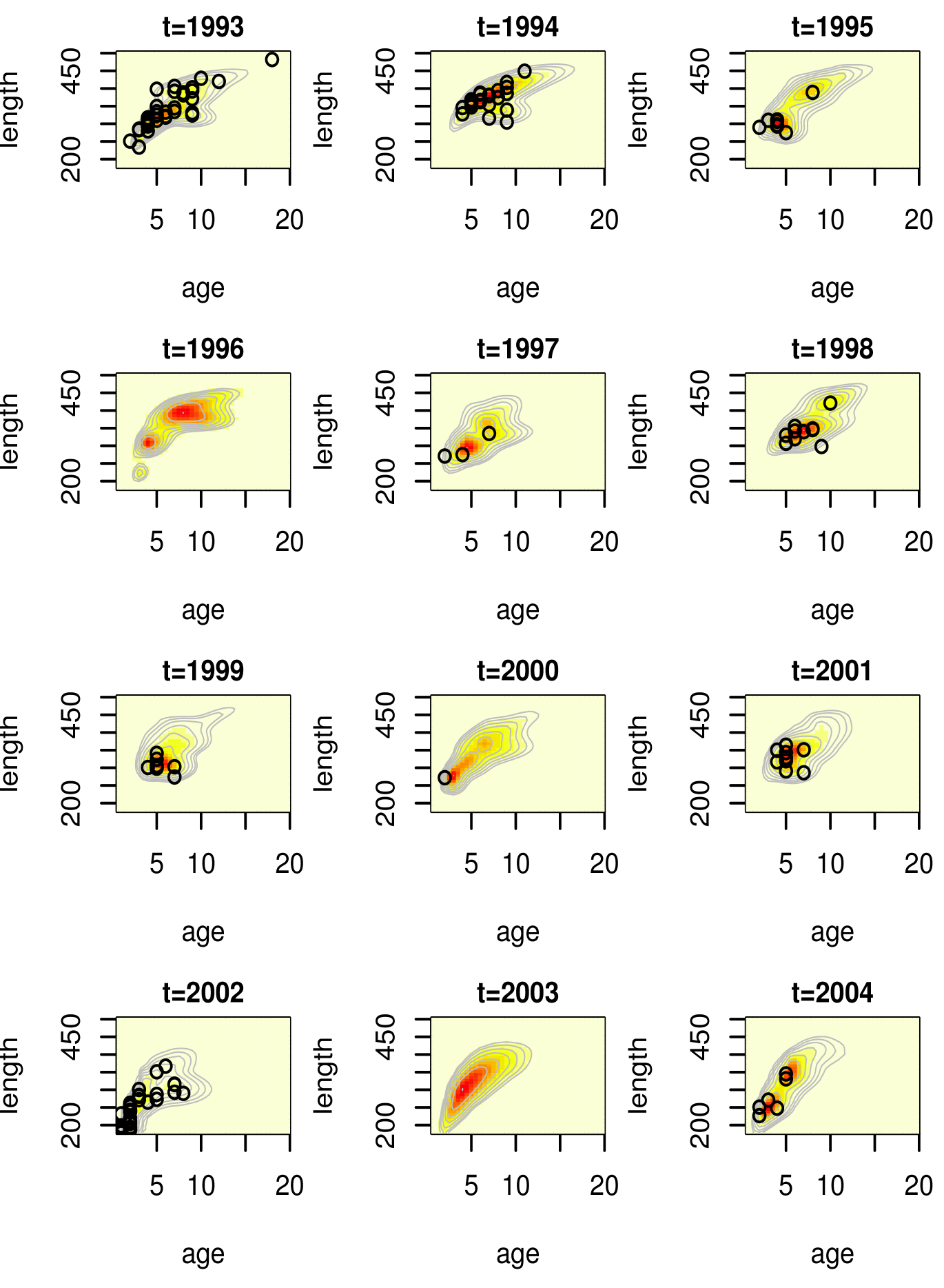
The posterior mean surfaces for the bivariate density of age and length are shown in Figure 5 for all years, including the ones (years , and ) for which data is not available. The model yields more smooth shapes for the density estimates in these years. An ellipse with a slight “banana” shape appears at each year, though some nonstandard features and differences across years are present. In particular, the density in year extends down farther to smaller ages and lengths; this year is unique in that it contains a very large proportion of the young fish which are present in the data. One can envision a curve going through the center of these densities, representing , for which we show posterior mean and interval bands for three years in Figure 6. The estimates from our model are compared with the von Bertalanffy growth curves for length-at-age, which are based on a particular function of age and three parameters (estimated here using nonlinear least squares). It is noteworthy that the nonparametric mixture model for the joint distribution of length and age yields estimated growth curves which are overall similar to the von Bertalanffy parametric model, with some local differences especially in year 2002. The uncertainty quantification in the growth curves afforded by the nonparametric model is important, since the attainment of unique growth curves by group (i.e. by location or cohort) is often used to suggest that the groups differ in some way, and this type of analysis should clearly take into account the uncertainty in the estimated curves.
The last year , in addition to containing few observations, is peculiar. There are no fish that are younger than age in this year, and most of the age and fish are recorded as immature, even though in all years combined, less than of age as well as age fish are immature. This year appears to be an anomaly. As there are no observations in or , and a small number of observations in which seem to contradict the other years of data, hereinafter, we report inferences only up to .
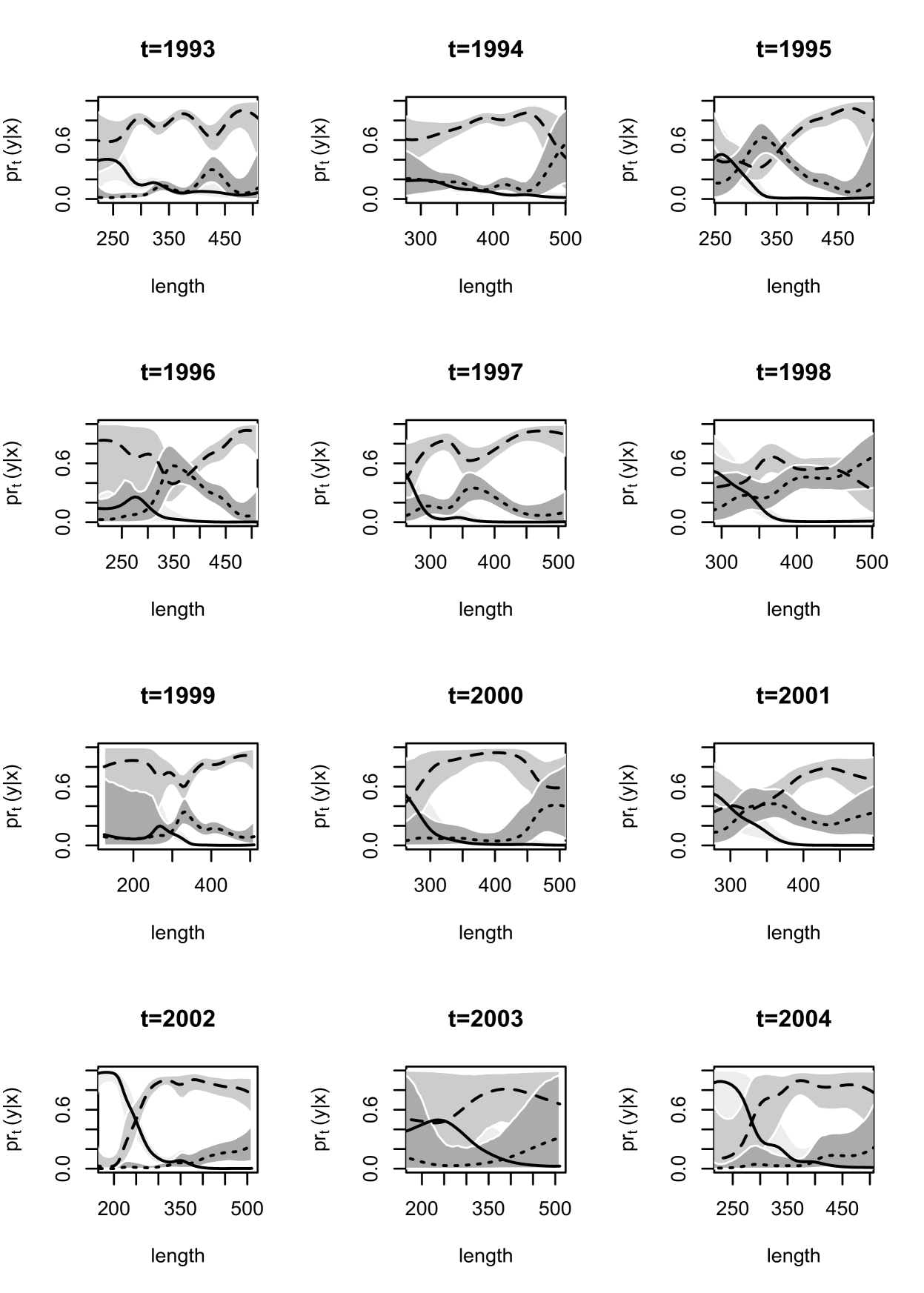
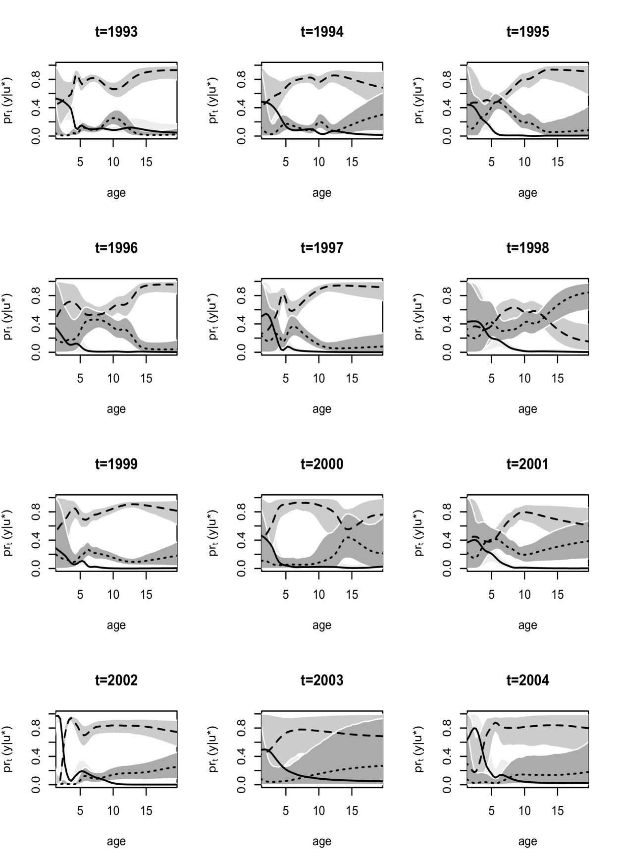
Inference for the maturation probability curves is shown over length and age in Figures 7 and 8. The probability that a fish is immature is generally decreasing over length, reaching a value near at around mm in most years. There is a large change in this probability over length in and as compared to other years, as these years suggest a probability close to for very small fish near to mm. Turning to age, the probability of immaturity is also decreasing with age, also showing differences in and in comparison to other years. There is no clear indication of a general trend in the probabilities associated with levels or . Years - and display similar behavior, with a peak in probability of post-spawning mature for moderate length values near mm, and ages -, favoring pre-spawning mature fish at other lengths and ages. The last four years - suggest the probability of pre-spawning mature to be increasing with length up to a point and then leveling off, while post-spawning is favored most for large fish. Post-spawning appears to have a lower probability than pre-spawning mature for any age at all years, with the exception of , for which the probability associated with post-spawning is very high for older fish.


The Pacific States Marine Fisheries Commission states that all Chilipepper rockfish are mature at around - years, and at size to mm. A stock assessment produced by the Pacific Fishery Management Council (Field, 2009) fitted a logistic regression to model maturity over length, from which it appears that of fish are mature around - mm. As our model does not enforce monotonicity on the probability of maturity across age, we obtain posterior distributions for the first age greater than (since biologically all fish under should be immature) at which the probability of maturity exceeds , given that it exceeds at some point. That is, for each posterior sample we evaluate over a grid in beginning at , and find the smallest value of at which this probability exceeds . Note that there were very few posterior samples for which this probability did not exceed for any age (only samples in and in ). The estimates for age at maturity are shown in the left panel of Figure 9. The model uncovers a (weak) U-shaped trend across years. Also noteworthy are the very narrow interval bands in . Recall that this year contains an abnormally large number of young fish. In this year, over half of fish age (that is, of age -) are immature, and over of age (that is, of age -) fish are mature, so we would expect the age at maturity to be above but less than , which our estimate confirms. A similar analysis is performed for length (right panel of Figure 9) suggesting a trend over time which is consistent with the age analysis.
Due to the monotonicity in the maturity probability curve in standard approaches, and the fact that age and length are treated as fixed, the point at which maturity exceeds a certain probability is a reasonable quantity to obtain in order to study the age or length at which most fish are mature. However, since we are modeling age and length, we can obtain their entire distribution at a given maturity level. These are inverse inferences, in which we study, for instance, as opposed to . It is most informative to look at age and length for immature fish, as this makes it clear at which age or length there is essentially no probability assigned to the immature category. The posterior mean estimates for are shown in Figure 10.
3.4 Model Checking
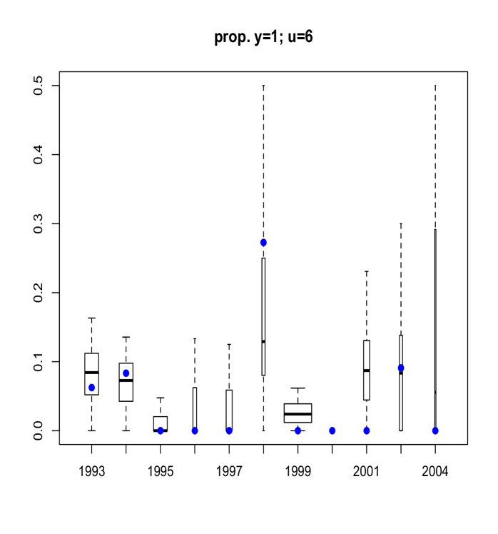
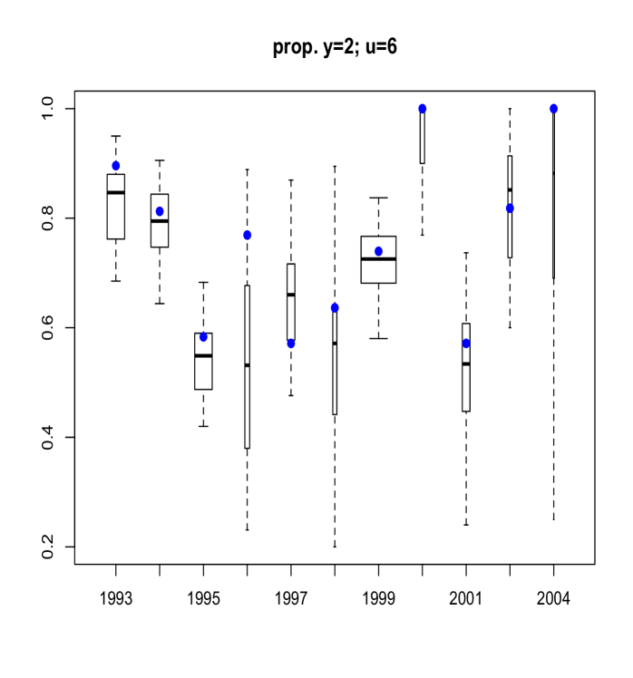
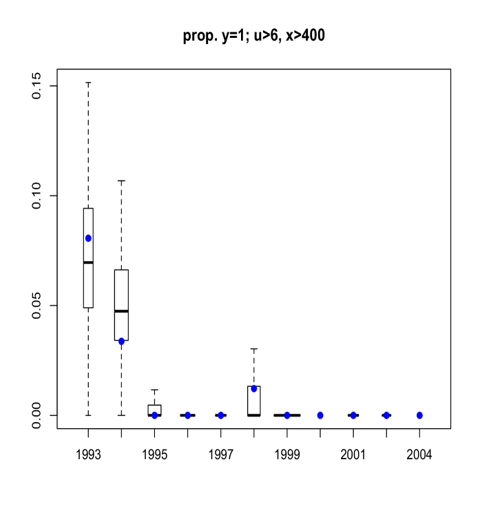
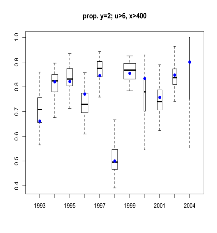
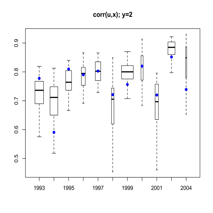
Here, we discuss results from posterior predictive model checking. In particular, we generated replicate data sets from the posterior predictive distribution, and compared to the real data using specific test quantities (Gelman et al., 2004). Using the MCMC output, we simulate replicate data sets of the same size as the original data. We then choose some test quantity, , and for each replicate data set at time , determine the value of the test quantity and compare the distribution of test quantities with the value computed from the actual data. To obtain Figure 11 we computed, for each replicate sample, the proportion of age fish that were of maturity levels and . Boxplots of these proportions are shown, with the actual proportions from the data indicated as blue points. The width of each box is proportional to the number of age fish in that year. Figure 12 refers to fish of at least age with length larger than mm. Finally, Figure 13 plots the sample correlation of length and age for fish of maturity level . The results reported in Figures 11, 12 and 13 suggest that the model is predicting data which is very similar to the observed data in terms of practically important inferences.
Although results are not shown here, we also studied residuals with cross-validation, randomly selecting of the observations in each year and refitting the model, leaving out these observations. We obtained residuals for each observation which was left out. There was no apparent trend in the residuals across covariate values, that is, no indication that we are systematically under or overestimating fish maturity of a particular length and/or age.
4 Discussion
The methods developed for dynamic ordinal regression are widely applicable to modeling mixed ordinal-continuous distributions indexed in discrete time. At any particular point in time, the DP mixture representation for the latent response-covariate distribution is retained, enabling flexible inference for a variety of functionals, and allowing standard posterior simulation techniques for DP mixture models to be utilized.
In contrast to standard approaches to ordinal regression, the model does not force specific trends, such as monotonicity, in the regression functions. We view this as an attribute in most settings. Nevertheless, in situations in which it is believed that monotonicity exists, we must realize that the data will determine the model output, and may not produce strictly monotonic relationships. In the fish maturity example, it is generally accepted that monotonicity exists in the relationship between maturity and age or length. Although our model does not enforce this, the inferences generally agree with what is expected to be true biologically. Our model is also extremely relevant to this setting, as the covariates age and length are treated as random, and the ordinal nature of recorded age is accounted for using variables which represent underlying continuous age. The set of inferences that are provided under this framework, including estimates for length as a function of age, make this modeling approach powerful for the particular application considered, as well as related problems.
While year of sampling was considered to be the index of dependence in this analysis, an alternative is to consider cohort as an index of dependence. All fish born in the same year, or the same age in a given year, represent one cohort. Grouping fish by cohort rather than year of record should lead to more homogeneity within a group, however there are also some possible issues since fish will generally be younger as cohort index increases. This is a consequence of having a particular set of years for which data is collected, i.e., the cohort of fish born in can not be older than if data collection stopped in . Due to complications such as these, combined with exploration of the relationships within each cohort, we decided to treat year of data collection as the index of dependence, but cohort indexing could be more appropriate in other analyses of similar data structures.
The proposed modeling approach could also be useful in applications in finance. One such example arises in the analysis of price changes of stocks. In the past, stocks traded on the New York Stock Exchange were priced in eighths, later moved to sixteenths, and corporate bonds still trade in eighths. In analyzing price changes of stocks which are traded in fractions, it is inappropriate to treat the measurements as continuous, particularly if the range of values is not very large (e.g., Müller and Czado, 2009). The price changes should be treated with a discrete response model, and the possible responses are ordered, ranging from a large negative return to a large positive return. One possible analysis may involve modeling the monthly returns as a function of covariates such as trade volume, and must take into account the ordinal nature of the responses. In addition, the distribution of returns in a particular month is likely correlated with the previous month, and the regression relationships must be allowed to be related from one month to the next. In finance as well as environmental science, empirical distributions may exhibit non-standard features which require more general methods, such as the nonparametric mixture model developed here.
References
- Bobko and Berkeley (2004) Bobko, S. and Berkeley, S. (2004), “Maturity, ovarian cycle, fecundity, and age-specific parturition of black rockfish (Sebastes melanops),” Fisheries Bulletin, 102, 418–429.
- Boes and Winkelmann (2006) Boes, S. and Winkelmann, R. (2006), “Ordered Response Models,” Advances in Statistical Analysis, 90, 165–179.
- Clark (1991) Clark, W. (1991), “Groundfish exploitation rates based on life history parameters,” Canadian Journal of Fisheries and Aquatic Sciences, 48, 734–750.
- De Iorio et al. (2004) De Iorio, M., Müller, P., Rosner, G., and MacEachern, S. (2004), “An ANOVA Model for Dependent Random Measures,” Journal of the American Statistical Association, 99, 205–215.
- DeYoreo (2014) DeYoreo, M. (2014), “A Bayesian Framework for Fully Nonparametric Ordinal Regression,” Ph.D. thesis, University of California, Santa Cruz.
- DeYoreo and Kottas (2014a) DeYoreo, M. and Kottas, A. (2014a), “Bayesian Nonparametric Modeling for Multivariate Ordinal Regression,” arXiv:1408.1027, stat.ME.
- DeYoreo and Kottas (2014b) — (2014b), “A Fully Nonparametric Modeling Approach to Binary Regression,” arXiv:1404.5097, stat.ME.
- Di Lucca et al. (2013) Di Lucca, M., Guglielmi, A., Muller, P., and Quintana, F. (2013), “Bayesian Dynamic Density Estimation,” A Simple Class of Bayesian Nonparametric Autoregressive Models, 8, 63–88.
- Dunson and Park (2008) Dunson, D. and Park, J. (2008), “Kernel Stick-breaking Processes,” Biometrika, 95, 307–323.
- Field (2009) Field, J. (2009), “Status of the Chilipepper rockfish, Sebastes Goodei, in 2007,” Tech. rep., Southwest Fisheries Science Center.
- Gelfand et al. (2005) Gelfand, A., Kottas, A., and MacEachern, S. (2005), “Bayesian Nonparametric Spatial Modeling with Dirichlet Process Mixing,” Journal of the American Statistical Association, 100, 1021–1035.
- Gelman et al. (2004) Gelman, A., Carlin, J., Stern, H., and Rubin, D. (2004), Bayesian Data Analysis, Chapman and Hall/CRC.
- Griffin and Steel (2006) Griffin, J. and Steel, M. (2006), “Order-based Dependent Dirichlet Processes,” Journal of the American Statistical Association, 101, 179–194.
- Hannah et al. (2009) Hannah, R., Blume, M., and Thompson, J. (2009), “Length and age at maturity of female yelloweye rockfish (Sebastes rubberimus) and cabezon (Scorpaenichthys marmoratus) from Oregon waters based on histological evaluation of maturity,” Tech. rep., Oregon Department of Fish and Wildlife.
- Ishwaran and James (2001) Ishwaran, H. and James, L. (2001), “Gibbs Sampling Methods for Stick-breaking Priors,” Journal of the American Statistical Association, 96, 161–173.
- MacEachern (1999) MacEachern, S. (1999), “Dependent Nonparametric Processes,” in ASA Procedings of the Section on Bayesian Statistical Science, pp. 50–55.
- MacEachern (2000) — (2000), “Dependent Dirichlet processes,” Tech. rep., The Ohio State University Department of Statistics.
- McKenzie (1985) McKenzie, E. (1985), “An Autoregressive Process for Beta Random Variables,” Management Science, 31, 988–997.
- Morgan and Hoenig (1997) Morgan, M. and Hoenig, J. (1997), “Estimating Maturity-at-Age from Length Stratified Sampling,” Journal of Northwest Atlantic Fisheries Science, 21, 51–63.
- Müller and Czado (2009) Müller, G. and Czado, C. (2009), “Stochastic Volatility Models for Ordinal Valued Time Series with Application to Finance,” Statistical Modeling, 9, 69–95.
- Müller et al. (1996) Müller, P., Erkanli, A., and West, M. (1996), “Bayesian Curve Fitting Using Multivariate Normal Mixtures,” Biometrika, 83, 67–79.
- Nieto-Barajas et al. (2012) Nieto-Barajas, L., Müller, P., Ji, Y., Lu, Y., and Mills, G. (2012), “A Time-Series DDP for Functional Proteomics Profiles,” Biometrics, 68, 859–868.
- Rodriguez and Dunson (2011) Rodriguez, A. and Dunson, D. (2011), “Nonparametric Bayesian models through probit stick-breaking processes,” Bayesian Analysis, 6, 145–177.
- Rodriguez and ter Horst (2008) Rodriguez, A. and ter Horst, E. (2008), “Bayesian Dynamic Density Estimation,” Bayesian Analysis, 3, 339–366.
- Rubin (1976) Rubin, D. (1976), “Inference and Missing Data,” Biometrika, 63, 581–592.
- Sethuraman (1994) Sethuraman, J. (1994), “A Constructive Definition of Dirichlet Priors,” Statistica Sinica, 4, 639–650.
- Taddy (2010) Taddy, M. (2010), “Autoregressive Mixture Models for Dynamic Spatial Poisson Processes: Application to Tracking the Intensity of Violent Crime,” Journal of the American Statistical Association, 105, 1403–1417.
- Xiao et al. (2015) Xiao, S., Kottas, A., and Sansó, B. (2015), “Modeling for seasonal marked point processes: An analysis of evolving hurricane occurrences,” The Annals of Applied Statistics, 9, 353–382.
Appendix A Properties of the DDP Prior Model
Here, we provide derivations of the various correlations associated with the DDP prior, as given in Section 2.3.
Autocorrelation of
Since the process is stationary with at any time , and . We also have
| (A.1) |
using the definition of the process in (2). The first expectation can be obtained through the moment generating function of , which is given by , for . Hence, for , we obtain . Regarding the second expectation, note that , with a covariance matrix with diagonal elements equal to 1 and off-diagonal elements equal to . Integration results in . The correlation in (3) results by combining the terms above with the expressions for and .
Autocorrelation of DP weights
First, . Since the are independent across , and , we obtain . Similarly, , from which obtains.
Since , and is independent of , for any , we can write
The required expectations in the above equation can be obtained from (A.1) for , such that . Combining the above expressions yields the covariance in (4).
Autocorrelation of consecutive distributions
The DDP prior model implies at any a prior for , where the are i.i.d. from a distribution on . Hence, for any measurable subset , we have , and .
The additional expectation needed in order to obtain is , which can be written as
| (A.2) |
For the first expectation in (A.2), note that is independent of , and has been derived earlier. Moreover, since is equal to if and otherwise, . Regarding the second expectation in (A.2), we have again that and are independent. Here, , since and are independent for . The final step of the derivation involves the expectations , for . Note that, if , , and an analogous expression can be written when . Therefore, for general , can be expressed as a product of independent components, since each component comprises one or two of the random variables in and , in the latter case having the same first subscript. Thus, can be developed through products of expectations of the form and , which have been obtained earlier.
Appendix B Posterior Simulation Details
We derive the posterior full conditionals and provide updating strategies for many of the parameters of the hierarchical model in Section 3.2.
Updating the weights
The full conditional for is given by
Write , where , i.e., the number of observations at time assigned to component . Filling in the form for gives
The full conditional for each , , is therefore
giving
We use a slice sampler to update , with the following steps:
-
•
Draw , for
-
•
Draw , restricted to the lie in the interval . Solving for in each of these equations gives , for . Therefore, if for all , then has no restrictions, and is therefore sampled from a normal distribution. Otherwise, if for some , then . This then requires sampling from a normal distribution, restricted to the intervals , and .
In the second step above, we may have to sample from a normal distribution, restricted to two disjoint intervals. The resulting distribution is therefore a mixture of two truncated normals, with probabilities determined by the (normalized) probability the normal assigns to each interval. These truncated normals both have mean and variance , and each mixture component has equal probability.
The full conditional for each , , , is proportional to
Each , , and , can therefore be sampled with a slice sampler:
-
•
Draw .
-
•
Draw , restricted to , giving .
In the second step above, we will again either sample from a single normal or a mixture of truncated normals, where each normal has the same mean and variance, but the truncation intervals differ. Since the mean of this normal is not zero, the weights assigned to each truncated normal are not the same. The unnormalized weight assigned to the normal which places positive probability on is given by , where is the CDF of the normal for given in the second step. The unnormalized weight given to the component which places positive probability on is given by .
The full conditionals for and are slightly different. The full conditional for is
For , we have:
which is proportional to
The slice samplers for and are therefore implemented in the same way as for , except the normals which are sampled from have different means and variances.
Updating
The full conditional for is
Therefore, with , we have
The parameter can be sampled using a Metropolis-Hastings algorithm. In particular we work with , and use a normal proposal distribution centered at the log of the current value of .
Updating
The full conditional for the AR parameter is
We assume or , and apply a Metropolis-Hastings algorithm to sample or , respectively, using a normal proposal distribution.
Updating
The updates for are , with and given by:
-
•
For , if , then the update for has and
-
•
For , if , then the update for has and
-
•
for , if , then the update for has , and
-
•
for , if , then the update for has and
-
•
for , if , then the update for has , and
-
•
for , if , then the update for has and
Updating
The posterior full conditional for is proportional to . When , is drawn from .