Modeling Gamma-ray burst Afterglow observations with an Off-axis Jet emission

N. Fraija^1†, A. Galvan-Gamez¹, B. Betancourt Kamenetskaia^2,3, M.G. Dainotti^4,5, S. Dichiara ^6,7, P. Veres⁸, R. L. Becerra⁹ and A. C. Caligula do E. S. Pedreira¹ ¹ Instituto de Astronomía, Universidad Nacional Autónoma de México, Circuito Exterior, C.U., A. Postal 70-264, 04510 Cd. de México, México. ² LMU Physics Department, Ludwig Maxmillians University,Theresienstr. 37, 80333 Munich, Germany ³ TUM Physics Department, Technical University of Munich, James-Franck-Str, 85748 Garching, Germany ⁴ National Astronomical Observatory of Japan, Division of Science, Mitaka, 2-chome ⁵ Space Science Institute, Boulder, Colorado ⁶ Department of Astronomy, University of Maryland, College Park, MD 20742-4111, USA ⁷ Astrophysics Science Division, NASA Goddard Space Flight Center, 8800 Greenbelt Rd, Greenbelt, MD 20771, USA ⁸ Center for Space Plasma and Aeronomic Research (CSPAR), University of Alabama in Huntsville, Huntsville, AL 35899, USA ⁹ Instituto de Ciencias Nucleares, Universidad Nacional Autónoma de México, Apartado Postal 70-264, 04510 México, CDMX, Mexico

\dagger

nifraija@astro.unam.mx

Abstract

Gamma-ray bursts (GRBs) are fascinating extragalactic objects. They represent a fantastic opportunity to investigate unique properties not exhibited in other sources. Multi-wavelength afterglow observations from some short- and long-duration GRBs reveal an atypical long-lasting emission that evolves differently from the canonical afterglow light curves favoring the off-axis emission. We present an analytical synchrotron afterglow scenario, and the hydrodynamical evolution of an off-axis top-hat jet decelerated in a stratified surrounding environment. The analytical synchrotron afterglow model is shown during the coasting, deceleration (off- and on-axis emission), and the post-jet-break decay phases, and the hydrodynamical evolution is computed by numerical simulations showing the time evolution of the Doppler factor, the half-opening angle, the bulk Lorentz factor, and the deceleration radius. We show that numerical simulations are in good agreement with those derived with our analytical approach. We apply the current synchrotron model and describe successfully the delayed non-thermal emission observed in a sample of long and short GRBs with evidence of off-axis emission. Furthermore, we provide constraints on the possible afterglow emission by requiring the multi-wavelength upper limits derived for the closest Swift-detected GRBs and promising gravitational-wave events.

Subject headings:

Gamma-ray bursts: individual — Stars: neutron — Physical data and processes: acceleration of particles — Physical data and processes: radiation mechanism: nonthermal — ISM: general - magnetic fields

1. Introduction

Gamma-ray bursts (GRBs) are among the most powerful transient events in the Universe. These events are detected as brief, non-repeating flashes in the gamma-rays bands. Depending on the burst duration (from milliseconds to thousands of seconds), GRBs are commonly classified as short (sGRBs) and long GRBs (lGRBs) (Kouveliotou et al., 1993). A lGRB is associated with the core collapse (CC) of dying massive star (Woosley, 1993; Galama et al., 1998) that lead to supernova (SNe; Bloom et al., 1999; Woosley & Bloom, 2006). At the same time, a sGRB is linked with the merger of a neutron star (NS) with a black hole (BH, Narayan et al., 1992) or two NSs (Duncan & Thompson, 1992; Usov, 1992; Thompson, 1994; Metzger et al., 2011) as demonstrated by the historical gravitational-wave (GW) and electromagnetic detections of the GW170817 event (Abbott et al., 2017a).

On August 17, 2017, the joint detection of two messengers of the fusion of two NSs was achieved for the first time: the GW event (GW170817) by the Laser Interferometer Gravitational-Wave Observatory (LIGO) and VIRGO (Abbott et al., 2017a; von Kienlin et al., 2017) and the associated low-luminosity burst, GRB 170817A by the Fermi Gamma-ray Space Telescope (von Kienlin et al., 2017) and The INTErnational Gamma-Ray Astrophysics Laboratory (INTEGRAL; Savchenko et al., 2017). The results of this joint observation confirmed that NS fusion is a progenitor of sGRBs (Abbott et al., 2017). The association of GW170817A with the near host galaxy NGC 4993, located at a redshift of $z\simeq 0.01$ (Coulter et al., 2017; Margutti et al., 2017b) suggested the presence of a local population of low-luminosity bursts following the merger of two NSs (Abbott et al., 2017). Immediately, GRB 170817A was followed up by large observational campaigns covering the X-ray (Troja et al., 2017; Margutti et al., 2018; Alexander et al., 2018; D’Avanzo et al., 2018; Margutti et al., 2017a; Haggard et al., 2018), optical (Lyman et al., 2018; Margutti et al., 2018) and radio (Abbott et al., 2017b; Mooley et al., 2017; Dobie et al., 2018; Troja et al., 2017) bands, among others. In order to describe the delayed multi-wavelength observations in timescales of days, synchrotron external-shock models radiated from off-axis top-hat jets (Troja et al., 2017; Margutti et al., 2017b; Ioka & Nakamura, 2017; Alexander et al., 2017; Fraija et al., 2019a, b), radially stratified ejecta (Mooley et al., 2017; Fraija et al., 2019c; Hotokezaka et al., 2018) and structured jets (Kasliwal et al., 2017; Lazzati et al., 2017) were proposed. Later, analyses performed by Burns et al. (Burns et al., 2018) and other authors (Troja et al., 2018; Burns et al., 2018; Fong et al., 2016) showed that GRB 150101B exhibits characteristics similar to GRB 170817A, in terms of its two-component structure and an undetected afterglow in a timescale of days followed by bright X-ray emission. Similar features in the multi-wavelength afterglow have been found in GRB 080503 (Perley et al., 2009), GRB 140903A (Troja et al., 2016) and GRB 160821B (Lü et al., 2017; Stanbro & Meegan, 2016). On the other hand, several searches for afterglow emission around the closest bursts ( $\lesssim 200\,{\rm Mpc}$ ) reported by the Burst Alert Telescope (BAT) instrument onboard the Neil Gehrels Swift Observatory (Dichiara et al., 2020) and the GW events by Advanced LIGO and Advanced VIRGO detectors (Abbott et al., 2021; The LIGO Scientific Collaboration et al., 2021) have been performed without successful, but setting multi-wavelength upper limits.

The density profile of the medium surrounding a burst has been addressed previously in different contexts. For instance, for the case of SNe, Chevalier (1982) studied the interaction of an adiabatic flow in a circumstellar density profile for Type II SNe of the form $\propto r^{-2}$ . Ever since, subsequent authors have adopted this proposal for modeling the circumstellar medium, and it has even been applied in the research of different SN types. Examples of such studies are those by Blondin et al. (1996), Soderberg et al. (2006), Kotak et al. (2004), and Chevalier (1984), among others. Nevertheless, a generalization of this power law has also been considered. A later study, Moriya & Tominaga (2012) showed that the diversity might explain the spectral diversity of Type II luminous SNe in the density slope of the surrounding dense wind. To this effect, they proposed a wind density structure in the form $\propto r^{-k}$ . They noticed that the ratio of the diffusion timescale in the optically thick region of the wind and the shock propagation timescale after the shock breakout strongly depends on the stratification parameter $k$ , which led to differences in the spectral SN evolution. On the other hand, the requirement of a stratified environment condition has been proposed in some cases for modeling the multi-wavelength afterglows, such as in work by Yi et al. (2013). The authors analyzed more than one dozen GRBs and concluded that the circumburst environment could be neither a homogeneous nor a stellar-wind medium but something in between, with a general density distribution with a stratification parameter in the range $0.4\leq k\leq 1.4$ . A more recent example of an analysis that links SN and GRB emission with a stratified environment is the one by Izzo et al. (2020), in which the authors studied SN 2020bvc. They found an excellent agreement with the GRB-associated, broad-lined Ic SN 1998bw; thus, it was categorized as a young broad-lined Ic SN. They also noted that its X-ray light curve was consistent with simulations of an off-axis GRB afterglow in a stratified medium with $k=1.5$ ; thus, this event represented the first case of an off-axis GRB discovered via its associated SN. It was later argued by Ho et al. (2020b), however, that such a model would predict an 8.5 GHz radio light curve several orders of magnitude more luminous than their measurements. Nevertheless, they stated that an off-axis jet could not be ruled out, and future radio observations would be needed.

In this work, we extend the analytical synchrotron afterglow scenario of the off-axis top-hat jet used to describe the multi-wavelength afterglow observations in GRB 170817A (see Fraija et al., 2019b) adding several ingredients. Here we consider i) the circumburst external medium as stratified with a profile density $\propto r^{-k}$ with ${\rm k}$ in the range of $0\leq k<3$ , ii) the synchrotron radiation in self-absorption regime, iii) the afterglow emission during the transition from off-axis to on-axis before the lateral expansion phase (relativistic phase), iv) the hydrodynamical evolution computed by numerical simulations and v) a fraction of electrons accelerated by the shock front. We apply the current model to describe the delayed non-thermal emission observed in GRB 080503, GRB 140903A, GRB 150101B, GRB 160821B, and SN 2020bvc, and to provide constraints on the possible afterglow emission using multi-wavelength upper limits associated with the closest Swift-detected sGRBs and the promising GW events. This paper is arranged as follows: Section 2 presents the analytical synchrotron scenario and an hydrodynamical evolution of an off-axis top-hat jet decelerated in a stratified surrounding environment. In Section 3, we apply the proposed analytical model to describe the multi-wavelength observations of a sample of bursts and provide constraints to other ones. In Section 4, we present our conclusions.

2. Off-axis top hat model

2.1. Radiative model

Accelerated electrons in forward-shock models are distributed in accordance with their Lorentz factors ( $\gamma_{e}$ ) and are described by the electron power index $p$ as $N(\gamma_{e})\,d\gamma_{e}\propto\gamma_{e}^{-p}\,d\gamma_{e}$ for $\gamma_{m}\leq\gamma_{\rm e}$ , where $\gamma_{m}=m_{\rm p}/m_{\rm e}g(p)\varepsilon_{\rm e}(\Gamma-1)\zeta^{-1}_{e}$ is the minimum electron Lorentz factor with $\Gamma$ is the bulk Lorentz factor, $m_{\rm p}$ and $m_{\rm e}$ the proton and electron mass, $\varepsilon_{\rm e}$ is the fraction of energy given to accelerate electrons, $\zeta_{e}$ denotes the fraction of electrons that were accelerated by the shock front (Fan & Piran, 2006) and $g(p)=\frac{p-2}{p-1}$ . The comoving of the magnetic field strength in the blastwave $B^{\prime 2}/(8\pi)=\varepsilon_{B}e$ is derived from the energy density $e=[(\hat{\gamma}\Gamma+1)/(\hat{\gamma}-1)](\Gamma-1)n(r)m_{p}c^{2}$ with $\hat{\gamma}$ the adiabatic index (Huang et al., 1999) and its respective fraction given to magnetic field ( $\varepsilon_{B}$ ). Hereafter, we adopt the unprimed and prime terms to refer them in the observer and comoving frames, respectively. The term $\hat{\gamma}$ is the adiabatic index and $n(r)=A_{\rm k}\,r^{\rm-k}=\frac{\dot{M}_{\rm W}}{4\pi v_{\rm W}}\,r^{\rm-k}$ , where $v_{\rm W}$ is the wind velocity and $\dot{M}_{\rm W}$ is the mass-loss rate. The sub-index ${\rm k}$ lies in the range $0\leq k\leq 3$ , with ${\rm k=0}$ the constant-density medium ( $A_{\rm 0}=n$ ), and ${\rm k=2}$ the stellar wind ejected by its progenitor ( $A_{\rm 2}\simeq A_{\rm W}\,3\times 10^{35}{\rm cm}^{-1}$ ) where $A_{\rm W}$ is the density parameter. The cooling electron Lorentz factor is $\gamma_{\rm c}=(6\pi m_{e}c/\sigma_{T})(1+Y)^{-1}\Gamma^{-1}B^{\prime-2}t^{-1}$ , where $\sigma_{T}$ is the cross-section in the Thomson regime and $Y$ is the Compton parameter (Sari & Esin, 2001; Wang et al., 2010). The synchrotron spectral breaks and the synchrotron radiation power per electron in the comoving frame are given by $\nu^{\prime}_{\rm i}=q_{e}/(2\pi m_{e}c)\gamma^{2}_{\rm i}B^{\prime}$ and $P^{\prime}_{\nu^{\prime}_{m}}\simeq\sqrt{3}q_{e}^{3}/(m_{e}c^{2})B^{\prime}$ , respectively, with hereafter the subindex ${\rm i=m}$ and ${\rm c}$ for the characteristic and cooling break, and the constants $q_{e}$ and $c$ the elementary charge and the speed of light, respectively (e.g., see Sari et al., 1998; Fraija, 2015). The synchrotron spectral breaks in the self-absorption regime are derived from $\nu^{\prime}_{\rm a,1}=\nu^{\prime}_{\rm c}\tau^{\frac{3}{5}}_{0,m}$ , $\nu^{\prime}_{\rm a,2}=\nu^{\prime}_{\rm m}\tau^{\frac{2}{p+4}}_{0,m}$ and $\nu^{\prime}_{\rm a,3}=\nu^{\prime}_{\rm m}\tau^{\frac{3}{5}}_{0,c}$ with the optical depth given by $\tau_{0,i}\simeq\frac{5}{3-k}\frac{q_{e}n(r)r}{B^{\prime}\gamma^{5}_{\rm i}}$ with $r$ the shock radius (Panaitescu & Mészáros, 1998). Considering the total number of emitting electrons $N_{e}=(\Omega/4\pi)\,n(r)\frac{4\pi}{3-k}r^{3}$ and also taking into account the transformation laws for the solid angle ( $\Omega=\Omega^{\prime}/\delta^{2}_{D}$ ), the radiation power ( $P_{\nu_{m}}=\delta_{D}/(1+z)P^{\prime}_{\nu^{\prime}_{m}}$ ) and the spectral breaks ( $\nu_{\rm i}=\delta_{D}/(1+z)\nu^{\prime}_{\rm i}$ ), the maximum flux given by synchrotron radiation is

F_{\rm\nu,max}=\frac{(1+z)^{2}\delta^{3}_{D}}{4\pi d_{z}^{2}}N_{e}P^{\prime}_{\nu^{\prime}_{m}}\,,

(1)

where $d_{\rm z}=(1+z)\frac{c}{H_{0}}\int^{z}_{0}\,\frac{d\tilde{z}}{\sqrt{\Omega_{\rm M}(1+\tilde{z})^{3}+\Omega_{\Lambda}}}$ (Weinberg, 1972) is the luminosiy distance, $r=\delta_{D}/(1+z)\Gamma\beta ct$ is the shock radius, and $\delta_{D}=\frac{1}{\Gamma(1-\mu\beta)}$ is the Doppler factor with $\mu=\cos\Delta\theta$ , $\beta=v/c$ with $v$ the velocity of the material, and $\Delta\theta=\theta_{\rm obs}-\theta_{\rm j}$ is given by the viewing angle ( $\theta_{\rm obs}$ ) and the half-opening angle of the jet ( $\theta_{\rm j}$ ). We assume for the cosmological constants a spatially flat universe $\Lambda$ CDM model with $H_{0}=69.6\,{\rm km\,s^{-1}\,Mpc^{-1}}$ , $\Omega_{\rm M}=0.286$ and $\Omega_{\Lambda}=0.714$ (Planck Collaboration et al., 2016).

2.2. Hydrodynamical evolution vs analytical approach

2.2.1 Hydrodynamical evolution

We consider the dynamical equations proposed by Huang et al. (1999, 2000). The dynamical evolution of the relativistic outflow into the circumburst medium can be described by

	$\displaystyle\frac{dr}{dt}$	$\displaystyle=$	$\displaystyle\beta c\Gamma\left(\Gamma+\sqrt{\Gamma^{2}-1}\right),\hskip 28.45274pt\frac{dm}{dr}=2\pi\,(1-\cos\theta_{\rm j})r^{2}nm_{p}$		(2)
	$\displaystyle\frac{d\theta_{\rm j}}{dt}$	$\displaystyle=$	$\displaystyle\frac{c_{s}}{r}(\Gamma+\sqrt{\Gamma^{2}-1}),\hskip 42.67912pt\frac{d\Gamma}{dm}=-\frac{\Gamma^{2}-1}{M_{\rm ej}+\epsilon m+2(1-\epsilon)\Gamma m}\,,$		(3)

where $c_{s}=\sqrt{\hat{\gamma}(\gamma-1)(\Gamma-1)c^{2}/\left(1+\hat{\gamma}(\Gamma-1)\right)}$ with $\hat{\gamma}\approx(4\Gamma+1)/3\Gamma$ , $M_{\rm ej}$ is the initial value of the ejected mass and $\epsilon$ is the radiative efficiency with $\epsilon=0$ in the adiabatic regime and $\epsilon=1$ in the fully radiative regime. The previous equations are consistent with the self-similar solution during the ultra-relativistic (Blandford-McKee solution; Blandford & McKee, 1976) and the Newtonian phase (Sedov-Taylor solution), respectively, and consider the beaming effect (Rhoads, 1999).

The observed quantities are integrated over the equal arrival time surface (EATS) determined by (Waxman, 1997)

t=(1+z)\int\frac{dr}{\beta\Gamma c\delta_{D}}\equiv{\rm const.}

(4)

2.2.2 Analytical approach

During the coasting phase (before the deceleration phase), the relativistic outflow is not affected by the circumburst medium, so the bulk Lorentz factor is constant $\Gamma_{\rm cp}=\Gamma_{0}$ and the radius evolves as $r=c\beta_{0}t/[(1+z)(1-\beta_{0}\mu)]$ with $\beta_{0}=\sqrt{\Gamma^{2}_{0}-1}/\Gamma_{0}$ . During the deceleration phase, the relativistic outflow transfers a large amount of its energy to the circumstellar medium driving a forward shock. Considering the adiabatic evolution of the forward shock with an isotropic equivalent-kinetic energy $E=\frac{4\pi}{3}m_{p}c^{2}A_{\rm k}r^{3}\Gamma^{2}$ (Blandford-McKee solution; Blandford & McKee, 1976) and a radial distance $r=c\beta_{\rm of}t/[(1+z)(1-\beta_{\rm of}\mu)]$ , the bulk Lorentz factor evolves as

\Gamma_{\rm of}=\left(\frac{3}{4\pi\,m_{p}c^{5-k}}\right)^{\frac{1}{2}}\,(1+z)^{-\frac{k-3}{2}}(1-\beta\cos\Delta\theta)^{-(k-3)}\,A_{\rm k}^{-\frac{1}{2}}\,E^{\frac{1}{2}}t^{\frac{k-3}{2}}\,,

(5)

with $\beta_{\rm of}=\sqrt{\Gamma^{2}_{\rm of}-1}/\Gamma_{\rm of}$ . The deceleration time scale $t_{\rm dec}$ can be defined using eq. 5. As the bulk Lorentz factor becomes $\Gamma\simeq 1/\Delta\theta$ , the observed flux becomes in our field of view. During the on-axis emission, the bulk Lorentz factor in the adiabatic regime evolves as

\Gamma_{\rm on}=\left(\frac{3}{(2c)^{5-k}\pi\,m_{p}}\right)^{\frac{1}{8-2k}}\,(1+z)^{-\frac{k-3}{8-2k}}A_{\rm k}^{-\frac{1}{8-2k}}E^{\frac{1}{8-2k}}\,t^{\frac{k-3}{8-2k}}\,,

(6)

with the radius $r\simeq 2\beta_{\rm on}\Gamma^{2}_{\rm on}ct/(1+z)$ and $\beta_{\rm on}=\sqrt{\Gamma^{2}_{\rm on}-1}/\Gamma_{\rm on}$ , before the outflow enters to the post-jet-break decay phase ( $\Gamma\simeq 1/\theta_{j}$ ). During the post-jet-break decay phase, the bulk Lorentz factor evolves as

\Gamma_{\rm le}=\left(\frac{3}{(2c)^{5-k}\pi\,m_{p}}\right)^{\frac{1}{6-2k}}\,(1+z)^{-\frac{k-3}{6-2k}}A_{\rm k}^{-\frac{1}{6-2k}}E^{\frac{1}{6-2k}}\theta_{j}^{\frac{1}{3-k}}t^{\frac{k-3}{6-2k}}\,,

(7)

with the shock’s radius and velocity given by $r\simeq 2\beta_{\rm le}\Gamma^{2}_{\rm le}ct/(1+z)$ and $\beta_{\rm le}=\sqrt{\Gamma^{2}_{\rm le}-1}/\Gamma_{\rm le}$ , respectively. We summarize the evolution of the bulk Lorentz factor as

\displaystyle\Gamma\propto\cases{t^{0},\hskip 42.67912ptt<t_{\rm dec},\cr t^{\frac{k-3}{2}},\hskip 31.2982ptt_{\rm dec}\leq t\leq t_{\rm pk},\cr t^{\frac{k-3}{8-2k}},\hskip 25.6073ptt_{\rm pk}\leq t\leq t_{\rm br},\hskip 5.69046pt\cr t^{\frac{k-3}{6-2k}}\,\hskip 34.14322ptt_{\rm br}\leq t,\hskip 5.69046pt\cr}

(8)

where the respective timescales are

$\displaystyle t_{\rm dec}$	$\displaystyle=$	$\displaystyle t_{\rm dec,0}(1+z)(1-\beta\cos\Delta\theta)^{2}A_{\rm k}^{-\frac{1}{k-3}}E^{\frac{1}{k-3}}\Gamma^{-\frac{2}{3-k}}$	(9)
$\displaystyle t_{\rm pk}$	$\displaystyle=$	$\displaystyle t_{\rm pk,0}(1+z)A_{\rm k}^{\frac{1}{k-3}}E^{-\frac{1}{k-3}}\Delta\theta^{-\frac{8-2k}{k-3}}$	(10)
$\displaystyle t_{\rm br}$	$\displaystyle=$	$\displaystyle t_{\rm br,0}(1+z)A_{\rm k}^{-\frac{1}{3-k}}E^{\frac{1}{3-k}}\theta_{\rm j}^{2}\,,$	(11)

with $t_{\rm dec,0}=(3/4\pi\,m_{p}c^{5-k})^{\frac{1}{3-k}}$ and $t_{\rm pk,0}=t_{\rm br,0}=(3/(2c)^{5-k}\pi\,m_{p})^{\frac{1}{3-k}}$ . It is worth noting that the afterglow emission enters in the observer’s field of view at $t_{\rm pk}$ . For instance, the bulk Lorentz factor in a constant-density medium evolves as first $\propto t^{0}$ (Sari & Piran, 1999), then $t^{-\frac{3}{2}}$ (Nakar & Piran, 2018; Fraija et al., 2019b), moreover $t^{-\frac{3}{8}}$ (Sari et al., 1998), and finally $t^{-\frac{1}{2}}$ (Sari et al., 1999), as expected.

The minimum and cooling electron Lorentz factors, the spectral breaks, the maximum flux and the synchrotron light curves during the coasting, deceleration (off- and on-axis) and post-jet-break decay phases are shown in Appendix A and Tables 1, 2 and 3.

2.3. Comparison of our model with previous simulations

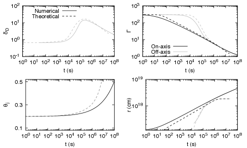
Figure 1 presents examples of the time evolution of the Doppler factor, the half-opening angle, the bulk Lorentz factor, and the deceleration radius, all in a constant circumburst medium ( $k=0$ ). The solid lines characterize the numerical simulations, while the dashed lines stand-in for the theoretical approximations, which are detailed in Appendix A. Lines in black color corresponds to quantities observed off-axis and in gray color the ones observed on-axis.

For the case of $\delta_{D}$ , the upper left panel shows an excellent agreement between the simulations and the model at early times up to $t_{\rm obs}\approx 10^{2}\,{\rm s}$ . After this point, there are very slight variations between both solutions, specifically in the steepness of the rise and fall of this quantity. The numerical simulation predicts a sharper peak, while the theoretical approximation anticipates a wider profile. Despite this slight difference, both curves drop in parallel, showing that their delinquent behavior follows the same power law. In the case of the half-opening angle $\theta_{\rm j}$ (lower left panel), as in the case of $\delta_{D}$ , the early time evolution is the same between both curves. The difference in their behavior is first made apparent at $t_{\rm obs}\approx 10^{2}\,{\rm s}$ . At this time, the theoretical solution presents a faster rise than the simulation. The initial variation between both curves keeps increasing and becomes substantial at times $\geq 10^{6}\,{\rm s}$ .

The upper right panel compares the bulk Lorentz factors when the emission is off- and on-axis. For the off-axis case, the same features mentioned in the last two panels are repeated, namely perfect agreement at early times and variations at late times. However, the on-axis emission is different as there are slight differences initially, but both solutions tend to be the same as time progresses. Finally, the right panel on the bottom presents the shock’s radius for the on- and off-axis cases. For the on-axis curves, the simulation and the theoretical approximation differ early, but they unite late. There is also a difference in their shapes at the beginning, as the theoretical curve is a straight line, which corresponds to a single power law. At the same time, the simulation shows that there is a transition from a flatter curve to a steeper one. The case of the off-axis emission presents similar differences. In general, the simulation and the theoretical variables exhibited in Figure 1 are in good agreement.

2.4. Analysis and description of the synchrotron light curves

The analytical synchrotron afterglow model during the coasting, deceleration (off- and on-axis emission), and the post-jet-break decay phases are shown in Appendix A. Table 1 shows the evolution of the synchrotron light curves, and Table 2 shows closure relations of synchrotron radiation as a function of $k$ during the coasting, deceleration (off- and on-axis emission), and the post-jet-break decay phases in the stratified environment. We can note in both tables that a break is expected around the transition time between fast- and slow-cooling regimes during the deceleration phase when the afterglow emission is seemed off-axis, but not during another phase.

Figures 2 and 3 show the predicted synchrotron light curves produced by the deceleration of the off-axis top-hat jet in the circumburst medium described by a density profile with ${\rm k}=0$ , $1.0$ , $1.5$ and $2.0$ , respectively. Panels from top to bottom correspond to radio wavelength at 6 GHz, optical at R-band and X-rays at 1 keV for typical values of GRB afterglow.¹¹1 $E=10^{54}\,{\rm erg}$ , $\varepsilon_{\rm B}=10^{-4}$ , $\varepsilon_{\rm e}=10^{-1}$ , $\zeta_{e}=1.0$ and $d_{z}=1\,{\rm Gpc}$ . Henceforth, we adopt the convention $Q_{\rm x}=Q/10^{\rm x}$ in cgs units for all variables except angles. For angles, we adopt the convention $Q_{\rm x}=Q/{\rm x}$ in degrees. These figures display that regardless of the viewing angle, the X-ray, optical, and radio fluxes increase gradually, reach the maximum value, and finally, they begin to decrease. It can be observed that as the viewing angle increases, the maximum value moves to later times. For the chosen parameters, in most cases the maximum value lies in the range $(10^{-1}-10^{2})\,{\rm days}$ for $0\,\leq\theta_{\rm obs}\leq 60\,{\rm deg}$ . This is different, however, when the medium is like a stellar wind, as the right column of Figure 3 shows that the maximum happens later, namely in the range $(10^{-1}-10^{4})\,{\rm days}$ . Figures 2 and 3 show that the bump is less evident in the light curves with $1.0\leq k\leq 2.0$ . Then, a clear rebrightening in a timescale from days to weeks with GW detection could be associated with the deceleration of the off-axis jet launched by a BNS or BH-NS merger. The synchrotron fluxes in all these panels lie in the slow-cooling regime, although for a different set of parameters with values (for instance, the equivalent kinetic energy $E=10^{54}\,{\rm erg}$ , the uniform-density medium $n\approx 1\,{\rm\,cm^{-3}}$ , the equipartition parameters $\varepsilon_{\rm e}=0.1$ and $\varepsilon_{\rm B}=10^{-4}$ ), these would lie in the fast-cooling regime.

Table 4 shows the evolution of the density parameter in each cooling condition of the synchrotron afterglow model. For instance, the synchrotron light curve as a function of the density parameter in the cooling condition $\nu_{\rm a,1}<\nu_{\rm m}<\nu<\nu_{\rm c}$ is given by $F_{\nu}:~{}\propto A_{\rm k}^{\alpha_{\rm k}}$ , with $\alpha_{\rm k}={\frac{p+5}{4}}$ , ${\frac{11-p}{4}}$ , ${\frac{2}{4-k}}$ and ${\frac{3-p}{4(3-k)}}$ , for the coasting, deceleration (off- and on-axis) and post-jet-break decay phases, respectively. Any transition between a stratified environment and density-constant medium could be detected during the post jet-break phase and the deceleration phase when the afterglow emission (for this cooling condition) is seemed on-axis but not off-axis. Table 4 shows that in general during the coasting phase and the deceleration phase when the afterglow emission is seemed off-axis cannot be detected a transition between different environments. Table 4 displays that synchrotron fluxes do not depend on the density parameter when these are observed at the lowest-energy ( ${\rm\nu<min\{\nu_{a,1},\nu_{a,2},\nu_{a,3}\}}$ ) and the highest-energy ( ${\rm max\{\nu_{m},\nu_{c}\}<\nu}$ ) frequencies when the afterglow emission is seemed off- and on-axis, respectively. During the post jet-break phase, any transition between a stratified environment and density-constant medium will be better observed in low-energy frequencies, such as radio wavelengths.

The uniform medium with constant density is expected for sGRBs associated with binary compact objects, and the stratified medium with non-constant density is expected for lGRBs related to massive stars with different evolution at the end of their lives (Ramirez-Ruiz et al., 2005; van Marle et al., 2006). For instance, an external stratified medium with $0.4\leq k\leq 1.4$ was found by Yi et al. (2013) after modeling the afterglow emission in a GRB example, and a density profile with $k>2$ was reported by Kumar et al. (2008) after studying the accretion of the stellar envelope by a BH as the possible origin of the plateau phase in X-ray light curves.

Giblin et al. (1999) analyzed the prompt gamma-ray emission in the BATSE²²2Burst and Transient Source Experiment detected burst GRB 980923. The light curve exhibited a main prompt episode lasting $\sim 32\,{\rm s}$ followed by a smooth emission tail that lasted $\sim 390\,{\rm s}$ . The authors found that the spectrum in the smooth tail evolved as the synchrotron cooling break $t^{-0.52\pm 0.12}$ , concluding that the gamma-ray emission was associated with the afterglow evolution and also it had begun during the prompt gamma-ray episode. Afterward, spectra analyses of GRB tails were done to identify early afterglows (Barthelmy et al., 2005; Yamazaki et al., 2006). We could identify the off-axis synchrotron emission from an off-axis outflow analyzing the spectral break evolution. In this case, the spectral breaks of the synchrotron radiation generated from the deceleration of the off-axis jet in the relativistic phase evolve as a $\nu_{\rm m}\propto t^{-\frac{6-k}{3}}$ and $\nu_{\rm c}\propto t^{\frac{2+k}{2}}$ , respectively. For instance, with $k=1$ the characteristic and cooling breaks evolve as $\nu_{\rm m}\propto t^{-\frac{5}{3}}$ and $\nu_{\rm c}\propto t^{\frac{3}{2}}$ , respectively, which fully different to those breaks that evolve when the afterglow emission is on-axis (e.g., $\nu_{\rm m}\propto t^{-\frac{3}{2}}$ and $\nu_{\rm c}\propto t^{-\frac{1}{6}}$ ).

3. A sample of some bursts with evidence of off-axis afterglow emission

3.1. Multi-wavelength Observations

GRB 080503

On 2008 May 3 at 12:26:13 UTC the Swift-BAT instrument detected and triggered on the short burst GRB 080503 (Mao et al., 2008; Ukwatta et al., 2008). The prompt episode was evaluated in the ( $15-150$ ) keV energy range and reported with a duration of $(0.32\pm 0.07)\,{\rm s}$ , while its observed flux was measured to be $(1.2\pm 0.2)\times 10^{-7}\,{\rm erg\,cm^{-2}\,s^{-1}}$ . The Swift X-ray Telescope (XRT) instrument and Chandra ACIS-S satellite also performed subsequent observations in the X-ray band (Guidorzi & Mao, 2008; Perley et al., 2009). For the case of Swift-XRT, it took data on the burst in the timeframe from $\sim$ 82 s to 1 day after the initial Swift-BAT trigger. On the other hand, Chandra measured the burst throughout two observational campaigns, the first from 2008 May 07 (19:18:23 UTC) to 08 (04:09:59 UTC), during which an X-ray flux was detected, which coincided with the location of the optical afterglow. The second campaign took place from 2008 May 25 (18:11:36) to 26 (03:04:28), during which the X-ray source was monitored. There was a lack of detection, but constraining limits were provided. Several efforts were also taken to monitor this burst in the optical energy range. Observations and upper limits were obtained with the Swift Ultra-Violet Optical Telescope (UVOT) instrument (UVOT; Brown & Mao, 2008), the Hubble Space Telescope (HST) using the Wide-Field Planetary Camera (WFPC2) in the F606W, F450W and F814W bands (Bloom et al., 2008; Perley et al., 2008f, b, c), and with the Keck-I telescope equipped with LRIS (Perley et al., 2008e). The Gemini-N observatory also observed the burst using the Multi-Object Spectrograph (GMNOS) through the g, r, i and z optical bands and NIRI through the Ks band (Perley et al., 2008a; Bloom & Perley, 2008). Regarding the radio energy band, the Karl G. Jansky Very Large Array (VLA) was used to observe GRB 080503 at a frequency of 8.46 GHz without any detection but providing a 3-sigma upper limit (Frail & Chandra, 2008).

GRB 140903A

The Swift-BAT detected GRB 140903A at 15:00:30 UT on 2014 September 14 (Cummings et al., 2014). This burst was located with coordinates R.A.= 238.036^∘ and Dec = +27.578^∘ (J2000). The BAT light curve exhibited a peak with a duration of 0.45 s (Cummings, 2014). The XRT instrument began observing the position of this burst 59 s after the BAT trigger and monitored the X-ray afterglow until this emission faded below the detector sensitivity threshold. The MAXI-GSC observed the position reported by BAT 12 s after the trigger. Although no object was detected, upper limits were derived at the ( $4-10$ ) keV energy range. The Chandra satellite began observing the X-ray afterglow $\sim$ 2.7 s after the BAT trigger (Sakamoto et al., 2014). This burst was observed in the optical r-band ( $20.4\pm 0.5$ ) mag by the 2-m telescope Faulkes Telescope North $\sim$ 15.6 hours after the BAT trigger (Dichiara et al., 2014). The Nordic Optical Telescope (NOT) observed the field of this burst, reporting an optical emission of ( $20.1\pm 0.5$ ) and ( $16.1\pm 0.3$ ) mag in the $R$ - and $H$ -bands. Cucchiara et al. (2014) identified a strong absorption doublet feature of the wavelengths in the range of 795.4 and 796.5 nm (Cucchiara et al., 2014). These lines were associated to NaID in absorption and H-beta in emission at the usual redshift of $z=0.351$ . Later, the detection of optical variability, together with a coincident radio detection (Fong, 2014), confirmed the host association of this redshift (Cenko et al., 2014).

GRB 150101B

The Swift-BAT and Fermi-GBM detected GRB 150101B at 15:23:35 and 15:24:34.468 UT on 2015 January 01, respectively (Cummings, 2015; Stanbro, 2015; Burns et al., 2018). Data analysis of Swift-BAT revealed a bright source, constraining the location at R.A.=188.044^∘ and Dec: -10.956^∘ (J2000). The $\gamma$ -ray pulse in the ( $15-150$ ) keV band consisted of a single pulse with duration and fluence of ( $0.012\pm 0.001$ ) s and $F_{\gamma}=(6.1\pm 2.2)\times 10^{-8}\,{\rm erg\,cm^{-2}}$ , respectively (Lien et al., 2016). Recently, Burns et al. (2018) presented a new analysis of fine timescales revealing a two-component structure; a short hard spike followed by a longer soft tail. The total duration of the prompt episode shown as a two-component structure was $0.08\pm 0.93$ s and the fluence was $(1.2\pm 0.1)\times 10^{-7}\,{\rm erg\,cm^{-2}}$ for the main peak and $(2.0\pm 0.2)\times 10^{-8}\,{\rm erg\,cm^{-2}}$ for the soft tail. The Chandra X-ray Observatory ACIS-S reported two observations, 7.94 and 39.68 days after the BAT trigger, with durations of $\sim$ 4.1 hours each one (Fong et al., 2016). Optical/near IR observations and upper limits were collected with Magellan/Baade using IMACS with r, g, i and z optical bands, Very Large Telescope (VLT) equipped with the High Acuity Wide field K-band Imager I (HAWK-I) with the J, H, K and Y optical bands (Fong, 2015; Levan et al., 2015), TNG using NICS with the J optical band (D’Avanzo et al., 2015), Gemini-S instrumented with GMOS (r band) (Fong et al., 2015), UKIRT with the instrument WFCAM (J and K bands) and HST using the WFC3 with the F160W and F606 W bands (Fong et al., 2016). Spectroscopic observations in the wavelength range $530-850\,{\rm nm}$ of 2MASX J12320498-1056010, revealed several prominent absorption features that could associate GRB 150101B to an early-type host galaxy located at $z=0.1343\pm 0.0030$ (Levan et al., 2015; Fong et al., 2016).

GRB 160821B

The Swift-BAT and Fermi Gamma-Ray Monitor (GBM) Instrument triggered and located GRB 160821B at 22:29:13 and 22:29:13.33 UT on 2016 August 21, respectively (Siegel et al., 2016; Stanbro & Meegan, 2016). The Swift-BAT light curve in the energy range of ( $15-150$ ) keV exhibited a single peak with duration and total fluence of ( $0.48\pm 0.07$ ) s and $(1.1\pm 0.1)\times 10^{-7}\,{\rm erg\,cm^{-2}}$ , respectively (Palmer et al., 2016). The Fermi-GBM light curve in the energy range of ( $8-1000$ ) keV showed a single peak (similar to the Swift-BAT profile) with duration and total fluence of $\sim 1.2$ s and $(2.52\pm 0.19)\times 10^{-6}\,{\rm erg\,cm^{-2}}$ , respectively (Lü et al., 2017). They estimated that the isotropic energy released in gamma-rays was $E_{\rm iso}=(2.1\pm 0.2)\times 10^{50}$ erg. Swift-XRT started detecting photons 57 s after the trigger time (Siegel et al., 2016). Swift-UVOT began observing the field of GRB 160821B 76 s after the Swift-BAT trigger. Although no photons in the optical band were detected during the first hours, constraining upper limits were placed (Evans et al., 2016). The William Herschel Telescope on La Palma, detected diverse emission lines in visible (including H-beta, [OIII] (4959/5007) and H-alpha), locating this burst with a redshift of $z=0.16$ (Levan et al., 2016).

SN 2020bvc

On 2020 February 04 14:52:48 UTC SN 2020bvc was first detected by the ASAS-SN Brutus instrument using the g-Sloan filter with a reported location of R.A.= $14^{\textrm{h}}:33^{\textrm{m}}:57.024^{\textrm{s}}$ and Dec=+ $40^{\circ}:14^{\prime}:36.85^{\prime\prime}$ (J2000). It was associated to the host galaxy UGC 09379, with a redshift of $z=0.025235$ (Stanek, 2020). A later report confirmed this association and redshift and based on the blue featureless continuum and the absolute magnitude at the discovery of -18.1 classified this event as a young core-collapse supernova (Hiramatsu et al., 2020). A later analysis (Perley et al., 2020) of the spectrum obtained with the SPRAT spectrograph on the 2 m robotic Liverpool Telescope showed excellent agreement with the GRB-associated, broad-lined SN Ic 1998bw, thus it was categorized as a young broad-lined Ic SN. It was noticed to have an extremely fast rise by a steep decay in the two days following the first detection. It was later shown to rise towards a second peak. The decay temporal index reported by Izzo et al. (2020) was $\alpha_{\rm dec}=1.35\pm 0.9$ . Twelve days later, on February 16, the Very Large Array (VLA) observed the position of SN 2020bvc and detected a point source with a flux density of $66\ \mu\textrm{Jy}$ in the X-band and a luminosity of $1.3\times 10^{27}\,{\rm erg\,s^{-1}\,Hz^{-1}}$ (Ho, 2020). On the same day, a 10ks Chandra observation was obtained. The data was reduced, and the spectrum fitted with a power-law source model with a flux of approximately $10^{-14}\,{\rm erg\,cm^{-2}\,s^{-1}}$ (Ho et al., 2020a).

3.2. Analysis and Discussion

GRB 080503

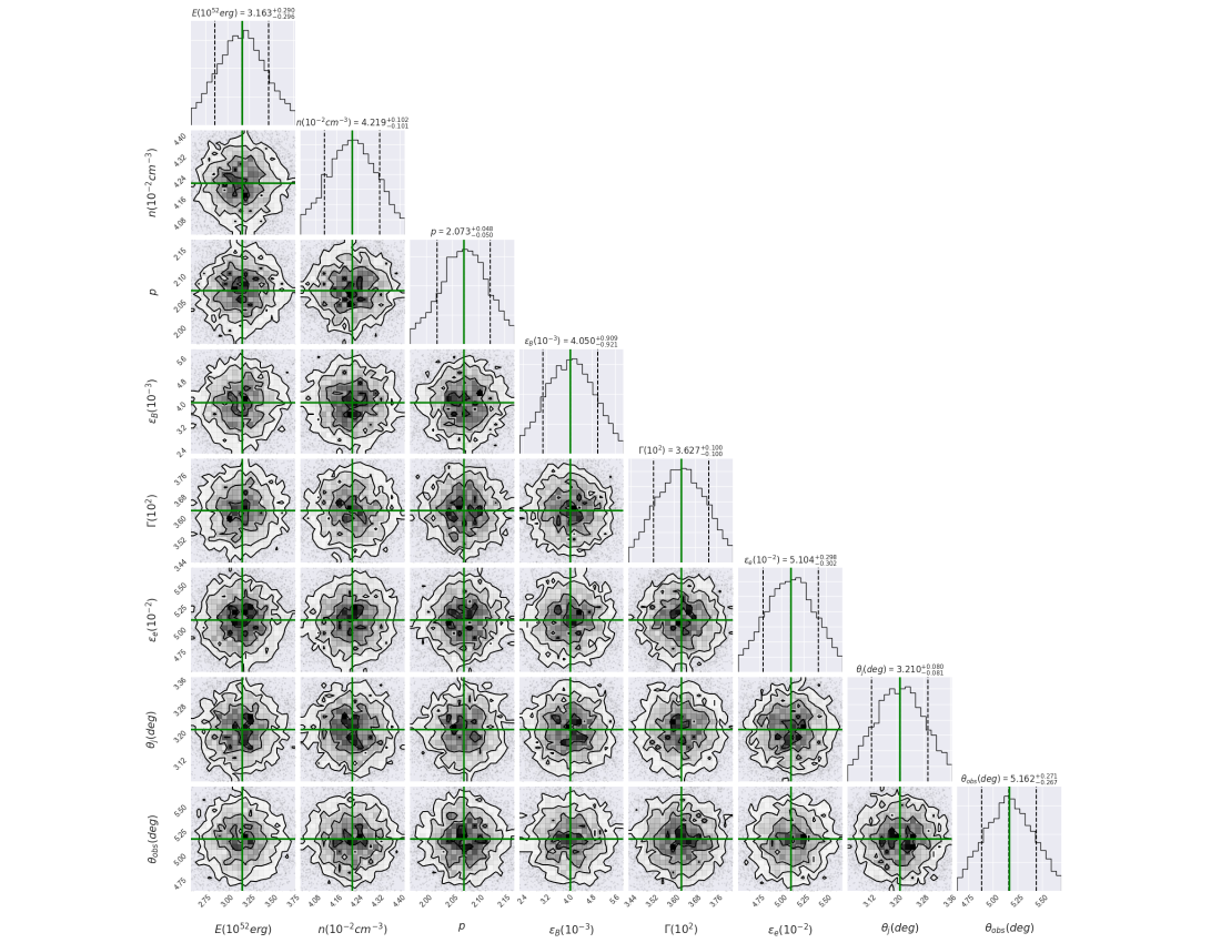
We apply the Bayesian statistical approach of Markov-Chain Monte Carlo (MCMC) simulations to determine the best-fit values of the parameters that characterize the multi-wavelength afterglow observations with their upper limits (e.g., see Fraija et al., 2019c). A set of eight parameters, { $E$ , $n$ , $p$ , $\varepsilon_{B}$ , $\Gamma$ , $\varepsilon_{e}$ , $\theta_{\rm j}$ and $\theta_{\rm obs}$ }, is required by our synchrotron afterglow model evolving in a constant-density medium to describe the multi-wavelength observations. A total of 17300 samples and 4100 tuning steps is used to describe the entire dataset. Normal distributions are used to characterize all the parameters. Corner plots illustrate the best-fit values and the median of the posterior distributions of the parameters, as shown in Figure 5, respectively. In this figure, the best-fit values are highlighted in green, and the median of the posterior distributions are presented in Table 5.

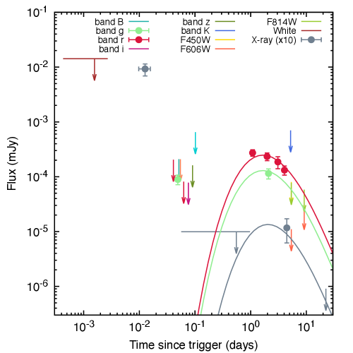
The multi-wavelength afterglow observations, together with the fits computed using the synchrotron off-axis model evolving in a constant-density medium are shown in Figure 4. The synchrotron light curves obtained with the same electron population and displayed in the optical (R and g) and X-ray bands support the scenario of one-emitting zone inside an off-axis outflow. The fact that the beaming cone of synchrotron radiation reaches our line of sight is compatible with the best-fit value of the viewing angle $\theta_{\rm obs}=15.412^{+0.268}_{-0.269}\,{\rm deg}$ and the re-brightening in all bands at $\sim$ one day. The best-fit value of the electron spectral index $p=2.319^{+0.049}_{-0.049}$ matches the typical value observed when forward-shocked electrons radiate by synchrotron emission (see, e.g. Kumar & Zhang, 2015). It confirms that these multi-wavelength observations originate during the afterglow.

The best-fit value of the constant-density medium $n=4.221^{+0.102}_{-0.103}\times 10^{-2}\,{\rm cm^{-3}}$ indicates that GRB 080503 took place in a medium with very low density comparable to an intergalactic density environment with $\sim 10^{-3}\,{\rm cm^{-3}}$ . The best-fit values of bulk Lorentz factor ( $\Gamma=2.939^{+0.101}_{-0.078}\times 10^{2}$ ) and the equivalent-kinetic energy ( $E=2.156^{+0.294}_{-0.295}\times 10^{52}\,{\rm erg}$ ) indicate that synchrotron radiation is emitted from a narrowly collimated outflow.

Perley et al. (2009) analyzed the multi-wavelength observations at $\sim$ one day. The authors dismissed the kilonova-like emission proposed by Li & Paczyński (1998) and gave an afterglow explanation, pointing out that the X-ray and optical data had similar evolutions. They hypothesized that the late optical and X-ray bumps might be explained in a slightly off-axis jet or a refreshed shock. The faint afterglow compared to the intense prompt emission could be described in the very low circumburst medium. Gao et al. (2015) claimed that under certain requirements on the bulk Lorentz factor and the beaming angle of the relativistic jet, refreshed shocks in the synchrotron forward- and reverse-shock scenario could adequately describe the late re-brightening in GRB 080503. Finally, Gao et al. (2015) proposed that the late optical peak was due to the emission from a magnetar-powered “merger-nova”, and the X-ray hump from magnetic dissipation of the magnetar dipole spin-down luminosity. According to our analysis, these observations at $\sim$ one day are consistent with the afterglow emission found off-axis. It is worth noting that measurements of the linear polarization of the optical emission could discriminate between an on- and off-axis scenario and gravitational waves would provide information about the progenitor (a merger of NS - NS, BH - NS or a stable NS.

GRB 140903A

We once again conducted MCMC simulations with a set of eight parameters, { $E$ , $n$ , $p$ , $\varepsilon_{B}$ , $\Gamma$ , $\varepsilon_{e}$ , $\theta_{\rm j}$ and $\theta_{\rm obs}$ }, to find the best-fit values that describe the multi-wavelength afterglow observations with their upper limits. A set of eight parameters, { $E$ , $n$ , $p$ , $\varepsilon_{B}$ , $\Gamma$ , $\varepsilon_{e}$ , $\theta_{\rm j}$ and $\theta_{\rm obs}$ }, is required. To represent the entire observations in this scenario, a total of 16200 samples and 4150 tuning steps were used. Figure 7 displays the best-fit values and the median of the posterior distributions of the parameters. In Table 5, the best-fit values are shown in green, and the median of the posterior distributions is presented.
The multi-wavelength observations of GRB 140903A are shown in Figure 6, together with the fits derived using the synchrotron off-axis model evolving in a homogenous density. The best-fit values of the viewing angle $\theta_{\rm obs}=5.162^{+0.271}_{-0.267}\,{\rm deg}$ and the half-opening angle $\theta_{\rm j}=3.210^{+0.080}_{-0.081}\,{\rm deg}$ indicate that the relativistic outflow was slightly off-axis. The best-fit value of the constant density medium $n=4.219^{+0.102}_{-0.101}\times 10^{-2}\,{\rm cm^{-3}}$ indicates that GRB 140903A took place in a medium with very low density comparable to an intergalactic density environment. The best-fit values of bulk Lorentz factor ( $\Gamma=3.627^{+0.100}_{-0.100}\times 10^{2}$ ) and the equivalent-kinetic energies ( $E=3.163^{+0.290}_{-0.296}\times 10^{52}\,{\rm erg}$ ) indicate that synchrotron emission is radiated from a narrowly collimated jet. The best-fit values of the microphysical parameters $\varepsilon_{\rm e}=5.104^{+0.298}_{-0.302}\times 10^{-2}$ and $\varepsilon_{\rm B}=4.050^{+0.909}_{-0.921}\times 10^{-3}$ , and the best-fit value of the spectral index of the shocked electrons $2.073^{+0.048}_{-0.050}$ , are similar to those reported in Troja et al. (2016). This spectral index is in the typical range to those accelerated in forward shocks (see, e.g. Kumar & Zhang, 2015), thus reaffirming the afterglow as its origin.

Troja et al. (2016) reported and analyzed the afterglow observations of GRB 140903A for the first two weeks. Applying the fireball scenario, the authors demonstrated that this burst was caused by a collimated jet seen off-axis and was also connected with a compact binary object. The X-ray ”plateau” seen in GRB 140903A was attributed to the energy injection into the decelerating blast wave by Zhang et al. (2017). The authors then modelled the late afterglow emission, which required a half-opening angle of $\approx 3\,{\rm deg}$ , similar to the value found with our model. GRB 140903A was formed in a collimated outflow observed off-axis that decelerates in a uniform density, according to our findings.

GRB 150101B

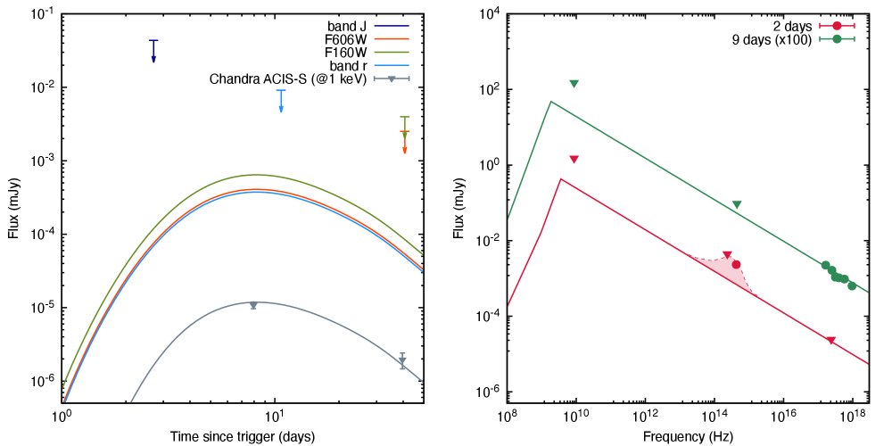
We use MCMC simulations with the eight parameters used for GRB 080503 and GRB 140903A to find the best-fit values that model the X-ray afterglow observations with the optical upper limits. To represent the entire data in this case, a total of 15900 samples and 4400 tuning steps are used. Figure 9 displays the best-fit values and the median of the posterior distributions of the parameters. In Table 5, the best-fit values are shown in green, and the median of the posterior distributions is presented.

The X-ray, optical and radio observations and upper limits, as well as the fit obtained using the synchrotron off-axis model evolving in homogeneous density are shown in Figure 8. The left-hand panel shows the light curves at 1 keV (gray), R-band (blue), F606W filter (orange) and F160W filter (dark green), and the right-hand panel displays the broadband SEDs at 2 (red) and 9 (green) days. The red area corresponds to the spectrum of AT2017gfo, which is adapted by Troja et al. (2018). The best-fit values of the viewing angle $\theta_{\rm obs}=14.114^{+2.327}_{-2.179}\,{\rm deg}$ and the half-opening angle $\theta_{\rm j}=6.887^{+0.662}_{-0.682}\,{\rm deg}$ can explain the lack of X-ray emission during the first day. The best-fit value of the constant density medium $n=0.164^{+0.021}_{-0.021}\times 10^{-2}\,{\rm cm^{-3}}$ indicates that GRB 150101B, like other short bursts, happened in an environment with very low density. The best-fit values of bulk Lorentz factor ( $\Gamma=4.251^{+0.468}_{-0.453}\times 10^{2}$ ) and the equivalent-kinetic energy ( $E=1.046^{+0.120}_{-0.124}\times 10^{52}\,{\rm erg}$ ) suggest that synchrotron afterglow emission is emitted from a narrowly collimated jet. The values of the spectral index of the electron population, the circumburst density, the microphysical parameters, and the viewing angle disfavor the isotropic cocoon model reported in Troja et al. (2018) and are consistent with the values of an outflow when homogeneous density is taken into account. The best-fit values of the spectral index of the shocked electrons $2.150^{+0.217}_{-0.215}$ is similar to those reported in synchrotron afterglow models (see, e.g. Kumar & Zhang, 2015).

GRB 160821B

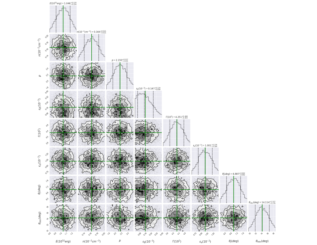
We require MCMC simulations with eight parameters used in the previous bursts to find the best-fit values that describe the multi-wavelength afterglow observations with their upper limits. To characterize the complete data in this scenario, a total of 17300 samples and 7400 tuning steps are used. Figure 11 exhibits the best-fit values and the median of the posterior distributions of the parameters. In Table 5, the best-fit values and the medians of the posterior distributions are presented.

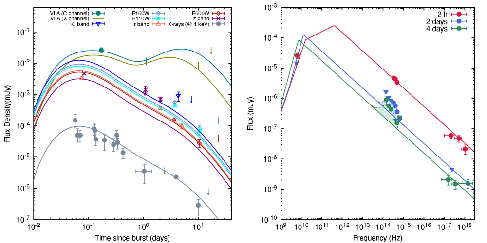
The multi-wavelength observations since 0.2 days after the GBM trigger are shown in Figure 10, together with the fits found requiring the synchrotron off-axis model evolving in a homogeneous density. The left-hand panel exhibits the light curves at 1 keV (gray), z-band (purple), F606W filter (dark red), R-band (salmon), F110W filter (cyan), F160W filter (blue sky), K_s-band (blue), X-channel (olive) and C-channel (emerald green), and the right-hand panel shows the broadband SEDs of the X-ray, optical and radio afterglow observations at 2 h (red), 2 days (blue) and 4 days (green). The shaded areas in blue and green correspond to blackbody spectra with decreasing temperatures firstly suggested in Jin et al. (2018) and then confirmed by Lamb et al. (2019) and Troja et al. (2019a). The kilonova emission is the most natural explanation for the “new” radiation component. The Swift-XRT-UVOT data were received from the public database from the official Swift website.³³3https://swift.gsfc.nasa.gov/cgi-bin/sdc/ql? The C-band displays radio data, the white, v, b, u, UVW1, UVW2, and UVM2 bands display Swift-UVOT data, and the 1 keV band displays XRT data. Using the conversion factor proposed in Evans et al. (2010), the flux density of XRT data is extrapolated from 10 keV to 1 keV. The best-fit values of circumburst density $n=0.869^{+0.093}_{-0.090}\times 10^{-2}\,{\rm cm^{-3}}$ , spectral index of shocked electrons $p=2.220^{+0.021}_{-0.021}$ , viewing angle $\theta_{\rm obs}=10.299^{+1.125}_{-1.135}\,{\rm deg}$ and the half-opening angle $\theta_{\rm j}=8.002^{+0.817}_{-0.809}\,{\rm deg}$ are similar to those previously reported in Troja et al. (2019b). The best-fit values of the viewing angle $\theta_{\rm obs}=10.299^{+1.125}_{-1.135}\,{\rm deg}$ and the half-opening angle $\theta_{\rm j}=8.002^{+0.817}_{-0.809}\,{\rm deg}$ suggest that the relativistic outflow was slightly off-axis. The best-fit values of bulk Lorentz factor ( $\Gamma=4.559^{+0.361}_{-0.358}\times 10^{2}$ ) and the equivalent-kinetic energy ( $E=0.118^{+0.021}_{-0.021}\times 10^{52}\,{\rm erg}$ ) indicate that synchrotron afterglow emission is emitted from a narrowly collimated jet.

SN 2020bvc

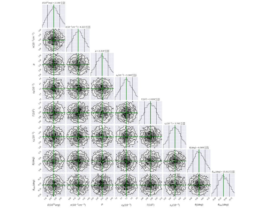
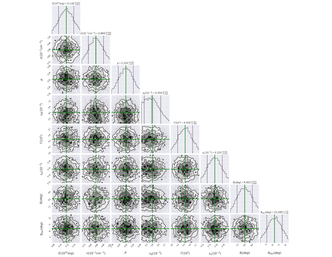
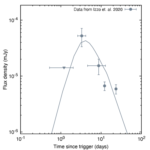
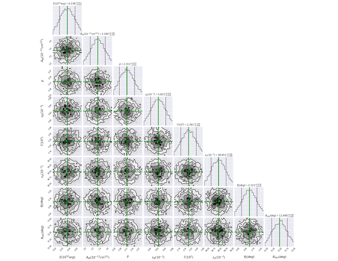
We use MCMC simulations to find the best-fit values of the parameters that describe the X-ray afterglow observations. A set of eight parameters, { $E$ , $A_{w}$ , $p$ , $\varepsilon_{B}$ , $\Gamma$ , $\varepsilon_{e}$ , $\theta_{\rm j}$ and $\theta_{\rm obs}$ }, is used to describe the X-ray observations. To characterize the complete data in this scenario, a total of 17100 samples and 7200 tuning steps are used. Figure 13 exhibits the best-fit values and the median of the posterior distributions of the parameters. In Table 5, the best-fit values are shown in green, and the medians of the posterior distributions are presented. We assumed a stratified medium with a parameter $k=1.5$ , consistent with the proposal by Izzo et al. (2020). Our best fit values, however, are slightly different. We propose that the emission is due to an off-axis jet that is $\approx 5$ times more energetic and with half of the off-axis angle compared to the values of Izzo et al. (2020). This discrepancy is due to a different choice of the electron velocity distribution index $p$ , as our MCMC simulation suggested $p=2.313^{+0.037}_{-0.035}$ , in contrast with the value of $p=2$ used by the cited authors. Figure 12 shows the X-ray observations of SN 2020bvc with the best-fit synchrotron light curve generated by the deceleration of an off-axis jet in a medium with stratification parameter $k=1.5$ .

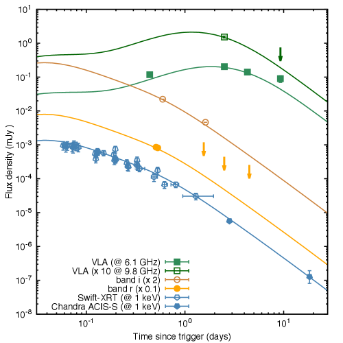
Our results are consistent with the X-ray observations before and after $\sim 4\,{\rm days}$ since the trigger time; when the observed flux increases and decreases, respectively. Initially, the flux increases with a minimum rise index of $\alpha_{\rm m,ris}>1.65$ and later the observed flux decreases with $\alpha_{\rm dec}=-1.35\pm 0.09$ (Izzo et al., 2020). The allowed value of the minimum rise index is estimated considering a simple power-law function, the X-ray upper limit and the maximum flux. For instance, given the best-fit value of $p=2.313^{+0.037}_{-0.035}$ and for $0<k<1.5$ , the temporal rise and decay indexes are $1.65\pm 0.03\leq\alpha_{\rm ris}\leq 4.53\pm 0.03$ and $\alpha_{\rm dec}=-1.24\pm 0.03$ , respectively, for $\nu_{\rm c}<\nu$ (see Table 1). For ${\rm k>1.5}$ , the expected rise index would be $\alpha_{\rm ris}<1.65$ , which cannot reproduce the X-ray observations.

The synchrotron scenario from on-axis outflow in a very-low density environment is disfavored for $p\sim 2$ . The closure relations of synchrotron on-axis model from an outflow decelerating in a stratified environment for $k$ in general can be estimated. During the coasting and the deceleration phases the bulk Lorentz factor evolves as $\Gamma\propto t^{0}$ and $\Gamma\propto t^{\frac{k-3}{8-2k}}$ , respectively. Therefore, the synchrotron flux during the slow-cooling regime evolves as $F_{\rm\nu}\propto t^{\frac{12-k(p+5)}{4}}\,\nu^{-\frac{p-1}{2}}$ for $\nu_{\rm m}<\nu<\nu_{\rm c}$ and $\propto t^{\frac{8-k(p+2)}{4}}\,\nu^{-\frac{p}{2}}$ for $\nu_{\rm c}<\nu$ during the coasting phase, and $F_{\rm\nu}\propto t^{-\frac{12(p-1)+k(5-3p)}{4(4-k)}}\nu^{-\frac{p-1}{2}}$ for $\nu_{\rm m}<\nu<\nu_{\rm c}$ and $\propto t^{-\frac{3p-2}{4}}\nu^{-\frac{p}{2}}$ for $\nu_{\rm c}<\nu$ , during the deceleration phase. It is worth noting that for the cooling condition $\nu_{\rm c}<\nu$ and with a value of $p=2.5$ , the temporal evolution is only consistent for $k\lesssim 0.3$

The best-fit values of bulk Lorentz factor ( $\Gamma=2.291^{+0.100}_{-0.100}\times 10^{2}$ ), the equivalent-kinetic energy ( $E=2.38^{+0.01}_{-0.01}\times 10^{51}\,{\rm erg}$ ) and the half-opening angle $\theta_{\rm j}=2.121^{+0.078}_{-0.079}\,{\rm deg}$ indicate that synchrotron emission is produced from a narrowly collimated outflow decelerating in an external medium. The best-fit values of the viewing angle $\theta_{\rm obs}=12.498^{+0.268}_{-0.281}\,{\rm deg}$ and the half-opening angle $\theta_{\rm j}=2.121^{+0.078}_{-0.079}\,{\rm deg}$ are consistent with the lack of early multi-wavelength observations.

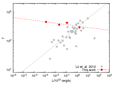
Lü et al. (2012) discovered a correlation between the bulk Lorentz factors and the isotropic gamma-ray luminosities in a sample of GRBs. Fan et al. (2012) showed that the correlation of these parameters were consistent with the parameters predicted in the photospheric emission model. Figure 14 shows the diagram of the bulk Lorentz factors and the isotropic gamma-ray luminosities of sGRBs described in this work (red) with those (gray) reported in Lü et al. (2012). For off-axis sGRBs, we found an empirical correlation $\Gamma=a({\rm L/10^{52}\,erg})^{b}$ with a = $(3.27\pm 0.39)\times 10^{2}$ and b = $-(4.9\pm 2.0)\times 10^{-2}$ .

4. Constrains on possible afterglow emission

4.1. The closest sGRBs detected by Swift ( $100\leq d_{z}\leq 200$ Mpc)

GRB 050906

Swift-BAT was triggered by GRB 050906 at 10:32:18 UTC on September 5, 2005, with a reported location of R.A.= $03^{\textrm{h}}31^{\textrm{m}}13^{\textrm{s}}$ and Dec= $-14^{\circ}37^{\prime}30^{\prime\prime}$ (J2000) with a positional accuracy of $3^{\prime}$ (Krimm et al., 2005). The light curve revealed an excess in the ( $25-100$ ) keV energy range. The duration and measured fluence in the energy range of 15 - 150 keV were $128\pm 16\ \textrm{ms}$ and $(5.9\pm 3.2)\times 10^{-8}\ \textrm{erg}\ \textrm{cm}^{-2}$ , respectively (Parsons et al., 2005). Levan et al. (2008) provided the specifics of Swift’s deep optical and infrared observations. According to the authors, no X-ray nor optical/IR afterglow was detected to deep limits, and no residual optical or IR emission was observed.

GRB 070810B

Swift-BAT was triggered by GRB 070810B at 15:19:17 UTC on August 10, 2007, with a reported location of $\textrm{R.A.}=00^{\textrm{h}}35^{\textrm{m}}46^{\textrm{s}}$ and $\textrm{Dec}=+08^{\circ}50^{\prime}07^{\prime\prime}$ (J2000) with a positional accuracy of $3^{\prime}$ (Marshall et al., 2007). The KANATA 1.5-m telescope, the Xinlong TNT 80 cm telescope, the 2-m Faulkes Telescope South, the Shajn 2.6 m telescope, and the Keck I telescope (HST) conducted follow-up observations after the initial detection, which are summarized in Bartos et al. (2019). From the whole observational campaign, only the Shajn telescope detected a source inside the error box of GRB 070810B (Rumyantsev et al., 2007).

GRB 080121

Swift-BAT was triggered by GRB 080121 at 21:29:55 UTC on January 21, 2008, with a reported location of $\textrm{R.A.}=09^{\textrm{h}}08^{\textrm{m}}56^{\textrm{s}}$ , $\textrm{Dec}=+41^{\circ}50^{\prime}29^{\prime\prime}$ (J2000) and a positional accuracy of $3^{\prime}$ . In the ( $15-150$ ) keV energy range, the duration and measured fluence were $(0.7\pm 0.2)\,\textrm{s}$ and $(3\pm 2)\times 10^{-8}\ \textrm{erg}\ \textrm{cm}^{-2}\ \textrm{s}^{-1}$ , respectively, according to Cummings & Palmer (2008). Follow-up observations were carried out 2.3 days following the burst using the Swift/UVOT and the Swift/XRT. Within the Swift-BAT error circle, however, no X-ray afterglow candidate or sources were discovered (Cucchiara & Schady, 2008; Troja & Burrows, 2008). Within the Swift-BAT error circle, two galaxies were found, indicating a redshift of $z\sim 0.046$ for GRB 080121, however the isotropic energy released would be several orders of magnitude lower than usual short-hard bursts (Perley et al., 2008d).

GRB 100216A

Swift-BAT and Fermi-GBM were triggered by GRB 100216A at 10:07:00 UTC on February 16, 2010 with a reported location of $\textrm{R.A.}=10^{\textrm{h}}17^{\textrm{m}}03.2^{\textrm{s}}$ , $\textrm{Dec}=+35^{\circ}31^{\prime}27.5^{\prime\prime}$ (J2000) with a positional accuracy of $3^{\prime}$ . In the energy range of ( $15-350$ ) keV, the duration and measured fluence of the single peak were $0.3\ \textrm{s}$ and $(4.7\pm 3)\times 10^{-8}\ \textrm{erg}\ \textrm{cm}^{-2}$ , respectively (Cummings et al., 2010). The burst was followed up by Swift-XRT and Swift-UVOT from $214.4$ to $249.2\ \textrm{ks}$ after the BAT trigger. Within the observation, no fading sources were found, but a source presumed to be 1RXS J101702.9+353404 was discovered within the error circle (Rowlinson et al., 2010; Siegel & Rowlinson, 2010).

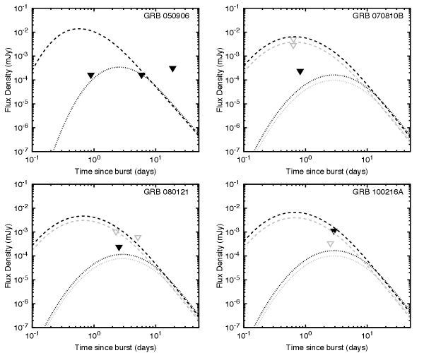
Figure 15 shows the UV and optical upper limits of the closest sGRBs detected by Swift between 100 and 200 Mpc with the synchrotron light curves from an off-axis outflow decelerating in a constant-density medium. The synchrotron light curves are exhibited at the R-band (black) and the UVW1-band (gray). The parameter values used to generate the synchrotron light curves are reported in Table Modeling Gamma-ray burst Afterglow observations with an Off-axis Jet emission. We report two values for each parameter; the upper values correspond to synchrotron light curves on the left-hand panels and lower ones on the right panels. For typical values of GRB afterglow reported in Table Modeling Gamma-ray burst Afterglow observations with an Off-axis Jet emission, the synchrotron emission is ruled out for a density of $n=1\,{\rm cm^{-3}}$ , but not for $n=10^{-2}\,{\rm cm^{-3}}$ . The value of the uniform-density medium ruled out in our model is consistent with the mean value reported for sGRBs (e.g., see Berger, 2014). It is worth noting that for values of $\varepsilon_{B}<10^{-4.3}$ and $\varepsilon_{e}<10^{-1.2}$ , the value of the density $n=1\,{\rm cm}^{-3}$ would be allowed.

4.2. Promising GW events in the third observing run (O3) that could generate electromagnetic emission

The Advanced LIGO and Advanced Virgo produced 56 non-retracted alerts of gravitational waves candidates during the O3 run, covering almost one year of operations (from 2019 April 01 to 2020 March 27). Nevertheless, three of them have a probability of being terrestrial larger than 50%. The O3 observing run was divided into two epochs associated to “O3a” (from April 01 to September 30) and “O3b” (from November 01 to March 27, 2020). The GW events in the O3a and O3b runs are listed in the Gravitational Wave Transient (GWTC-2) Catalog 2 (Abbott et al., 2021) and (GWTC-3) Catalog 3 (The LIGO Scientific Collaboration et al., 2021), respectively, where from GCNs there were 31 and 22 candidate events discovered during O3a and O3b respectively. The promising candidates that are consistent with a source with $m_{2}<3M_{\odot}$ and that could generate electromagnetic emission are GW190425, GW190426_152155, GW190814 in GWTC-2 (Abbott et al., 2021) and GW191219_163120, GW200105_162426, GW200115_042309, GW200210_092254 in GWTC-3 (The LIGO Scientific Collaboration et al., 2021). Table Modeling Gamma-ray burst Afterglow observations with an Off-axis Jet emission enumerates the main characteristics of these candidates.

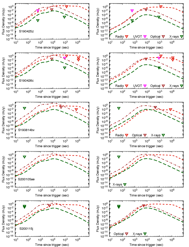
Figure 16 shows the multi-wavelength upper limits of GW events in GWTC-2 and GWTC-3 consistent with a source with $m_{2}<3M_{\odot}$ and that could generate electromagnetic emission and the synchrotron light curves from an off-axis outflow decelerating in a constant-density medium with $n=1\,{\rm cm^{-3}}$ (left panels) and $10^{-2}\,{\rm cm^{-3}}$ (right panels). The synchrotron light curves are presented at 1 keV (green), R-band (brown) (from Becerra et al. (2021a)) and 3 GHz (red). The parameter values used are $E=5\times 10^{50}\,{\rm erg}$ , $\theta_{\rm j}=3\,{\rm deg}$ , $\theta_{\rm obs}=6\,{\rm deg}$ , $\Gamma=100$ , $\varepsilon_{\rm e}=0.1$ , $p=2.5$ , $\zeta_{e}=1.0$ and $\varepsilon_{\rm B}=10^{-2}$ . The left-hand panels associated to the S190425z, S190426c, S190814bv and S200115j events show that a uniform-density is ruled out for $n=1\,{\rm cm^{-3}}$ , but not for $n=10^{-2}\,{\rm cm^{-3}}$ . For instance, we can note that in the panel related to S190426c the synchrotron emission at 1 keV, at the R-band and at 3 GHz is above the upper limits around $\sim$ one day for $n=1\,{\rm cm^{-3}}$ , and in the panel associated to S190814bv the synchrotron flux at the R-band and 3 GHz is above the upper limits, but not at 1 keV. The value of the constant-density medium ruled out in our model is consistent with the densities derived by Dobie et al. (2019); Ackley et al. (2020); Gomez et al. (2019) using distinct off-axis jet models. We need further observations on different timescales and energy bands to derive tighter constraints.

5. Conclusions

We have extended the synchrotron off-axis model presented in Fraija et al. (2019b) initially proposed to describe the multi-wavelength afterglow observations in GRB 170817A. In the current model, we have considered i) the circumburst external medium as stratified with a profile density $\propto r^{-k}$ with ${\rm k}$ in the range of $0\leq k\leq 3$ , ii) the synchrotron radiation in self-absorption regime, iii) the afterglow emission during the transition from off-axis to on-axis before the lateral expansion phase (relativistic phase), iv) the hydrodynamical evolution computed by numerical simulations and v) a fraction of electrons accelerated by the shock front. The time evolution of the Doppler factor, the half-opening angle, the bulk Lorentz factor, and the deceleration radius computed by numerical simulations are in good agreement with those derived with an analytical approach. The advantage of this general approach (with a density profile $A_{\rm k}\propto r^{-k}$ ) is that this model allows us to take into account not only both a homogeneous medium ( $k=0$ ) and a wind-like medium ( $k=2$ ) but regions with non-standard stratification parameters, such as $k=1.0$ , $1.5$ or $2.5$ .

We have calculated the synchrotron light curves and presented the closure relations in a stratified environment, including the self-absorption regime for all cooling conditions during the coasting, deceleration (off- and on-axis emission), and the post-jet-break decay phases. We have noted that a break is expected around the transition between fast- and slow-cooling regimes during the deceleration phase when the afterglow emission seems off-axis, but not during other stages. We have analyzed the behavior of the flux for different parameters of the density distribution. We have noticed that the behavior during the relativistic phase approaches flatness as the stratification parameter is raised. On the other hand, we have shown that the time evolution of the light curves after the jet break is independent of $k$ , so this model gives freedom to explain the early-time evolution of the radiation while keeping the long-time results invariant. Furthermore, we have derived the change of the density parameter in the entire phase. We have shown that: In general, during the coasting and the deceleration phases, when the afterglow emission seems off-axis, a transition between different environments cannot be detected, contrary to the post-jet-break phase and the deceleration phase with on-axis emission. The synchrotron fluxes do not depend on the density parameter when these are observed at the lowest and the highest frequencies when the afterglow emission seems off- and on-axis, respectively. During the post-jet-break phase, any transition between a stratified environment and density-constant medium will be better observed in low frequencies, such as radio wavelengths.

In particular, we have applied our model to describe the delayed non-thermal emission observed in a sample of bursts with evidence of off-axis emission. In accordance with the best-fit values for sGRBs, we found that i) the constant-density medium required to model the multi-wavelength observations is low ( $10^{-2}\leq n\leq 0.4\,{\rm cm^{-3}}$ ), indicating that the central engine are located in a low density circumstellar medium, ii) the spectral indexes of the shocked electrons ( $2.1\leq p\leq 2.3$ ) are in the range of those reported after the description of the afterglow observations (see, e.g. Kumar & Zhang, 2015; Fraija et al., 2017; Becerra et al., 2019a, b, c, 2021b), and iii) the half-opening angles ( $1.5\leq\theta_{\rm j}\leq 6.6\,{\rm deg}$ ), the bulk Lorentz factors ( $130\leq\Gamma\leq 450$ ) and the equivalent-kinetic energies ( $0.2\leq E\leq 5.7\times 10^{52}\,{\rm erg}$ ) provide evidence of narrowly collimated outflow expanding into a constant-density environment. The previous results confirm that the multi-wavelength observations are emitted from the GRB afterglow and indicate a merger of compact objects (two NSs or NS-BH) as possible progenitors of these bursts. The low-density medium agrees with the larger offsets of sGRBs compared with lGRBs. Regarding SN 2020bvc, we found that an atypical stratification parameter of $k=1.5$ is required, supporting the CC-SN scenario. The best-fit values of the half-opening angle $2.121^{+0.078}_{-0.079}\,{\rm deg}$ , the viewing angle $12.498^{+0.268}_{-0.281}\,{\rm deg}$ , the equivalent-kinetic energy $2.38^{+0.11}_{-0.10}\times 10^{51}\,{\rm erg}$ and the bulk-Lorentz factor $2.291^{+0.100}_{-0.100}\times 10^{2}$ provide evidence of the scenario of off-axis GRB afterglow.

We have applied the current model to provide constraints on the possible afterglow emission using multi-wavelength upper limits associated with the closest Swift-detected sGRBs ( $<200\ \mathrm{Mpc}$ ) and the promising GW events. We have shown that the value of the constant-density medium is ruled out, which is consistent with the mean value of densities reported in for sGRBs (e.g., see Berger, 2014) and those derived by S190814bv event (e.g., see Dobie et al., 2019; Ackley et al., 2020; Gomez et al., 2019) using different models. To derive tighter constraints, further observations on timescales from months to years post-merger phase are required.

ACKNOWLEDGEMENTS

We would like to express our gratitude to the anonymous referee for his or her careful reading of the manuscript and insightful recommendations that helped improve the paper’s quality and clarity. We thank Rodolfo Barniol Duran, Tanmoy Laskar, Paz Beniamini and Bing Zhang for useful discussions. NF acknowledges financial support from UNAM-DGAPA-PAPIIT through grant IN106521. RLB acknowledges support from CONACyT postdoctoral fellowships and the support from the DGAPA/UNAM IG100820 and IN105921.

References

Abbott et al. (2017a) Abbott, B. P., Abbott, R., Abbott, T. D., & et al. 2017a, Phys. Rev. Lett., 119, 161101
Abbott et al. (2017b) —. 2017b, The Astrophysical Journal Letters, 848, L12
Abbott et al. (2017) Abbott, B. P., Abbott, R., Abbott, T. D., et al. 2017, ApJ, 848, L13
Abbott et al. (2021) Abbott, R., Abbott, T. D., Abraham, S., et al. 2021, Physical Review X, 11, 021053
Ackley et al. (2020) Ackley, K., Amati, L., Barbieri, C., et al. 2020, arXiv e-prints, arXiv:2002.01950
Alexander et al. (2017) Alexander, K. D., Berger, E., Fong, W., et al. 2017, ApJ, 848, L21
Alexander et al. (2018) Alexander, K. D., Margutti, R., Blanchard, P. K., et al. 2018, ArXiv e-prints, arXiv:1805.02870
Andreoni et al. (2020) Andreoni, I., Goldstein, D. A., Kasliwal, M. M., et al. 2020, ApJ, 890, 131
Barthelmy et al. (2005) Barthelmy, S. D., Cannizzo, J. K., Gehrels, N., et al. 2005, ApJ, 635, L133
Bartos et al. (2019) Bartos, I., Lee, K. H., Corsi, A., Márka, Z., & Márka, S. 2019, MNRAS, 485, 4150
Becerra et al. (2019a) Becerra, R. L., De Colle, F., Watson, A. M., et al. 2019a, ApJ, 887, 254
Becerra et al. (2019b) Becerra, R. L., Watson, A. M., Fraija, N., et al. 2019b, ApJ, 872, 118
Becerra et al. (2019c) Becerra, R. L., Dichiara, S., Watson, A. M., et al. 2019c, ApJ, 881, 12
Becerra et al. (2021a) —. 2021a, MNRAS, 507, 1401
Becerra et al. (2021b) Becerra, R. L., De Colle, F., Cantó, J., et al. 2021b, ApJ, 908, 39
Berger (2014) Berger, E. 2014, ARA&A, 52, 43
Blandford & McKee (1976) Blandford, R. D., & McKee, C. F. 1976, Physics of Fluids, 19, 1130
Blondin et al. (1996) Blondin, J. M., Lundqvist, P., & Chevalier, R. A. 1996, ApJ, 472, 257
Bloom & Perley (2008) Bloom, J. S., & Perley, D. A. 2008, GRB Coordinates Network, 7667
Bloom et al. (1999) Bloom, J. S., Kulkarni, S. R., Djorgovski, S. G., et al. 1999, Nature, 401, 453
Bloom et al. (2008) Bloom, J. S., Li, W., Levan, A. J., et al. 2008, GRB Coordinates Network, 7703
Bochenek (2019a) Bochenek, C. 2019a, LIGO/Virgo S190425z: STARE2 simultaneous L-band radio observations, The Gamma-ray Coordinates Network
Bochenek (2019b) —. 2019b, LIGO/Virgo S190426c: STARE2 simultaneous L-band radio observations, The Gamma-ray Coordinates Network
Brown & Mao (2008) Brown, P. J., & Mao, J. 2008, GRB Coordinates Network, 7675
Burns et al. (2018) Burns, E., Veres, P., Connaughton, V., et al. 2018, ApJ, 863, L34
Cenko et al. (2014) Cenko, S. B., Capone, J., Toy, V., et al. 2014, GRB Coordinates Network, Circular Service, No. 16785, #1 (2014), 16785
Chevalier (1982) Chevalier, R. A. 1982, ApJ, 258, 790
Chevalier (1984) —. 1984, ApJ, 285, L63
Corsi (2019) Corsi, A. 2019, LIGO/Virgo S190426c: VLA Follow-Up Observations of ZTF19aassfws, The Gamma-ray Coordinates Network
Coulter et al. (2017) Coulter, D. A., Foley, R. J., Kilpatrick, C. D., et al. 2017, Science, 358, 1556
Cucchiara et al. (2014) Cucchiara, A., Cenko, S. B., Perley, D. A., Capone, J., & Toy, V. 2014, GRB Coordinates Network, Circular Service, No. 16774, #1 (2014), 16774
Cucchiara & Schady (2008) Cucchiara, A., & Schady, P. 2008, GRB Coordinates Network, 7217
Cummings (2014) Cummings, J. R. 2014, GRB Coordinates Network, Circular Service, No. 16765, #1 (2014), 16765
Cummings (2015) —. 2015, GRB Coordinates Network, Circular Service, No. 17267, #1 (2015), 17267
Cummings et al. (2010) Cummings, J. R., Barthelmy, S. D., Fox, D. B., et al. 2010, GRB Coordinates Network, 10428
Cummings et al. (2014) Cummings, J. R., Burrows, D. N., Evans, P. A., et al. 2014, GRB Coordinates Network, Circular Service, No. 16763, #1 (2014), 16763
Cummings & Palmer (2008) Cummings, J. R., & Palmer, M. 2008, GRB Coordinates Network, 7209
D’Avanzo et al. (2015) D’Avanzo, P., D’Elia, V., Lorenzi, V., et al. 2015, GRB Coordinates Network, Circular Service, No. 17326, #1 (2015), 17326
D’Avanzo et al. (2018) D’Avanzo, P., Campana, S., Salafia, O. S., et al. 2018, ArXiv e-prints, arXiv:1801.06164
Dichiara et al. (2014) Dichiara, S., Guidorzi, C., & Japelj, J. 2014, GRB Coordinates Network, Circular Service, No. 16781, #1 (2014), 16781
Dichiara et al. (2020) Dichiara, S., Troja, E., O’Connor, B., et al. 2020, MNRAS, 492, 5011
Dobie et al. (2019) Dobie, D., Stewart, A., Murphy, T., et al. 2019, ApJ, 887, L13
Dobie et al. (2018) Dobie, D., Kaplan, D. L., Murphy, T., et al. 2018, ApJ, 858, L15
Duncan & Thompson (1992) Duncan, R. C., & Thompson, C. 1992, ApJ, 392, L9
Evans et al. (2016) Evans, P. A., Goad, M. R., Osborne, J. P., & Beardmore, A. P. 2016, GRB Coordinates Network, 19837, 1
Evans et al. (2010) Evans, P. A., Willingale, R., Osborne, J. P., et al. 2010, A&A, 519, A102
Fan & Piran (2006) Fan, Y., & Piran, T. 2006, MNRAS, 369, 197
Fan et al. (2012) Fan, Y.-Z., Wei, D.-M., Zhang, F.-W., & Zhang, B.-B. 2012, The Astrophysical Journal, 755, L6
Fong (2014) Fong, W. 2014, GRB Coordinates Network, Circular Service, No. 16777, #1 (2014), 16777
Fong (2015) —. 2015, GRB Coordinates Network, Circular Service, No. 17288, #1 (2015), 17288
Fong et al. (2015) Fong, W., Berger, E., Fox, D., & Shappee, B. J. 2015, GRB Coordinates Network, Circular Service, No. 17333, #1 (2015), 17333
Fong et al. (2016) Fong, W., Margutti, R., Chornock, R., et al. 2016, ApJ, 833, 151
Fraija (2015) Fraija, N. 2015, ApJ, 804, 105
Fraija et al. (2019a) Fraija, N., De Colle, F., Veres, P., et al. 2019a, ApJ, 871, 123
Fraija et al. (2017) Fraija, N., Lee, W. H., Araya, M., et al. 2017, ApJ, 848, 94
Fraija et al. (2019b) Fraija, N., Lopez-Camara, D., Pedreira, A. C. C. d. E. S., et al. 2019b, ApJ, 884, 71
Fraija et al. (2019c) Fraija, N., Pedreira, A. C. C. d. E. S., & Veres, P. 2019c, ApJ, 871, 200
Frail & Chandra (2008) Frail, D. A., & Chandra, P. 2008, GRB Coordinates Network, 7684
Galama et al. (1998) Galama, T. J., Vreeswijk, P. M., van Paradijs, J., et al. 1998, Nature, 395, 670
Gao et al. (2015) Gao, H., Ding, X., Wu, X.-F., Dai, Z.-G., & Zhang, B. 2015, ApJ, 807, 163
Giblin et al. (1999) Giblin, T. W., van Paradijs, J., Kouveliotou, C., et al. 1999, ApJ, 524, L47
Gomez et al. (2019) Gomez, S., Hosseinzadeh, G., Cowperthwaite, P. S., et al. 2019, ApJ, 884, L55
Granot et al. (2017) Granot, J., Gill, R., Guetta, D., & De Colle, F. 2017, ArXiv e-prints, arXiv:1710.06421
Granot et al. (2002) Granot, J., Panaitescu, A., Kumar, P., & Woosley, S. E. 2002, ApJ, 570, L61
Guidorzi & Mao (2008) Guidorzi, C., & Mao, J. 2008, GRB Coordinates Network, 7674
Haggard et al. (2018) Haggard, D., Nynka, M., Ruan, J. J., Evans, P., & Kalogera, V. 2018, The Astronomer’s Telegram, 11242
Hiramatsu et al. (2020) Hiramatsu, D., Arcavi, I., Burke, J., et al. 2020, Transient Name Server Classification Report, No. 2020-403, 1
Ho (2020) Ho, A. Y. Q. 2020, Transient Name Server AstroNote 2020-42, 1
Ho et al. (2020a) Ho, A. Y. Q., Cenko, B., Perley, D., Corsi, A., & Brightman, M. 2020a, Transient Name Server AstroNote 2020-45, 1
Ho et al. (2020b) Ho, A. Y. Q., Kulkarni, S. R., Perley, D. A., et al. 2020b, ApJ, 902, 86
Hotokezaka et al. (2018) Hotokezaka, K., Kiuchi, K., Shibata, M., Nakar, E., & Piran, T. 2018, ApJ, 867, 95
Huang et al. (1999) Huang, Y. F., Dai, Z. G., & Lu, T. 1999, MNRAS, 309, 513
Huang et al. (2000) —. 2000, MNRAS, 316, 943
Ioka & Nakamura (2017) Ioka, K., & Nakamura, T. 2017, ArXiv e-prints, arXiv:1710.05905
Izzo et al. (2020) Izzo, L., Auchettl, K., Hjorth, J., et al. 2020, A&A, 639, L11
Jin et al. (2018) Jin, Z.-P., Li, X., Wang, H., et al. 2018, ApJ, 857, 128
Kasliwal et al. (2017) Kasliwal, M. M., Nakar, E., Singer, L. P., et al. 2017, Science, 358, 1559
Kotak et al. (2004) Kotak, R., Meikle, W. P. S., Adamson, A., & Leggett, S. K. 2004, MNRAS, 354, L13
Kouveliotou et al. (1993) Kouveliotou, C., Meegan, C. A., Fishman, G. J., et al. 1993, The Astrophysical Journal, 413, L101
Krimm et al. (2005) Krimm, H., La Parola, V., de Pasquale, M., et al. 2005, GRB Coordinates Network, 3926, 1
Kumar et al. (2008) Kumar, P., Narayan, R., & Johnson, J. L. 2008, Science, 321, 376
Kumar & Zhang (2015) Kumar, P., & Zhang, B. 2015, Phys. Rep., 561, 1
Lamb et al. (2019) Lamb, G. P., Tanvir, N. R., Levan, A. J., et al. 2019, ApJ, 883, 48
Lazzati et al. (2017) Lazzati, D., Perna, R., Morsony, B. J., et al. 2017, ArXiv e-prints, arXiv:1712.03237
Levan et al. (2015) Levan, A. J., Hjorth, J., Wiersema, K., & Tanvir, N. R. 2015, GRB Coordinates Network, Circular Service, No. 17281, #1 (2015), 17281
Levan et al. (2016) Levan, A. J., Wiersema, K., Tanvir, N. R., et al. 2016, GRB Coordinates Network, 19846, 1
Levan et al. (2008) Levan, A. J., Tanvir, N. R., Jakobsson, P., et al. 2008, MNRAS, 384, 541
Li & Paczyński (1998) Li, L.-X., & Paczyński, B. 1998, ApJ, 507, L59
Lien (2020) Lien, A. 2020, LIGO/Virgo S200115j: no counterpart candidates in the Swift/BAT observations, The Gamma-ray Coordinates Network
Lien et al. (2016) Lien, A., Sakamoto, T., Barthelmy, S. D., et al. 2016, ApJ, 829, 7
LIGO Scientific Collaboration & Virgo Collaboration (2019) LIGO Scientific Collaboration, & Virgo Collaboration. 2019, GRB Coordinates Network, 25324, 1
Lü et al. (2017) Lü, H.-J., Zhang, H.-M., Zhong, S.-Q., et al. 2017, ApJ, 835, 181
Lü et al. (2012) Lü, J., Zou, Y.-C., Lei, W.-H., et al. 2012, The Astrophysical Journal, 751, 49
Lyman et al. (2018) Lyman, J. D., Lamb, G. P., Levan, A. J., et al. 2018, ArXiv e-prints, arXiv:1801.02669
Mao et al. (2008) Mao, J., Guidorzi, C., Ukwatta, T., et al. 2008, GCN Report, 138, 1
Margutti et al. (2017a) Margutti, R., Fong, W., Eftekhari, T., et al. 2017a, The Astronomer’s Telegram, 11037
Margutti et al. (2017b) Margutti, R., Berger, E., Fong, W., et al. 2017b, ApJ, 848, L20
Margutti et al. (2018) Margutti, R., Alexander, K. D., Xie, X., et al. 2018, ArXiv e-prints, arXiv:1801.03531
Marshall et al. (2007) Marshall, F. E., Brown, P. J., Cummings, J. R., et al. 2007, GRB Coordinates Network, 6743, 1
Metzger et al. (2011) Metzger, B. D., Giannios, D., Thompson, T. A., Bucciantini, N., & Quataert, E. 2011, MNRAS, 413, 2031
Mooley et al. (2017) Mooley, K. P., Nakar, E., Hotokezaka, K., et al. 2017, ArXiv e-prints, arXiv:1711.11573
Moriya & Tominaga (2012) Moriya, T. J., & Tominaga, N. 2012, ApJ, 747, 118
Nakar & Piran (2018) Nakar, E., & Piran, T. 2018, ArXiv e-prints, arXiv:1801.09712
Narayan et al. (1992) Narayan, R., Paczynski, B., & Piran, T. 1992, ApJ, 395, L83
Palmer et al. (2016) Palmer, D. M., Barthelmy, S. D., Cummings, J. R., et al. 2016, GRB Coordinates Network, 19844, 1
Panaitescu & Mészáros (1998) Panaitescu, A., & Mészáros, P. 1998, ApJ, 501, 772
Parsons et al. (2005) Parsons, A., Sarazin, C., Barbier, L., et al. 2005, GRB Coordinates Network, 3935, 1
Perley et al. (2020) Perley, D., Schulze, S., & Bruch, R. 2020, Transient Name Server AstroNote 2020-37, 1
Perley et al. (2008a) Perley, D. A., Bloom, J. S., & Li, W. 2008a, GRB Coordinates Network, 7695
Perley et al. (2008b) Perley, D. A., Bloom, J. S., & Prochaska, J. X. 2008b, GRB Coordinates Network, 7678
Perley et al. (2008c) —. 2008c, GRB Coordinates Network, 7679
Perley et al. (2008d) Perley, D. A., Foley, R. J., & Bloom, J. S. 2008d, GRB Coordinates Network, 7210
Perley et al. (2008e) Perley, D. A., Lai, D., Rockosi, C., & Bloom, J. S. 2008e, GRB Coordinates Network, 7666
Perley et al. (2008f) Perley, D. A., Bloom, J. S., Levan, A. J., et al. 2008f, GRB Coordinates Network, 7749
Perley et al. (2009) Perley, D. A., Metzger, B. D., Granot, J., et al. 2009, ApJ, 696, 1871
Planck Collaboration et al. (2016) Planck Collaboration, Ade, P. A. R., Aghanim, N., et al. 2016, A&A, 594, A13
Ramirez-Ruiz et al. (2005) Ramirez-Ruiz, E., Garcia-Segura, G., Salmonson, J. D., & Perez-Rendon, B. 2005, ApJ, 631, 435
Rhoads (1999) Rhoads, J. E. 1999, ApJ, 525, 737
Rhodes (2019) Rhodes, L. 2019, LIGO/Virgo S190426c: AMI-LA radio observations of ZTF19aassfws, The Gamma-ray Coordinates Network
Ridnaia (2020a) Ridnaia, A. 2020a, LIGO/Virgo S200105ae: Upper limits from Konus-Wind observations, The Gamma-ray Coordinates Network
Ridnaia (2020b) —. 2020b, LIGO/Virgo S200115j: Upper limits from Konus-Wind observations, The Gamma-ray Coordinates Network
Rowlinson et al. (2010) Rowlinson, A., Page, K., & Lyons, N. 2010, GRB Coordinates Network, 10435
Rumyantsev et al. (2007) Rumyantsev, V., Biryukov, V., & Pozanenko, A. 2007, GRB Coordinates Network, 6762, 1
Sakamoto et al. (2014) Sakamoto, T., Troja, E., Gehrels, N., et al. 2014, GRB Coordinates Network, Circular Service, No. 16813, #1 (2014), 16813
Sari & Esin (2001) Sari, R., & Esin, A. A. 2001, ApJ, 548, 787
Sari & Piran (1999) Sari, R., & Piran, T. 1999, A&AS, 138, 537
Sari et al. (1999) Sari, R., Piran, T., & Halpern, J. P. 1999, ApJ, 519, L17
Sari et al. (1998) Sari, R., Piran, T., & Narayan, R. 1998, ApJ, 497, L17
Savchenko et al. (2017) Savchenko, V., Ferrigno, C., Kuulkers, E., et al. 2017, ApJ, 848, L15
Siegel (2019) Siegel, M. 2019, LIGO/Virgo S190425z: Transient found in Swift/UVOT counterpart search, The Gamma-ray Coordinates Network
Siegel et al. (2016) Siegel, M. H., Barthelmy, S. D., Burrows, D. N., et al. 2016, GRB Coordinates Network, 19833, 1
Siegel & Rowlinson (2010) Siegel, M. H., & Rowlinson, A. 2010, GRB Coordinates Network, 10442
Soderberg et al. (2006) Soderberg, A. M., Chevalier, R. A., Kulkarni, S. R., & Frail, D. A. 2006, ApJ, 651, 1005
Stanbro (2015) Stanbro, M. 2015, GRB Coordinates Network, Circular Service, No. 17295, #1 (2015), 17295
Stanbro & Meegan (2016) Stanbro, M., & Meegan, C. 2016, GRB Coordinates Network, 19843, 1
Stanek (2020) Stanek, K. 2020, Transient Name Server Discovery Report, No. 2020-381, 1
The LIGO Scientific Collaboration et al. (2021) The LIGO Scientific Collaboration, the Virgo Collaboration, the KAGRA Collaboration, et al. 2021, arXiv e-prints, arXiv:2111.03606
Thompson (1994) Thompson, C. 1994, MNRAS, 270, 480
Tohuvavohu (2019a) Tohuvavohu, A. 2019a, LIGO/Virgo S190425z: Swift/UVOT and XRT pre-images at the position of the potential Swift/UVOT counterpart, The Gamma-ray Coordinates Network
Tohuvavohu (2019b) —. 2019b, LIGO/Virgo S190426c: Swift rapid follow-up observations of S190425z and S190426c and URL for observation log for all future events, The Gamma-ray Coordinates Network
Troja & Burrows (2008) Troja, E., & Burrows, D. N. 2008, GRB Coordinates Network, 7224
Troja et al. (2017) Troja, E., Lipunov, V. M., Mundell, C. G., & et al. 2017, Nature, 547, 425
Troja et al. (2017) Troja, E., Piro, L., van Eerten, H., & et al. 2017, Nature, 000, 1
Troja et al. (2016) Troja, E., Sakamoto, T., Cenko, S. B., et al. 2016, ApJ, 827, 102
Troja et al. (2018) Troja, E., Ryan, G., Piro, L., et al. 2018, Nature Communications, 9, 4089
Troja et al. (2019a) Troja, E., Castro-Tirado, A. J., Becerra González, J., et al. 2019a, MNRAS, 489, 2104
Troja et al. (2019b) Troja, E., Castro-Tirado, A. J., Gonzalez, J. B., et al. 2019b, arXiv e-prints, arXiv:1905.01290
Ukwatta et al. (2008) Ukwatta, T., Stamatikos, M., Sakamoto, T., Norris, J., & Barthelmy, S. D. 2008, GRB Coordinates Network, 7677
Usov (1992) Usov, V. V. 1992, Nature, 357, 472
van Marle et al. (2006) van Marle, A. J., Langer, N., Achterberg, A., & Garcia-Segura, G. 2006, A&AS, 460, 105
Vieira et al. (2020) Vieira, N., Ruan, J. J., Haggard, D., et al. 2020, arXiv e-prints, arXiv:2003.09437
von Kienlin et al. (2017) von Kienlin, A., Meegan, C., & Goldstein, A. 2017, GRB Coordinates Network, Circular Service, No. 21520, #1 (2017), 21520
Wang et al. (2010) Wang, X.-Y., He, H.-N., Li, Z., Wu, X.-F., & Dai, Z.-G. 2010, ApJ, 712, 1232
Watson et al. (2020) Watson, A. M., Butler, N. R., Lee, W. H., et al. 2020, MNRAS, 492, 5916
Waxman (1997) Waxman, E. 1997, ApJ, 491, L19
Weinberg (1972) Weinberg, S. 1972, Gravitation and Cosmology
Woosley (1993) Woosley, S. E. 1993, ApJ, 405, 273
Woosley & Bloom (2006) Woosley, S. E., & Bloom, J. S. 2006, ARA&A, 44, 507
Yamazaki et al. (2006) Yamazaki, R., Toma, K., Ioka, K., & Nakamura, T. 2006, MNRAS, 369, 311
Yi et al. (2013) Yi, S. X., Wu, X. F., & Dai, Z. G. 2013, ApJ, 776, 120
Zhang et al. (2017) Zhang, S., Jin, Z.-P., Wang, Y.-Z., & Wei, D.-M. 2017, ApJ, 835, 73

Table 1Evolution of the synchrotron light curves (

F_{\nu}\propto t^{-\alpha}\nu^{-\beta}

) from an off-axis outflow decelerated in a stratified environment

\cdashline1-6	$\beta$	$\alpha$	$\alpha$	$\alpha$	$\alpha$
		Coasting phase	Deceleration phase	Deceleration phase	Post jet-break phase
			(off-axis afterglow)	(on-axis afterglow)
$\nu_{\rm a,3}<\nu_{\rm c}<\nu_{\rm m}$
$\nu<\nu_{\rm a,3}$	$-2$	$-(1+k)$	$-4$	$-\frac{4}{4-k}$	$-1$
$\nu_{\rm a,3}<\nu<\nu_{\rm c}$	$-\frac{1}{3}$	$\frac{6k-11}{3}$	$\frac{8k-17}{3}$	$\frac{3k-2}{3(4-k)}$	$1$
$\nu_{\rm c}<\nu<\nu_{\rm m}$	$\frac{1}{2}$	$\frac{3k-8}{4}$	$\frac{9k-26}{4}$	$\frac{1}{4}$	$1$
$\nu_{\rm m}<\nu$	$\frac{p}{2}$	$\frac{k(p+2)-8}{4}$	$\frac{6(p-5)-(p-11)k}{4}$	$\frac{3p-2}{4}$	$p$
$\nu_{\rm a,1}<\nu_{\rm m}<\nu_{\rm c}$
$\nu<\nu_{\rm a,1}$	$-2$	$-2$	$-2$	$-\frac{2}{4-k}$	$0$
$\nu_{\rm a,1}<\nu<\nu_{\rm m}$	$-\frac{1}{3}$	$\frac{4k-9}{3}$	$\frac{8k-21}{3}$	$\frac{k-2}{4-k}$	$\frac{1}{3}$
$\nu_{\rm m}<\nu<\nu_{\rm c}$	$\frac{p-1}{2}$	$\frac{k(p+5)-12}{4}$	$\frac{6(p-5)-(p-11)k}{4}$	$-\frac{12(1-p)+k(3p-5)}{4(4-k)}$	$p$
$\nu_{\rm c}<\nu$	$\frac{p}{2}$	$\frac{k(p+2)-8}{4}$	$\frac{2(3p-16)-(p-10)k}{4}$	$\frac{3p-2}{4}$	$p$
$\nu_{\rm m}<\nu_{\rm a,2}<\nu_{\rm c}$
$\nu<\nu_{\rm m}$	$-2$	$-2$	$-2$	$-\frac{2}{4-k}$	$0$
$\nu_{\rm m}<\nu<\nu_{\rm a,2}$	$-\frac{5}{2}$	$-\frac{8+k}{4}$	$\frac{k-14}{4}$	$\frac{3k-20}{4(4-k)}$	$-1$
$\nu_{\rm a,2}<\nu<\nu_{\rm c}$	$\frac{p-1}{2}$	$\frac{k(p+5)-12}{4}$	$\frac{6(p-5)-(p-11)k}{4}$	$-\frac{12(1-p)+k(3p-5)}{4(4-k)}$	$p$
$\nu_{\rm c}<\nu$	$\frac{p}{2}$	$\frac{k(p+2)-8}{4}$	$\frac{2(3p-16)-(p-10)k}{4}$	$\frac{3p-2}{4}$	$p$

Table 2Closure relations of synchrotron radiation from off-axis afterglow model in a stratified environment

		Coasting phase	Deceleration phase	Deceleration phase	Post jet-break phase
			(off-axis afterglow)	(on-axis afterglow)
\cdashline1-6 $\nu_{\rm a,3}<\nu_{\rm c}<\nu_{\rm m}$
$\nu<\nu_{\rm a,3}$	$-2$	$\frac{(k+1)\beta}{2}$	$2\beta$	$\frac{2\beta}{4-k}$	$\frac{\beta}{2}$
$\nu_{\rm a,3}<\nu<\nu_{\rm c}$	$-\frac{1}{3}$	$(11-6k)\beta$	$(17-8k)\beta$	$\frac{(2-3k)\beta}{4-k}$	$-3\beta$
$\nu_{\rm c}<\nu<\nu_{\rm m}$	$\frac{1}{2}$	$\frac{(3k-8)\beta}{2}$	$\frac{(9k-26)\beta}{2}$	$-\frac{\beta}{2}$	$2\beta$
$\nu_{\rm m}<\nu$	$\frac{p}{2}$	$\frac{(\beta+1)k-4}{2}$	$\frac{2(6-k)\beta+11k-30}{4}$	$\frac{3\beta-1}{2}$	$2\beta$
$\nu_{\rm a,1}<\nu_{\rm m}<\nu_{\rm c}$
$\nu<\nu_{\rm a,1}$	$-2$	$\beta$	$\beta$	$\frac{\beta}{4-k}$	$0$
$\nu_{\rm a,1}<\nu<\nu_{\rm m}$	$-\frac{1}{3}$	$(9-4k)\beta$	$(21-8k)\beta$	$\frac{3(2-k)\beta}{4-k}$	$-1$
$\nu_{\rm m}<\nu<\nu_{\rm c}$	$\frac{p-1}{2}$	$\frac{k(\beta+3)-6}{2}$	$\frac{(6-k)\beta+5k-12}{2}$	$\frac{3(4-k)\beta+k}{2(4-k)}$	$2\beta+1$
$\nu_{\rm c}<\nu$	$\frac{p}{2}$	$\frac{(\beta+1)k-8}{2}$	$\frac{(6-k)\beta+5k-16}{2}$	$\frac{3\beta-1}{2}$	$2\beta$
$\nu_{\rm m}<\nu_{\rm a,2}<\nu_{\rm c}$
$\nu<\nu_{\rm m}$	$-2$	$\beta$	$\beta$	$\frac{\beta}{4-k}$	$0$
$\nu_{\rm m}<\nu<\nu_{\rm a,2}$	$-\frac{5}{2}$	$\frac{(k+8)\beta}{10}$	$\frac{(14-k)\beta}{10}$	$\frac{(20-3k)\beta}{10(4-k)}$	$\frac{2\beta}{5}$
$\nu_{\rm a,2}<\nu<\nu_{\rm c}$	$\frac{p-1}{2}$	$\frac{k(\beta+3)-6}{2}$	$\frac{(6-k)\beta+5k-12}{2}$	$\frac{3(4-k)\beta+k}{2(4-k)}$	$2\beta+1$
$\nu_{\rm c}<\nu$	$\frac{p}{2}$	$\frac{(\beta+1)k-8}{2}$	$\frac{(6-k)\beta+5k-16}{2}$	$\frac{3\beta-1}{2}$	$2\beta$

Table 3The proportionality constants of the relevant quantities in synchrotron model

	${\bf k=0}$	${\bf k=1.0}$	${\bf k=1.5}$	${\bf k=2.0}$	${\bf k=2.5}$
$A_{\rm k}$	$1\,{\rm cm^{-3}}$	$1.4\times 10^{28}\,{\rm cm^{-2}}$	$2.8\times 10^{36}\,{\rm cm^{-\frac{3}{2}}}$	$2.8\times 10^{44}\,{\rm cm^{-1}}$	$1.4\times 10^{51}\,{\rm cm^{-\frac{1}{2}}}$
Coasting phase
$\gamma^{0}_{\rm m}\,(\times 10^{3})$	$9.15$	$9.15$	$9.15$	$9.15$	$9.15$
$\gamma^{0}_{\rm c}$	$1.60\times 10^{5}$	$1.03\times 10$	$1.85$	$6.65\times 10^{-1}$	$4.77$
$\nu^{\rm 0}_{\rm a,1}\,(\rm Hz)$	$4.47\times 10^{-8}$	$1.23$	$2.72\times 10$	$1.72\times 10^{2}$	$4.96$
$\nu^{0}_{\rm a,2}\,(\rm Hz)$	$5.46\times 10^{-3}$	$2.66$	$8.30$	$1.64\times 10$	$4.44$
$\nu^{0}_{\rm a,3}\,(\times 10^{-3}\,\rm Hz)$	$7.80\times 10^{-4}$	$1.39$	$5.51$	$1.25\times 10$	$2.59$
$\nu^{0}_{\rm m}\,(\times 10^{4}\,\rm Hz)$	$1.62\times 10^{-2}$	$1.74$	$4.12$	$6.87$	$2.57$
$\nu^{0}_{\rm c}\,(\times 10^{-3}\,\rm Hz)$	$4.93\times 10^{7}$	$2.22\times 10$	$1.69$	$3.63\times 10^{-1}$	$6.97$
$F^{0}_{\rm max}\,(\times 10^{3}\,{\rm mJy})$	$6.57\times 10^{-8}$	$8.22\times 10^{-2}$	$1.08$	$5.04$	$2.62\times 10^{-1}$
Deceleration phase (Off-axis)
$\gamma^{0}_{\rm m}\,(\times 10)$	$7.56$	$3.48$	$6.59$	$2.06\times 10$	$1.96\times 10^{2}$
$\gamma^{0}_{\rm c}\,(\times 10^{4})$	$2.80$	$4.08\times 10^{-1}$	$1.98$	$8.44\times 10$	$9.33\times 10^{6}$
$\nu^{\rm 0}_{\rm a,1}\,(\times 10^{-6}\,\rm Hz)$	$7.55\times 10^{-2}$	$1.80$	$1.35\times 10^{-1}$	$2.45\times 10^{-4}$	$6.72\times 10^{-13}$
$\nu^{0}_{\rm a,2}\,(\rm\times 10^{-5}\,Hz)$	$1.00$	$1.93$	$1.13$	$2.47\times 10^{-1}$	$1.05\times 10^{-3}$
$\nu^{0}_{\rm a,3}\,(\rm\times 10^{-5}\,Hz)$	$2.80$	$2.11\times 10$	$4.04$	$1.00\times 10^{-1}$	$3.20\times 10^{-6}$
$\nu^{0}_{\rm m}\,(\times 10^{-6}\,\rm Hz)$	$3.03$	$1.20$	$2.58$	$7.04$	$8.87$
$\nu^{0}_{\rm c}\,(\times 10^{-1}\,\rm Hz)$	$4.17$	$1.65\times 10^{-1}$	$2.32$	$1.18\times 10^{3}$	$2.01\times 10^{11}$
$F^{0}_{\rm max}\,(\times 10\,{\rm mJy})$	$4.10$	$7.66$	$4.59$	$7.02\times 10^{-1}$	$1.39\times 10^{-4}$
Deceleration phase (On-axis)
$\gamma^{0}_{\rm m}\,(\times 10^{3})$	$2.83$	$1.43$	$1.51$	$1.96$	$8.19$
$\gamma^{0}_{\rm c}\,(\times 10^{2})$	$3.95\times 10$	$1.36$	$1.78$	$6.32$	$1.28\times 10^{4}$
$\nu^{0}_{\rm a,1}\,(\times 10^{-3}\,\rm Hz)$	$1.80\times 10^{-2}$	$6.77$	$4.23$	$4.54\times 10^{-1}$	$1.02\times 10^{-6}$
$\nu^{0}_{\rm a,2}\,(\times 10^{-2}\,\rm Hz)$	$5.74\times 10^{-1}$	$3.25$	$2.83$	$1.47$	$3.78\times 10^{-2}$
$\nu^{0}_{\rm a,3}\,(\times 10^{-4}\,\rm Hz)$	$2.51\times 10^{-1}$	$6.44$	$4.98$	$1.47$	$1.58\times 10^{-3}$
$\nu^{0}_{\rm m}\,(\rm Hz)$	$3.17$	$3.10$	$3.11$	$3.14$	$3.21$
$\nu^{0}_{\rm c}\,(\times 10^{-2}\rm Hz)$	$6.15\times 10^{2}$	$2.81$	$4.31$	$3.28\times 10$	$7.79\times 10^{6}$
$F^{0}_{\rm max}\,(\times 10^{3}{\rm mJy})$	$1.14\times 10^{-1}$	$1.69$	$1.36$	$4.95\times 10^{-1}$	$1.68\times 10^{-3}$
Post-jet-break decay phase
$\gamma^{0}_{\rm m}\,(\times 10)$	$4.68$	$1.95$	$4.03$	$1.69\times 10$	$1.74\times 10^{2}$
$\gamma^{0}_{\rm c}\,(\rm\times 10^{4})$	$3.92$	$4.89\times 10^{-1}$	$2.71$	$1.52\times 10^{2}$	$2.32\times 10^{7}$
$\nu^{\rm 0}_{\rm a,1}\,(\times 10^{-8}\,\rm Hz)$	$3.40$	$9.82\times 10$	$6.22$	$7.57\times 10^{-03}$	$1.20\times 10^{-11}$
$\nu^{0}_{\rm a,2}\,(\rm\times 10^{-6}\,Hz)$	$4.80$	$9.38$	$5.43$	$1.21$	$4.48\times 10^{-3}$
$\nu^{0}_{\rm a,3}\,(\rm\times 10^{-5}\,Hz)$	$2.85$	$2.47\times 10$	$4.19$	$6.83\times 10^{-2}$	$1.60\times 10^{-6}$
$\nu^{0}_{\rm m}\,(\rm\times 10^{-7}\,Hz)$	$6.06$	$2.10$	$5.05$	$2.37\times 10$	$3.13\times 10$
$\nu^{0}_{\rm c}\,(\rm\times 10^{-1}\,Hz)$	$4.25$	$1.32\times 10^{-1}$	$2.29$	$1.93\times 10^{3}$	$5.55\times 10^{11}$
$F^{0}_{\rm max}\,({\rm mJy})$	$2.14\times 10$	$4.28\times 10$	$2.41\times 10$	$4.97$	$7.81\times 10^{-4}$

Table 4Evolution of the density parameter

F_{\nu}\propto A_{\rm k}^{\alpha_{\rm k}}

in each cooling condition of the synchrotron afterglow model

\cdashline1-6	$\beta$	$\alpha_{\rm k}$	$\alpha_{\rm k}$	$\alpha_{\rm k}$	$\alpha_{\rm k}$
		Coasting phase	Deceleration phase	Deceleration phase	Post jet-break phase
			(off-axis afterglow)	(on-axis afterglow)
$\nu_{\rm a,3}<\nu_{\rm c}<\nu_{\rm m}$
$\nu<\nu_{\rm a,3}$	$-2$	$-1$	$0$	$-\frac{4}{4-k}$	$-\frac{3}{3-k}$
$\nu_{\rm a,3}<\nu<\nu_{\rm c}$	$-\frac{1}{3}$	$2$	$\frac{8}{3}$	$\frac{10}{3(4-k)}$	$-\frac{4}{3(3-k)}$
$\nu_{\rm c}<\nu<\nu_{\rm m}$	$\frac{1}{2}$	$\frac{3}{4}$	$\frac{9}{4}$	$0$	$-\frac{3}{4(3-k)}$
$\nu_{\rm m}<\nu$	$\frac{p}{2}$	$\frac{p+2}{4}$	$\frac{10-p}{4}$	$0$	$-\frac{p+2}{4(3-k)}$
$\nu_{\rm a,1}<\nu_{\rm m}<\nu_{\rm c}$
$\nu<\nu_{\rm a,1}$	$-2$	$-2$	$0$	$-\frac{2}{4-k}$	$-\frac{2}{3-k}$
$\nu_{\rm a,1}<\nu<\nu_{\rm m}$	$-\frac{1}{3}$	$\frac{4}{3}$	$\frac{8}{3}$	$\frac{2}{4-k}$	$-\frac{2}{3(3-k)}$
$\nu_{\rm m}<\nu<\nu_{\rm c}$	$\frac{p-1}{2}$	$\frac{p+5}{4}$	$\frac{11-p}{4}$	$\frac{2}{4-k}$	$\frac{3-p}{4(3-k)}$
$\nu_{\rm c}<\nu$	$\frac{p}{2}$	$\frac{p+2}{4}$	$\frac{10-p}{4}$	$0$	$-\frac{p+2}{4(3-k)}$
$\nu_{\rm m}<\nu_{\rm a,2}<\nu_{\rm c}$
$\nu<\nu_{\rm m}$	$-2$	$0$	$0$	$-\frac{2}{4-k}$	$-\frac{2}{3-k}$
$\nu_{\rm m}<\nu<\nu_{\rm a,2}$	$-\frac{5}{2}$	$-\frac{1}{4}$	$\frac{1}{4}$	$-\frac{2}{4-k}$	$-\frac{7}{4(3-k)}$
$\nu_{\rm a,2}<\nu<\nu_{\rm c}$	$\frac{p-1}{2}$	$\frac{p+5}{4}$	$\frac{11-p}{4}$	$\frac{2}{4-k}$	$\frac{3-p}{4(3-k)}$
$\nu_{\rm c}<\nu$	$\frac{p}{2}$	$\frac{p+2}{4}$	$\frac{10-p}{4}$	$0$	$-\frac{p+2}{4(3-k)}$

Table 5Median Values of Parameters used to describe the multi-wavelength afterglow observations of a sample of short and long GRBs

Parameters	GRB 080503	GRB 140903A	GRB 150101B	GRB 160821B	SN 2020bvc
$E\,(10^{52}\,{\rm erg})$	$2.156^{+0.294}_{-0.295}$	$3.163^{+0.290}_{-0.296}$	$1.046^{+0.120}_{-0.124}$	$0.118^{+0.021}_{-0.021}$	$0.238^{+0.011}_{-0.010}$
${\rm n}\,\,(10^{-2}\,{\rm cm^{-3}})$	$4.221^{+0.102}_{-0.103}$	$4.219^{+0.102}_{-0.101}$	$0.164^{+0.021}_{-0.021}$	$0.869^{+0.093}_{-0.090}$	–
${\rm A_{\rm w}}\,\,(10^{-13}\,{\rm cm^{1/2}})$ ⁴⁴4This value is used when k = 1.5	–	–	–	–	$3.340^{+0.195}_{-0.193}$
${\rm p}\,$	$2.319^{+0.049}_{-0.049}$	$2.073^{+0.048}_{-0.050}$	$2.150^{+0.217}_{-0.215}$	$2.220^{+0.021}_{-0.021}$	$2.313^{+0.037}_{-0.035}$
$\varepsilon_{\rm B}\,\,(10^{-3})$	$3.168^{+0.911}_{-0.897}$	$4.050^{+0.909}_{-0.921}$	$0.147^{+0.124}_{-0.094}$	$0.559^{+0.437}_{-0.365}$	$5.623^{+0.020}_{-0.020}$
$\varepsilon_{\rm e}\,\,(10^{-2})$	$3.745^{+0.298}_{-0.288}$	$5.104^{+0.298}_{-0.302}$	$1.001^{+0.176}_{-0.164}$	$0.155^{+0.021}_{-0.021}$	$38.951^{+0.295}_{-0.288}$
$\Gamma\,(10^{2})$	$2.939^{+0.101}_{-0.097}$	$3.627^{+0.100}_{-0.100}$	$4.251^{+0.468}_{-0.453}$	$4.559^{+0.361}_{-0.358}$	$2.291^{+0.100}_{-0.100}$
$\theta_{\rm j}\,\,(\rm deg)$	$6.589^{+0.081}_{-0.078}$	$3.210^{+0.080}_{-0.081}$	$6.887^{+0.662}_{-0.682}$	$8.002^{+0.817}_{-0.809}$	$2.121^{+0.078}_{-0.079}$
$\theta_{\rm obs}\,\,(\rm deg)$	$15.412^{+0.268}_{-0.269}$	$5.162^{+0.271}_{-0.267}$	$14.114^{+2.327}_{-2.179}$	$10.299^{+1.125}_{-1.135}$	$12.498^{+0.268}_{-0.281}$

Refer to caption — Table 6Values used in the synchrotron light curves of the closest sGRBs detected by the Swift satellite

Parameters	GRB 050906	GRB 070810B	GRB 080121	GRB 100216A
$E\,(10^{50}\,{\rm erg})$	$5.00$	$5.00$	$5.00$	$5.00$
	$5.00$	$5.00$	$5.00$	$5.00$
\cdashline2-5 $n\,(10^{-2}\,{\rm cm^{-3}})$	$1.00$	$1.00$	$1.00$	$1.00$
	$100.00$	$100.00$	$100.00$	$100.00$
\cdashline2-5 $p$	$2.50$	$2.50$	$2.50$	$2.50$
	$2.50$	$2.50$	$2.50$	$2.50$
\cdashline2-5 $\varepsilon_{B}\,\,(10^{-4})$	$1.00$	$1.00$	$1.00$	$1.00$
	$1.00$	$1.00$	$1.00$	$1.00$
\cdashline2-5 $\varepsilon_{e}\,\,(10^{-1})$	$3.00$	$3.00$	$3.00$	$3.00$
	$3.00$	$3.00$	$3.00$	$3.00$
\cdashline2-5 $\Gamma$	$100.0$	$100.0$	$150.0$	$80.0$
	$100.0$	$100.0$	$100.0$	$100.0$
\cdashline2-5 $\theta_{\rm j}\,\,(\rm deg)$	$3.00$	$3.00$	$3.00$	$3.00$
	$3.00$	$3.00$	$3.00$	$3.00$
\cdashline2-5 $\theta_{obs}\,\,(\rm deg)$	$15.00$	$15.00$	$15.00$	$15.00$
	$15.00$	$15.00$	$15.0$	$15.00$
\cdashline2-5

	$\displaystyle\gamma_{m}$	$\displaystyle=$	$\displaystyle\gamma^{0}_{m}\,g(p)\,\varepsilon_{\rm e,-1}\zeta_{\rm e}^{-1}\Gamma_{2.5},$
	$\displaystyle\gamma_{c}$	$\displaystyle=$	$\displaystyle\gamma^{0}_{c}\left(\frac{1+z}{1.022}\right)^{1-k}(1+Y)^{-1}\varepsilon_{B,-4}^{-1}A_{k}^{-1}\,\Gamma_{2.5}^{-1}\,f(\Delta\theta)^{k-1}t^{k-1},\hskip 14.22636pt$		(A1)

$\displaystyle\nu_{\rm m}$	$\displaystyle\simeq$	$\displaystyle\nu^{0}_{\rm m}\,\,\left(\frac{1+z}{1.022}\right)^{\frac{k-2}{2}}\,g(p)^{2}\,\zeta_{\rm e}^{-2}\varepsilon^{2}_{e,-1}\,\varepsilon_{B,-4}^{\frac{1}{2}}\,A_{\rm k}^{\frac{1}{2}}\,f(\Delta\theta)^{\frac{2-k}{2}}\Gamma_{2.5}^{2}\,t^{-\frac{k}{2}}\,$	(A2)
$\displaystyle\nu_{\rm c}$	$\displaystyle\simeq$	$\displaystyle\nu^{0}_{\rm c}\left(\frac{1+z}{1.022}\right)^{\frac{2-3k}{2}}\,(1+Y)^{-2}\,\varepsilon_{B,-4}^{-\frac{3}{2}}\,A_{\rm k}^{-\frac{3}{2}}\,f(\Delta\theta)^{\frac{3k-2}{2}}\Gamma_{2.5}^{-2}\,t^{\frac{3k-4}{2}}\,$	(A3)
$\displaystyle F_{\rm max}$	$\displaystyle\simeq$	$\displaystyle F^{0}_{\rm max}\left(\frac{1+z}{1.022}\right)^{\frac{3k-2}{2}}\,\zeta_{\rm e}\,\varepsilon_{B,-4}^{\frac{1}{2}}\,A_{\rm k}^{\frac{3}{2}}\,f(\Delta\theta)^{\frac{12-3k}{2}}d_{z,28.3}^{-2}\Gamma_{2.5}^{-2}\,t^{\frac{6-3k}{2}}\,.$	(A4)

$\displaystyle\nu_{\rm a,1}$	$\displaystyle\simeq$	$\displaystyle\nu^{0}_{\rm a,1}\,g(p)^{-1}\left(\frac{1+z}{1.022}\right)^{\frac{4(k-2)}{5}}\zeta_{e}^{\frac{8}{5}}A_{k}^{\frac{4}{5}}\varepsilon_{e,-1}^{-1}\varepsilon_{B,-4}^{\frac{1}{5}}\,f(\Delta\theta)^{\frac{4(2-k)}{5}}\Gamma_{2.5}^{-\frac{8}{5}}t^{\frac{3-4k}{5}}$	(A5)
$\displaystyle\nu_{\rm a,2}$	$\displaystyle\simeq$	$\displaystyle\nu^{0}_{\rm a,2}\,g(p)^{\frac{2(p-1)}{p+4}}\left(\frac{1+z}{1.022}\right)^{\frac{(k-2)(p+6)}{2(p+4)}}\zeta_{e}^{\frac{2(2-p)}{p+4}}A_{k}^{\frac{p+6}{2(p+4)}}\varepsilon_{B,-4}^{\frac{p+2}{2(p+4)}}\varepsilon_{e,-1}^{\frac{2(p-1)}{p+4}}\,f(\Delta\theta)^{\frac{(2-k)(p+6)}{2(p+4)}}\Gamma_{2.5}^{\frac{2(p-2)}{p+4}}t^{\frac{4-k(p+6)}{2(p+4)}}$	(A6)
$\displaystyle\nu_{\rm a,3}$	$\displaystyle\simeq$	$\displaystyle\nu^{0}_{\rm a,3}\left(\frac{1+z}{1.022}\right)^{\frac{9k-13}{5}}\zeta_{e}^{\frac{3}{5}}(1+Y)A_{k}^{\frac{9}{5}}\varepsilon_{B,-4}^{\frac{6}{5}}f(\Delta\theta)^{\frac{13-9k}{5}}\Gamma_{2.5}^{\frac{2}{5}}t^{\frac{8-9k}{5}}\,.$	(A7)

	$\displaystyle\gamma_{m}$	$\displaystyle=$	$\displaystyle\gamma^{0}_{m}\,\left(\frac{1+z}{1.022}\right)^{\frac{3-k}{2}}\zeta_{e}^{-1}A_{k}^{-\frac{1}{2}}\varepsilon_{e,-1}\theta_{j,10}^{-1}\Delta\theta_{15}^{3-k}E_{54}^{\frac{1}{2}}t_{6.7}^{\frac{k-3}{2}}$
	$\displaystyle\gamma_{c}$	$\displaystyle=$	$\displaystyle\gamma^{0}_{c}\,\left(\frac{1+z}{1.022}\right)^{-\frac{k+1}{2}}A_{k}^{-\frac{1}{2}}(1+Y)^{-1}\varepsilon_{B,-4}^{-1}\theta_{j,5}\Delta\theta_{15}^{-(k+1)}E_{54}^{-\frac{1}{2}}t_{6.7}^{\frac{k+1}{2}}\,,$		(A8)

Modeling Gamma-ray burst Afterglow observations with an Off-axis Jet emission

Abstract

Subject headings:

1. Introduction