Modeling Human Dynamics with Adaptive Interest
Abstract
Recently, increasing empirical evidence indicates the extensive existence of heavy tails in the interevent time distributions of various human behaviors. Based on the queuing theory, the Barabási model and its variations suggest the highest-priority-first protocol a potential origin of those heavy tails. However, some human activity patterns, also displaying the heavy-tailed temporal statistics, could not be explained by a task-based mechanism. In this paper, different from the mainstream, we propose an interest-based model. Both the simulation and analysis indicate a power-law interevent time distribution with exponent -1, which is in accordance with some empirical observations in human-initiated systems.
pacs:
89.75.Da, 02.50.-r, 89.75.HcI INTRODUCTION
Human behavior, as an academic issue in science, has a history of about one century from Watson Watson1914 . As a joint interest of sociology, psychology and economics, human behavior has been extensively investigated during the last decades. However, due to the complexity and diversity of our behaviors, the in-depth understanding of human activities is still a long-standing challenge thus far. Actually, in most of the previous works, the individual activity pattern is usually simplified as a completely random point-process, which can be well described by the Poisson process, leading to an exponential interevent time distribution Hai1 . That is to say, the time difference between two consecutive events should be almost uniform, and the long gap is hardly to be observed. However, recently, the empirical studies on e-mail Bar2 and surface mail Oliv3 communication show a far different scenario: those communication patterns follow non-Poisson statistics, characterized by bursts of rapidly occurring events separated by long gaps. Correspondingly, the interevent time distribution has a much heavier tail than the one predicted by an exponential distribution. The heavy tails have also been observed in many other human behaviors Goh2008 ; Zhou2008 , including market transaction Ple4 ; Mas5 , web browsing Dez6 , movie watching Zhou7 , short message sending Hong8 , and so on. The increasing evidence of non-Poisson statistics of human activity pattern highlights a question: what is the origin of those heavy tails? Based on the queuing theory, Barabási et al. proposed a simple model Bar2 ; Vqz9 ; Vqz10 where the individual executes the highest-priority task first, and they suggested the highest-priority-first (HPF) protocol a potential origin of those heavy tails.
The queuing model gets a great success in explaining the heavy tails in many human-oriented dynamics. However, some other human activity patterns, also displaying the similar heavy-tailed phenomenon, could not be explained by a task-based mechanism. For example, the actions on browsing webs Dez6 , watching on-line movies Zhou7 , and playing on-line games Hen11 are mainly driven by the personal interests, which could not be treated as tasks needing to be executed. The in-depth understanding of the non-Poisson statistics in those interest-driven systems requires a new model out of the perspective of queuing theory. In this paper, different from the mainstream task-based models, we propose an interest-based model. Both the simulation and analysis indicate a power-law interevent time distribution with exponent -1, which is in accordance with some empirical human-initiated systems.
II MODEL
Before introducing the mathematical rules of our model, let us think of the changing process of our interests on web browsing according to our daily experiences. If a person has a long period not browsing the web, an accidental visit may give him a good feeling and wake his interest on the web browsing. Next, during the actions, the good feeling continues and the frequency of web browsing may increase. Then, if the frequency is too high, he may worry about it, thus reduces those browsing actions. Such similar experiences can be found in many other daily actions, such as playing games, seeing movies, and so on. In a word, we usually adjust the frequency of the daily actions according to our interest: greater interest will lead to higher frequency, and vice versa. Some simple assumptions extracted from our daily experiences are as follows: Firstly, for a given interest-driven behavior, each action will change the current interest, while the frequency of actions depends on the interest. It likes an active walker Lam2005 ; Lam2006 , whose motion is affected by the energy landscape, while the motion track could simultaneously change the landscape. Secondly, the interevent time has two thresholds: when is too small (i.e., events happen too frequently), the interest will be depressed, thus the interevent time will increase; while if the time gap is too long, we will increase the interest to mimic its resuscitation induced by a casual action.
According to those assumptions, we propose an interest-based model as follows: (i) The time is discrete and labelled by , the occurring probability of an event at time step is denoted by . The time interval between two consecutive events is call the interevent time and denoted by . (ii) If the th event occurred at time step , the value of is updated as , where
| (1) |
If no event occurred at time step , we set , namely keeps unchanged. In this definition, and are two thresholds satisfied , is the time interval between the th and the th events, and is a parameter controlling the changing rate of occurrence probability (). If no event happens, will not change. Clearly, simultaneously enlarge (by the same multiple) , , and the minimal perceptible time, the statistics of this system will not change. Therefore, without lose of generality, we set .
III SIMULATION AND ANALYSIS
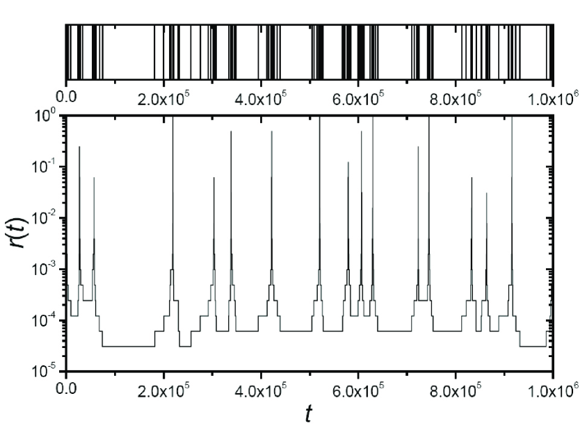
In the simulations, the initial value of is set as , which is also the possibly maximal value of in the whole simulation process. As shown in Fig. 1, the succession of events predicted by the present model exhibits very long inactive periods that separate the bursts of rapidly occurring events, and the corresponding shows a clearly seasonal property (quasi-periodic behavior). Actually, in a period, the maximal and minimal values of respectively determined by and as and . This quasi-periodic property will be applied in the further analysis. Note that, in a specific quasi-period, can be smaller than and can be smaller than . It is because could happen when and could happen when .
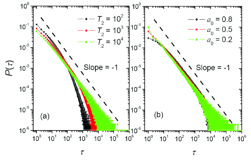
Figure 2 reports the simulation results with tunable and . Given , if , the interevent time distribution generated by the present model displays a clearly power law with exponent -1; while if is not sufficiently large, the distribution exhibits a departure from a power-law form with a cut-off in its tail. Correspondingly, given sufficiently large , the effect of is very slight, thus can be ignored.
Taking into account the quasi-periodic property of , we raise two approximated assumptions before analytical derivation: (i) The statistical property of is the same as that in a single period; (ii) Within one period, the statistical property of in the -increasing half is the same as that in the -decreasing half. In the reducing process, , where . The integer denotes the number of the events in the reducing process (also the number of different values of ), whose value is about
| (2) |
since and . is the initial value (it is also the maximum value) of in a reducing process. Note that, for different reducing processes, the values of are not always the same. Though has the same order of magnitude with , its value can be less than in a specific process. The average value of will be calculated later in this paper.
If the current occurring probability is , the probability that the next event will happen at the time is:
| (3) |
Considering every value of in the reducing process, the interevent time distribution of the reducing process is:
| (4) |
According to the approximated assumptions above, the interevent time distribution of all the successions can also be expressed by Eq. (4), which can be approximately rewritten in a continuous form, as:
| (5) |
Therefore, can be further expressed as:
| (6) |
From Eq. (6), for a fixed , when is large enough (it is equivalent to the condition ), has a power-law tail with exponent -1. In addition, this analytical result also provides an explanation about the departure from a power law when is not sufficiently large.
As discussed before, for different reducing processes of , the possible values of are not always the same (see also the lower panel of Fig. 1: for different quasi-periods, the maximum values of are different). Since the order of magnitude of is comparable with (it is equal to ), the minimum value of , , has the same order of magnitude with . Making the approximated assumption that the minimum value of is given by in a -increasing process, and the maximum value of in the next -decreasing process is ( is also the start point in the next decreasing process), then the probability density of reads
| (7) |
Therefore, the average value of is
| (8) |
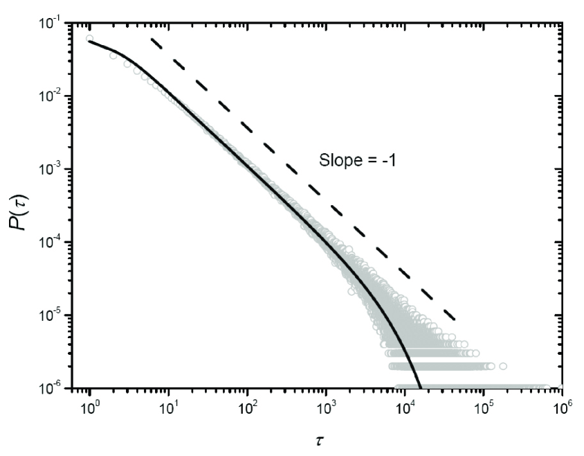
This average value of calculated by Eq. (8), as well as the integer part of (as the approximation of ), can be directly used in the approximate calculations of Eq. (6). Given , , and , one obtains , and by Eq. (8). Accordingly, Fig. 3 reports the comparison of analytical and simulation results, which are well in accordance with each other.
IV CONCLUSION AND DISCUSSION
A novel model on human dynamics is proposed in this paper. Different from the mainstream queuing models, the current model is driven by the personal interests. In this model, the frequency of events are determined by the interest, while the interest are simultaneously affected by the occurrence of events. This interplay working mechanism, similar to the active walk Lam2005 ; Lam2006 , is a genetic origin of complexity of many real-life systems. The rules in the current model are extracted from our daily life, and both the analytical and simulation results agree well with the empirical observation, such as the activity pattern of web browsing Dez6 . Our work indicates a simple and universal mechanism in human dynamics, that is, a people could adaptively adjust their interest on a specific behavior (e.g. watching TV, browsing web, playing on-line game, etc.), which leads to a quasi-periodic change of interest, and this quasi-periodic property eventually gives raise to the departure of Poisson statistics.
Besides the HPF protocol and the current model, there are also some other mechanisms that can lead to a power-law interevent time distribution. For example, Hidalgo Hidalgo2006 pointed out that a Poissonian individual with characteristic time varying randomly in time could generate a power-law interevent time distribution with exponent -2. In addition, Vázquez Vazquez2007 showed that if the current executing rate is linearly correlated with the average executing rate in a immediate predecessor period, the interevent time distribution will follow a power-law form.
Note that, although in the recent empirical works, the power-law form is widely used to fit the interevent time distribution of human behaviors, there exists a debate about the choice of fitting functions for this distribution in the e-mail communication Stouffer2005 ; Barabasi2005 . Actually, a candidate, namely log-normal distribution, has also been suggested Stouffer2005 to describe the non-Poisson temporal statistics of human activities. The stretched exponential distribution Laherrere1998 ; Zhang2006 , interpolating between a power law and an exponential form, serves as another candidate (see, for example, the distribution of interevent time between two consecutive transactions initiated by a stock broker Vqz10 ). A clear understanding of the tails in the interevent time distribution asks for in-depth exploration on empirical data in the future.
The concept and methodologies related to the statistics of the interevent time can also find its applications in some other systems. For example, similar statistical analysis can be addressed on the spacing between the consecutive occurrences of the same letter in written text Goh2008 , and the time difference between successive events above a certain threshold (i.e., extreme events) Bogachev2007 .
Finally, we point out some limitations in the current model. Firstly, it can only generate the power-law interevent time distribution with exponent -1, which does not agree with some real human-initiated systems with different power-law exponents. Secondly, we assume that the changing rate of the occurring probability, , is fixed as a constant in every rising or decaying process. This assumption is very ideal, and we could not find any support from the empirical data. Third, as stated by Kentsis Kentsis2006 , there are countless ingredients affecting the human dynamics, and for most of them, we do not know their impacts. Those ingredients, such as the social content, the semantic content and the periodicity due to circadian and weekly cycles, have not been considered in the present model, neither the HPF protocol. However, although this model is rough and may contain some artificial assumptions, it provides a start point of modeling interest-based human dynamics. The human-initiated systems are the most complex systems, and there must be many underlying mechanisms having not been discovered yet. We believe our model could highlight the readers in this rapidly growing area.
Acknowledgements.
We acknowledge the the useful discussion with Wei Hong and Shuang-Xing Dai, this work is partially supported by the National Natural Science Foundation of China (Grant Nos. 10472116 and 10635040), and the 973 Program 2006CB705500.References
- (1) J. B. Watson, Psychological Review 20, 158 (1913).
- (2) F. A. Haight, Handbook of the Poisson Distribution (Wiley, New York, 1967).
- (3) A. -L. Barabási, Nature (London) 435, 207 (2005).
- (4) J. G. Oliveira, and A. -L. Barabási, Nature (London) 437, 1251 (2005).
- (5) K. -I. Goh, and A. -L. Barabási, EPL 81, 48002 (2008).
- (6) T. Zhou, X. -P. Han, and B. -H. Wang, arXiv: 0801.1389.
- (7) V. Plerou, P. Gopikrishnan, L. A. N. Amaral, X. Gabaix, and H. E. Stanley, Phys. Rev. E 62, 3023(R)(2000).
- (8) J. Masoliver, M. Montero, and G. H. Weiss, Phys. Rev. E 67, 021112 (2003).
- (9) Z. Dezsö, E. Almaas1, A. Lukács, B. Rácz, I. Szakadát, and A. -L. Barabási, Phys. Rev. E 73, 066132 (2006).
- (10) T. Zhou, H. A. -T. Kiet, B.J. Kim, B. -H. Wang, and P. Holme, EPL 82, 28002 (2008).
- (11) W. Hong, X.- P. Han, T. Zhou, and B. -H. Wang, arXiv: 0802.2577.
- (12) A. Vázquez, Phys. Rev. Lett. 95, 248701 (2005).
- (13) A. Vázquez, J. G. Oliveira, Z. Dezsö, K. -I. Goh, I. Kondor, and A. -L. Barabási, Phys. Rev. E 73, 036127 (2006).
- (14) T. Henderson, and S. Nhatti, Proc. 9th ACM Int. Conf. on Multimetia, pp. 212 (ACM Press, 2001).
- (15) L. Lam, Int. J. Bifurcation & Chaos 15, 2317 (2005).
- (16) L. Lam, Int. J. Bifurcation & Chaos 16, 239 (2006).
- (17) C. Hidalgo, Physica A 369, 877 (2006).
- (18) A. Vázquez, Physica A 373, 747 (2007).
- (19) D. B. Stouffer, R. D. Malmgren, and L. A. N. Amaral, arXiv: physics/0510216.
- (20) A. -L. Barabási, K. -I. Goh, and A. Vázquez, arXiv: physics/0511186.
- (21) J. Laherrere and D. Sornette, Eur. Phys. J. B 2, 525 (1998).
- (22) P. P. Zhang, K. Chen, Y. He, T. Zhou, B. B. Su, Y. D. Jin, H. Chang, Y. P. Zhou, L. C. Sun, B. H. Wang, D. R. He, Physica A 360, 599 (2006).
- (23) M. I. Bogachev, J. F. Eichner, and A. Bunde, Phys. Rev. Lett. 99, 240601 (2007).
- (24) A. Kentsis, Nature (London) 441, E5 (2006).