Modeling microevolution in a changing environment: The evolving quasispecies and the Diluted Champion Process
Abstract
Several pathogens use evolvability as a survival strategy against acquired immunity of the host. Despite their high variability in time, some of them exhibit quite low variability within the population at any given time, a somehow paradoxical behavior often called the evolving quasispecies. In this paper we introduce a simplified model of an evolving viral population in which the effects of the acquired immunity of the host are represented by the decrease of the fitness of the corresponding viral strains, depending on the frequency of the strain in the viral population. The model exhibits evolving quasispecies behavior in a certain range of its parameters, and suggests how punctuated evolution can be induced by a simple feedback mechanism.
pacs:
87.23.kg,87.10.Mn1 Introduction
Pathogenic viruses, in order to survive and successfully reproduce have to fight against the immune system of their host organisms. Some viruses use evolvability as a successful strategy to escape acquired immunity. In the presence of adaptive response in the host newly arising mutants can acquire a competitive advantage with respect to the wild type. Neverthless, in some viral populations one often observes “quasispecies” behavior, in which individuals are strongly similar to one another.
A prototypical example of this behavior is exhibited by the Influenza A virus, which makes use of high antigenical variability (genetic drift) to escape acquired immune response. Virus strains circulating in different epidemic seasons, in spite of eliciting a certain amount of cross-response by the immune system of the hosts, mutate fast enough to be able to infect the same host several times in the course of its life. However in any given observed epidemics, the viral population is sufficiently concentrated around a well defined strain that effective vaccines can be prepared. Moreover, antigenic changes are punctuated: antigenic assays show that the sequences of the dominant circulating type H3N2 fall into temporally correlated clusters with similar antigenic properties ([1]). This behavior, which has been described as an evolving viral quasispecies, contrasts with the prediction of naive models of viral evolution (see, e.g., [2]), where the interaction with the immune system leads to proliferation of strains with different antigenic properties and, consequently, to the impossibility of preparing effective vaccines. It has recently been experimentally shown [3] that some bacteria in a changing environment can develop a genotype which produces highly variable phenotypes, presumably adapted to different environments. One may speculate whether such a bet-hedging strategy is available to viruses, due to the small size of their genetic material and their high mutation rate, especially for RNA-based viruses.
A different example is the one of the in-host evolution of the HIV, which exploits high mutation rates to counter the immune adaptation of its host (see, e.g., [4, 5]). Despite its high mutation and substitution rates, the viral population shows low levels of differentiation during most of the asymptomatic phase.
Several solutions have been proposed to this evolutionary puzzle, based on the analysis of mathematical models. In [6], elaborating on previous theory ([7]), it was proposed that in the case of influenza A, a short-time strain-trascending immunity could give account for the quasispecies behavior. It was observed in [8] that this short-term immunity would be ineffective in the absence of heterogeneities in infections, due either to the structure of network of infective contacts or to variations in the infective efficacy of different strains. An alternative explanation was put forward in [9] based on the analysis of a model, where the heterogeneity of the neutral phenotypic network of the evolving virus is taken into account. An important feature in influenza epidemics seems to be the directionality of its propagation. According to the analysis of [10] and [11] yearly epidemics typically start from seeds in South-East Asia before spreading worldwide. This suggests the presence of strong bottlenecks in the viral population that could lead to relatively small effective population sizes and to a strong reduction of genetic variability.
Models can suggest mechanisms that can produce the observed evolutionary pattern. However, even the simplest individual based model of viral evolution in a host population ([8]) is too complicated to lead to a detailed exploration of parameter space. It is not clear which conditions on evolutionary and epidemiological parameters allow for the evolving quasispecies behavior. In particular we will be interested to the dependence on the population size. We wish to ascertain whether in the presence of the infectivity reduction due to the immune response of the host, the quasispecies behavior can appear for some parameter ranges in the infinite population, or is only possible in sufficiently small populations. This last possibility would emphasize the importance of population bottlenecks in the ecology of the virus.
In this paper we introduce a simplified model of evolving viral population that keeps into account the interaction between virus and host immunity in an effective way. The effectiveness of reproduction of a given viral type at a given time depends on its age and its past frequency in the host population. We get a model that is simple enough to allow to study at least numerically, the dependence on the different parameters, and in particular on the population size. Our findings suggest that quasispecies behavior and punctuated equilibria are only possible for small enough populations, whereas, if the model parameters are not scaled with the population size, one always has proliferation in the large population limit.
The organization of the paper is the following: in section 2 we define our model as an extension of Kingman’s house of cards model, where strains are represented by self-reproducing entities and the immune memory of the host is taken into account by the decrease of the strain fitness with time. In this model, the fitness of a mutant is independent of that of its parental strain. This assumption is justified in our approach by the fact that since the parental fitness decreases very quickly due to the immune adaptation of the host, we do not expect long-lived fitness correlations to exist among related strains. In section 3 we recall some known results about the dynamics of the model in the absence of memory. In section 4 we study the effect of the immune memory in numerical simulations and show the existence of the evolving quasispecies regime. In 5 we analyze in more detail the behavior of the system in the evolving quasispecies regime. In 6 we introduce a simple effective stochastic process that helps in understanding the dynamical behavior of the quasispecies regime. Finally some conclusions are drawn.
2 The Model
We consider here a model of an evolving viral population of constant size consisting of individuals. The population evolves according to a Wright-Fisher process for asexually reproducing populations ([12, 13]). At each discrete time step the population reproduces and is completely replaced by its progeny. Each individual is characterized by its strain label . The expected offspring size of an individual belonging to strain is proportional to the Wrightian fitness of its strain. The fitness of a strain depends on its intrinsic fitness , proportional to its basic reproductive number, and changes with time as described below. In what follows we shall also use the notation and call the Fisher fitness of . As it is well known ([14]) the Wright-Fisher model can be described as a process where each individual at generation “chooses” its parent at generation with probability equal to . Consequently, for large , the offspring size of an individual is a random Poissonian variable with average .
At each reproduction event, a mutation can take place with probability . Upon mutation, a new strain appears, and its intrinsic fitness is drawn from a fixed probability distribution ([8, 15, 16, 17]), independently for each mutation event: this corresponds to the infinite allele approximation where no back mutations are possible. The fitness of the newly formed strain is equal to its intrinsic fitness . If fitnesses did not depend on time, the model would coincide with Kingman’s house-of-cards model ([15]).
The effect of acquired immunity of the host population on the viral reproduction is represented by letting the fitness of each strain decrease at each generation with a rate proportional to the number of individuals belonging to that strain in the population. For simplicity we consider an exponential decrease of the fitness:
| (1) |
where is a parameter which determines the rate of fitness decrease.
In the following we will describe mainly the case in which is a log-normal distribution . We have also investigated the model with the uniform fitness distribution finding the same qualitative results.
3 Dynamic behavior in the absence of immunity
We start by reviewing the behavior of the model for , i.e., in the absence of immune memory of the host ([15, 17, 18]). In this case, in the limit of large populations , it is possible to derive an exact equation for the evolution of the fraction of individuals with fitness at time , namely
| (2) |
where . The nature of the solution of this equation depends on the properties of . If has a compact support (i.e., for ), the equation admits a stationary state satisfying
| (3) |
This distribution is analogous to the Bose distribution, with playing the role of the Boltzmann factor. Therefore, if , the Einstein condensation can take place. This transition is known as the error threshold in evolutionary models, and separates a poorly adapted phase at high mutation rate from a well adapted phase at low mutation rate. In the well adapted (condensed) phase, found for , a finite fraction of the population has the maximum fitness . Here and are given by
| (4) |
In this phase the reproduction rate of the individuals with maximal fitness equals one: , while all the others have reproduction rates smaller than one. Conversely, in the poorly adapted (uncondensed) phase, less than maximally fit individuals can reproduce. If the integral is divergent no error threshold appears.
The situation where the fitness distribution extends to infinity is more complex and interesting. In this case, equation (2) does not admit a stationary solution and one obtains instead a run-away. However, in contrast with the case of compact support, the dynamics for a finite population with individuals can now be substantially different from the infinite population limit. In fact, the evolution process can be described as a non stationary record process where condensates of a given fitness are replaced by ones of higher fitness ([18]), with persistence times that becomes longer and longer as the fitness increases. It has been noticed in [17] that, however, an uncondensed phase can be metastable for long times. Let us denote by the maximum fitness appearing among the mutants in generations. As at each time step a number of new mutants appear, the maximum fitness for one generation satisfies
| (5) |
If the reproduction rate is smaller than one, the uncondensed phase will be stable. This quantity depends on via the average . Then the stability time can be determined by the condition that the maximal fitness of mutants over an interval of generations, as determined by the relation has a reproduction rate equal to one. In this way one gets an effective - and - dependent error threshold, which can be approximately described by equations
| (6) |
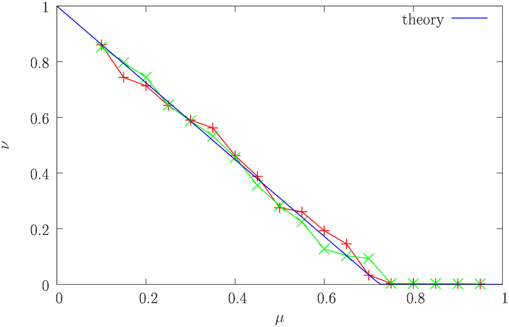
In figure 1 we compare this analysis with numerical simulations for the lognormal distribution with parameter , showing the fraction of the condensate for two independent populations of individuals evolving for generations, together with the predictions of equation (6) as a function of the mutation rate.
4 Introducing the fitness decay
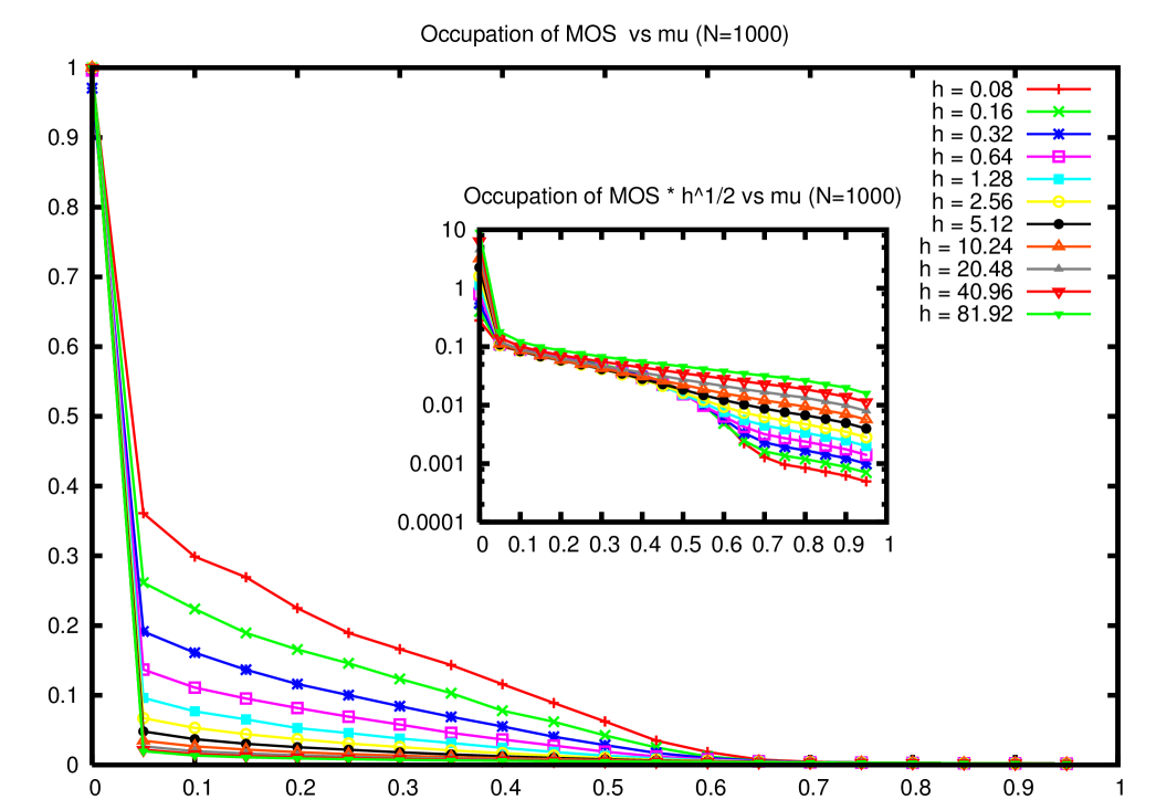
Let us now study the effect of the fitness decay and set . We continue to dwell mainly on the case of lognormal fitness distribution with parameter . In order to study the possibility of a non zero condensate we observe that while for the maximally occupied genome should usually coincide with the one of highest fitness, this is not necessarily true if . Let us define therefore, at any given time, the leader strain in the population as the one that is populated by the largest fraction of individuals, and the max as the one whose fitness is largest. In figure 2 we plot the occupation fraction of the leader as a function of the mutation rate, for several values of , in a population of size . The figure shows that while the leader occupation fraction is a decreasing function of , the error threshold is not destroyed by the immunity response and the critical value is roughly independent of .
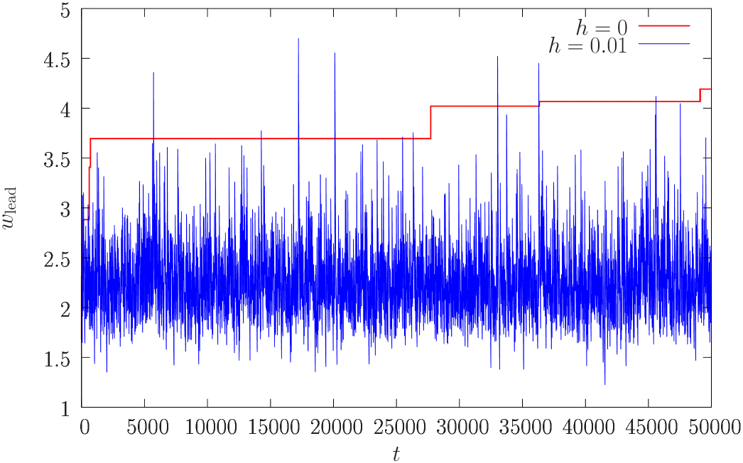
We also observe that a non zero introduces a natural time scale into the system, and one should expect that stationarity is reached after a finite relaxation time, so that the critical value of becomes time independent. In figure 3 we compare the fitness of the leader as a function of time in the condensed phase for to the one corresponding to a small value of . One can manifestly see that while stationarity does not hold in the former case, it holds in the latter.
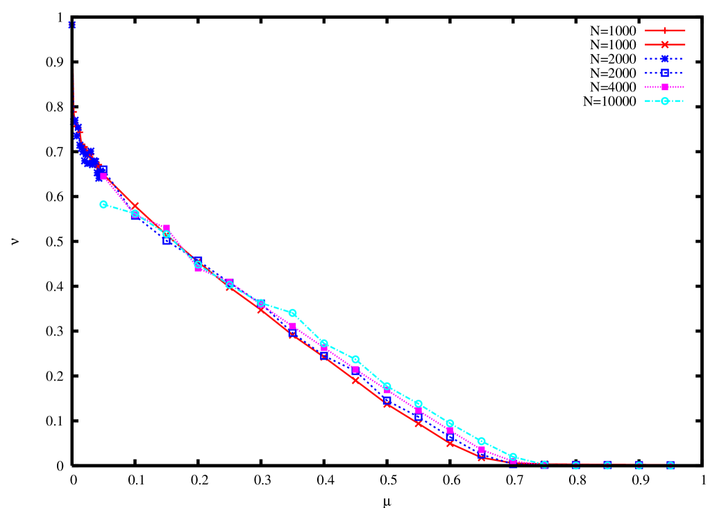
In figure 4 we plot the occupation of the leader as a function of the mutation rate for various values of . One can see that the error threshold slowly moves to higher values of as increases.
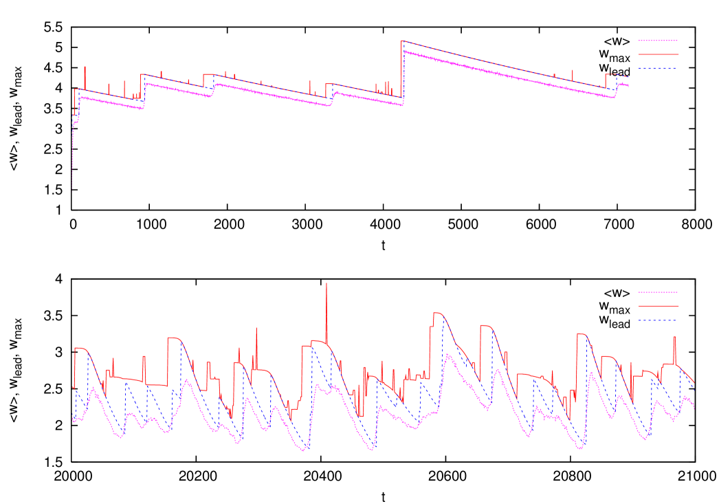
This also appears in the behavior of the leader fitness and of the maximal fitness in the system which exhibit a maximum at the error threshold. We plot these quantities together with the average fitness in figure 5. In order to obtain a less cluttered plot, the fitnesses are rescaled by the factor , where is the width of the distribution of , expected on the basis of extreme-value statistics for the lognormal distribution. The range of variation of this factor is too small to warrant drawing any conclusion from this observation. Notice that while the leader and the maximal fitnesses reach the maximum at the error threshold, the average fitness has a maximum at a lower value of .
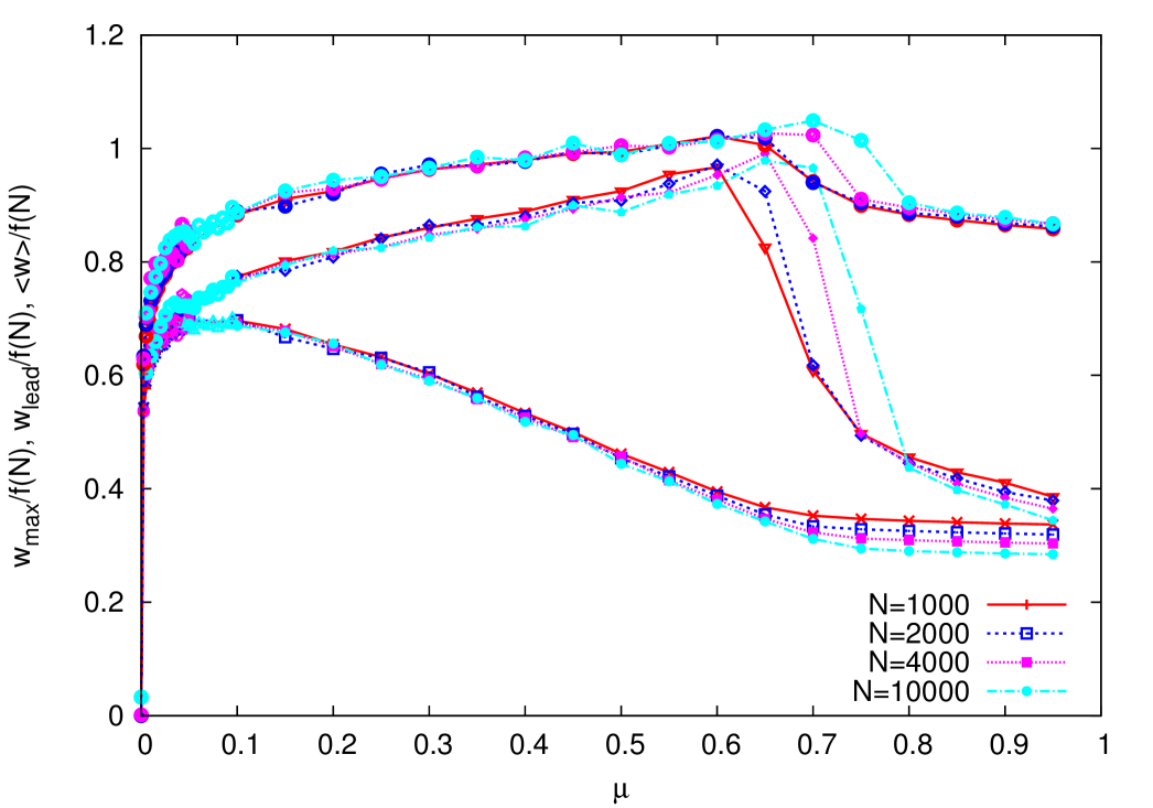
Close to the maximum of the average fitness the leader and the max occupation fractions turn out to be roughly independent of , as it can be seen from figure 6, which plots these two quantities as a function of . Conversely, figure 7 shows that the fitness of the leader and of the max are functions of : for larger a proportionally larger is needed to decrease the fitness of the same amount.
5 Dynamics
The results of the previous section clearly show that the error threshold persists even in the presence of a small amount of immune response in the host. In order to gain a better understanding of the evolving quasispecies regime characterizing the well adapted phase, let us look at the temporal behavior of the system. In figure 8 we show the occupation fractions of the max and of the leader as a function of time, in the well adapted phase with and in a population of individuals. We can see that both quantities exhibit a regular behavior in time, which can be qualitatively described as follows. When a new fitter mutant establishes in the population, it substitutes the previous leader and remains leader for a while before being at his turn substituted. We find therefore a kind of punctuated equilibrium dynamics, as announced in the introduction.
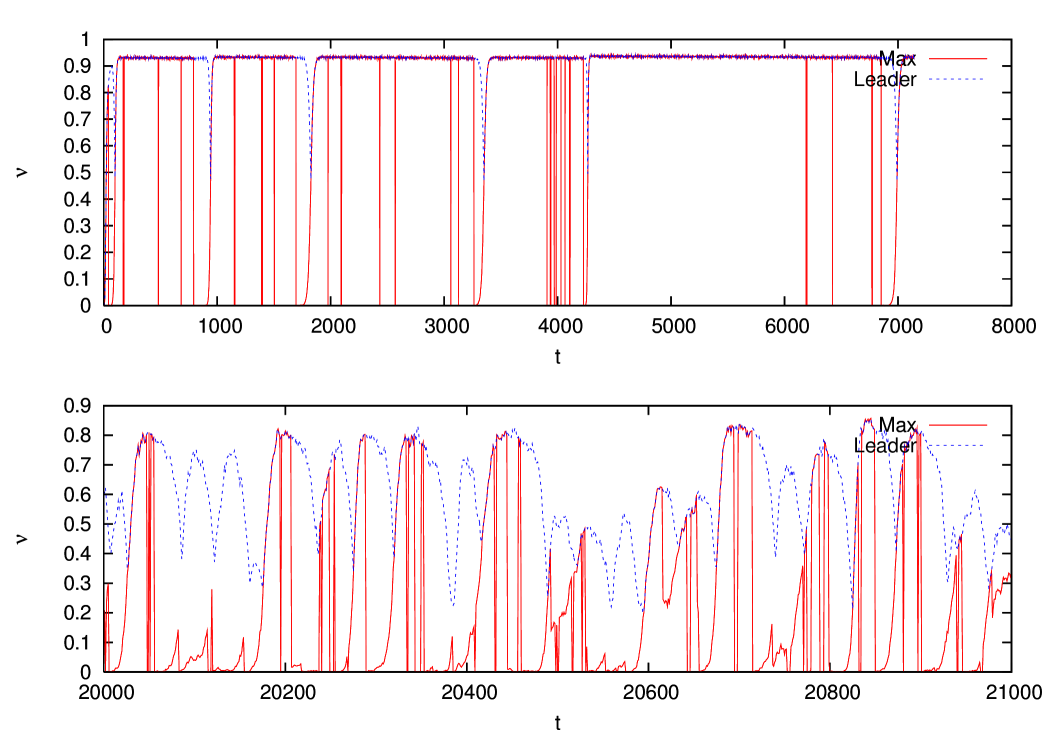
Figure 9 shows the corresponding behavior of the average fitness of the leader and of the max respectively. One sees that the fitness of the max stays constant for a while after the emergence of the mutant, and then, when the max replaces the leader, it rapidly decreases until a new leader takes over.
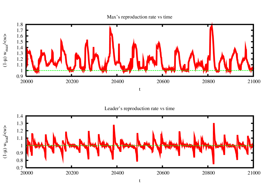
It is interesting to look at the reproduction rate of the leader strain. As shown in figure 10, this is observed to differ substantially from one only close to substitution events. Just before substitution, the challenged leader has a reproduction rate which is smaller than one, while it is larger then one just after substitution. In the periods when the leader largely dominates the population (dominance periods) the reproduction ratio is very close to one, and diversity in the population is maintained by mutants.
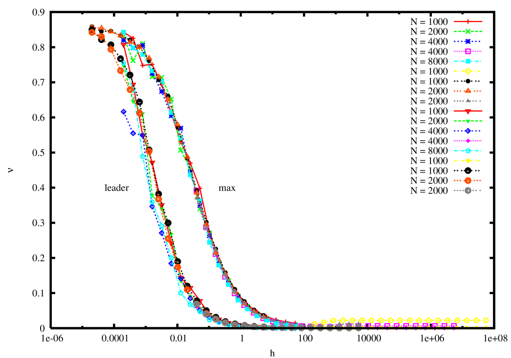
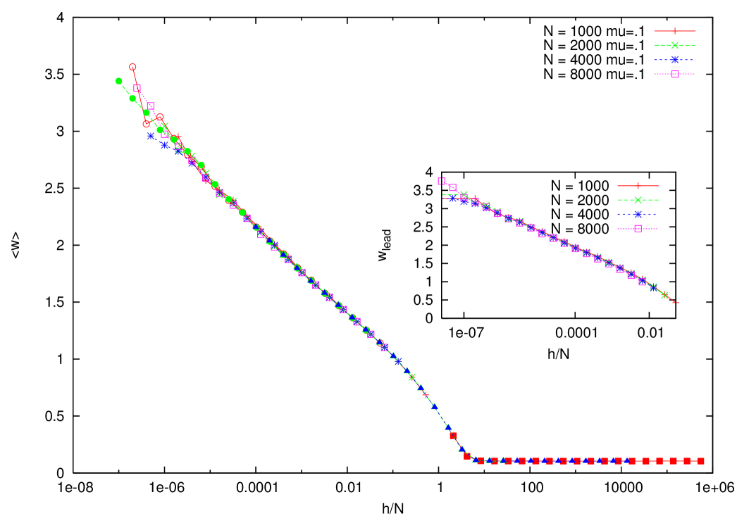
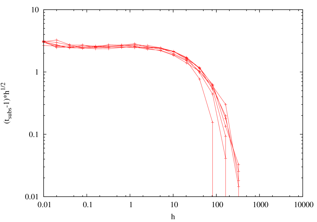
We measured the average duration of the leadership, i.e., the time interval between successive substitutions. In figure 11 we plot vs. , showing that this quantity it is roughly proportional to , and essentially independent of , in the quasispecies regime. Given the natural decay time of fitness on time scales of order it would have been natural to hypothesize a substitution time of the same order. Our numerical result show that substitutions being separated by times of order are much more frequent.
6 The Diluted Champion Process
Certain aspects of the evolving quasispecies dynamics at low and can be interpreted by introducing an effective stochastic process for the substitution. We start by defining the Champion Process where at each time there is a leader. The performance of the leader, which is represented by a fitness value, declines exponentially in time: with . The leader is challenged at regular intervals of time, and the challenger’s fitness is extracted randomly from a distribution . If the fitness of the challenger exceeds the one of the leader in charge, the challenger substitutes the old leader. Otherwise there is no substitution and the old champion remains in charge. The Diluted Champion Process (DCP) is a simple variation of the process where the substitution process is not deterministic. Substitutions can occur with a certain probability that depends on the fitness ratio between the challenger and the champion in charge. This model can obviously be adapted to competition situations where the performances of the individuals naturally decline in time.
Now, in the evolving quasispecies regime of our model, while the substitution times and the leaders fitnesses are random quantities, the dynamics between punctuations is essentially deterministic. Moreover, the champion substitution process requires times that are much shorter than the typical times of change of the fitness. Indeed as figures 8 and 9 show, the fitness of the champion starts to decay as soon as the new challenger takes over. These observations make the DCP description pertinent for our model. During the dominance periods, at each time step the champion is challenged by a number of mutants Poisson distributed with , with random fitnesses drawn from . By elementary extreme values statistics, the best fit challenger has therefore a fitness distribution given by . This will have a fixation probability , which can be estimated by the Kimura expression: . Thus the probability of survival in one round of a leader with fitness is given by
| (7) |
At this point we will assume, consistently with the simulations, that for small we can neglect the fixation time with respect to the leader strain lifetime, and suppose that for a champion , with a constant equal to where is the condensate fraction. In the case of the DCP, one can safely assume , leading to .
It is possible to formally write the basic formula for the probability that a champion with initial fitness is substituted after exactly time steps by a new champion with fitness , namely:
| (8) |
From this equation all the the properties of the DCP can be in principle derived. One can express the conditional probability that the leader fitness equals given the previous leader fitness by
| (9) |
Then one can in principle obtain the stationary distribution of the leader fitness from
| (10) |
and the distribution of the substitution time at stationarity from
| (11) |
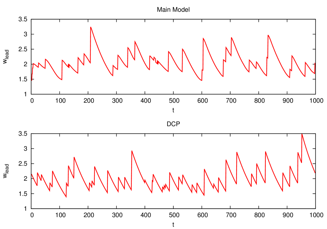
Unfortunately these equations are not easily analyzed, so in order to test the validity of this simple effective model we had to simulate it. In figure 12 we show the typical evolution of the leader’s fitness as a function of time. The DCP clearly reproduces the qualitative features of our model.
7 Conclusions and perspectives
We have introduced a simple effective model describing the evolution of a population of pathogens in the presence of the immunological response of the host. The model is simple enough to be amenable to a systematic numerical investigation, and allows one to identify a parameter region in which the coexistence of a well-defined quasispecies and of a fast turnover of the dominant strain is be quite robust. The behavior of the model in this region can be understood in terms of a further simplified model: the Diluted Champion Process. Our model can be interpreted in several ways: on the one hand, as describing the evolving viral strains present in the host population, e.g., in the case of the annual influenza epidemics; on the other hand, as the evolution of the viral population in a chronic infection of a single host individual, as in intra-host HIV evolution. In this case, fluctuations in the strength of immune response could cause proliferation of the number of strains and then the failure of the immunity system to downregulate all the viral strains (see, e.g., [19]). It is possible to obtain a more realistic description of this regime by, e.g., relaxing the fixed population constraint. It is also possible to consider a higher degree of correlation in the fitness landscape, in order to understand the extent of the stability of the punctuated equilibrium regime.
We are working on a generalization of our model taking into account the existence of different regions. They can be understood as different climatic regions in the case of epidemics, or localization in different organs in the case of intra-host infection. This investigation will allow us to understand better the different roles played by different regions: seeder, reservoirs, etc., as observed in recent analyses of epidemiological data collected in the last years ([10, 11]), or to identify possible gene-surfing phenomena in the diffusion of new strains from external regions ([20]).
References
References
- [1] Smith D J, Lapedes A S, de Jong J C, Bestebroer T M, Rimmelzwaan G F, Osterhaus A D M E and Fouchier R A M 2004 Science 305 371–376
- [2] Girvan M, Callaway D S, Newman M E J and Strogatz S H 2002 Phys. Rev. E 65 031915
- [3] Beaumont H J E, Gallie J, Kost C, Ferguson G C and Rainey P B 2009 Nature 462 90–93
- [4] Liu S L, Rodrigo A G, Shankarappa R, Learn G H, Hsu L, Davidov O, Zhao L P and Mullins J I 1996 Science 273 415–416
- [5] Shankarappa R, Margolick J B, Gange S J, Rodrigo A G, Upchurch D, Farzadegan H, Gupta P, Rinaldo C R, Learn G H, He X, Huang X L and Mullins J I 1999 J. Virol. 73 10489–10502
- [6] Ferguson N M, Galvani A P and Bush R M 2003 Nature 422 428–433
- [7] Webster R G, Bean W J, Gorman O T, Chambers T M and Kawaoka Y 1992 Microbiol. Mol. Biol. Rev. 56 152–179
- [8] Tria F, Lässig M, Peliti L and Franz S 2005 JSTAT: J. Stat. Mech.: Theory and Experiment P07008
- [9] Koelle K, Cobey S, Grenfell B and Pascual M 2006 Nature 314 1898–1903
- [10] Rambaut A, Pybus O G, Nelson M I, Viboud C, Taubenberger J K and Holmes E C 2008 Nature 453 615–619
- [11] Russell C A, Jones T C, Barr I G, Cox N J, Garten R J, Gregory V, Gust I D, Hampson A W, Hay A J, Hurt A C, de Jong J C, Kelso A, Klimov A I, Kageyama T, Komadina N, Lapedes A S, Lin Y P, Mosterin A, Obuchi M, Odagiri T, Osterhaus A D M E, Rimmelzwaan G F, Shaw M W, Skepner E, Stohr K, Tashiro M, Fouchier R A M and Smith D J 2008 Science 320 340–346
- [12] Wright S 1931 Genetics 16 97–159 reprinted in Bull. Math. Biol. 52, 241–295 (2006)
- [13] Fisher R A 1930 The Genetical Theory of Natural Selection (Oxford University Press) reprinted 1958: Dover Publications, New York
- [14] Derrida B and Peliti L 1991 Bull. Math. Biol. 53 355–382
- [15] Kingman J F C 1978 J Appl Prob 15 1–12
- [16] Franz S and Peliti L 1997 J. Phys. A: Math. Gen. 30 4481
- [17] Neher R A and Shraiman B I 2009 Proc. Natl. Acad. Sci. USA 106 6866–6871
- [18] Park S C and Krug J 2008 JSTAT: J. Stat. Mech.: Theory and Experiment P04014
- [19] Nowak M A 1995 J. Acq. Imm. Def. Syndr. and Human Retrovir. 10 S1–S5
- [20] Hallatschek O and Nelson D R 2007 Theor. Pop. Biol. 158–170