Modeling of Cosmic-Ray Production and Transport and Estimation of Gamma-Ray and Neutrino Emissions in Starburst Galaxies

A starburst galaxy (SBG) is characterized by a nuclear region, named as the starburst nucleus (SBN), with enhanced star formation rate (SFR) (e.g., Kennicutt & Evans, 2012, and references therein). Young massive stars blow powerful stellar winds (SWs) throughout their lifetime and die in spectacular explosions as core-collapse supernovae (SNe) (Weaver et al., 1977; Freyer et al., 2003; Georgy et al., 2013; Janka, 2012). Various shock waves driven by these activities can accelerate cosmic-rays (CRs) primarily through diffusive shock acceleration (DSA) (e.g., Drury, 1983). Some of mechanical energy of SWs is expected to be converted to CRs at termination shocks in stellar wind bubbles and superbubbles created by young star clusters, colliding-wind shocks in binaries of massive stars, and bow shocks of massive runaway stars (e.g., Casse & Paul, 1980; Cesarsky & Montmerle, 1983; Bykov, 2014). Seo et al. (2018), for instance, estimated that the energy deposited by SWs could reach up to $\sim 25\%$ of that from SNe in our Galaxy. In SBGs, the relative contribution of SWs could be more important, since the the integrated galactic initial mass function (IGIMF) seems to be in general flatter for higher SFR (e.g., Palla et al., 2020; Weidner et al., 2013; Yan et al., 2017). Supernova remnant (SNR) shocks driven by core-collapse SNe propagate into the pre-SN winds with $\rho\propto r^{-2}$ density profile and strong magnetic fields, so the blast waves do not decelerate significantly and the maximum energy of CR nuclei accelerated by such shocks could reach up to $\sim 100$ PeV (e.g., Berezhko & Völk, 2000; Zirakashvili & Ptuskin, 2018). Hence, the SBNs of SBGs have been recognized as sites of very active CR production (e.g., Peretti et al., 2019; Bykov et al., 2020).

In addition, the collective input of massive SWs and SN explosions can induce supersonic outflows in SBGs, known as SBN winds, and create superwind bubbles around the SBN. It has been proposed that the termination shocks of the superwind and bow shocks formed around gas clouds embedded in the outflows can provide additional sources of the CR acceleration (Romero et al., 2018; Müller et al., 2020). In this study, we focus on the CR acceleration at shocks induced by SWs and SNRs inside the SBN (see Figure 1).

The beauty of the original DSA predictions lies in the simple power-law (PL) momentum distribution, $f_{p}(p)\propto p^{-q}$, in the test-particle regime, where the PL slope, $q=4M_{\rm s}^{2}/(M_{\rm s}^{2}-1)$, depends only on the shock sonic Mach number, $M_{\rm s}$ (e.g., Drury, 1983, and see further discussions in Section 2.1). According to the nonlinear theory of DSA, however, with a conversion efficiency of order of 10 % from the shock kinetic energy to the CR energy at strong shocks, the dynamical feedback of CR protons (CRPs) may lead to a substantial concave curvature in their momentum distribution (e.g., Berezhko & Ellison, 1999; Caprioli et al., 2009; Kang, 2012; Bykov et al., 2014). On the other hand, the time-integrated, cumulative CRP spectra produced during the SNR evolution seem to exhibit smaller concavities, compared to the instantaneous spectra at the shock position at a given age (e.g., Caprioli et al., 2010; Zirakashvili & Ptuskin, 2012; Kang, 2013). The caveat here is that the physics of DSA has yet to be fully understood from the first principles in order to make quantitative predictions (e.g. Marcowith et al., 2016). In this study, in addition to the canonical single PL form, we adopt double PL momentum spectra to represent slightly concave spectra of CRPs that might be produced by an ensemble of SNRs with wide ranges of parameters at different dynamical stages.

The CRPs in the SBN can inelastically collide with background thermal protons ($pp$ collisions) and produce neutral and charged pions, which decay into $\gamma$-rays and neutrinos, respectively. Indeed, $\gamma$-rays from SBGs have been observed using Fermi-LAT (e.g., Abdo et al., 2010; Acero et al., 2015; Peng et al., 2016; Abdollahi et al., 2020) and ground facilities, such as H.E.S.S. and Veritas (e.g., VERITAS Collaboration et al., 2009; Acero et al., 2009; The VERITAS Collaboration et al., 2015; H. E. S. S. Collaboration et al., 2018), proving the active acceleration of CRPs in SBGs. Although SBGs have not yet been identified as point sources of neutrinos, they have been considered to be potential contributors of high energy neutrinos observable in IceCube (e.g., Loeb & Waxman, 2006; Murase et al., 2013; Tamborra et al., 2014; Bechtol et al., 2017; Ajello et al., 2020). Adopting a scaling relation between $\gamma$-ray and infrared luminosities, for instance, Tamborra et al. (2014) estimated the $\gamma$-ray background and the diffuse high-energy neutrino flux from star-forming galaxies (SFGs) including SBGs, and suggested that SBGs could be the main sources of IceCube neutrinos. Bechtol et al. (2017), on the other hand, argued that considering the contribution from blazers, SFGs may not be the primary sources of IceCube neutrinos (see also Ajello et al., 2020). In addition, Peretti et al. (2020) argued that SBGs would be hard to be detected as point neutrino sources in IceCube.

There have been previous studies to explain the observed spectra of SBGs in $\gamma$-rays (as well as in other frequency ranges) and to predict neutrino emissions (e.g., Wang & Fields, 2018; Sudoh et al., 2018; Peretti et al., 2019, 2020; Krumholz et al., 2020, for recent works). The hadronic process for the production of $\gamma$-rays and neutrinos is governed mainly by the “production” and “transport” of CRPs. In most of these previous studies, CRPs are assumed to be produced at SNR shocks, and the cumulative momentum distribution of CRPs inside the SBN is described with the single PL spectrum ($\propto p^{-\alpha}$); the Fermi-LAT $\gamma$-ray observations for well-studied SBGs, such as M82, NGC253, and Arp220, require the CRP momentum distribution with $\alpha\sim 4.2-4.5$.

The transport of CRPs in the SBN is expected to be regulated by the advection due to the superwinds escaping from the SBN and the diffusion mediated by magnetic turbulence. The wind transport is energy-independent and the advection time-scale of CRPs would be comparable to the energy loss time-scale, $\tau_{\rm loss}(p)$, in SBGs (e.g., Peretti et al., 2019). On the contrary, the diffusive transport is expected to depend on the CRP energy. It has been modeled, for instance, with the large-scale, Kolmogorov-type turbulence of $\delta B/B\sim 1$ expected to be present in the interstellar medium (ISM) (e.g., Sudoh et al., 2018; Peretti et al., 2019), and then for most CRPs, the diffusion time-scale, $\tau_{\rm diff}(p)\sim L^{2}/D(p)$, is longer than $\tau_{\rm loss}(p)$ (see Figure 3 below). Krumholz et al. (2020), on the other hand, argued that the turbulence of scales less than the gyroradius of CRPs with $E_{\rm CR}\lesssim{\rm several}\times 0.1~{}{\rm PeV}$ would be wiped out by ion-neutral damping, and suggested that CRPs interact mostly with the Alfvén waves that are self-excited via CRP streaming instability. With this model, in the energy range of $E_{\rm CR}\gtrsim 1~{}{\rm TeV}$, $\tau_{\rm diff}(p)\ll\tau_{\rm loss}(p)$, so CRPs are inefficiently confined in the SBN.

Previous studies have been successful to some degree in modeling the production and transport of CRPs in SBGs and reproducing/predicting $\gamma$-ray and neutrino emissions from them. In this work, we expand such efforts; we consider different models for CRP production and transport, and estimate $\gamma$-ray and neutrino emissions for nearby SBGs, specifically, M82, NGC253, and Arp220. First, in addition to the single PL momentum distribution, we consider the double PL distribution for SNR-produced CRPs. This is partly motivated by the employment of double PLs in fitting observed $\gamma$-ray spectra (e.g., Tamborra et al., 2014; Bechtol et al., 2017), but also by the consideration of nonlinear DSA theory as discussed above. We also consider the CRPs produced at SW shocks. Second, we adopt different diffusion models for the diffusive transport of CRPs in the SBN, specifically the model where CRPs scatter off the Kolmogorov turbulence of $\delta B/B\sim 1$ and the model suggested by Krumholz et al. (2020). We then examine the consequence of different momentum distributions of CRPs, combined with different diffusive transport models in the estimation of $\gamma$-ray and neutrino emission from SBGs. Finally, we discuss the implications of our results.

In this study, we consider the $\gamma$-rays and neutrinos emitted from the SBN only (see also, e.g., Peretti et al., 2019, 2020), while ignoring the contribution from the galactic disk. Since both the gas density and CRP density should be substantially lower in the disk than in the SBN, the disk would make relatively a minor contribution.

This paper is organized as follows. In Sections 2 and 3, we detail models for the production and transport of CRPs in the SBN. In Sections 4 and 5, we present the estimates of $\gamma$-rays and neutrinos from SBGs. A summary including the implications follows in Section 6.

Following the simple approach adopted in previous studies (references in the introduction), we assume that the production of CRPs is balanced by the energy loss, SBN wind advection, and diffusion. Then, the momentum spectrum of the CRP density in the SBN, $f_{p}(p)$, is given as

The energy loss is mostly due to ionization, Coulomb collisions, and inelastic $pp$ collisions, and for its time-scale $\tau_{\rm loss}$, we use the formulae in Peretti et al. (2019). The wind advection time-scale, $\tau_{\rm adv}$, is calculated as the radius of the SBN divided by the escaping speed of the SBN wind, i.e., $R_{\rm SBN}/v_{\rm SBNwind}$ with $R_{\rm SBN}$ and $v_{\rm SBNwind}$ given in Table 1. Figure 3 shows $\tau_{\rm loss}$ (magenta solid line) and $\tau_{\rm adv}$ (black dashed line) estimated for M82; the two time-scales are comparable.

For the diffusion time-scale $\tau_{\rm diff}$, we consider two different diffusion models. First, we adopt the model A of Peretti et al. (2019), where CRPs scatter off the large-scale Kolmogorov turbulence in the SBN (hereafter, the diffusion model A). Then, the diffusion coefficient is given as

where $r_{g}(p)$ is the gyroradius of CRPs and the speed of CRPs is assumed to be $c$. $\mathcal{F}(k)$ is the normalized energy density of turbulent magnetic fields per unit logarithmic wavenumber, which is defined as

with $k_{0}=1~{}{\rm pc}^{-1}$. Note that 1 pc is about the gyroradius of CRP of 100 PeV in the background magnetic field of 100 $\mu$G. The diffusion time-scale is given as $\tau_{\rm diff}=R_{\rm SBN}^{2}/D_{\rm A}(p)$ with the radius of the SBN. We point that $r_{g}(p)\propto p$, and $\mathcal{F}(k)\propto k^{-2/3}\propto p^{2/3}$ assuming that CRPs interact with the resonant mode corresponding to the gyroradius, and then $\tau_{\rm diff}\propto p^{-1/3}$. Peretti et al. (2019) also considered the Bohm diffusion, for which $D(p)\sim r_{g}(p)c\propto p$ and $\tau_{\rm diff}\propto p^{-1}$. But they argue that the Bohm diffusion essentially gives the same results as the Kolmogorov diffusion for the transport of CRPs, because the SBN wind advection has a shorter time-scale over most of the momentum range (see Figure 3) and so those diffusions are subdominant. Hence, we here consider only the Kolmogorov turbulence for the diffusion model A.

We also consider the diffusion model of Krumholz et al. (2020), where the CRPs of $E_{\rm CR}\lesssim 0.1$ PeV resonantly scatter off self-excited turbulence, assuming that the ISM turbulence of scales less than the gyroradius of CRPs with $\lesssim 0.1~{}{\rm PeV}$ is wiped out by ion-neutral damping (hereafter, the diffusion model B). Assuming that the turbulence is trans or super-Alfvénic, the diffusion coefficient is given as

where $v_{\rm st}$ is the CRP streaming speed, $\ell\approx\ell_{0}/M_{\rm A,turb}^{3}$, $\ell_{0}$ is the outer scale of the turbulence, and $M_{\rm A,turb}$ is the Alfvén Mach number of the turbulence. Following Krumholz et al. (2020), $\ell_{0}=H_{\rm gas}$, i.e., the gas scale height listed in Table 1, is used, and $M_{\rm A,turb}=2$ is assumed. And $v_{\rm st}$ is modeled as ($v_{\rm st}/v_{\rm Ai}-1)\propto{(E_{\rm CR}/{\rm GeV})}^{\alpha-3}$, where $v_{\rm Ai}$ is the ion Alfvén speed given in Table 1 and $\alpha$ is the PL slope of CRP momentum distribution, $\alpha_{\rm SN}$ or $\alpha_{\rm SW}$, described in Section 2. The proportional constant for different SBGs can be found in Table 1 of Krumholz et al. (2020). The diffusion time-scale is given as $\tau_{\rm diff}=H_{\rm gas}^{2}/D_{\rm B}(p)=M_{\rm A,turb}^{3}H_{\rm gas}/v_{\rm st}$.

Figure 3 compares $\tau_{\rm diff}$ to $\tau_{\rm loss}$ and $\tau_{\rm adv}$ for M82. In the estimation of $\tau_{\rm diff}$ of the diffusion model B in the figure (blue solid line), the single PL momentum distribution of SNR-produced CRPs only with $\alpha_{\rm SN}=4.25$ is used. The slope of $\tau_{\rm diff}(p)$ is $(3-\alpha_{\rm SN})$ in the range of $p\sim 1-100$ TeV/$c$ for the diffusion model B. With the diffusion model A, the energy loss and wind advection dominate over the turbulent transport, except at the highest momentum of $p\gtrsim 10$ PeV/$c$. In the case of the diffusion model B, on the other hand, $\tau_{\rm diff}$ becomes shorter than $\tau_{\rm loss}$ or $\tau_{\rm adv}$ for $p\gtrsim 1$ TeV/$c$, so high energy CRPs are confined within the SBN for shorter time and have less chance for collisions with background thermal protons. The kink in $\tau_{\rm diff}$ of the diffusion model B appears at $p\sim 0.1$ PeV/$c$, because the momentum-dependent streaming velocity becomes greater than the speed of light. Hence, the model stops being valid at $p\gtrsim 0.1$ PeV/$c$; the CRPs in this high momentum range may interact with the large-scale turbulence in the SBN, resulting in longer $\tau_{\rm diff}$. This may affect in particular the estimation of neutrino emission in $E_{\nu}\gtrsim 10$ TeV (see Section 5 for further comments).

With the CRP momentum distribution function, $f_{p}(p)$, calculated in Equation (8), we first estimate the $\gamma$-ray emission due to $pp$ collisions. As in previous studies, we use the pion source function as a function of pion energy $E_{\pi}$, presented in Kelner et al. (2006),

Here, $K_{\pi}\sim 0.17$ is the fraction of the kinetic energy transferred from proton to pion, and $n_{p}(E)$ is the CRP energy distribution, given as $n_{p}(E)dE=4\pi p^{2}f_{p}(p)dp$. And $\sigma_{\rm pp}(E)$ is the cross-section, given as $(34.3+1.88\theta+0.25\theta^{2})\times[1-(E_{\rm th}/E)^{4}]^{2}$ mb, where $\theta=\ln(E/{\rm TeV})$ and $E_{\rm th}=1.22$ GeV is the threshold energy. The $\gamma$-ray source function as a function of $\gamma$-ray energy $E_{\gamma}$ is calculated as

where $E_{\rm min}=E_{\gamma}+m_{\pi}^{2}c^{4}/(4E_{\gamma})$. Then, the $\gamma$-ray flux as a function of $E_{\gamma}$ is given as

where $D_{\rm L}$ is the luminosity distance of SBGs in Table 1. Here, the optical depth, $\tau_{\gamma\gamma}$, takes into account pair production with the background photons during the propagation in the intergalactic space, and we use the analytic approximation described in the Appendix C. of Peretti et al. (2019) (see also Franceschini & Rodighiero, 2017).

Figure 4 shows $F_{\gamma}$, estimated for nearby SBGs with the single PL distributions for both SNR-produced CRPs and SW-produced CRPs. The best fitted values of Peretti et al. (2019) are chosen for $\alpha_{\rm SN}$, while different values are tried for $\alpha_{\rm SW}$. The upper panels (a) - (c) show $F_{\gamma}$ with the diffusion model A. The $\gamma$-ray observations are well reproduced. The contribution of SW CRPs is subdominant for M82 and NGC253, as expected with $\mathcal{L}_{\rm SW}\sim 0.3\mathcal{L}_{\rm SN}$ in Table 1. However, with larger $\mathcal{L}_{\rm SW}\sim(0.43-0.87)\mathcal{L}_{\rm SN}$ for Arp220, we argue that the contribution of SW CRPs could be important, especially if $\alpha_{\rm SW}$ is small; for instance, with $\alpha_{\rm SW}=4.0$ and $\beta=1$, $F_{\gamma}$ at $E_{\gamma}\sim 1$ TeV approaches the upper limit of the Veritas observation. The bottom panels (d) - (f) show $F_{\gamma}$ with the diffusion model B. Our estimation of $F_{\gamma}$ is consistent with Krumholz et al. (2020) (see their figure 4), although the CRP advection by the SBN wind is additionally included in our CRP transport model (Krumholz et al. (2020) did not include the wind advection). The Fermi-LAT $\gamma$-ray observations, especially those of M82 and NGC253, are reproduced regardless of the diffusion model. However, $F_{\gamma}$ at $E_{\gamma}\gtrsim 1$ TeV is sensitive to diffusion model. Overall, while $F_{\gamma}$ estimated with the diffusion model A in the upper panels looks more consistent with observations, the case with the diffusion model B in the bottom panels may not be ruled out with current observations (see below).

We note that while $F_{\gamma}$ with $\alpha_{\rm SN}=4.2-4.3$ fits the Fermi-LAT $\gamma$-ray fluxes of M82 and NGC253, those values would be too small to explain the steeper spectrum of Arp220 (e.g., Peretti et al., 2019). If a steep SW contribution of $\alpha_{\rm SW}=4.5$ is included, the Fermi-LAT observation of Arp220 may be reproduced even with $\alpha_{\rm SN}=4.3$. The gray solid lines in panels (c) and (f) of Figure 4 show the predicted flux $F_{\gamma}$ with $\alpha_{\rm SN}=4.3$ and $\alpha_{\rm SW}=4.5$. But then, the flux at $E_{\gamma}\gtrsim 1$ TeV seems to be much smaller than the Veritas upper limit, by an order of magnitude or more.

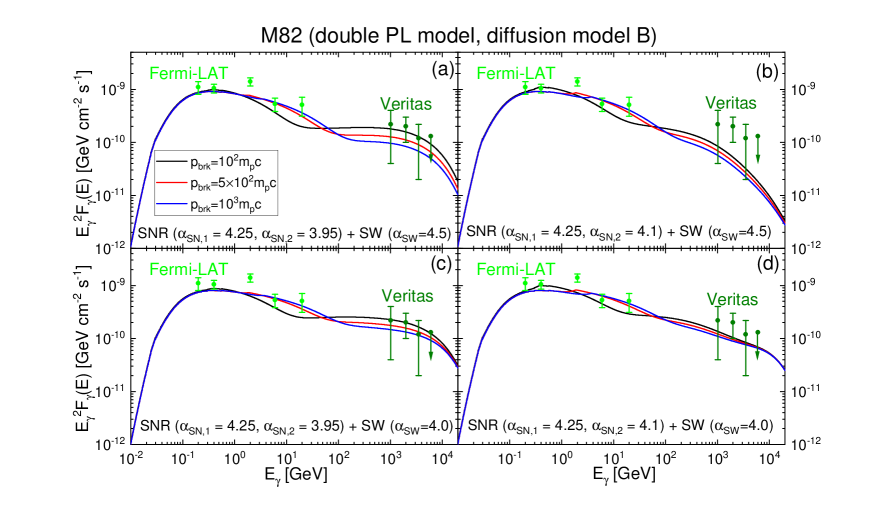
The $\gamma$-ray fluxes of M82 estimated with the double PL momentum distributions for SNR CRPs are shown in Figure 5 (with the diffusion model A) and Figure 6 (with the diffusion model B). The single PL momentum distributions with $\alpha_{\rm SW}=4.0$ or 4.5 are employed for SW CRPs. The predicted flux $F_{\gamma}$ in the energy range of $E_{\gamma}\lesssim 100$ GeV is insensitive to the diffusion model, since the transport of CRPs with $p\lesssim 1$ TeV/$c$ is controlled by the SBN wind advection. Hence, the Fermi-LAT data are reproduced for both of the diffusion models, if the slope of the low momentum part is adjusted, i.e., $\alpha_{\rm SN,1}=4.25$. On the other hand, $F_{\gamma}$ in the higher energy range is affected substantially by the diffusion model, because the transport time-scale of CRPs with $p\gtrsim 1$ TeV/$c$ is much longer in the diffusion model A than in the diffusion model B, as shown in Figure 3. The reproduction of the Veritas data for $E_{\gamma}\gtrsim 1$ TeV requires a softer spectrum in the high momentum part, e.g., $\alpha_{\rm SN,2}=4.1$ (see Fig. 5(b)), in the case of the diffusion model A, while it requires a harder spectrum, e.g., $\alpha_{\rm SN,2}=3.95$ (see Fig. 6(c)), in the case of the diffusion model B. Other model parameters involved are less important. Yet, somewhat better fittings are obtained with larger $\alpha_{\rm SW}$, such as 4.5, if the diffusion model A is adopted, and with smaller $\alpha_{\rm SW}$, such as 4.0, if the diffusion model B is adopted. The break momentum $p_{\rm brk}$ affects the predicted fluxes at high energies, but with the adopted range of $p_{\rm brk}\simeq 10^{2}-10^{3}m_{p}c$, the difference in $F_{\gamma}$ is at most a factor of two.

Figure 7 shows the $\gamma$-ray fluxes of NGC253 and Arp220 estimated with the double PL distributions for SNR CRPs. For $\alpha_{\rm SN,1}$, the values that reproduce the Fermi-LAT data are used. Again, with the diffusion model A (blue lines), a softer distribution at the high momentum part with $\alpha_{\rm SN,2}=4.1$ reproduces the the H.E.S.S. and Veritas observations better, while with the diffusion model B (red lines), a harder distribution with $\alpha_{\rm SN,2}=3.95$ does better. The model parameters used are listed in the figure caption.

In general, at $E_{\gamma}\lesssim 100$ GeV, the $\gamma$-ray observations by Fermi-LAT are well reproduced, regardless of the CRP production and diffusion models, once the slope of the SNR-produced CRP distribution, $\alpha_{\rm SN}$ or $\alpha_{\rm SN,1}$, is properly chosen. At $E_{\gamma}\gtrsim 1$ TeV, on the other hand, the results depend rather sensitively on both the CRP production and diffusion models. To examine the goodness of the fit to the $\gamma$-ray observations by Fermi-LAT, Veritas and H.E.S.S., we perform the $\chi^{2}$-test for M82 and NGC253 with enough data points, by calculating $\chi^{2}\equiv\sum[(F_{\rm\gamma,obs}-F_{\gamma})/F_{\rm\gamma,err}]^{2}$, where $F_{\gamma}$ is our estimated $\gamma$-ray flux, $F_{\rm\gamma,obs}$ and $F_{\rm\gamma,err}$ are the observed $\gamma$-ray flux and error, respectively; only the data points with error bar are used, while those of upper limit are excluded. The $\chi^{2}$-values and $p$-values for different combinations of the CRP production and diffusion models with the best fit parameters are given in Table 2. For both M82 and NGC253, the combination of the single PL model and the diffusion model A and the combination of the double PL model and the diffusion model B give better statistics. However, other combinations also have, for instance, the $p$-value within the 1 $\sigma$ level, and hence should not be statistically excluded. On the other hand, the number of observation data points, especially that for M82, seems to too small to differentiate different models. Our results imply that further $\gamma$-ray observations would be necessary to meaningfully constrain the CRP production and transport models in SBGs.

We then predict the neutrino fluxes from three nearby SBGs for three different combinations of CRP production and transport models with the best fit model parameters listed in Table 3. The combination of the single PL model for SNR CRPs and the diffusion model B is not included, since it shows the largest deviation from observation data. We again employ the formulae presented in Kelner et al. (2006). The neutrino source function as a function of neutrino energy $E_{\nu}$ is given as

where $x=E_{\nu}/E_{\pi}$. The term $f_{\nu_{\mu}^{(1)}}(x)$ represents the muon neutrino production through the pion decay $\pi\rightarrow\mu\nu_{\mu}$, and $f_{\nu_{\mu}^{(2)}}(x)$ and $f_{\nu_{e}}(x)$ describe the muon and electron neutrino productions through the muon decay $\mu\rightarrow\nu_{\mu}\nu_{e}e$. The formulae for $f_{\nu_{\mu}^{(1)}}$, $f_{\nu_{\mu}^{(2)}}$, and $f_{\nu_{e}}$ are given in Kelner et al. (2006). Then, the neutrino flux observed at the Earth is calculated as

Figure 8 shows the predicted neutrino fluxes, $F_{\nu}$, for two values of the maximum momentum of CRP distributions, $p_{\rm max}=100~{}{\rm PeV}/c$ (upper panels) and $p_{\rm max}=1~{}{\rm PeV}/c$ (lower panels). We compare $F_{\nu}$ to the point source sensitivity ranges of IceCube, IceCube-Gen2, and KM3NET: $E_{\nu}^{2}F_{\nu}\sim 5\times 10^{-10}-10^{-8}~{}{\rm GeV~{}cm^{-2}s^{-1}}$ in the energy range of $E_{\nu}\gtrsim 60$ TeV for IceCube with seven-year data (Aartsen et al., 2017), $E_{\nu}^{2}F_{\nu}\sim 5\times(10^{-11}-10^{-10})~{}{\rm GeV~{}cm^{-2}s^{-1}}$ in the energy range of $E_{\nu}\gtrsim 60$ TeV for IceCube-Gen2 with fifthteen-year data (van Santen & IceCube-Gen2 Collaboration, 2017), and $E_{\nu}^{2}F_{\nu}\sim(2-4)\times 10^{-10}~{}{\rm GeV~{}cm^{-2}s^{-1}}$ in the energy range of $E_{\nu}\sim 15$ TeV $-$ 1 PeV expected for KM3NET with six-year data (Aiello et al., 2019). The point source sensitivity in the figure is defined as the median upper limit at the 90% confidence level. We also compare $F_{\nu}$ to the atmospheric muon and electron neutrino fluxes (Richard et al., 2016). A circular beam of $1^{\circ}$ diameter is used for the calculation of the fluxes shown in the figure.

With the adopted range of $p_{\rm max}\simeq 1-100$ PeV/$c$, the $\gamma$-ray fluxes presented in the previous section are insensitive to $p_{\rm max}$, due to the exponential attenuation included in Equation (14). However, $F_{\nu}(E_{\nu})$ for high energy neutrinos exhibits strong dependence on the assumed value of $p_{\rm max}$. With larger $p_{\rm max}$, $F_{\nu}$ extends to higher energies. But the amount of highest energy neutrinos is determined not just by $p_{\rm max}$, but also by the diffusion model. If the diffusion time-scale of CRPs is shorter at high energies, $F_{\nu}$ should be lower. Hence, $F_{\nu}$ is smaller at highest energies with the diffusion model B than with the diffusion model A in Figure 8. As mentioned in Section 3, in the diffusion model B, the streaming speed of CRPs approaches the speed of light at $p\gtrsim 0.1$ PeV/$c$; that is, the streaming speed may be overestimated and the diffusion time-scale may be underestimated, and then $F_{\nu}$ may be underestimated at highest energies. Yet, in all the models considered in Figure 8, which fit $\gamma$-ray observations reasonably well, the predicted $F_{\nu}$ at $E_{\nu}\gtrsim 0.1$ PeV from nearby SBGs is at least an order of magnitude smaller than the lower bound of the point source sensitivity of IceCube. Thus, SBGs may not be observed as point sources in IceCube. SBGs could be still a major contributor of diffuse high-energy neutrinos, as pointed in previous works (see the introduction for references), but the amount of estimated contributions should depend on the details of modeling including the diffusion model.

Our results suggest that nearby SBGs, especially M82 and also NGC253, might be observed as point sources in the range of 15 TeV $\lesssim E_{\nu}\lesssim 1$ PeV with KM3NET and also in the range of 60 TeV $\lesssim E_{\nu}\lesssim 10$ PeV with IceCube-Gen2, in the most optimistic cases with the diffusion model A and $p_{\rm max}=100$ PeV/$c$, shown in panels (a) and (b) of Figure 8. On the other hand, other models predict $F_{\nu}$ that does not touch the point source sensitivities boxes of KM3NET and IceCube-Gen2, indicating that nearby SBGs would be difficult to be detected as point sources. We point that the observations of neutrinos from nearby SBGs would help constrain the CRP production and transport models there.

At lower energies of $E_{\nu}\lesssim 1$ TeV, the neutrino flux has been obtained, for instance, in Super-Kamiokande (e.g., Hagiwara et al., 2019). However, $F_{\nu}$ from nearby SBGs is predicted to be orders of magnitude smaller than the atmospheric muon neutrino flux. So it would not be easy to separate the signature of neutrinos from SBGs in the data of ground facilities such as Super-Kamiokande and future Hyper-Kamiokande (e.g., Abe et al., 2011).

We have estimated the CRP production by SWs from massive stars and SNRs from core-collapse SNe inside the SBN of nearby SBGs. Considering the lack of full understanding of nonlinear interrelationships among complex kinetic processes involved in the DSA theory, we have adopted both the canonical single PL model with $\alpha_{\rm SN}$ and the double PL model with $\alpha_{\rm SN,1}$ and $\alpha_{\rm SN,2}$ for the SNR-produced CRP momentum distribution. The latter is intended to represent a concave spectrum that might arise due to nonlinear dynamical feedback from the CR pressure, if $\sim 10$ % of the shock kinetic energy is transferred to CRPs. For the SW-produced CRP distribution, only the single PL model with $\alpha_{\rm SW}$ is considered.

For the transport of CRPs inside the SBN, we have adopted two different diffusion models; CRPs scatter off either the large-scale turbulence of $\delta B_{\rm SBN}/B_{\rm SBN}\sim 1$ present in the SBN (diffusion model A) or the waves self-excited by CR streaming instability (diffusion model B) (Peretti et al., 2019; Krumholz et al., 2020). The diffusion model B assumes that the pre-existing turbulence of scales less than the gyroradius of CRPs with $E_{\rm CR}\lesssim{\rm several}\times 0.1~{}{\rm PeV}$ damps out by ion-neutral collisions.

Using the CRP momentum spectrum given in Equation (8) and the analytic approximations for source functions presented by Kelner et al. (2006), we have then calculated the $\gamma$-ray and neutrino emissions due to $pp$ collisions in the SBN, and estimated their fluxes from three nearby SBGs, M82, NGC253, and Arp220, observable at the Earth.

Main findings are summarized as follows.

(1) If the single PL model for SNR-produced CRPs is adopted, the $\gamma$-ray observations of Fermi-LAT, Veritas, and H.E.S.S. are better reproduced with the diffusion model A than with the model B. If the double PL model is adopted, on the other hand, the observations seem to be better reproduced with the diffusion model B. However, other combinations, although statistically somewhat less significant, cannot be excluded.

(2) The contribution of SW-produced CRPs may depend on the IGIMF; SBGs with higher SFRs are likely to have flatter IGIMFs, resulting in larger ratios of $\mathcal{L}_{\rm SW}/\mathcal{L}_{\rm SN}$. In Arp220 where the star formation rate is high, the SW-produced CRPs may make a significant contribution to the $\gamma$-ray emission.

(3) The predicted neutrino fluxes from three nearby SBGs seem too small, so that SBGs would not be observed as point sources by IceCube. On the other hand, our estimation suggests that M82 and NGC253 might be detectable as point sources with the upcoming KM3NeT and IceCube-Gen2, if the diffusion model A along with $p_{\rm max}=100$ PeV/$c$ is employed. In other models, the predicted neutrino fluxes would not be high enough to be detected as point sources by KM3NeT or IceCube-Gen2.

(4) Considering uncertainties in the CRP production and transport models in the SBN, we have examined various combinations of models in this paper. Based on our results, we point that currently available $\gamma$-ray observations may not provide sufficient information to differentiate the CRP production and transport models. However, those models could be further constrained with “multi-messenger observations” including possible detections of neutrinos from SBGs with future neutrino telescopes, such as KM3NET and IceCube-Gen 2, as well as further TeV-range $\gamma$-rays observations.

Finally, Müller et al. (2020) recently suggested that high-energy processes associated with superwinds driven by the supersonic outflows from the SBN (not stellar winds) can produce CRPs as well. But their contribution to $\gamma$-ray emissions from SBGs would be $\lesssim 10\%$, so that the main results of this paper would not be changed even when such contribution is included.

References

- Aartsen et al. (2017) Aartsen, M. G., Abraham, K., Ackermann, M., et al. 2017, ApJ, 835, 151, doi: 10.3847/1538-4357/835/2/151
- Abdo et al. (2010) Abdo, A. A., Ackermann, M., Ajello, M., et al. 2010, ApJ, 709, L152, doi: 10.1088/2041-8205/709/2/L152
- Abdollahi et al. (2020) Abdollahi, S., Acero, F., Ackermann, M., et al. 2020, ApJS, 247, 33, doi: 10.3847/1538-4365/ab6bcb
- Abe et al. (2011) Abe, K., Abe, T., Aihara, H., et al. 2011, arXiv e-prints, arXiv:1109.3262. https://arxiv.org/abs/1109.3262
- Abramowski et al. (2012) Abramowski, A., Acero, F., Aharonian, F., et al. 2012, ApJ, 757, 158, doi: 10.1088/0004-637X/757/2/158
- Acero et al. (2009) Acero, F., Aharonian, F., Akhperjanian, A. G., et al. 2009, Science, 326, 1080, doi: 10.1126/science.1178826
- Acero et al. (2015) Acero, F., Ackermann, M., Ajello, M., et al. 2015, ApJS, 218, 23, doi: 10.1088/0067-0049/218/2/23
- Aiello et al. (2019) Aiello, S., Akrame, S. E., Ameli, F., et al. 2019, Astroparticle Physics, 111, 100, doi: 10.1016/j.astropartphys.2019.04.002
- Ajello et al. (2020) Ajello, M., Di Mauro, M., Paliya, V. S., & Garrappa, S. 2020, ApJ, 894, 88, doi: 10.3847/1538-4357/ab86a6
- Balogh & Treumann (2013) Balogh, A., & Treumann, R. A. 2013, Physics of Collisionless Shocks, Vol. 12, doi: 10.1007/978-1-4614-6099-2
- Bechtol et al. (2017) Bechtol, K., Ahlers, M., Di Mauro, M., Ajello, M., & Vandenbroucke, J. 2017, ApJ, 836, 47, doi: 10.3847/1538-4357/836/1/47
- Bell (1978) Bell, A. R. 1978, MNRAS, 182, 147, doi: 10.1093/mnras/182.2.147
- Berezhko & Ellison (1999) Berezhko, E. G., & Ellison, D. C. 1999, ApJ, 526, 385, doi: 10.1086/307993
- Berezhko & Völk (2000) Berezhko, E. G., & Völk, H. J. 2000, A&A, 357, 283. https://arxiv.org/abs/astro-ph/0002411
- Bykov (2014) Bykov, A. M. 2014, A&A Rev., 22, 77, doi: 10.1007/s00159-014-0077-8
- Bykov et al. (2014) Bykov, A. M., Ellison, D. C., Osipov, S. M., & Vladimirov, A. E. 2014, ApJ, 789, 137, doi: 10.1088/0004-637X/789/2/137
- Bykov et al. (2020) Bykov, A. M., Marcowith, A., Amato, E., et al. 2020, Space Sci. Rev., 216, 42, doi: 10.1007/s11214-020-00663-0
- Caprioli et al. (2010) Caprioli, D., Amato, E., & Blasi, P. 2010, Astroparticle Physics, 33, 160, doi: 10.1016/j.astropartphys.2010.01.002
- Caprioli et al. (2009) Caprioli, D., Blasi, P., Amato, E., & Vietri, M. 2009, MNRAS, 395, 895, doi: 10.1111/j.1365-2966.2009.14570.x
- Caprioli et al. (2020) Caprioli, D., Haggerty, C. C., & Blasi, P. 2020, arXiv e-prints, arXiv:2009.00007. https://arxiv.org/abs/2009.00007
- Caprioli & Spitkovsky (2014) Caprioli, D., & Spitkovsky, A. 2014, ApJ, 783, 91, doi: 10.1088/0004-637X/783/2/91
- Casse & Paul (1980) Casse, M., & Paul, J. A. 1980, ApJ, 237, 236, doi: 10.1086/157863
- Cesarsky & Montmerle (1983) Cesarsky, C. J., & Montmerle, T. 1983, Space Sci. Rev., 36, 173, doi: 10.1007/BF00167503
- Dabringhausen et al. (2012) Dabringhausen, J., Kroupa, P., Pflamm-Altenburg, J., & Mieske, S. 2012, ApJ, 747, 72, doi: 10.1088/0004-637X/747/1/72
- Drury (1983) Drury, L. O. 1983, Reports on Progress in Physics, 46, 973, doi: 10.1088/0034-4885/46/8/002
- Ekström et al. (2012) Ekström, S., Georgy, C., Eggenberger, P., et al. 2012, A&A, 537, A146, doi: 10.1051/0004-6361/201117751
- Franceschini & Rodighiero (2017) Franceschini, A., & Rodighiero, G. 2017, A&A, 603, A34, doi: 10.1051/0004-6361/201629684
- Freyer et al. (2003) Freyer, T., Hensler, G., & Yorke, H. W. 2003, ApJ, 594, 888, doi: 10.1086/376937
- Fryer et al. (2012) Fryer, C. L., Belczynski, K., Wiktorowicz, G., et al. 2012, ApJ, 749, 91, doi: 10.1088/0004-637X/749/1/91
- Georgy et al. (2013) Georgy, C., Walder, R., Folini, D., et al. 2013, A&A, 559, A69, doi: 10.1051/0004-6361/201321226
- H. E. S. S. Collaboration et al. (2018) H. E. S. S. Collaboration, Abdalla, H., Aharonian, F., et al. 2018, A&A, 617, A73, doi: 10.1051/0004-6361/201833202
- Hagiwara et al. (2019) Hagiwara, K., Abe, K., Bronner, C., et al. 2019, ApJ, 887, L6, doi: 10.3847/2041-8213/ab5863
- Janka (2012) Janka, H.-T. 2012, Annual Review of Nuclear and Particle Science, 62, 407, doi: 10.1146/annurev-nucl-102711-094901
- Kang (2012) Kang, H. 2012, Journal of Korean Astronomical Society, 45, 127, doi: 10.5303/JKAS.2012.45.5.127
- Kang (2013) —. 2013, Journal of Korean Astronomical Society, 46, 49, doi: 10.5303/JKAS.2013.46.1.049
- Kang & Jones (2007) Kang, H., & Jones, T. W. 2007, Astroparticle Physics, 28, 232, doi: 10.1016/j.astropartphys.2007.05.007
- Kang & Ryu (2010) Kang, H., & Ryu, D. 2010, ApJ, 721, 886, doi: 10.1088/0004-637X/721/1/886
- Kang & Ryu (2018) —. 2018, ApJ, 856, 33, doi: 10.3847/1538-4357/aab1f2
- Kelner et al. (2006) Kelner, S. R., Aharonian, F. A., & Bugayov, V. V. 2006, Phys. Rev. D, 74, 034018, doi: 10.1103/PhysRevD.74.034018
- Kennicutt & Evans (2012) Kennicutt, R. C., & Evans, N. J. 2012, ARA&A, 50, 531, doi: 10.1146/annurev-astro-081811-125610
- Krumholz et al. (2020) Krumholz, M. R., Crocker, R. M., Xu, S., et al. 2020, MNRAS, 493, 2817, doi: 10.1093/mnras/staa493
- Loeb & Waxman (2006) Loeb, A., & Waxman, E. 2006, J. Cosmology Astropart. Phys, 2006, 003, doi: 10.1088/1475-7516/2006/05/003
- Marcowith et al. (2016) Marcowith, A., Bret, A., Bykov, A., et al. 2016, Reports on Progress in Physics, 79, 046901, doi: 10.1088/0034-4885/79/4/046901
- Müller et al. (2020) Müller, A. L., Romero, G. E., & Roth, M. 2020, MNRAS, 496, 2474, doi: 10.1093/mnras/staa1720
- Murase et al. (2013) Murase, K., Ahlers, M., & Lacki, B. C. 2013, Phys. Rev. D, 88, 121301, doi: 10.1103/PhysRevD.88.121301
- Palla et al. (2020) Palla, M., Calura, F., Matteucci, F., et al. 2020, MNRAS, 494, 2355, doi: 10.1093/mnras/staa848
- Peng et al. (2016) Peng, F.-K., Wang, X.-Y., Liu, R.-Y., Tang, Q.-W., & Wang, J.-F. 2016, ApJ, 821, L20, doi: 10.3847/2041-8205/821/2/L20
- Peretti et al. (2019) Peretti, E., Blasi, P., Aharonian, F., & Morlino, G. 2019, MNRAS, 487, 168, doi: 10.1093/mnras/stz1161
- Peretti et al. (2020) Peretti, E., Blasi, P., Aharonian, F., Morlino, G., & Cristofari, P. 2020, MNRAS, 493, 5880, doi: 10.1093/mnras/staa698
- Ptuskin & Zirakashvili (2005) Ptuskin, V. S., & Zirakashvili, V. N. 2005, A&A, 429, 755, doi: 10.1051/0004-6361:20041517
- Richard et al. (2016) Richard, E., Okumura, K., Abe, K., et al. 2016, Phys. Rev. D, 94, 052001, doi: 10.1103/PhysRevD.94.052001
- Romero et al. (2018) Romero, G. E., Müller, A. L., & Roth, M. 2018, A&A, 616, A57, doi: 10.1051/0004-6361/201832666
- Salpeter (1955) Salpeter, E. E. 1955, ApJ, 121, 161, doi: 10.1086/145971
- Seo et al. (2018) Seo, J., Kang, H., & Ryu, D. 2018, Journal of Korean Astronomical Society, 51, 37, doi: 10.5303/JKAS.2018.51.2.37
- Sudoh et al. (2018) Sudoh, T., Totani, T., & Kawanaka, N. 2018, PASJ, 70, 49, doi: 10.1093/pasj/psy039
- Tamborra et al. (2014) Tamborra, I., Ando, S., & Murase, K. 2014, J. Cosmology Astropart. Phys, 2014, 043, doi: 10.1088/1475-7516/2014/09/043
- Tatischeff (2009) Tatischeff, V. 2009, A&A, 499, 191, doi: 10.1051/0004-6361/200811511
- The VERITAS Collaboration et al. (2015) The VERITAS Collaboration, Abeysekara, A. U., Archambault, S., et al. 2015, arXiv e-prints, arXiv:1510.01639. https://arxiv.org/abs/1510.01639
- van Santen & IceCube-Gen2 Collaboration (2017) van Santen, J., & IceCube-Gen2 Collaboration. 2017, in International Cosmic Ray Conference, Vol. 301, 35th International Cosmic Ray Conference (ICRC2017), 991
- VERITAS Collaboration et al. (2009) VERITAS Collaboration, Acciari, V. A., Aliu, E., et al. 2009, Nature, 462, 770, doi: 10.1038/nature08557
- Vladimirov et al. (2008) Vladimirov, A. E., Bykov, A. M., & Ellison, D. C. 2008, ApJ, 688, 1084, doi: 10.1086/592240
- Wang & Fields (2018) Wang, X., & Fields, B. D. 2018, MNRAS, 474, 4073, doi: 10.1093/mnras/stx2917
- Weaver et al. (1977) Weaver, R., McCray, R., Castor, J., Shapiro, P., & Moore, R. 1977, ApJ, 218, 377, doi: 10.1086/155692
- Weidner et al. (2013) Weidner, C., Kroupa, P., Pflamm-Altenburg, J., & Vazdekis, A. 2013, MNRAS, 436, 3309, doi: 10.1093/mnras/stt1806
- Yan et al. (2017) Yan, Z., Jerabkova, T., & Kroupa, P. 2017, A&A, 607, A126, doi: 10.1051/0004-6361/201730987
- Yang et al. (2016) Yang, R., Aharonian, F., & Evoli, C. 2016, Phys. Rev. D, 93, 123007, doi: 10.1103/PhysRevD.93.123007
- Zirakashvili & Ptuskin (2012) Zirakashvili, V. N., & Ptuskin, V. S. 2012, Astroparticle Physics, 39, 12, doi: 10.1016/j.astropartphys.2011.09.003
- Zirakashvili & Ptuskin (2016) —. 2016, Astroparticle Physics, 78, 28, doi: 10.1016/j.astropartphys.2016.02.004
- Zirakashvili & Ptuskin (2018) —. 2018, Astroparticle Physics, 98, 21, doi: 10.1016/j.astropartphys.2018.01.005