Modeling of the contrast-enhanced perfusion test in liver based on the multi-compartment flow in porous media
Abstract
The paper deals with modeling the liver perfusion intended to improve quantitative analysis of the tissue scans provided by the contrast-enhanced computed tomography (CT). For this purpose, we developed a model of dynamic transport of the contrast fluid through the hierarchies of the perfusion trees. Conceptually, computed time-space distributions of the so-called tissue density can be compared with the measured data obtained from CT; such a modeling feedback can be used for model parameter identification. The blood flow is characterized at several scales for which different models are used. Flows in upper hierarchies represented by larger branching vessels are described using simple 1D models based on the Bernoulli equation extended by correction terms to respect the local pressure losses. To describe flows in smaller vessels and in the tissue parenchyma, we propose a 3D continuum model of porous medium defined in terms of hierarchically matched compartments characterized by hydraulic permeabilities. The 1D models corresponding to the portal and hepatic veins are coupled with the 3D model through point sources, or sinks. The contrast fluid saturation is governed by transport equations adapted for the 1D and 3D flow models. The complex perfusion model has been implemented using the finite element and finite volume methods. We report numerical examples computed for anatomically relevant geometries of the liver organ and of the principal vascular trees. The simulated tissue density corresponding to the CT examination output reflects a pathology modeled as a localized permeability deficiency.
Keywords: Liver perfusion Porous media Darcy flowBernoulli equationTransport equation Dynamic contrast-enhanced computed tomography
1 Introduction
Modeling blood perfusion in tissues belongs to the most challenging problems in the biomechanical and biomedical research. The topic is of interest especially in liver surgery (Plantefèv et al, 2016), brain neurosurgery, or neurology (Dai et al, 2016; Reichold et al, 2009; Reichold, 2011). Although the functionality of the two related organs, liver and brain, is completely different, there are some similar aspects for both. In contrast with the myocardium, another highly perfused tissue, for both the organs the phenomenon of deformation can be neglected unless special concerns are in focus, see e.g. Peterlik et al (2012). It is desirable to find accurately parts of the tissue with an insufficient blood supply, to localize anomalies in the blood microcirculation, and to quantify locally the perfusion efficiency. It is worth to note that also the kidney belongs to highly perfused tissues with its important role in the blood circulation system, but we do not tackle this issue in the present paper.
In most perfused organs, the blood is transported through complex hierarchical branching systems of vessels with various diameters which diminish consecutively at each bifurcation, beginning from arteries down to capillaries. The ascending system of veins is arranged in the reversed sense, starting at the capillary level, where the blood participates in the metabolism process, delivering the oxygen to the tissue and collecting the waste products. The blood circulation in the tissue can be represented by two penetrating, but mutually separated vascular trees connected only at the capillary level. In reality, collateralization vessels exist which make shunts between the two trees, but this phenomenon is usually negligible for the global hierarchically built system.
Although the modeling approach is presented in a rather general setting, in this paper, we focus on the liver tissue which has a special structure. The blood flows in the whole organ from two separated vascular trees, one connected to the hepatic artery (HA) and the other to the portal vein (PV), whereby the venous supply dominates. The two branching systems bifurcate to about 20 generations (Debbaut et al, 2014). The blood is filtered in the tissue functional units, called hepatic units, or lobules, which typically are considered as hexagonal prisms. At their corner edges, the hepatic artery and portal vein trees terminate and the blood flows through hepatic capillaries constituting the sinusoids to the so-called central veins, the terminal branches of the draining hepatic vein (HV) located in the center of each lobule. In the proposed model, for simplicity we neglect the HA, as its blood supply is minor in the comparison with the one by the portal vein111The perfusion model is intended to estimate the volume regeneration capacity of the liver parenchyma (Brůha et al, 2015). In this context, it is important to capture the supply through the portal vein. Concerning the perfusion CT simulation, we focus on the second stage when the contrast bolus arrives at the PV inlet so that the first stage associated with the HA is over..
The steadily growing body of published works related to the modeling of liver perfusion shows its importance for the medical research. Obviously, relevant computational models which can be used for complex simulations involving various parameters require detailed information about the liver structure. However, there is a pertaining difficulty in describing the vascular trees bridging several scales. The current standard computed tomography (CT), magnetic resonance imaging (MRI) and related image processing techniques provide resolution of the vascular trees down to millimeters, which is not enough to capture details on about 10 underlying tree generations. Therefore, various methods and algorithms have been proposed to generate artificial, but anatomically correct vascular architectures. These are coupled with the authentic patient-specific reconstructed geometry to obtain complete vascular trees with a required resolution of microvessels. The most popular approach is based on the constrained constructive optimization (CCO), see e.g. Georg et al (2010), Schwen and Preusser (2012). However, there are more advanced approaches based on the metabolism driven processes of the vascular tree reconstruction (Schneider et al, 2012).
Rather than modeling the flow on the complex branching system, many publications have been devoted to detailed studies of microcirclation. Perfusion characteristics of blood flow through hepatic microcapillaries of human lobular sinusoids were analyzed by Debbaut et al (2012) using tissue samples processed by corrosion casting and the micro-CT imaging; anisotropic tensors of the sinusoidal permeability were calculated by a simple averaging of the flow field obtained using standard CFD simulations. Blood circulation in the liver lobule was considered in Bonfiglio et al (2010) using both Newtonian and shear-thinning flow models. The liver tissue is able to adapt rapidly to modified hydraulic conditions; in Ricken et al (2010), the sinusoidal permeability has been studied in terms of a vascular remodeling process induced by outflow obstruction. Sinusoidal vascular canals were assumed to align with the blood pressure gradient. In Ricken et al (2015), using the general framework of a two-scale approach and the theory of porous media, the basic coupled transport-reaction mechanisms between blood perfusion and the hepatic cell metabolism were described at the level of lobule. Lymphatic flow production in the liver lobules arranged in periodic lattices was treated in Siggers et al (2014). A similar approach has been used in Lettmann and Hardtke-Wolenski (2014) to study microcirculation driven transport of oxygen and cytokine in the tissue. Besides the blood flow in healthy liver itself, diseased tissue deserve attention from medical point of view, but also as a challenge for mathematical modeling; there is a considerable number of issues related to modeling pathophysiological conditions, such as the fluid transport through vascular tumors (Pozrikidis, 2010; Shipley and Chapman, 2010; Mescam et al, 2010).
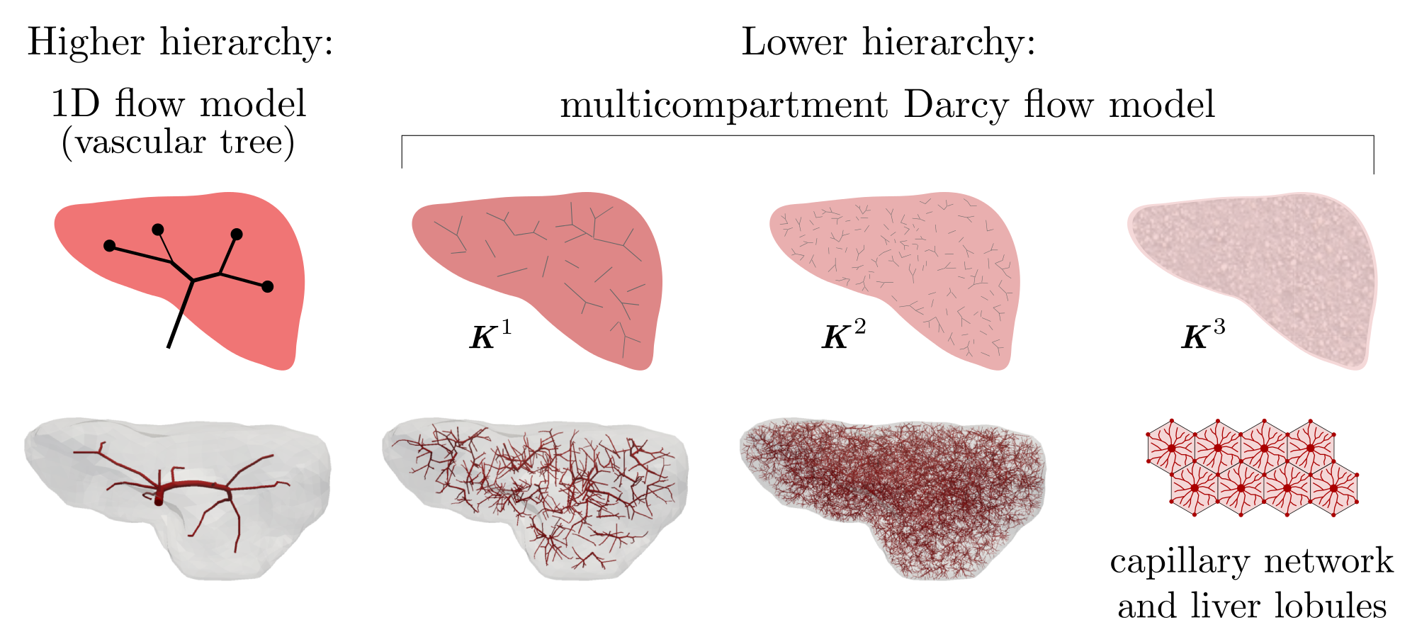
Since the straightforward mathematical description of blood flow on the complete vascular trees featured by several hierarchies using the Navier-Stokes equations leads to a prohibitively complicated numerical model, some convenient model reduction is needed. We adhere to the general approach proposed in Formaggia et al (2009) which consists in decomposing the tree into a higher (HH) and a lower (LH) hierarchy, see Fig. 1.
The HH tree is constituted by larger vessels, so that the flow can be described in the 3D geometry using the Navier-Stokes equations. Alternatively the vessels can be replaced with line segments, so that the flow model is obtained using the 1D description of flow on such branching system of line segments.
To describe the blood flow in the LH tree, we resort to a type of the Darcy flow model which is defined in the 3D bulk of the liver parenchyma. Since the LH part involves vessels associated with different hierarchies, several compartments are introduced and Darcy model is used within each of them. The flow between different compartments is described in terms of the difference between the compartmental pressure at a given location; details are given below.
Remark
The multicompartment model of perfusion has been used e.g. in Cimrman and Rohan (2007) and then in Jonášová et al (2014) as a phenomenological model. Recently a multicompartment model of cardiac perfusion was presented in Michler et al (2013), cf. Hyde et al (2013). For two compartments it can be derived using the homogenization of the Darcy flow in porous medium with large contrasts in the permeability (Rohan and Cimrman, 2010; Rohan et al, 2012a). Another derivation is based on the averaging theory by Slattery and Whitaker (Slattery, 1967; Whitaker, 1967) employed to the hierarchical flow in pores with continuously variable cross-sections, cf. Huyghe and Campen (1995).
In the context of the multi-porous, media employed in the geophysical research, phenomenological approaches based on extensions of the Biot model (Mehrabian and Abousleiman, 2014) lead to multi-compartment models where co-existing porosities are associated with distinct pressures. As a special case, the double-porous, or double-permeability media was obtained by homogenization approach applied to upscale periodic structures with large contrasts in the hydraulic permeability (Rohan and Cimrman, 2010; Rohan et al, 2012b). The derived model describing fluid flow in the double-permeability medium with two systems of periodic channels separated by low permeable matrix can be adapted to the liver parenchyma generated as a quasi-periodic structure of lobules.
The aim of the present paper is twofold:
-
1.
we present a numerically tractable model of the liver perfusion intended for real-time simulations, which is based on the hierarchical decomposition of the perfusion trees, combining approaches of the multicompartment porous media flow and the “1D” flow on vascular trees;
-
2.
we propose an associated model of transport of the contrast agent dissolved in the blood and characterized by the saturation function.
The latter model provides an analogous output to the so-called tissue density (measured in the Hounsfield units) which is obtained from the medical perfusion examination by the dynamic contrast-enhanced CT, or alternatively by the magnetic resonance imaging, see e.g. Fieselmann et al (2011); Keeling et al (2007). We would like to stress out that this modeling option is important for the model parameters identification and, thereby, also for the model validation.
The conception of the hierarchical modeling reported in this paper has been outlined in a short proceedings paper (Jonášová et al, 2014). However, here we give additional details on the model itself and present new results computed for anatomically relevant data, including the anisotropic permeability coefficients estimated by an analysis of the perfusion trees.
The organization of the paper is as follows. The perfusion model based on the hierarchical decomposition of the perfusion trees (the portal and hepatic veins) is described in Section 2. In Section 3, the transport of the contrast fluid is introduced. In Section 4 we present numerical examples to illustrate an application of the model to describe the hierarchical blood flow in a “liver” which is a simplified geometrical structure created using anatomical data combined with the CCO approach to define the portal and hepatic vascular trees. The paper conclusions and the discussion of further perspectives is presented in Section 5.
2 Hierarchical mathematical model of perfusion
The simulation of blood perfusion in tissues, such as the hepatic or cerebral ones, belongs to problems typically requiring a sort of multiscale modeling approach (D’Angelo, 2007). The term “multiscale” is employed in a slightly different manner than in Formaggia et al (2009), where the “geometrical multiscale” modeling was introduced in the context of the cardiovascular system. The difficulty of blood perfusion modeling arises from the nature of the flow in the perfusion trees incorporating blood vessels of very different diameters. In liver, the blood is conveyed to the organ by the portal vein which has the diameter of about . The perfusion trees have several hierarchies associated with bifurcations, where vessel diameters reduce. The tissue parenchyma is arranged in hexagonal structures (lobules) with the characteristic size of 1.5 mm where the blood is transported through the capillaries with the diameter of about from the portal compartment to the hepatic one. Thus, the overall scale change characterized by the ratio of the largest and smallest diameters of the vascular trees is approximately .
The model which we develop should allow also for simulation of the transport of the contrast fluid (the tracer) during the contrast-enhanced dynamic perfusion test. The aim is to provide a computational feedback which would enable us to analyze more accurately the CT scans obtained from the standard dynamic perfusion test of a patient (Materne et al, 2000). The methods currently being used are based on the deconvolution, or maximum slope techniques. They provide some local integral characteristics like the blood flow, blood volume, mean transition times and others for each voxel of the tissue (Koh et al, 2006; Fieselmann et al, 2011). Our approach should provide an alternative and more detailed interpretation of the measured CT scans. The proposed strategy announced first in our conference paper (Jonášová et al, 2014) is based on the following tasks:
-
•
to describe flows in the perfusion trees including the parenchyma by combining suitable models which are associated with different hierarchies and which use the most information about the structures and geometry, involving only few undetermined parameters;
- •
-
•
to identify selected parameters of the perfusion model (like permeability), so that the simulated dynamic CT examination well approximates the measured data (Rohan et al, 2015a).
Such a “tuned” model would enable us to analyze the blood flow in particular compartments and to predict effects of intended medical treatment, like resection of a part of the tissue.
In the proposed strategy, several difficulties arise: on one hand, the model should reflect the microstructure and fit the complex geometry of the perfusion trees, on the other hand, it should be parametrized using just not too many parameters, to prevent ill conditioning of the “tuning” step involving simulations of the steady blood flow and the dynamic tracer transport. Therefore, the tuning parameters must reflect some important features of the perfusion system.
The model of the perfusion and of the contrast fluid transport described in this paper consists of the following two parts:
-
1.
The “inlet” and “outlet” trees which are associated with the portal and hepatic vein networks222We have in mind the liver perfusion modeling, so that we also adapt the notations to fit with this particular application. (in the case of the liver; recall that we have neglected the hepatic artery in the model). These trees are denoted by and (label stands for the portal vein system, whereas label stands for the hepatic vein system). They are formed by vessel segments and junctions representing the bifurcations. The steady flow on these trees is described by a 1D model which is introduced in Section 2.3, see also Jonášová et al (2014). The model is relevant for higher hierarchies of the vascular trees, down to a certain size of the vessels, so that the terminal branches333or leaves in the graph theory terminology of and may have diameters about 1 mm.
-
2.
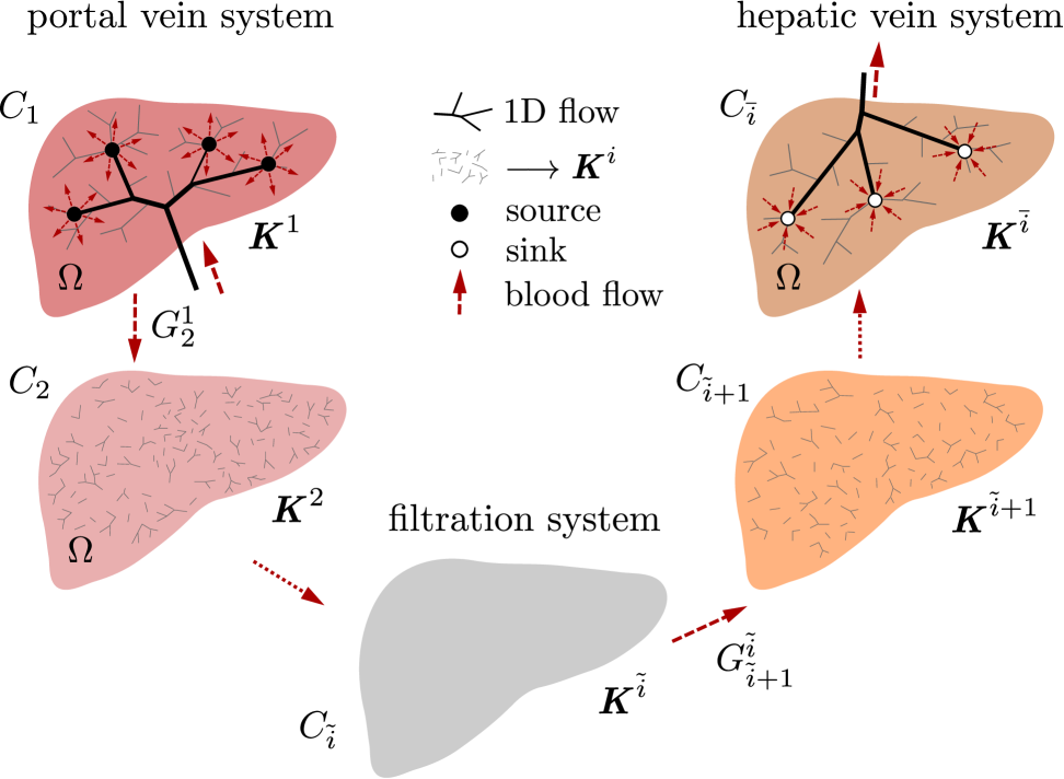
The tissue parenchyma including lower hierarchies of the “inlet” and “outlet” trees. The flow in this part of the vascular system is governed by the multi-compartment Darcy flow model in a porous medium. At any point of the liver occupying domain , several (at least two) different pressure values are defined which are associated with different compartments, see Section 2.2. There are point sources and sinks defined in , where the 1D trees are connected to the parenchyma model.
2.1 Structure of compartments
In this section we consider the lower hierarchies of the vascular trees. We consider a part of tissue (or the whole organ) occupying the domain . The compartments are established as continuum representations of the connected vascular network (or tree, as the special case) restricted by a given range of characteristic vessel cross-sections. Denoting by the total number of considered hierarchies, such a range is indicated by the hierarchy index , whereby hierarchies correspond to the precapillary vessels of the lobular structure. Denoting by the typical (or mean) vessel cross section in the given hierarchy, it holds that whenever . Each compartment is associated with the group; typically there are two groups labeled by index , corresponding to the portal and hepatic vein systems (should also the hepatic artery be included in the model, another group, say would be included). We shall identify compartments by a simple index given by the group and the hierarchy , whereby denotes the index set of all compartments. Any compartment is represented by a subdomain and by the hydraulic permeability tensor which can be introduced using an averaging procedure once the underlying tree segment (denoted by ) is known. This point will be discussed below in Section 4. For a given compartment belonging to a group , let is the hierarchy index. The fluid between two distinct compartments and can be exchanged only in the overlap domain , and only, if either a) they belong to the same group and their hierarchies are closed, , or b) if and . More general rules of flow between compartments are possible, but would not be physiological, or would describe special anomalies in the vasculature.
Groups, hierarchies and volume fractions
The concept of volume fractions is a very natural basis to relate the model parameters with structural features. Vessels of a given group and associated with hierarchy are distributed at point with volume fractions . In the context of the present model, by we describe the local volume fraction of blood vessels comprised in compartment . Since , obviously . Denoting by is the volume fraction of all parts of the parenchyma which are not blood vessels and, thus, not being included in any compartment, the partition of unity expressed in terms of volume fractions of all components reads in two possible ways:
| (1) | ||||
| (2) |
at any point . Note that all volume fractions must be non-negative.
2.2 Multicompartment model of Darcy flow
We approximate the flow in lower hierarchies of the arterial and venous trees, including perfusion at the level of tissue parenchyma, using a macroscopic model describing parallel flows in defined compartments. The model is based on some more fundamental principles related to homogenization, see Remark in Section 1, but can simply be justified by the phenomenological approach. Similar models have been used in other works (Showalter and Visarraga, 2004; Cimrman and Rohan, 2007; Hyde et al, 2013).
The model involves pressures , associated with each compartment . Any -th compartment occupying domain can be saturated from an external source (or drained by a sink); in general one may define the local source/sink flux which expresses an amount of fluid supplied, or drained out from the compartment to the upper perfusion tree branches, and . Alternatively, the pressure can be prescribed in a given subdomain which may represent junctions with upper hierarchies of the perfusion system treated by the 1D flow model on branching networks, see Section 2.3. In practice, can be formed by a number of “small” balls , thus , labeled by index associated with the -th junction. The mass conservation for compartment is expressed by the following equations (to be satisfied in ):
| (3) | ||||
| (4) | ||||
| (5) |
where is the Darcy velocity, is the local permeability tensor associated with vessels of the -th compartment and is the local perfusion coefficient coupling compartments , so that describes the amount of fluid transported from to (drainage flux; obviously ). As the boundary conditions for (3), we consider the non-penetration condition on the outer surface, and a prescribed pressure on ,
| (6) | ||||
| (7) |
The numerical model is obtained by the finite-element discretization of the weak formulation of problem (3)-(7). We shall need the following admissibility sets:
| (8) | |||
| (9) |
In our numerical tests we consider being given by point values in vertices of the finite element mesh. For some compartments, can vanish, so that .
The weak formulation of the problem
constituted by equations (3)-(5) and the boundary conditions (6)-(7) is, as follows: Find with , such that for all compartments ,
| (10) |
The summation in the second term takes only over nonvanishing .
All parameters and depend on the local volume fractions . In fact, for a given tree, see Fig. 5, both these parameters can be computed point-wise in using an averaging approach reported in Vankan et al (1997); Hyde et al (2013) which is based on the theoretical result describing hierarchical flows (Huyghe and Campen, 1995). Then the following properties can be guaranteed:
-
•
is positive semi-definite 2nd order tensor for .
-
•
Domain .
-
•
for in the overlap subdomains .
Usually, when the averaging control volume is large enough w.r.t. the characteristic size of the vessel segments, is positive definite, however, if only one or two vessels are encountered in , is singular. For the numerical treatment, a regularization can be considered, e.g. using modified permeabilities , where , , but can be any relevant permeability value in domain , and is a small number.
Well posedness of the perfusion problem.
Assume nonvanishing Lipschitz open bounded domains , such that for each there exists a nonempty overlap domain and in . If at least for one compartment the Dirichlet boundary is nonempty, then the regularized problem (10), where is replaced by , yields a unique solution .
2.3 Flow on upper-level vascular trees
As announced above, the upper-level vascular trees, the arterial, or the venous one, should be treated by taking into account the specific geometry of the vessels. In order to obtain an efficient numerical model it has been suggested to consider a simplified flow model based on the Bernoulli equation. Thus, instead of the full CFD analysis of flow in complicated 3D vessel geometries, the perfusion tree is replaced by a system of line segments characterized by the length, the cross-section and a loss parameter which is related to the specific geometry of the vessel segment. To respect the tortuosity of the vascular network, the lengths associated with the line segments should correspond to the actual vessel length.
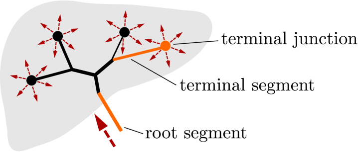
We consider a vascular tree constituted by vessel segments and junctions labeled by , see Fig. 3. Any is defined by its spatial position and by the connectivity set containing indices of segments connected at the junction. Although it is assumed that may form a graph with loops, in our study we consider only branching trees, so that is typically a bifurcation. The root and terminal junctions are just one-element sets. The number of all terminal junctions is denoted by . By we denote the root junction, whereas the terminal branches end by junctions through which they are connected with the continuum model described above in Section 2.2.
The simplest possible model of flow on is based on the Bernoulli equation. The flow in a tree is described by nodal pressures and segment velocities . In order to take into account the dissipation of the viscous flow, the pressure loss terms must be introduced by virtue of the Reynolds number associated with the flow on one segment. For any line segment featured by a “true” vessel length and its diameter which is assumed to be constant along the whole segment, the pressure drop related to the node pressures at the vessel end-points is related to the velocity by the following relationship
where is the blood density and is derived using the Poiseuille flow model; note that the Reynolds number depends on the velocity .
The flow model for the tree is assembled using the mass conservation (the continuity equation) expressed for each junction ,
| (11) |
where is the cross-section, and by the modified Bernoulli equation written for all branches of any bifurcations ,
| (12) |
where is the segment index of vessel connecting nodes and , i.e. , whereas is the source vessel of node . The final system of equations involving all bifurcations is solved by the Newton method.
2.4 Coupling the 1D and the multicompartment Darcy flow models
The 1D model is coupled with the model introduced in Section 2.2 through the terminal junctions which specify the sources and sinks for all the considered compartments of the upper-most hierarchy, i.e. for or . For the -th compartment saturated by the tree we define
| (13) | ||||
| (14) |
where is the Dirac distribution centered at point which is associated with the terminal junction of the 1D model. The pressures at these junctions represented by are coupled with the pressure fields in parenchyma, as expressed by condition (14). In practice, we use an approximation of which is based upon the specific finite element discretization, and (14) is replaced by so that only nodal value of the pressure is shared.
We conclude by a simple iterative algorithm used to compute the perfusion pressure and velocity fields in a steady state which is reached by increments for a pseudo-time step. Since there are two trees , as illustrated in Fig. 7, we shall label the corresponding solutions by indices and , denoting quantities associated with the portal and hepatic veins. For given values and , i.e. the velocity in the inlet portal vein and the pressure in the (outlet) hepatic vein, the computation proceeds by repeating the following algorithm:
-
1.
Set all interface velocities and pressures to zero, namely and . Set and , for a given , the number of pseudo-time steps.
-
2.
For the new iteration , update and .
- 3.
- 4.
- 5.
-
6.
Go to step 2, unless a steady state is reached.
3 Contrast fluid transport
In this section we explain how to simulate the dynamic perfusion tests which are used as a principal method to assess blood flow in highly perfused organs, e.g. in the liver, or brain. It is based on the computed tomography scans which provide information on the tissue density. This quantity is proportional to the local concentration of the contrast fluid (the tracer) which is dissolved in the blood. Its relative content is expressed by the saturation . This quantity is defined for each of the individual compartments of the parenchyma treated by the Darcy flow model and also for all branches of the upper level vascular trees, as explained in Section 2.3.
Transport equations for resolving the saturations in all the compartments can be derived using the pre-computed perfusion velocities, the mass conservation law, and taking into account fluid exchange between the compartments. Thus, we obtain a system of hyperbolic equations for resolving the saturations. Then the tissue contrast is defined locally as the weighted sum of all the saturations; the weights are given by the volume fractions.
3.1 Tracer distribution in compartments
The tracer saturation associated with the -th compartment is denoted by ; its values are restricted by . This restriction must be guaranteed by the transport equations arising from the conservation law whenever the feasible initial and boundary conditions satisfy this constraint. Then we can introduce the tracer partial concentration, (no summation) for each compartment . This quantity is equivalent to the tissue density retrieved from CT scans.
The total apparent concentration corresponding to the grey levels is then given as
| (15) |
where the summation is taken over all locally overlapping compartments.
The local conservation in domain for the -th compartment is expressed, as follows:
| (16) |
where is the external source saturation, , the positive part of is the in-flow (while the negative part is the out-flow) and the is the nonlinear operator defined, as follows (note is given by (5)):
| (17) |
From (16) we deduce the following problem: given , and initial conditions defined in , find such that
| (18) |
where is the in-flow boundary of . However, in our problem due to the boundary condition (6).
Instead of the switch we may introduce corresponding index sets:
| (19) |
Further, by introducing the “true mean velocities” , we can rewrite (18), as follows:
| (20) |
where is the material derivative w.r.t. .
3.2 Transport on branching network
The upper hierarchies of the perfusion trees and are represented by branching networks consisting of vessel segments and junctions. For such structures we can derive the transport (advection) equations. By we refer to the axial coordinate along the oriented line segment , with the end-points , while by we mean the spatial positions associated with . We consider a velocity and cross-section given at any , which satisfy the mass conservation (by we denote the flux in the segment)
| (21) |
The positiveness of the convection velocity is established in the context of the orientation of the vessel segment.
It is now easy to derive the following equation for transport of the tracer, where is the local instantaneous saturation; possible forms of the same equation are:
| (22) |
At the line segment ends we consider the boundary conditions:
| (23) | ||||
| (24) |
Transition times.
Mixing and transport through junctions.
At any junction, a unique saturation is computed using an obvious conservation law. The mean junction saturation satisfies
| (26) |
where the two index sets and are defined according to the flow orientation in the vessel segments passing through the junction , as follows:
so that velocities in the vessel segment define depending on the oriented network topology. We can call the index set of sources and the index set of sinks. It is worth noting that for the perfusion tree (portal vein tree) with binary bifurcation at any junction, the set contains just one index of the saturating vessel, while contains the two children vessels, say . For the hepatic vein tree with the analogous property, the role of and is exchanged.
Assembling equations of the transport on the network.
Due to (25) and knowledge of the transition times, the state of the transport is described by the junction saturations . The resulting system of equations governing the nodal saturations takes the following form:
| (27) |
The junction equations (27) can be evaluated for discretized time interval, i.e. for where . Obviously, for a given , the saturation at is approximated using the average of values at and .
4 Numerical simulation of liver perfusion
The model introduced in the preceding sections has been implemented in our non-commercial codes. In this section, we illustrate the model response using numerical examples with real geometry of the human liver, but with the perfusion trees of the portal and hepatic veins generated using the CCO method (Georg et al, 2010). Before presenting particular results which serve as a proof concept, we explain a flowchart of the currently developed computational modeling tool.
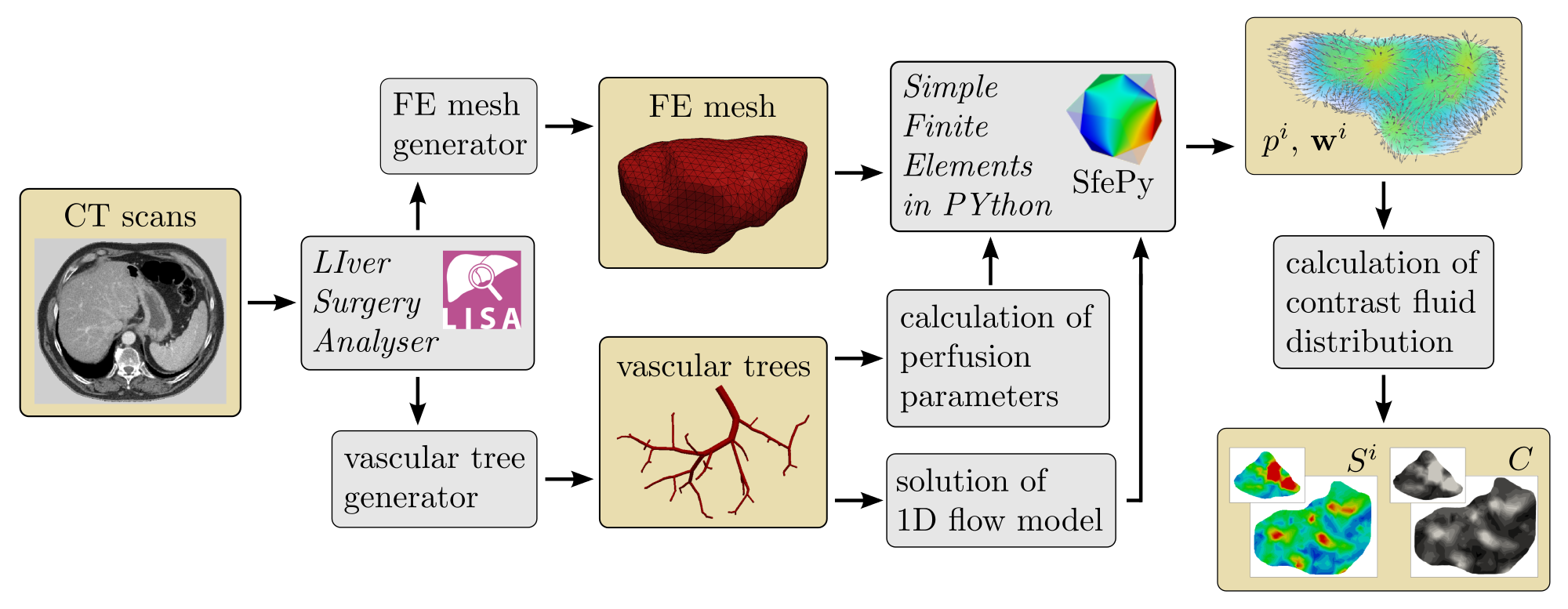
CT scans of human liver processed by the LISA (LIver Surgery Analyser) software (Jiřík, 2013–2015) are the starting point to the numerical simulation of liver perfusion. The LISA code includes the semi-automated segmentation method based on the graph-cut algorithm and returns the geometrical model of liver parenchyma that can be transformed into a volumetric finite element mesh. The code is also used to identify the position and diameter of the portal and hepatic veins at the point of entry into the liver parenchyma; this data is necessary to generate two artificial vascular trees associated with the portal and hepatic veins, which in part are employed directly in the simulation of the upper-level flow using the 1D flow model described in Section 2.3, but also to establish permeabilities and perfusion coefficients appearing in the multicompartment Darcy flow model. The hepatic artery is not considered in our liver model because of its small contribution to the overall blood perfusion through the liver tissue. A constrained constructive optimization approach is used for the creation of vascular structures reflecting main physiological principles, see Georg et al (2010), and the geometry of a particular liver.
In accordance with the modeling principles described above, the calculation of blood perfusion and contrast fluid distribution in the liver can be divided into two stages. The first one includes the solution of 1D flow model (11)-(12) coupled with the multicompartment Darcy model (10). The resulting velocities associated with vessel segments of the 1D flow model and velocity fields in compartments are then employed in the second stage in which the compartmental saturations yielding the total concentration are computed. The 1D flow model is implemented in the Python language, the multicompartment Darcy flow model is discretized using the FE method in software SfePy – Simple Finite Elements in Python, see Cimrman (2014). The model describing the tracer transport is implemented using the finite volume method in the Matlab system. The overview of the simulation process is illustrated in Fig. 4.
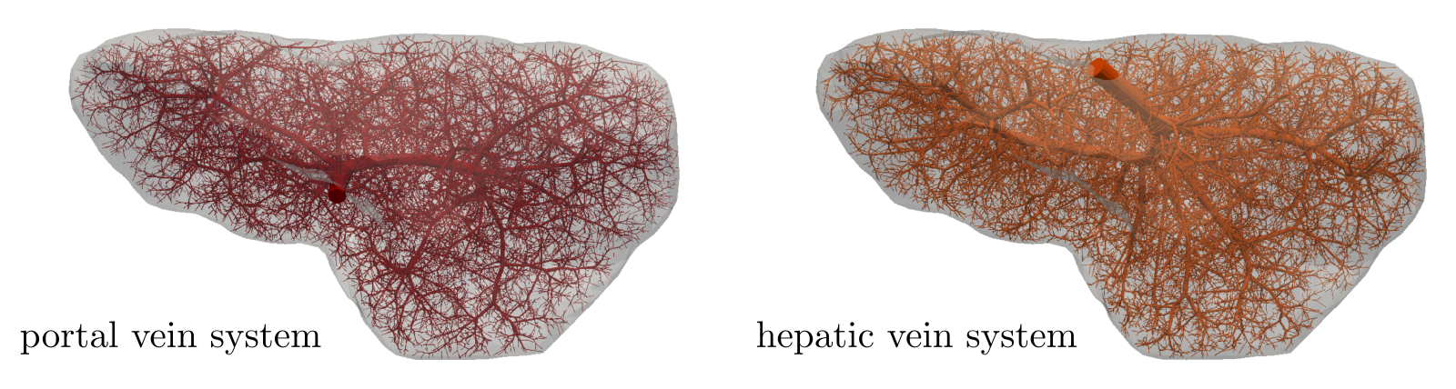
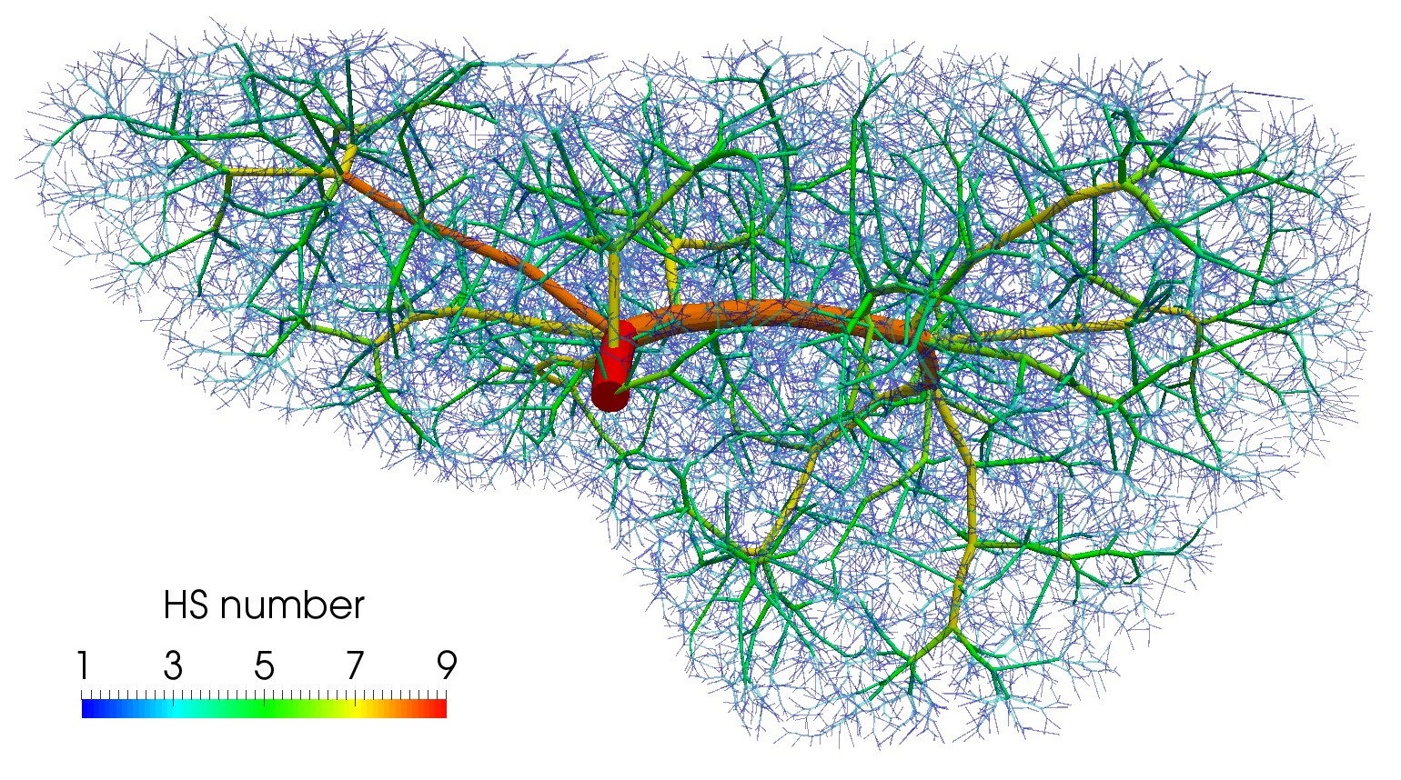
To demonstrate features of the hierarchical model described in this paper, a three compartment model is considered. The first compartment represents the vascular network of the portal vein consisting of veins with diameter in the range of about m. The same diameter range is chosen also for the third compartment which stands for the system of the hepatic vein. Compartment 2 involves small veins of diameters smaller than m including the hepatic capillaries of the lobular sinusoids, and it may therefore be perceived as a filtration part of the perfusion model. The generated artificial vascular trees representing the vascular networks in the liver are depicted in Fig. 5, their properties are summarized in Tab. 1. The higher hierarchy trees, where the blood flow is approximated by the 1D model, see Fig. 1, are obtained by taking the vessel segments with the Horton–Strahler (HS) number (Georg et al, 2010) greater or equal to 6. The branching complexity of the generated portal vascular tree characterized by the HS number is illustrated in Fig. 6.
| vascular | number of all | number of | diameter of | diameter of |
| tree | vessel segments | terminal segments | the root segment | terminal segments |
| portal | 36 739 | 19 777 | 8.4 mm | mm |
| hepatic | 37 133 | 19 769 | 5.8 mm | mm |
To determine parameters , and , , as well as the porosities , in each finite element, a volume averaging is performed over the corresponding vascular tree for a given range of the vessel diameters. The anisotropic permeabilities , of compartments 1 and 3 are evaluated using the expression derived by Huge and van Campen (Huyghe and Campen, 1995), whereas the coupling perfusion coefficients , are calculated with the help of the theory presented in Hyde et al (2013). Values of the model parameters at two selected points are listed in Tab. 2. The isotropic permeability in compartment 2 is taken as and the uniform porosity as , both values are chosen with respect to the parameters identified in Debbaut et al (2012). The domain of the liver is discretized by a finite element mesh consisting of 11 019 tetrahedrons and 2 442 nodes. The rather coarse mesh was chosen due to large computational cost associated with the tracer transport calculation.
| point | permeability [m(Pas)-1] | porosity [–] | coef. [(Pas)-1] |
|---|---|---|---|
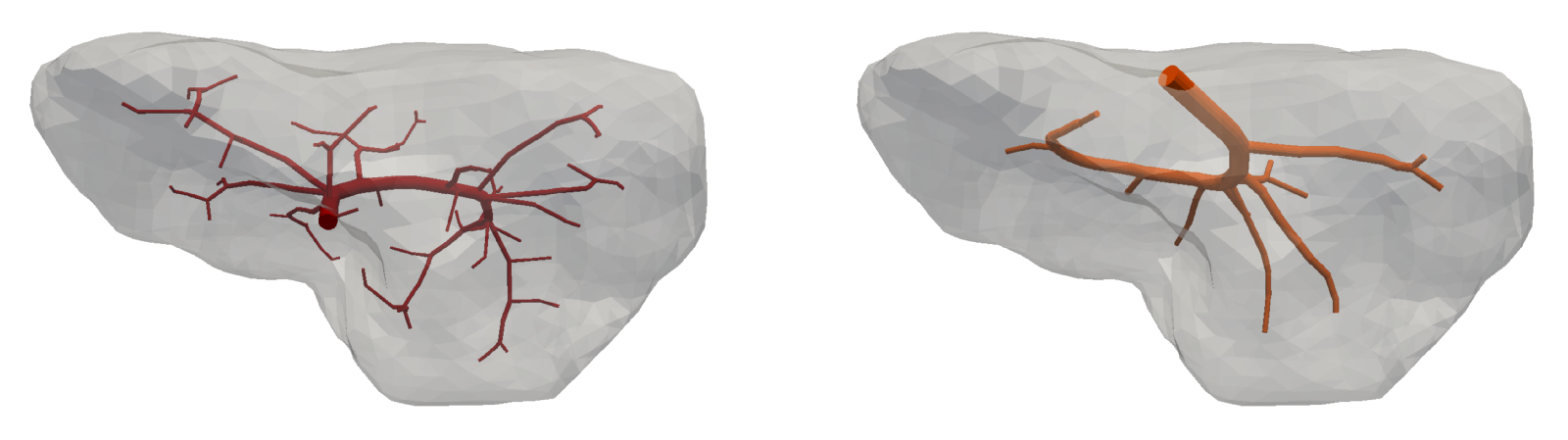
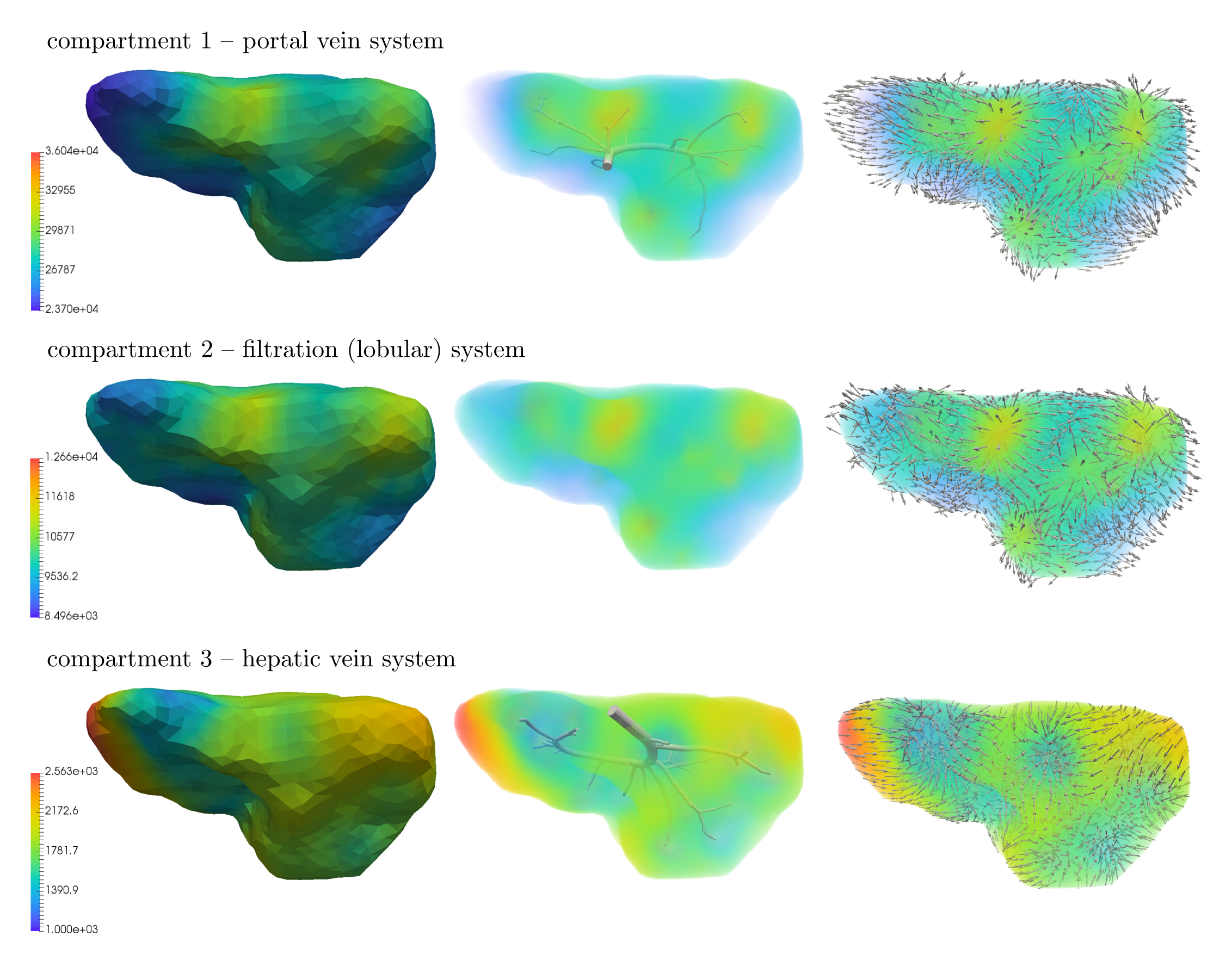
The 1D flow model is connected to the multicompartment model through 45 junctions, 34 of them are the sources located in compartment 1 and remaining 11 are the sinks located in compartment 3. The upper-level vascular trees, terminal points of which correspond to the sources and sinks, are shown in Fig. 7 and Fig. 8 (middle). The input blood velocity to the portal vein is taken as and the output blood pressure prescribed in the hepatic vein is Pa.
The steady state results computed for the three compartment perfusion model described above are presented in Fig. 8. This figure shows the distribution of pressure in each of the three compartments, (1 – portal, 2 – filtration, 3 – hepatic) as well as the corresponding velocity vectors , which well illustrate an interplay between the filling and draining functionality of the portal and hepatic compartments, respectively. From the surface and volumetric visualizations of the computed pressure fields (left, middle), it can be noticed that the portal (top) and hepatic (bottom) pressures depend strongly on the structure of the vascular trees, especially their upper-level hierarchies; this is in accordance with observations made on real human liver.
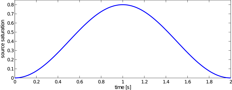
To get a better idea on how the different perfusion properties of the three compartments influence the final distribution of blood within the liver and also to simulate a real dynamic perfusion test, a simulation of the contrast fluid transport is carried out using the model presented in Section 3. For this purpose, a given external source saturation is prescribed in the form of a time bolus defined at the root segment of the portal vein system, Fig. 9,
| (28) |
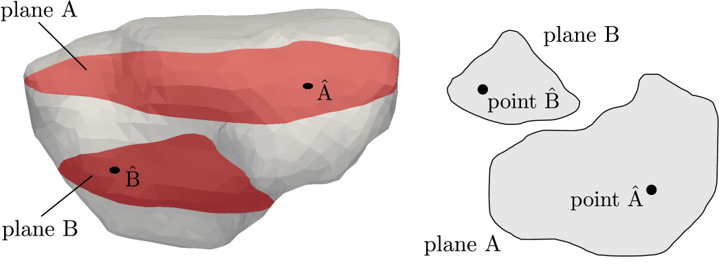
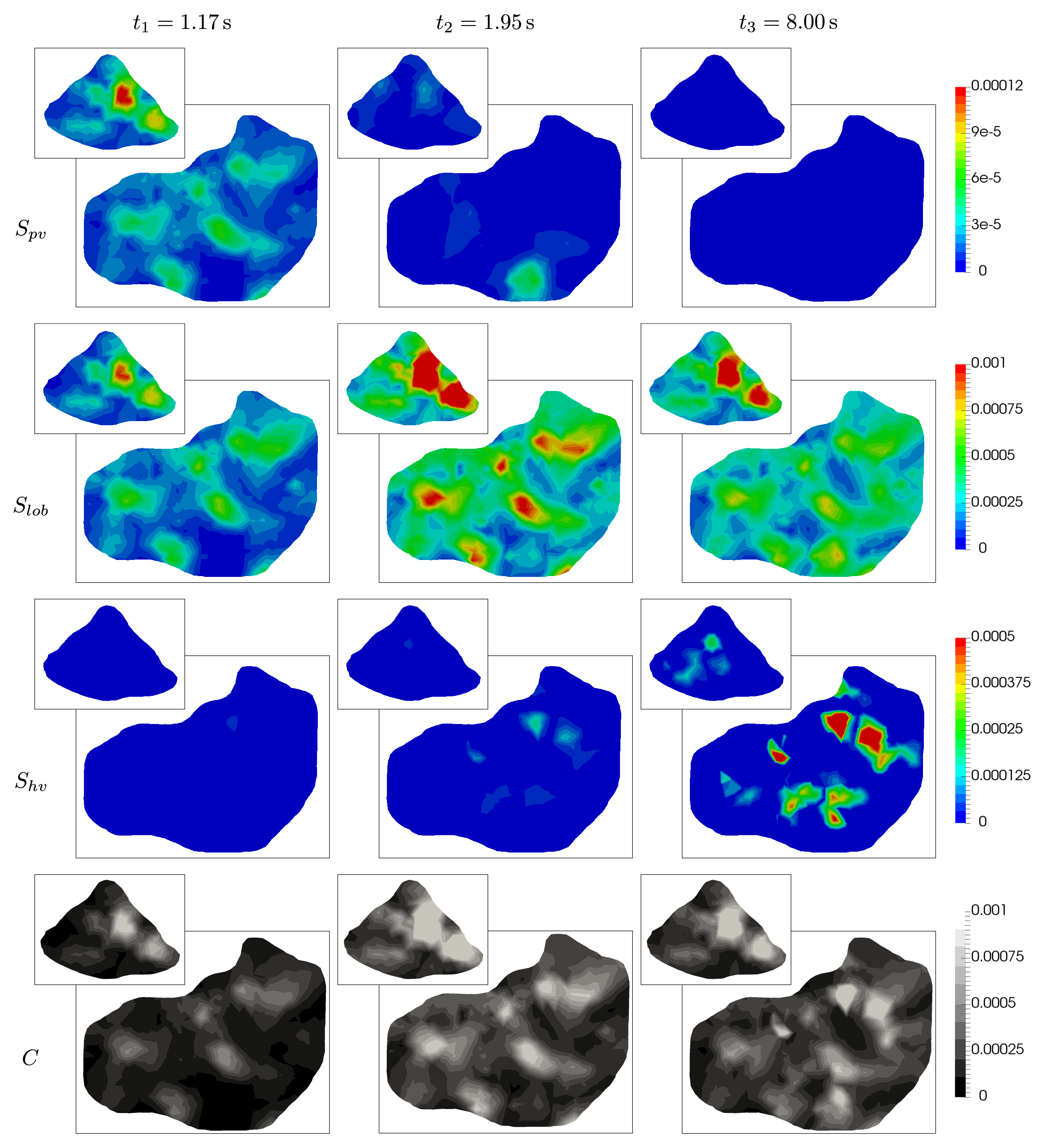
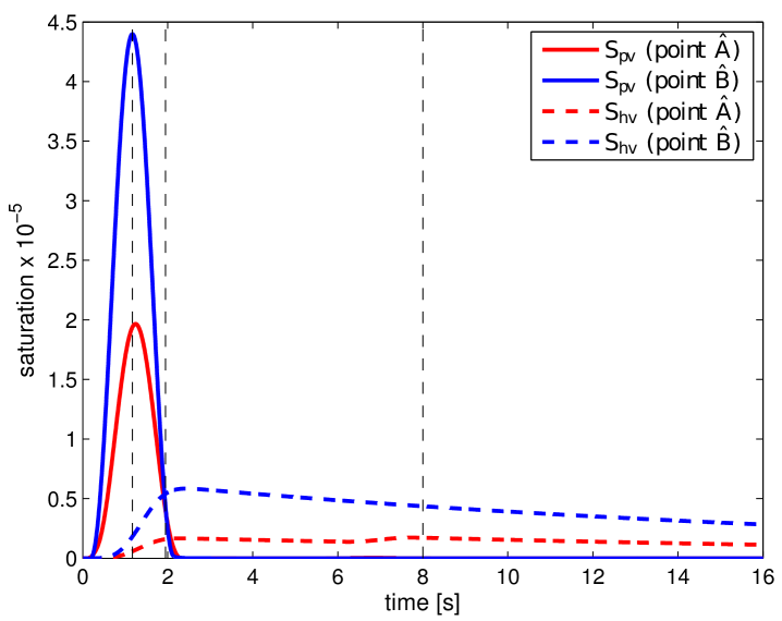
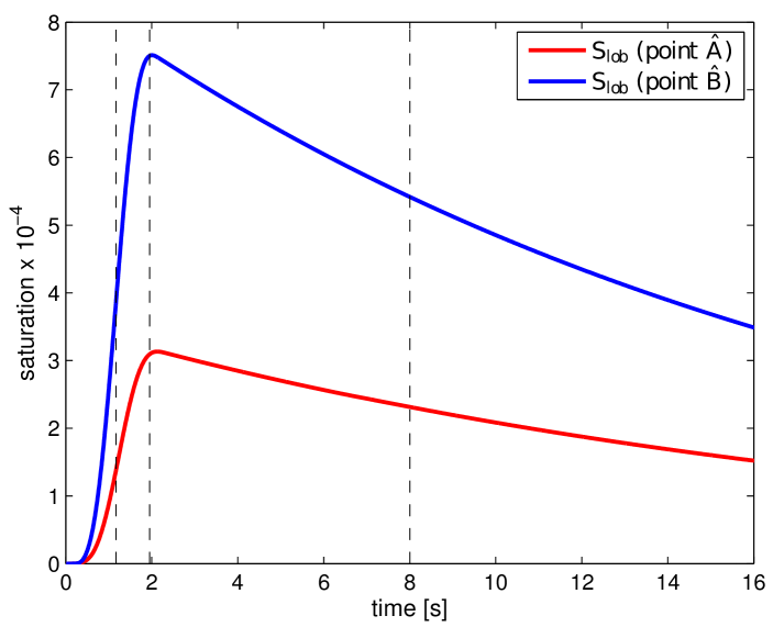
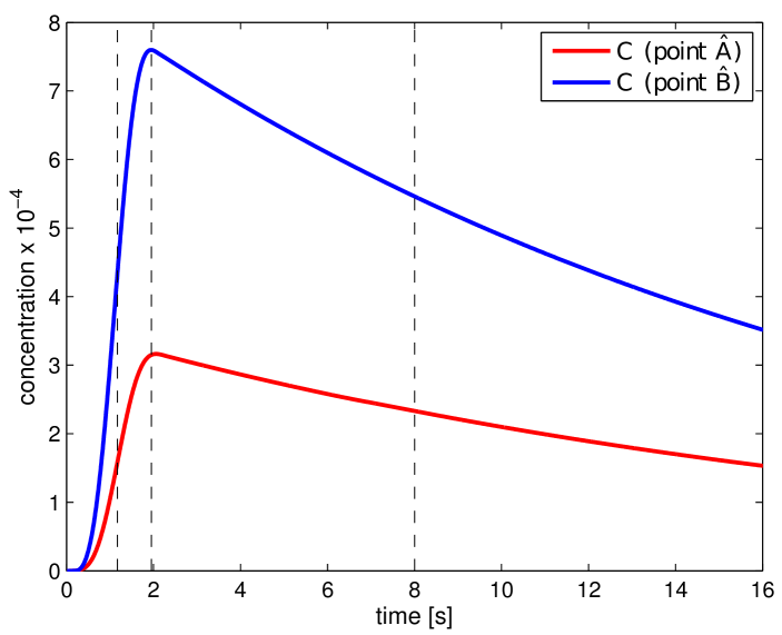
where and . In Fig. 11, the obtained portal , lobular and hepatic saturations and total apparent concentration are shown in two selected sections of the liver, positions of which are outlined in Fig. 10 and denoted as planes A and B. Due to the time-dependent character of the tracer transport simulation, the results in Fig. 11 are visualized at three time instants (, , and ). Note that the first two time instants reflect the time at which most of the portal and lobular saturations attain their maximum, see graphs in Fig. 12. The top graphs show the time development of the portal , hepatic and lobular saturations at points and located in planes A and B (Fig. 10), while the bottom graph depicts the evolution of the total apparent concentration at the same points.
The saturation isocontours presented in Fig. 11 clearly demonstrate the transport of the contrast fluid through each of the three considered liver compartments. In other words, the most apparent saturation of the respective compartment occurs successively—first in the portal vein system at the time , followed by the lobular one at and then concluded in the hepatic vein system at . This dynamics of the perfusion can also be recognized from the varying grey levels of the total apparent concentration in Fig. 11.
To get another, more time continuous view of the tracer transport through each of the three compartments, we refer to the graphs in Fig. 12; from there it is possible to observe a relatively fast “filtration” of the tracer through the portal compartment ( reaches its maximum shortly after the saturation bolus have entered the compartment; moreover, the shape of the bolus remains almost unchanged over time, see Fig. 12 (top left). On contrary, the filtration compartment, which is characterized by a relatively high porosity () compared to the ones computed in the filling/draining compartments ( and , see Tab. 2), fulfills its function as a filtration system, in which the saturation decreases only slowly over time, see Fig. 12 (top right). As a consequence, the perfusion properties of the filtration system influence the time development of the hepatic saturation which, compared to the portal saturation , changes much more gradually depending on tracer transfer from the filtration system.
Liver model with pathologically changed permeability
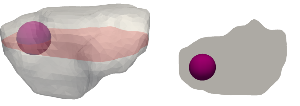
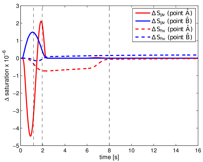
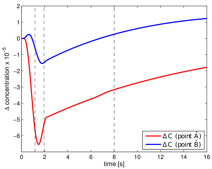
To demonstrate the applicability of the proposed model for numerical simulation of various liver tissue pathologies, a simple illustrative example is presented. In a small spherical region, which is depicted in Fig. 13, the permeability parameter of compartment 2 is locally changed to values close to zero (due to numerical reasons arising from the solution of the Darcy system). This change in permeability should mimic a pathology of the lobular structure, namely a lesion.
To be able to quantify how the introduction of the lesion within the parenchyma affects the overall perfusion of the liver including the transport of the contrast fluid, the following auxiliary quantities are introduced:
| (29) |
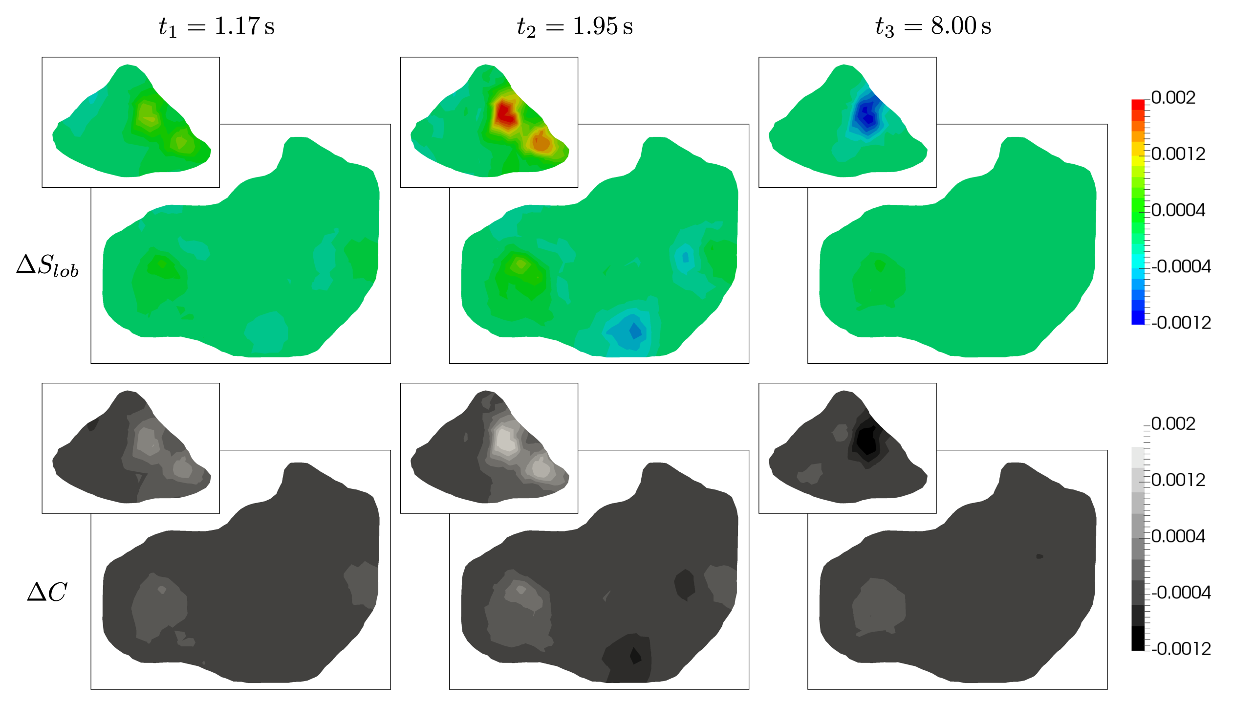
where the upper index “∙” denotes a quantity associated with the pathologically changed liver model. Similarly to Fig. 11, Fig. 14 shows the distribution of and in planes A and B at the three previously introduced time instants (, , and ). From the isocontours, it can be deduced that the lesion, which is located in the upper part of the liver model (near plane A), affects the perfusion and tracer transport globally. This phenomenon can be particularly observed on plane B, where at the beginning of the simulation () the lobular saturation of the original model is higher than in the case of the model with lesion (i.e., ). The presence of the lesion within the liver model and its influence on the overall blood perfusion is also reflected by the distribution of in Fig. 14 (bottom). Here the differences in the total concentration are apparent on both planes A and B. The region with in the left part of plane A is of particular importance, as it is clearly distinguishable in all snapshots, thus, indicating the location of the lesion.
To assess the impact of the lesion on the perfusion results in a time-continuous manner, we refer to the graphs shown in Fig. 15, which capture evolution of , and in time at the points and previously introduced. Note that, in comparison with Fig. 12, the graph of is not displayed in Fig. 15, as it would closely resemble that of . When comparing the plotted curves, two observations are worth of nothing. First, although the perfusion anomaly (lesion) is located only in the filtration compartment, it influences the perfusion and, thereby, the tracer transport through the higher hierarchies included in to the portal compartment (the difference is not zero from the beginning, i.e. for ). Second, curves plotted for the selected points and are dissimilar each other, no common features are evident. This is particularly apparent in the case of , which for both points exhibit completely different behaviour: On one hand, at point (red solid line in Fig. 12 (left)), the graph is characterized by a delayed maximum portal saturation in the undamaged liver model (fast change of from negative to positive values within a short time interval). On the other hand, the time evolution of at point (blue solid line in Fig. 12 (left)) shows no time delay, only higher portal saturation compared to the damaged liver model is apparent ( during the whole simulation). Similar observations can be made in the case of the and curves.
5 Conclusions
In the paper, we proposed the multicompartment model of the tissue blood perfusion and of the superimposed time-space distribution of the contrast fluid. This latter feature enables to establish a modeling feedback which is necessary to tune the model parameters according to information available due to standard clinical CT examination combined with essential flow parameters and basic structural and morphological data of a specific perfused tissue. Although the model is intended and currently being developed for modeling the liver perfusion, it can be adapted for other applications, namely the cerebral perfusion; this issue is in our focus for future work.
5.1 Summary of the proposed modeling approach
The perfusion model has been derived on a very simple idea of decomposing the perfusion tree into a number of sets – the compartments – which are hierarchically organized. The flow within each compartment is governed by the Darcy law involving permeability tensors . Cross links between two “communicating” compartments and is respected locally by scalar perfusion coefficients which are associated with cuts of the perfusion tree at those bifurcations separating the two different hierarchies. These features represent a substantial step towards an anatomically parametrized porous perfusion model. However, the key issue is the quantification of the model parameters. If an exact geometry of the perfusion tree is known, as in our case, when using the artificially generated trees, the permeabilities can be determined using the geometrical data by a representative volume averaging following the approaches suggested in Huyghe and Campen (1995); Vankan et al (1997) and followed in Hyde et al (2013). Following this work, a procedure has been proposed to determine also the perfusion coefficients which, however, would require resolving the whole “non-reduced” problem of flow on all vessel segments of the tree. Therefore, in our treatment, we simplified such a complex procedure to obtain an approximate, but tractable computation of the perfusion coefficients.
Flow on the uppermost hierarchies of the perfusion tree is described by the Bernoulli type model on 1D branching network; its coupling with the 3D continuum multicompartment model is by means of distributed point sources, or sinks. An iterative algorithm is based on commuting the 1D flow solvers associated with the portal and hepatic vein trees, and the 3D perfusion solver, whereby the inlet velocity at the portal vein is being increased gradually from zero until a steady state is reached.
As the second contribution of the paper, we propose the model describing the contrast fluid (the tracer) dynamic transport at all hierarchies of the perfusion trees. Superposition of the local saturation of the tracer in all compartments yields the local concentration, often called the tissue density which can be measured by the perfusion CT examination. On one hand, due to this option, it is possible to use the patient-specific CT images to tune the model parameters. On the other hand, this computational tool will allow for a deeper analysis of CT scans and a more accurate localization and assessment of possible liver pathology.
5.2 Discussion and future development of the model
To bring the modeling approach to its practical application with valuable outputs for clinical practice, there are several important issues to be pursued in our future work. The main purpose of using the multicompartment continuum model to describe approximately the flow on complex branching vessel networks, like trees, is to avoid direct flow simulations which may be prohibitively expensive and even non-feasible to provide real time solutions.
To verify the model performance, we need to check how the tree decomposition into varying number of compartments influences the modeling error. Such a numerical experiment requires a reference model which would provide a sufficiently fine and robust resolution of flow on all the vascular tree branches. For this purpose, we shall consider the 1D flow on the perfusion tree described by the Bernoulli-type model. This reference model will also be used to set the parameters for a particular split of the tree.
For practical use of the model, its parameters cannot be set appropriately using the direct calculations: the reason is twofold. If real data is used, the tree cannot be identified to a sufficient resolution of small vessels using the imaging techniques which are currently available. Moreover, even if the tree is known, as in our numerical examples, a cumbersome direct calculation of the flow would be necessary to set the parameters . Therefore, we intend to identify the model parameters by solving an inverse problem. In Rohan et al (2015a), we suggested a formulation of the nonlinear least square problem which is based on the discrepancy between the local contrast fluid concentration resolved by the model, and the corresponding data provided by the CT examination. This approach seems to be the only way of tuning the model. However, such a treatment requires further improvements of the model itself to capture more accurately the flow at the lowermost level of the parenchyma and also to account for dispersion of the contrast fluid during its transport through the compartments.
We are currently working on a homogenized model (Rohan et al, 2015b) of the flow on the capillary and pre-capillary level which should be integrated in the multicompartment model. In liver, the lobular level of the vasculature can be approximated by a periodic structure featured by the double porosity in the context of the vertex and the central venules connected by the hepatic capillaries of the sinusoids. Another issue is certainly related to the deformation of the parenchyma (Cimrman and Rohan, 2007; Rohan and Cimrman, 2010; Rohan and Lukeš, 2014). In a longer perspective, this phenomenon must be treated in the model to capture processes of the tissue remodeling.
Acknowledgements: This research is supported by the project LO 1506 of the Czech Ministry of Education,Youth and Sports.
References
- Bonfiglio et al (2010) Bonfiglio A, Leungchavaphongse K, Repetto R, Siggers JH (2010) Mathematical modeling of the circulation in the liver lobule. J Biomech Eng 132(11):111,011. doi: 10.1115/1.4002563
- Brůha et al (2015) Brůha J, Vyčítal O, Tonar Z, Mírka H, Haidingerová L, Beneš J, Pálek R, Skála M, Třeška V, Liška V (2015) Monoclonal antibody against transforming growth factor beta 1 does not influence liver regeneration after resection in large animal experiments. In Vivo 29(3):327–340
- Cimrman (2014) Cimrman R (2014) SfePy - write your own FE application. In: de Buyl P, Varoquaux N (eds) Proc 6th Eur Conf Python Sci (EuroSciPy 2013), pp 65–70
- Cimrman and Rohan (2007) Cimrman R, Rohan E (2007) On modelling the parallel diffusion flow in deforming porous media. Math Comput Simul 76:34–43. doi: 10.1016/j.matcom.2007.01.034
- Dai et al (2016) Dai W, Astary GW, Kasinadhuni AK, Carney PR, Mareci TH, Sarntinoranont M (2016) Voxelized model of brain infusion that accounts for small feature fissures: comparison with magnetic resonance tracer studies. J Biomech Eng 138(5), doi: 10.1115/1.4032626
- D’Angelo (2007) D’Angelo C (2007) Multiscale modelling of metabolism and transport phenomena in living tissues. PhD thesis, EPFL, Lausanne. doi: 10.5075/epfl-thesis-3803
- Debbaut et al (2014) Debbaut C, Segers P, Cornillie P, Casteleyn C, Dierick M, Laleman W, Monbaliu D (2014) Analyzing the human liver vascular architecture by combining vascular corrosion casting and micro-CT scanning: a feasibility study. J Anat 224(4):509–517. doi: 10.1111/joa.12156
- Debbaut et al (2012) Debbaut C, Vierendeels J, Casteleyn C, Cornillie P, Van Loo D, Simoens P, Van Hoorebeke L, Monbaliu D, Segers P (2012) Perfusion characteristics of the human hepatic microcirculation based on three-dimensional reconstructions and computational fluid dynamic analysis. J Biomech Eng 134(1):011,003, doi: 10.1115/1.4005545
- Fieselmann et al (2011) Fieselmann A, Kowarschik M, Ganguly A, Hornegger J, Fahrig R (2011) Deconvolution-based CT and MR brain perfusion measurement: theoretical model revisited and practical implementation details. J Biomed Imaging 2011:14. doi: 10.1155/2011/467563
- Formaggia et al (2009) Formaggia L, Quarteroni A, Veneziani A (2009) Cardiovascular Mathematics: Modeling and Simulation of the Circulatory System. Springer
- Georg et al (2010) Georg M, Preusser T, Hahn HK (2010) Global constructive optimization of vascular systems. Tech. Rep. 2010-11, Washington University in St. Louis
- Huyghe and Campen (1995) Huyghe JM, Campen DH (1995) Finite deformation theory of hierarchically arranged porous solids, part I.,II. Int J Eng Sci 33(13):1861–1886
- Hyde et al (2013) Hyde ER, Michler C, Lee J, Cookson AN, Chabiniok R, Nordsletten DA, Smith NP (2013) Parameterisation of multi-scale continuum perfusion models from discrete vascular networks. Med Biol Eng Comput 51(5):557–570. doi: 10.1007/s11517-012-1025-2
- Jiřík (2013–2015) Jiřík M (2013–2015) Lisa – computer aided liver surgery. https://github.com/mjirik/lisa
- Jonášová et al (2014) Jonášová A, Bublík O, Vimmr J (2014) A comparative study of 1d and 3d hemodynamics in patient-specific hepatic portal vein networks. Appl Comput Mech 8(2):177–186
- Jonášová et al (2014) Jonášová A, Rohan E, Lukeš V, Bublík O (2014) Complex hierarchical modeling of the dynamic perfusion test: application to liver. In: 11th World Congr Comput Mech (WCCM XI)
- Keeling et al (2007) Keeling SL, Bammer R, Stollberger R (2007) Revision of the theory of tracer transport and the convolution model of dynamic contrast enhanced magnetic resonance imagingrevision of the theory of tracer transport and the convolution model of dynamic contrast enhanced magnetic resonance imaging. J Math Biol 55(3):389–411, doi: 10.1007/s00285-007-0089-3
- Koh et al (2006) Koh TS, Tan CKM, et al (2006) Cerebral perfusion mapping using a robust and efficient method for deconvolution analysis of dynamic contrast-enhanced images. NeuroImage 33:570–579. doi: 10.1016/j.neuroimage.2006.03.042
- Lettmann and Hardtke-Wolenski (2014) Lettmann KA, Hardtke-Wolenski M (2014) The importance of liver microcirculation in promoting autoimmune hepatitis via maintaining an inflammatory cytokine milieu–a mathematical model study. J Theor Biol 348:33–46. doi: 10.1016/j.jtbi.2014.01.016
- Liška et al (2012) Liška V, Třeška V, Mírka H, Beneš J, Vyčítal O, Brůha J, Pitule P, Skalický T, Sutnar A, Chlumská A, Racek J, Trefil L, Fínek J, Holubec L (2012) Immediately preoperative use of biological therapy does not influence liver regeneration after large resection - porcine experimental model with monoclonal antibody against epidermal growth factor. In Vivo 26:683–691
- Lukeš et al (2014) Lukeš V, Jiřík M, Jonášová A, Rohan E, Bublík O, Cimrman R (2014) Numerical simulation of liver perfusion: from CT scans to FE model. In: de Buyl P, Varoquaux N (eds) Proc 7th Eur Conf Python Sci (EuroSciPy 2014)
- Materne et al (2000) Materne R, Beers BEV, Smith AM, Leconte I, Jamart J, Dehoux JP, Keyeux A, Horsmans Y (2000) Non-invasive quantification of liver perfusion with dynamic computed tomography and a dual-input one-compartmental model. Clin Sci 99:517–525
- Mehrabian and Abousleiman (2014) Mehrabian A, Abousleiman YN (2014) Generalized Biot’s theory and Mandel’s problem of multiple-porosity and multiple-permeability poroelasticity. J Geophys Res: Solid Earth 119:2745–2763. doi: 10.1002/2013JB010602
- Mescam et al (2010) Mescam M, Kretowski M, Bezy-Wendling J (2010) Multiscale model of liver dce-mri towards a better understanding of tumor complexity. IEEE Trans Med Imaging 29:699–707. doi: 10.1109/TMI.2009.2031435
- Michler et al (2013) Michler C, Cookson AN, Chabiniok R, Hyde ER, Lee J, Sinclair M, Sochi T, Goyal A, Vigueras F, Nordsletten DA, Smith NP (2013) A computationally efficient framework for the simulation of cardiac perfusion using a multi-compartment darcy porous-media flow model. Int J Numer Methods in Biomed Eng 29(2):217–232. doi: 10.1002/cnm.2520
- Peterlik et al (2012) Peterlik I, Duriez C, Cotin S (2012) Modeling and real-time simulation of a vascularized liver tissue. Med Image Comput Comput Assist Interv 15:50–57
- Plantefèv et al (2016) Plantefèv R, Peterlik I, Haouchine N, Cotin S (2016) Patient-specific biomechanical modeling for guidance during minimally-invasive hepatic surgery. Ann Biomed Eng 44(1):139–153, doi: 10.1007/s10439-015-1419-z
- Pozrikidis (2010) Pozrikidis C (2010) Numerical simulation of blood and interstitial flow through a solid tumor. J Math Biol 60(1):75–94, doi: 10.1007/s00285-009-0259-6
- Reichold (2011) Reichold J (2011) Cerebral blood flow modeling in realistic cortical microvascular networks. PhD thesis, ETH, Zürich, doi: 10.3929/ethz-a-007146515
- Reichold et al (2009) Reichold J, Stampanoni M, Lena Keller A, Buck A, Jenny P, Weber B (2009) Vascular graph model to simulate the cerebral blood flow in realistic vascular networks. J Cerebr Blood Flow Metab 29(8):1429–1443, doi: 10.1038/jcbfm.2009.58
- Ricken et al (2010) Ricken T, Dahmen U, Dirsch O (2010) A biphasic model for sinusoidal liver perfusion remodeling after outflow obstruction. Biomech Model Mechanobiol 9(4):435–450. doi: 10.1007/s10237-009-0186-x
- Ricken et al (2015) Ricken T, Werner D, Holzhütter H, König M, Dahmen U, Dirsch O (2015) Modeling function-perfusion behavior in liver lobules including tissue, blood, glucose, lactate and glycogen by use of a coupled two-scale pde-ode approach. Biomech Model Mechanobiol 14(3):515–536. doi: 10.1007/s10237-014-0619-z
- Rohan and Cimrman (2010) Rohan E, Cimrman R (2010) Two-scale modelling of tissue perfusion problem using homogenization of dual porous media. Int J Multiscale Comput Eng 8:81–102
- Rohan and Lukeš (2014) Rohan E, Lukeš V (2014) On modelling nonlinear phenomena in deforming heterogeneous media using homogenization and sensitivity analysis concepts. Proc 12th Int Conf Comput Struct Technol pp 1–20
- Rohan et al (2015a) Rohan E, Lukeš V, Brašnová J (2015a) CT based identification problem for the multicompartment model of blood perfusion. In: Proc V ECCOMAS Thematic Conf Comput Vis Med Image Process: VipIMAGE 2015, Taylor and Francis, Tenerife, Spain
- Rohan et al (2012a) Rohan E, Lukeš V, Jonášová A (2012a) Modeling of dynamic perfusion test using a two-scale model of tissue parenchyma with layer-wise decomposition. In: ECCOMAS 2012 – Eur Congres Comput Methods Appl Sci Eng, pp 2733–2743
- Rohan et al (2012b) Rohan E, Naili S, Cimrman R, Lemaire T (2012b) Multiscale modeling of a fluid saturated medium with double porosity: Relevance to the compact bone. J Mech Phys Solids 60:857–881. doi: 10.1016/j.jmps.2012.01.013
- Rohan et al (2015b) Rohan E, Turjanicová J, Lukeš V (2015b) Modelling flows in multi-porous media using homogenization with application to liver lobe perfusion. In: Kruis J, Tsompanakis Y, Topping B (eds) Proc 15th Int Conf Civil Struct Environ Eng Comput, Civil-Comp Press, Stirlingshire, UK, pp 108–148
- Ryba et al (2013) Ryba T, Jiřík M, Železný M (2013) An automatic liver segmentation algorithm based on grow cut and level sets. Pattern Recognit Image Anal 23(4):1054–6618
- Schneider et al (2012) Schneider M, Reichold J, Weber B, Sz kely G, Hirsch S (2012) Tissue metabolism driven arterial tree generation. Medical Image Analysis 16(7):1397–1414
- Schwen and Preusser (2012) Schwen LO, Preusser T (2012) Analysis and algorithmic generation of hepatic vascular systems. Int J Hepatol 2012. doi: 10.1155/2012/357687
- Shipley and Chapman (2010) Shipley RJ, Chapman SJ (2010) Multiscale modelling of fluid and drug transport in vascular tumours. Bull Math Biol 72(6):1464–1491. doi: 10.1007/s11538-010-9504-9
- Showalter and Visarraga (2004) Showalter R, Visarraga D (2004) Double-diffusion models from a highly heterogeneous medium. J Math Anal Appl 295(1):191–210. doi: 10.1016/j.jmaa.2004.03.031
- Siggers et al (2014) Siggers JH, Leungchavaphongse K, Ho CH, Repetto R (2014) Mathematical model of blood and interstitial flow and lymph production in the liver. Biomech Model Mechanobiol 13(2):363–378. doi: 10.1007/s10237-013-0516-x
- Slattery (1967) Slattery JC (1967) Flow of viscoelastic fluids through porous media. AIChE Journal 13:1066–1071. doi: 10.1002/aic.690130606
- Tonar et al (2015) Tonar Z, Kubíková T, Prior C, Demjèn E, Liška V, Králíčková M, Witter K (2015) Segmental and age differences in the elastin network, collagen, and smooth muscle phenotype in the tunica media of the porcine aorta. Ann Anat 201:79–90, doi: 10.1016/j.aanat.2015.05.005
- Třeška et al (2014) Třeška V, Liška V, Fichtl J, Lysák D, Mírka H, Brůha J, Duras P, Trešková I, Náhlík J, Šimánek V, Topolčan O (2014) Portal vein embolisation with application of haematopoietic stem cells in patients with primarily or non-resectable colorectal liver metastasesportal vein embolisation with application of haematopoietic stem cells in patients with primarily or non-resectable colorectal liver metastases. Anticancer Res 34(12):7279–7285
- Vankan et al (1997) Vankan W, Huyghe J, Janssen J, Huson A, Hacking W, Schreiner W (1997) Finite element analysis of blood flow through biological tissue. Int J Eng Sci 35(4):375–385. doi: 10.1016/S0020-7225(96)00108-5
- Whitaker (1967) Whitaker S (1967) Diffusion and dispersion in porous media. AIChE Journal 13(3):420–427. doi: 10.1002/aic.690130308