Modelling and Search-Based Testing of Robot Controllers Using Enzymatic Numerical P Systems

Due to the remarkable technological progress of late years, software applications tend to have a considerable role in solving most problems of everyday life. The medical, financial or automotive fields are just three of the main areas in which software products are intensively used. Given the importance of these areas in every individual’s life, ensuring product quality and functionality is an essential step in the development process. The safety of software systems for large-scale use is ensured by testing. Software testing aims to validate the fulfillment of the requirements defined for the developed product, as well as to identify possible unwanted behaviors triggered by simulating certain operational contexts.

In this paper, we propose an approach for testing two different lane keeping controllers designed to move an educational robot called E-puck [9]. Both controllers are based on numerical P systems, introduced by G. Păun and R. Păun in [12]. We also provide an equivalent version for the models using enzymatic numerical P systems, an extension of numerical P systems, defined by A. Pavel et al. in [10]. For this experiment we used some reliable tools which will be introduced in the following sections.

The paper is structured as described: Section 2 presents the P system variants to be used in the paper. Section 3 introduces the working environment, including the tools used. Section 4 describes the models and the main differences between them, while Section 5 illustrates the testing approach along with the results. In the end, Section 6 presents the future work and conclusions.

Membrane computing is a field of research introduced by Gh. Păun in [11, 13]. The computational paradigm was originally inspired by the structure and functionality of the living cells. Several classes of membrane systems (P systems) have been later defined and investigated, being classified according to the structure of the membranes as cell-like, tissue-like and neural-like P systems. Membrane computing has made significant breakthroughs in the last decades in fields like computer science, economics or biology. Depending on the requirements, extensions of the main concept were introduced and our experiment involves two of these types: numerical P systems and enzymatic numerical P systems.

In this section we will provide brief descriptions of the tools we integrated in our experiment. Firstly, we used an open-source software which allows the simulation of numerical P systems and enzymatic numerical P systems. The simulator is called PeP and will be introduced later in this section. Since we don’t have the physical education robot involved in this study, we also used a dedicated platform for robot simulations, called Webots. For tests generation, we used a tool which won the SBST Tool Competition 2022 [5]. We will discuss later in this section the arguments for using a search-based testing tool.

In this section we will present two models used to control the robot, the core of the controller. The controller receives data from proximity sensors, that measure distances to obstacles from the environment, to determine the direction of movement of a differential two wheeled robot, E-puck, in our case.

The proximity sensor has a range of 4 cm; if the obstacles are further than this limit the sensor returns the value of 0. The proximity sensors are placed on the left and right side of the robot in the direction of its movement at different angles.

The first model was taken from [4] and adapted. The equations that calculate the linear and angular velocity are shown below:

The $\mathit{leftSpeed}$ and $\mathit{rightSpeed}$ are the speeds of the two wheels of the robot. The enzymatic numerical P system described below encapsulates this behavior.
The first model is defined as follows:

where:

• •

  $\mathit{m=k\cdot 3+3,k=6}$, where $\mathit{k}$ is the number of proximity sensors;

• •

  $\mathit{H=\{s,s_{c}\}\cup\displaystyle\bigcup_{i=1}^{k}\{c_{i},s_{i},w_{i}\}}$;

• •

  $\mathit{\mu=[[[]_{s_{1}}[]_{w_{1}}]_{c_{1}}\dots[[]_{s_{k}}[]_{w_{k}}]_{c_{k}}[]_{s_{c}}]_{s};}$

• •

  $\mathit{Var_{s}=\{x_{s_{l}},x_{s_{r}}\},Var_{s_{c}}=\{x_{s_{c}}\},}$
  $\mathit{Var_{c_{i}}=\{x_{c_{i},s_{l}},x_{c_{i},s_{r}},x_{c_{i},w_{l}},x_{c_{i},w_{r}},e_{c_{i}}\},1\leq i\leq k,}$
  $\mathit{Var_{s_{i}}=\{x_{s_{i},i}\},1\leq i\leq k,}$
  $\mathit{Var_{w_{i}}=\{x_{w_{i},w_{l}},x_{w_{i},w_{r}},e_{w_{i}}\},1\leq i\leq}k$;

• •

  $\mathit{Var_{i}(0)=0,1\leq i\leq k}$;

• •

  $\mathit{Pr_{s}=\{0\cdot x_{s_{l}}\cdot x_{s_{r}}\rightarrow 1|x_{s_{l}}+1|x_{s_{r}}\}}$;
  $\mathit{Pr_{s_{c}}=\{3x_{s_{c}}\rightarrow 1|x_{s_{c}}+1|x_{s_{l}}+1|x_{s_{r}}\}}$;
  $\mathit{Pr_{c_{i}}=\{x_{c_{i},s_{l}}\cdot x_{c_{i},w_{l}}|_{e_{c_{i}}}\rightarrow 1|x_{s_{l}},}$
              $\mathit{x_{c_{i},s_{r}}\cdot x_{c_{i},w_{r}}|_{e_{c_{i}}}\rightarrow 1|x_{s_{r}}\},1\leq i\leq k}$;
  $\mathit{Pr_{s_{i}}=\{3x_{s_{i},i}\rightarrow 1|x_{s_{i},i}+1|x_{c_{i},s_{l}}+1|x_{c_{i},s_{r}}\},1\leq i\leq k}$;
  $\mathit{Pr_{w_{i}}=\{2x_{w_{i},w_{l}}|_{e_{w_{i}}}\rightarrow 1|x_{w_{i},w_{l}}+1|x_{c_{i},w_{l}},}$
              $\mathit{2x_{w_{i},w_{r}}|_{e_{w_{i}}}\rightarrow 1|x_{w_{i},w_{r}}+1|x_{c_{i},w_{r}}\},1\leq i\leq k}$;

The meaning of the variables from the model is the following:

• $\circ$

  $\mathit{x_{s_{l}}}$ and $\mathit{x_{s_{r}}}$ from the region $\mathit{s}$ represent $\mathit{leftSpeed}$ and $\mathit{rightSpeed}$, the sum of the products are accumulated in $\mathit{s}$ ;

• $\circ$

  $\mathit{x_{s_{c}}}$ from the compartment $\mathit{s_{c}}$ is $\mathit{cruiseSpeed}$;

• $\circ$

  each pair of weights, $\mathit{weightLeft_{i}}$ and $\mathit{weightRight_{i}}$, resides in the regions $\mathit{w_{i}}$, $\mathit{1\leq i\leq k}$;

• $\circ$

  for each proximity sensor, $\mathit{prox_{i}}$, a compartment is defined, namely $s_{i}$, containing a single variable, $\mathit{x_{s_{i},i}}$, $\mathit{1\leq i\leq k}$;

• $\circ$

  the products are calculated by two distinct programs, $\mathit{weightLeft_{i}\cdot prox_{i}}$, and $\mathit{weightRight_{i}\cdot prox_{i}}$, $\mathit{1\leq i\leq k}$, in the compartments $\mathit{c_{i}}$.

The second model is an improvement on the first one. First we define the function

This function will be used in the equations describing the behavior of the model and in the production functions from the programs.

The equations describing the behavior are:

The model is defined as follows:

where:

• •

  $\mathit{m=3k+3,k=6;}$

• •

  $\mathit{H=\{s,w,s_{c}\}\cup\displaystyle\bigcup_{i=1}^{k}\{c_{i},s_{i},w_{i}\}}$;

• •

  $\mathit{\mu=[[[[]_{s_{1}}[]_{w_{1}}]_{c_{1}}\dots[[]_{s_{k}}[]_{w_{k}}]_{c_{k}}[]_{s_{c}}]_{w}]_{s};}$

• •

  $\mathit{Var_{s}=\{x_{s_{l}},x_{s_{r}}\},Var_{w}=\{x_{w_{l}},x_{w_{r}},e_{w}\},Var_{s_{c}}=\{x_{s_{c}}\},}$
  $\mathit{Var_{c_{i}}=\{x_{c_{i},s_{l}},x_{c_{i},s_{r}},x_{c_{i},w_{l}},x_{c_{i},w_{r}},e_{c_{i}}\},1\leq i\leq k,}$
  $\mathit{Var_{s_{i}}=\{x_{s_{i},i}\},1\leq i\leq k,}$
  $\mathit{Var_{w_{i}}=\{x_{w_{i},w_{l}},x_{w_{i},w_{r}},e_{w_{i}}\},1\leq i\leq k}$;

• •

  $\mathit{Var_{i}(0)=0,1\leq i\leq k}$;

• •

  $\mathit{Pr_{s}=\{0\cdot x_{s_{l}}\cdot x_{s_{r}}\rightarrow 1|x_{s_{l}}+1|x_{s_{r}}\}}$;
  $\mathit{Pr_{w}=\{x_{s_{c}}\cdot x_{w_{l}}+f(x_{w_{l}})\cdot x_{s_{c}}|_{e_{w}}\rightarrow 1|x_{s_{l}},}$
              $\mathit{x_{s_{c}}\cdot x_{w_{r}}+f(x_{w_{r}})\cdot x_{s_{c}}|_{e_{w}}\rightarrow 1|x_{s_{r}}\}}$;
  $\mathit{Pr_{s_{c}}=\{x_{s_{c}}\rightarrow 1|x_{s_{c}}\}}$;
  $\mathit{Pr_{c_{i}}=\{x_{c_{i},s_{l}}\cdot x_{c_{i},w_{l}}|_{e_{c_{i}}}\rightarrow 1|x_{s_{l}},}$
              $\mathit{x_{c_{i},s_{r}}\cdot x_{c_{i},w_{r}}|_{e_{c_{i}}}\rightarrow 1|x_{s_{r}}\},1\leq i\leq k}$;
  $\mathit{Pr_{s_{i}}=\{3x_{s_{i},i}\rightarrow 1|x_{s_{i},i}+1|x_{c_{i},s_{l}}+1|x_{c_{i},s_{r}}\},1\leq i\leq k}$;
  $\mathit{Pr_{w_{i}}=\{2x_{w_{i},w_{l}}|_{e_{w_{i}}}\rightarrow 1|x_{w_{i},w_{l}}+1|x_{c_{i},w_{l}},}$
              $\mathit{2x_{w_{i},w_{r}}|_{e_{w_{i}}}\rightarrow 1|x_{w_{i},w_{r}}+1|x_{c_{i},w_{r}}\},1\leq i\leq k}$;

As we see from the definition of the $\varPi\mathit{{}_{M_{1}}}$ and its equations, in the proximity of an obstacle, roadside, the speed of the wheel on the side with the obstacle increases according to the weights. In certain circumstances, particularly related to the geometry of a tight road curve, the sum between travel speed and the weights results in a rotation in the opposite direction of the obstacle, but a slight forward motion still continues, causing the robot to leave the road.

The second model, $\varPi\mathit{{}_{M_{2}}}$, overcomes this problem by calculating the product of the travel speed and the sum of the weights. In a similar situation, the second model performs an angular rotation, in the opposite direction to the obstacle, and when the proximity sensors no longer detect obstacles, it continues moving forward with a constant velocity. This behavior is modeled by compartment $\mathit{w}$.

In the next section, it can be seen that the $\varPi\mathit{{}_{M_{2}}}$ model has better behavior in similar situations compared to the first model.

Having presented the way we integrate the tools along with the models we will detail in this section the testing stage. Ambiegen offers the possibility to configure the setup for its genetic algorithms, choosing the values for parameters like population size, number of generations, mutation rate or crossover rate. Also, aspects like the amount of time allocated for tests generation, map size, out of bound percent from which the test is considered as failed can be set easily from the command line, when executing the main Python file used in [5].

After series of trials we kept the default values, so we used the population size 100 with 75 generations. Mutation rate is 0.4 and crossover rate is 1. These values can be changed from the internal configuration file of Ambiegen. From the command line we chose the time budget allocated to generation and execution to be 1800 seconds and the map size to 200x200 meters which is the default value. For the out of bound percentage we also kept the default value (95%). After each simulation, Ambiegen exported roads spines coordinates as text files and we also plotted each generated road, as mentioned before. Then we could easily chose different roads based on the number of curves and their angle as the main criteria to diversify the tests that were supposed to be given to E-puck controller in Webots.

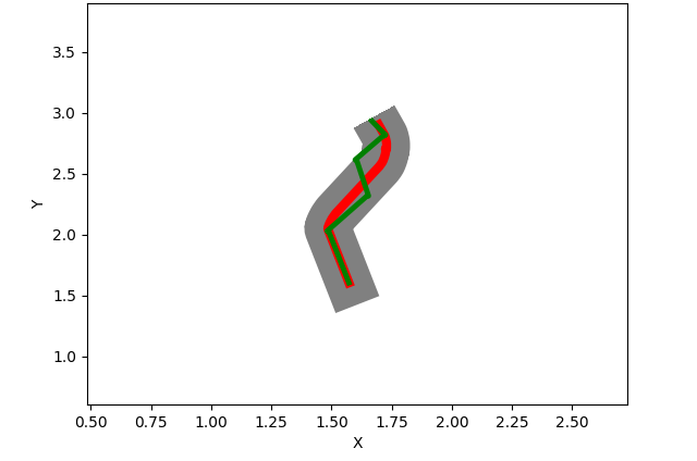
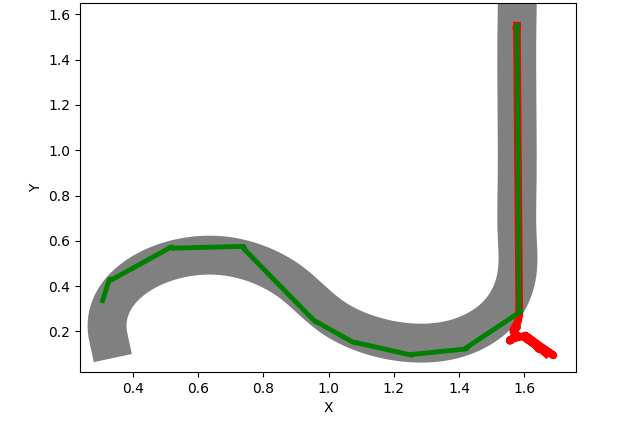
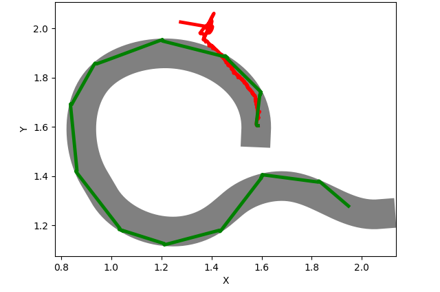
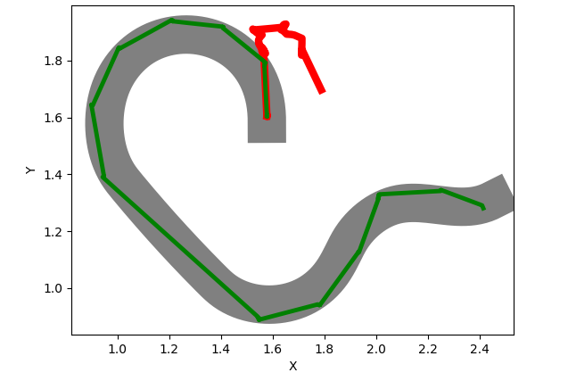
Next we report some roads along with the simulation results. The road is marked with grey, whilst the trajectory using the first model is represented with red. The trajectory of the second model (the improved one) is colored with green.

In Figure 1 we can see the results of different roads tests. We observe that Test 1, being the simplest test of the above presented, is passed by both models. In the next scenarios, the complexity of the road increases and only the improved model can pass.

From all the experiments, we noticed that the first model (the one marked with red in results) cannot pass a huge majority of tests with curves, whilst the improved model performs a rotation movement when the road is curved and for this reason it manages to advance until the end of the road. Additional tests were added to [16].

In this paper we presented an approach to test different enzymatic numerical P systems models using modern tools and search-based generated tests. We evaluated our approach on a research and educational robot called E-puck, virtually represented in Webots simulator. We set up our working environment incorporating the tools with different scripts created to ensure a smooth integration between them and also a better data processing. We formally described each model involved and then showed the differences between the lane-keeping controllers resulted when using each of them. As future work, we will investigate the possibility to dynamically calculate the values for weights, which are at the moment empirically assigned. Based on the controller behavior during the previous tests, the weights values will be automatically adapted. Also, we will try to develop a method to generate more complex roads in order to better challenge the controllers.

References

- [1]
- [2] Micael S Couceiro, Patricia A Vargas & Rui P Rocha (2014): Bridging the reality gap between the Webots simulator and e-puck robots. Robotics and Autonomous Systems 62(10), pp. 1549–1567, 10.1016/j.robot.2014.05.007.
- [3] Kalyanmoy Deb, Amrit Pratap, Sameer Agarwal & TAMT Meyarivan (2002): A fast and elitist multiobjective genetic algorithm: NSGA-II. IEEE transactions on evolutionary computation 6(2), pp. 182–197, 10.1109/4235.996017.
- [4] Andrei George Florea & Cătălin Buiu (2017): Modelling multi-robot interactions using a generic controller based on numerical P systems and ROS. In: 2017 9th International Conference on Electronics, Computers and Artificial Intelligence (ECAI), pp. 1–6, 10.1109/ECAI.2017.8166411.
- [5] Alessio Gambi, Gunel Jahangirova, Vincenzo Riccio & Fiorella Zampetti (2022): SBST tool competition 2022. In: Proceedings of the 15th Workshop on Search-Based Software Testing, pp. 25–32, 10.1145/3526072.3527538.
- [6] Dmytro Humeniuk, Giuliano Antoniol & Foutse Khomh (2022): AmbieGen tool at the SBST 2022 Tool Competition. In: Proceedings of the 15th Workshop on Search-Based Software Testing, pp. 43–46, 10.1145/3526072.3527531.
- [7] Dmytro Humeniuk, Foutse Khomh & Giuliano Antoniol (2023): AmbieGen: A Search-based Framework for Autonomous Systems Testing. arXiv preprint arXiv:2301.01234, 10.48550/arXiv.2301.01234.
- [8] Olivier Michel (2004): Cyberbotics ltd. webots™: professional mobile robot simulation. International Journal of Advanced Robotic Systems 1(1), p. 5, 10.5772/5618.
- [9] Francesco Mondada, Michael Bonani, Xavier Raemy, James Pugh, Christopher Cianci, Adam Klaptocz, Stephane Magnenat, Jean-Christophe Zufferey, Dario Floreano & Alcherio Martinoli (2009): The e-puck, a robot designed for education in engineering. In: Proceedings of the 9th conference on autonomous robot systems and competitions, IPCB: Instituto Politécnico de Castelo Branco, pp. 59–65.
- [10] Ana Pavel, Octavian Arsene & Catalin Buiu (2010): Enzymatic numerical P systems-a new class of membrane computing systems. In: 2010 IEEE Fifth International Conference on Bio-Inspired Computing: Theories and Applications (BIC-TA), IEEE, pp. 1331–1336, 10.1109/BICTA.2010.5645071.
- [11] Gheorghe Păun (2002): Membrane computing: an introduction. Springer Science & Business Media, 10.1007/978-3-642-56196-2.
- [12] Gheorghe Păun & Radu Păun (2006): Membrane computing and economics: Numerical P systems. Fundamenta Informaticae 73(1-2), pp. 213–227. Available at http://content.iospress.com/articles/fundamenta-informaticae/fi73-1-2-20.
- [13] Gheorghe Păun, Grzegorz Rozenberg & Arto Salomaa, editors (2010): The Oxford Handbook of Membrane Computing. Oxford University Press.
- [14] Webots reference manual https://cyberbotics.com/doc/reference/proto.
- [15] A. G. Florea and C. Buiu, “PeP - an open-source software simulator of Numerical P systems and Numerical P systems with Enzymes,” 2017. [Online]. Available: https://github.com/andrei91ro/pep.
- [16] Github simulation results folder https://github.com/radubobe/Research/tree/main/Modelling%20and%20testing%20robot%20controllers%20using%20ENPS/Simulation%20results.
- [17] Darrell Whitley, Soraya Rana, John Dzubera & Keith E Mathias (1996): Evaluating evolutionary algorithms. Artificial intelligence 85(1-2), pp. 245–276, 10.1016/0004-3702(95)00124-7.