Molecular gas distribution perpendicular to the Galactic plane
Abstract
We use the 370 square degrees data from the MWISP CO survey to study the vertical distribution of the molecular clouds (MCs) toward the tangent points in the region of and 51. We find that the molecular disk consists of two components with a layer thickness (FWHM) of 85 pc and 280 pc, respectively. In the inner Galaxy, the molecular mass in the thin disk is dominant, while the molecular mass traced by the discrete MCs with weak CO emission in the thick disk is probably % of the whole molecular disk. For the CO gas in the thick disk, we identified 1055 high- MCs that are 100 pc from the Galactic plane. However, only a few samples (i.e., 32 MCs or 3%) are located in the pc region. Typically, the discrete MCs of the thick-disk population have a median peak temperature of 2.1 K, a median velocity dispersion of 0.8 , and a median effective radius of 2.5 pc. Assuming a constant value of cm-2(K km s, the median surface density of these MCs is pc-2, indicating very faint CO emission for the high- gas. The cloud-cloud velocity dispersion is 4.9 and a linear variation with a slope of kpc-1 is obtained in the region of =2.2–6.4 kpc. Assuming that these clouds are supported by their turbulent motions against the gravitational pull of the disk, a model of pc-3 can be used to describe the distribution of the total mass density in the Galactic midplane.
1 Introduction
CO is a good tracer of the molecular gas in the interstellar medium (ISM). Many CO surveys (e.g., see Heyer & Dame, 2015; Schuller et al., 2021) have been undertaken to study the physical properties and the distribution of molecular clouds (MCs) in the Milky Way. Astronomers often use these large-scale CO data to investigate the Galactic structure, e.g., the spiral arms, the molecular gas disk, the scale height of the gas plane, and some special large-scale regions such as the central molecular zone, etc (refer to the good summaries in Combes, 1991, Dame et al., 2001, and Heyer & Dame, 2015; also see some recent works based on the large-scale CO data such as Benedettini et al., 2020; Dame & Thaddeus, 2008, 2011; Eden et al., 2020; Rigby et al., 2016; Schuller et al., 2017, 2021; Sofue et al., 2019; Torii et al., 2019).
The Milky Way Imaging Scroll Painting (MWISP) project is an ongoing large-scale, unbiased, and high-quality CO survey toward the northern Galactic plane (e.g., see more details in Su et al., 2019). The MWISP survey offers an excellent opportunity to improve our understanding of the Galactic structure. Based on the rich CO data set of the new survey, actually, many results on the Galactic structure are also present (e.g., see the different arm structures in Du et al., 2016, 2017; Su et al., 2016; Sun et al., 2015, 2017, 2020). Generally, the molecular gas in the inner Galaxy is well confined to the plane, while the gas at large Galactocentric distances (e.g., 10 kpc in Su et al., 2016) often displays the flaring and warping structures.
Additionally, the new CO data reveal that the considerable molecular gas is located in the region away from the plane in the inner Galaxy because of the larger latitude coverage of 1, 51] in the MWISP survey (Su et al., 2019). A similar thick molecular disk was investigated both in the Milky Way (Dame & Thaddeus, 1994; Malhotra, 1994a) and other galaxies (e.g., NGC 891 by Garcia-Burillo et al., 1992 and M51 by Pety et al., 2013). Following the study by Dame & Thaddeus (1994), we have confirmed that the CO disk in the inner Galactic plane is composed of two components, a well-known thin disk with an FWHM of 88.5 pc and an additional faint thick CO disk with an FWHM of 276.8 pc. However, the properties and distributions of the molecular gas in the Galactic thick disk have not been studied in detail due to the lack of high-quality large-scale data and large MC samples.
In this paper, we focus on the vertical distribution of the molecular gas near the tangent points by using the accumulated CO data from the MWISP. Benefiting from the good angular resolution, excellent sensitivity, and high dynamic range of the MWISP survey, we identified over 1000 MCs far from the Galactic plane to trace the thick CO disk in the region of – and . The properties, distributions, and origins of these MCs far from the Galactic plane (hereafter the high- MCs) are investigated accordingly.
The paper is organized as follows. In Section 2, we briefly describe the CO observations and data processing. Section 3 shows the results and discussions on the CO distribution perpendicular to the Galactic disk and the MCs far from the midplane. The distribution of the total midplane mass density as a function of the Galactocentric distance is also investigated in the section based on the estimations of the cloud-cloud velocity dispersion and the scale height of the CO gas. Finally, we summarize our results in Section 4.
2 CO Data
We employed the CO data (i.e., – and ) from the MWISP project (see the details in Su et al., 2019) to study the vertical distribution of the molecular gas. Briefly, the 12CO, 13CO, and C18O (=1–0) lines were simultaneously observed with the full-sampling On-The-Fly mapping (see Sun et al., 2018) by using the nine-beam Superconducting Spectroscopic Array Receiver system (Shan et al., 2012). The spatial and spectral resolutions of the CO data are and 0.2 , respectively. The quality of the CO data is good, and the first-order (or linear) baseline was fit for all spectra. After removing the bad channels and abnormal spectra, the reduced 3D data cubes (position-position-velocity, hereafter PPV) with a uniform grid spacing of 30′′ have typical rms noise levels of 0.5 K for 12CO at a channel width of 0.16 and 0.3 K for 13CO (C18O) at 0.17 , respectively.
3 Results and Discussions
3.1 Terminal Velocities from the MWISP CO Data
Figure 1 displays the schematic view of the molecular gas discussed in this paper. The red belt with a length of 5.1 kpc shows the region of the tangent-point MCs between and . The blue circle indicates the approximate radius of the end of the bar (i.e., the 3 kpc ring structure). The gas emission inside of the circle drops sharply. Assuming a circular motion of MCs in the Milky Way, we can easily obtain the distances () and Galactocentric distances () for the MCs at the terminal velocity. Here, the value of the Sun’s distance to the Galactic center, , is taken to be 8.15 kpc (see the recent work by Reid et al., 2019).
The CO emission near the tangent points is mainly concentrated in the region of 15 (e.g., see Figure 6 in Su et al., 2019). Considering the large-scale distribution of the CO gas near the tangent points, we divide the whole region into 36 subregions to determine the corresponding terminal velocity in the range of . Each subregion is centered at b=0 ∘ and has an area of 3 deg2, i.e., and 5, 15]. The average spectra of these subregions were extracted to search for the CO peak emission at the most positive velocity, i.e., the tangent velocity, , for each sampled Galactic longitude. At the tangent point, the typical value of the average peak 12CO temperature of each subregion is selected to be 0.5 K for and 0.2 K for . That is, the smaller features (and thus the MCs with very weak CO emission) are ignored because we only focus on the ensemble of the large-scale molecular gas near the tangent points in each subregion. These smaller features with somewhat larger are probably due to local variations of the environment (i.e., the abnormal velocities from star-forming activities, e.g., H ii regions, star winds, supernova remnants, etc.) and noncircular motions from other effects near the tangent points. For blended and confused CO emission, the combined 13CO line is also used to define the CO peak emission at the most positive velocity (i.e., at 0.2 K).
The above approach to define the terminal velocity can avoid the effects of the contaminated emission from the wing of a component and noncircular motions from some smaller molecular features (e.g., the redshift velocity from the perturbed gas near the tangent points). We plot the determined curve of the terminal velocity on the longitude-velocity diagram (i.e., the LV map) by interpolating for the MWISP CO data in the region of (see the red line in Figure 2). We find that our result is consistent with previous CO studies (e.g., see Clemens, 1985; Malhotra, 1994b).
For further comparisons of the tangent-point features at the most positive velocity, we also overlaid the terminal velocity curves from the H i observations (the gold lines; McClure-Griffiths & Dickey, 2016) and the trigonometric parallaxes of high-mass star-forming regions (the purple line; see the A5 model from Reid et al., 2019) on the CO LV map, respectively. Generally, for the discussed region, the – trend is very similar between our CO result and the H i result, although our CO terminal velocity is systematically smaller (several ) than that of the H i observations. Actually, we find that the H i terminal-velocity curve is nearly around the outer layer of the CO emission at the most extreme velocity (see the thick golden line in Figure 2). The difference between the CO result and the H i result is probably due to (1) the different properties of the two tracers, and (2) the different methods used in studies.
On the other hand, models based on different tracers also display somewhat differences in calculating the terminal velocity at different Galactic longitudes (e.g., the thin golden line vs. the purple line in Figure 2). Further investigations are helpful to clarify these issues by combining the H i and CO data in a larger longitude range. In this paper, we tentatively use the MWISP CO observations to trace the terminal velocity (see the red line in Figure 2) for the subsequent analysis. As discussed below, the slight variation of the terminal velocity does not change our analysis and result considerably.
3.2 Thin and Thick Molecular Disks
Using the terminal velocity curve determined in Section 3.1, we can investigate the vertical distribution of the molecular gas at the tangent points. We made the integrated 12CO emission in the velocity range of km s-1 to trace the molecular gas at the most positive velocity (Figure 3). Some large-scale structures near the tangent points are labeled on the map (e.g., refer to Bland-Hawthorn & Gerhard, 2016; Reid et al., 2016). The value of 7 km s-1 was adopted to take into account the cloud-cloud velocity dispersion of the molecular gas near the tangent points (e.g., see Malhotra, 1994b). Actually, this value is roughly consistent with the maximum cloud-cloud velocity dispersion measured from the tangent-point MCs based on the MWISP CO observations (Section 3.4).
Based on the 12CO emission near the most positive velocity (Figure 3), we find that molecular gas is mainly concentrated around the plane in the inner Galaxy (e.g., or 100 pc). The whole region from is divided into six ranges of longitude to investigate the vertical distribution of the molecular gas. For a certain region, CO emission at the same distance from the Galactic plane of (i.e., cos()tan()) is integrated assuming the gas is located at the tangent points. Along the direction perpendicular to the Galactic plane, the total intensity of the CO emission with a bin of 5 pc is then fitted by using a Gaussian function, i.e., =exp. Here, and (i.e., the thickness FWHM=2.355) in units of parsec is the mean value and the standard deviation of the vertical distribution of the CO emission, respectively. Note that the CO gas outside the 100–150 pc region does not affect our single-Gaussian fitting because the high- emission is very weak in the total CO intensity near the tangent points.
The best fit of the vertical distribution of the 12CO emission is shown in Figure 4, while the result of the 13CO emission is also shown for comparison. Obviously, the values from the 12CO emission agree well with those from the 13CO emission, indicating that the molecular gas traced by the optically thick and thin lines is concentrated toward the midplane. We find that the mean thickness of the 12CO disk is roughly 94 pc between and , which is larger than the value of 60 pc in the region of . On the whole, the narrow Gaussian component represents well the thin molecular gas disk that is dominated by the enhanced CO emission near the Galactic midplane.
Meanwhile, there are amounts of CO gas located far from the Galactic plane (Figure 3). To investigate the distribution of the gas far from the plane, we use the mean intensity in each 5 pc bin to reveal the weak CO emission. That is, we use the mean intensity in an effective area (i.e., for pixels of ) to investigate the distribution of the CO gas in the disk. Obviously, this processing nearly does not affect the distribution of the gas in the thin disk because of the strong CO emission there. However, it can highlight the distribution of the weak CO emission in the high- region because only pixels with are accounted for. By adopting the known values of and for the thin CO disk (i.e., the narrow Gaussian component from Figure 4), we can easily fit another broad Gaussian component for the thick CO disk (Figure 5).
As a result, a mean FWHM of 256 pc (excluding the region of ) can well describe the thick molecular gas disk. It is worth mentioning that the gas distribution of the thick disk is not symmetric with respect to the thin CO disk in some regions. Then the fitted values of the thick disk are not always consistent with those from the thin CO disk (e.g., see the enhanced CO emission at pc in the longitude range of in Figure 5). Actually, we also note that there are lots of atomic clouds below the Galactic plane in a similar region (e.g., see the and region in Figure 11). This feature probably indicates that the gas of the thick disk is probably decoupled from the thin gas layer in some regions.
Similarly, we also measured the mean thickness of the molecular disk in the whole range of (the upper panels in Figure 6) and (the lower panels in Figure 6) by using the best fit of the two Gaussian components. The thickness of the thin and thick CO disk is roughly 107 pc and 301 pc, respectively. Both of the two values from the wider longitude region are 15% larger than the results from the smaller subregions of (i.e., 107 pc vs. 94 pc for the thin CO disk and 301 pc vs. 256 pc for the thick CO disk).
We further investigate the variation of the thin disk over the Galactic longitude. Based on the measurements of the 30 subregions with , the mean thickness of the thin CO layer (excluding ) is 85 pc (see the right panel in Figure 7), which is slightly smaller than values of 94–107 pc from Figures 4 and 6. We note that the mean thickness of the thin CO disk remains almost unchanged in the region of , while the thickness of the region is considerably smaller (see the right panel in Figure 7). According to Figure 3, we also note that the CO emission in and is relatively weak with respect to other regions near the tangent points. We speculated that it is probably due to the effect of the dynamical perturbation within the 3 kpc ring.
The larger values of the thickness of the CO layer from Figure 6 can be attributed to the variation of at different Galactic longitudes, which will widen the thickness of the gas disk by fitting data from the larger longitude range. Indeed, we find that changes from negative values at to positive values at (see the left panel in Figure 7). As discussed in Heyer & Dame (2015), other methods probably yield a higher value for the CO layer thickness due to corrugations in the inner Galactic disk (e.g., FWHM100–120 pc in Bronfman et al., 1988; Clemens et al., 1988; Sanders et al., 1984; Nakanishi & Sofue, 2006).
We also check our fitting by using the integrated CO emission from somewhat different velocity ranges, e.g., km s-1 and km s-1. The resultant fittings are not changed significantly. To recapitulate briefly, our recommended thickness of the thin CO layer of 85 pc is in agreement with the value of 90 pc from Malhotra (1994b), and the thickness of the thick CO layer is about 260–300 pc, which is also consistent with previous studies (e.g., Dame & Thaddeus, 1994). The thick molecular disk revealed by the faint CO emission is about three times as wide as the well-known central thin CO layer. The thickness of the thick CO layer is also comparable in width to the central H i layer (e.g., 250-270 pc in Dickey & Lockman, 1990; Lockman & Gehman, 1991).
Moreover, the thickness of the thick CO layer from the MWISP survey is just between pc for the diffuse H2 gas and pc for the diffuse H i+warm ionized medium (WIM) gas by considering 8.15 kpc (see the discussions of the bright/faint diffuse C ii-without-CO emission in Velusamy & Langer, 2014). These results show that a considerable amount of molecular gas in the CO-faint H2 clouds can be revealed by the high-resolution and high-sensitivity CO survey. In the following section, we will investigate the distributions and properties of the CO-faint molecular gas based on the newly identified high- MCs near the tangent points.
3.3 MCs Far from the Galactic Plane
3.3.1 Identification of the High- MCs
MCs far from the Galactic plane are identified by using the density-based spatial clustering of applications with noise (DBSCAN111https://scikit-learn.org/stable/auto_examples/cluster/plot_dbscan.html) clustering algorithm. Full details can be found in Yan et al. (2020), and a brief description of the method is presented below.
First, the 3D PPV data cubes in the velocity interval of 40–160 are smoothed to 0.5 to decrease the random noise fluctuations in the velocity axis. In the PPV space, the minimum number of neighborhood voxels (MinPts) is set to 16 and the minimum cutoff on the data is 2rms (i.e., the lowest level to surround the 3D structure). The peak brightness temperature () is rms (here, the rms is 0.3 K for the smoothed channel width of 0.5 for 12CO) to control the quality of the selected samples. Second, the projection area on the spatial scale has at least 4 pixels ( one beam), and the minimum channel number in the velocity axis is considered to be 3 to reduce striping artifacts and other uncertainties in the whole data. These criteria are helpful to obtain as much of the emission as possible and to avoid the contamination of the noise in the 3D data, leading to weak but true signals for the large-scale CO data to be picked up. Broad criteria (e.g., MinPts=12 and/or rms) will increase the number of the MC sample; however, there is usually a large uncertainty for the true MC identification due to the confusion with the noise fluctuations.
Finally, MCs far from the Galactic plane are selected based on the further criteria of km s-1 and or . Here, and can be obtained based on the best fit of the – and – relations from the thin CO disk (see the measurements and the fitting lines in Figure 7). That is, MCs in the thin CO disk are excluded due to their concentrated distribution in the region of , i.e., .
In total, 1055 samples near the tangent points were identified as the MCs far from the Galactic plane between and based on the MWISP 12CO data. The MCs, which have weak CO emission, are relatively isolated with respect to the molecular gas near the Galactic midplane. Table 1 lists the parameters of each MC, i.e, (1) the ID of the identified MCs, arranged from the low Galactic longitude; (2) and (3) the MC’s Galactic coordinates ( and ); (4) the MC’s LSR velocity (); (5) the MC’s one-dimensional velocity dispersion (); (6) the MC’s peak emission (); (7) the MC’s area; (8) the MC’s distance obtained from the tangent points, i.e, cos(); (9) the MC’s scale defined as tan(); (10) the MC’s mass estimated from the CO-to-H2 conversion factor method, cm-2(K km s (e.g., Dame et al., 2001; Bolatto et al., 2013); and (11) the MC’s virial parameter , where is the radius of the MC and the gravitational constant. We can easily use MWISP Glll.lllbb.bbbvvv.vv to name an MC identified from the CO survey.
3.3.2 Properties and Statistics of the High- MCs
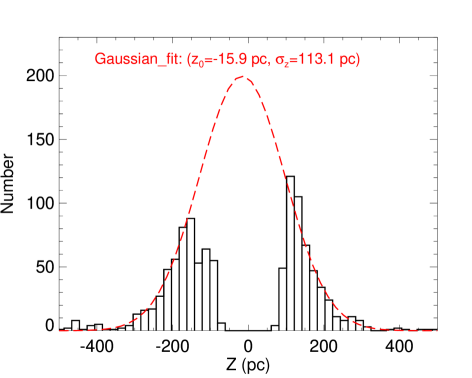
For the molecular gas far from the Galactic plane, Figure 8 displays the vertical distribution of the 1055 MCs, which can be fitted by a Gaussian function with pc and pc. The standard deviation of the vertical distribution is 113 pc (and thus the FWHM of 270 pc) for the gas layer traced by the ensemble of the high- MCs, which is roughly similar to the measurement from the CO emission in the thick molecular gas layer (Section 3.1).
Importantly, the excellent agreement of the vertical distribution of these discrete MCs with that of the thick CO disk emission proposed by Dame & Thaddeus (1994) confirms their claim that the high- emission they observed is not substantially contaminated by sidelobe pickup from the central disk. Therefore, our results based on the large-scale, high-resolution, and high-sensitivity data demonstrate convincingly that the thick molecular gas disk is indeed an important component in the inner Galaxy. The thick molecular disk is composed of many discrete MCs with small size and low mass (see below).
Figure 9 shows the properties of the MCs. Typically, these MCs have 1–4 K, with the median value of 2.1 K, indicating very faint CO emission (i.e., 4–10 pc-2 assuming a constant CO-to-H2 conversion factor) for these small MCs. The effective radii of these MCs are 08–16 (1–2 beam size), indicating that the MCs at the tangent are unresolved because of the spatial resolution limit of the data, i.e., 1–4 pc at distances of 5–8 kpc. We find that a truncated power-law function with a slope of =-1.74 (i.e., for the cloud’s mass range of ) can describe the mass distribution of the high- MCs, which is consistent to -1.7 observed for the MCs in the Milky Way (e.g., Roman-Duval et al., 2010; Heyer & Dame, 2015; Rice et al., 2016; Colombo et al., 2019). The velocity dispersion () of the high- MCs is roughly 0.8, leading to for the most of CO clouds.
Obviously, the lower limit of , radius, and surface density is related to (1) the limited sensitivity and spatial resolution of the current CO survey, and (2) the selection criterion of the MCs used in Section 3.3.1. We mention that some clouds with weak CO emission ( K) and/or smaller sizes (radius) are missed due to the observational limit of the MWISP survey. Therefore, a substantial amount of the fainter CO emission (e.g., K km s-1 or ) could probably be unveiled by higher-sensitivity CO surveys.
The cloud-cloud velocity dispersion () of these high- MCs can be estimated from the samples with . Obviously, the estimation of depends on the definition of the relation. By taking into account the slight variation of the tangent velocity, we find that the cloud-cloud dispersion varies from for to for with the bin samples in the region. The cloud-cloud velocity dispersion only changes a little with the variation of the selected tangent velocity. On the other hand, the estimated of these MCs is comparable to the measured cloud-cloud velocity dispersion of the total MC samples near the Galactic plane (see Section 3.4 and other works, e.g., Stark & Brand, 1989; Malhotra, 1994b).
Interestingly, the low of the high- MCs in the Milky Way is different from the finding that a potential thick gas disk may have a high velocity dispersion for galaxies (e.g., for the thick molecular gas disk with extended/diffuse CO emission; Caldú-Primo et al., 2013). As discussed in Krumholz et al. (2018), the high mass transport rates and star formation rates can lead to the high velocity dispersions of the gas in galaxies. Briefly, we summarized all of the physical properties for the high- MCs in Table 2.
As seen in Figure 10, the MCs are mainly concentrated in regions of (i.e., =3.1–4.1 kpc) and (i.e., =5.6–6.4 kpc). A smaller concentration is between the two peak distributions (i.e., see the or =4.3–5.0 kpc region in Figure 10). We suggest that the large-scale structures (i.e., the Norma arm, the Aquila Spur toward the tip of the Galactic bar, and the Carina-Sagittarius arm; see Figures 1 and 3; refer to Bland-Hawthorn & Gerhard, 2016; Reid et al., 2016) near the tangent points are probably responsible for the three peaks at the longitude distribution (or ) of the enhanced high- MCs. Interestingly, the scatter of is relatively larger in the region of (Figure 12), which indicates that the Galactic bar may have an important impact on the dynamics and distribution of the gas in the inner Galaxy.
We also find that the high- H i gas is abundant in the region of (Ford et al., 2010), although the vertical distribution of the high- H i clouds is much wider than that of the CO clouds (i.e., 300 pc pc vs. 100 pc pc in the 90% range). Figure 11 shows the comparison between the high- MWISP CO clouds and the GASS H i clouds in the range of l=[+171,+342] and b=[+51,51]. We note that some H i samples in Ford et al. (2010) are very likely related to our CO clouds, e.g., (1) the GASS H i cloud: (1872, 200, 126.1 ) versus the MWISP CO cloud: (18805, 1937, 131.27 ); (2) the GASS H i cloud: (1919, 206, 136.3 ) versus the MWISP CO cloud: (19213, 2134, 137.38 ); (3) the GASS H i cloud: (1961, 443, 138.0 ) versus the MWISP CO cloud: (19512, 4377, 137.84 ), etc. The spatial and kinematical relationships between the H i cloud and the CO cloud are worth exploring in more detail in future works by using the high-quality H i data (e.g., from the GALFA-HI survey; Peek et al., 2011, 2018) and MWISP CO data. Here we briefly discuss the possible origin of the high- MCs in Section 3.3.3.
In the region of (i.e., the region outside the of the thick CO disk), the molecular gas mass is about based on the discovered high- MCs by adopting =-15 pc and =120 pc (e.g., see Figure 8). The value is approximately of the total mass of the thick CO disk in the 5.1 kpc long red belt (see Figure 1; including an extrapolation of the component through the full Galactic disk by assuming a Gaussian distribution). Thus, the total mass of the thick CO disk in the belt region is about . Adopting a mean width of 0.5 kpc for the red belt (i.e., the mean path length along the line of sight for the belt; see the model in Lockman, 1984), we obtain an area of 2.55 kpc2 (i.e., 5.1 kpc length 0.5 kpc width) projected on the Galactic plane. The total midplane density of the thick disk is thus , leading to the volume density of (or ) in the discussed region by assuming the Gaussian distribution of exp. We mentioned that the estimated values are probably the lower limit due to the limited observational sensitivity and resolution of the MWISP survey (i.e., the missing molecular gas mass for the very faint CO emission and small clouds that are not involved in the calculation). In the region of 2–8.15 kpc, the molecular mass of the thick CO disk is thus , which is about 10% of the total molecular mass in the inner Galaxy (i.e., for the thin CO disk + the thick CO disk; this paper and Heyer & Dame, 2015).
3.3.3 Origin of the high- MCs
According to the vertical distribution of the high- molecular gas (Figure 8), we find that the identified MCs are mainly concentrated in the 100 pc 360 pc region. However, there is only a little amount of molecular gas traced by CO emission in the region of 360 pc (i.e., 32/1055 high- MCs). We thus suggest that these MCs with faint CO emission probably belong to the disk population. The spatial and velocity coincidence between some CO clouds and the corresponding H i clouds is very interesting. It indicates that considerable amounts of molecular gas appear to survive in the disk-halo transition region (or in the disk-halo zone close to the Galactic midplane; e.g., 100 pc 300 pc). The coexistence of molecular gas and the atomic gas in the disk-halo transition region needs to be further investigated based on the observational and theoretical studies.
Generally, the typical internal crossing time of these high- MCs is about 3 Myr assuming the typical radius of 3 pc and velocity dispersion of (Figure 9). This value is roughly an order of magnitude smaller than the dynamical timescale of the moving clouds from the Galactic midplane (i.e., t24 Myr, where is the cloud-cloud velocity dispersion from Section 3.4). It indicates that the MCs’ memory of their birthplace is lost, and any observed kinematical features from the line profile and spatial morphology probably represent the turbulence in the current local environment. Considering the prevalent turbulence in the ISM, the cloud will be destroyed quickly due to the Kelvin-Helmholtz and Rayleigh-Taylor instabilities (e.g, Myr in Iwasaki et al., 2019).
On the other hand, the high virial parameter of the clouds shows that the high- MCs are unstable unless they are confined by some external pressure. The low of and large of 260–300 pc for these high- MCs indicate that the gravitational force of the midplane is not balanced by the gas pressure, suggesting that the ensemble of the MCs is in general out of equilibrium. All of these results show that the high- MCs probably have short lifetimes less than several Myr (e.g., comparable to the typical internal crossing time). Indeed, if the MCs directly move from the Galactic plane to their current places, the moving velocity of the clouds should be an order of magnitude larger than that of the cloud-cloud dispersion velocity because of the short lifetime of these clouds (e.g., several Myr). Alternatively, some of the high- MCs are probably newborn clouds due to the rapid H2 formation in shock interaction regions (e.g., with the high ram pressure of , see Su et al., 2018). We suggest that these MCs are transitory. The high- molecular gas with faint CO emission is either dispersing or being assembled by some external dynamical processes (e.g., compression by shocks, cloud-cloud collision, and shear motions, etc).
Whatever the exact formation mechanism of the high- clouds, the energetic sources near the Galactic plane may play important roles in the origin of the disk-population gas (e.g., the stellar feedback from massive stellar winds and/or supernova explosions; see the Galactic fountain models in Shapiro & Field, 1976; Bregman, 1980; Houck & Bregman, 1990; Spitoni et al., 2008; Soler et al., 2020). Recently, di Teodoro et al. (2020) also found that the cold, dense, and high-velocity molecular gas survives in the Milky Way’s nuclear wind at 600–900 pc from the Galactic plane. Likewise, the interactions between the disk gas and the halo gas are probably common in the Milky Way and other galaxies due to energetic processes in the galactic plane (e.g., see the disk-halo scenario discussed in Lockman, 2002; Ford et al., 2008, 2010; Putman et al., 2012).
Finally, we summarize the thickness of the inner disk revealed by the different gas tracers in Table 3. The fact that the thickness of the thick disk traced by the CO gas (260–300 pc in this work) and the H i(C ii) gas (e.g., 250–270 pc for H i emission and 190–320 pc for C ii emission, Dickey & Lockman, 1990; Lockman & Gehman, 1991; Langer et al., 2014; Velusamy & Langer, 2014) is comparable may be a relevant hint to establishing a link between the formation/evolution of the high- MCs and various physical processes. Further studies will be helpful to clarify these issues through a combination of multiwavelength data, e.g., the kinematical connection between the CO clouds and the H i clouds, possible related IR features, and/or emission from other tracers like OH 18 cm, CH 3.3 GHz lines, and 158 m [C ii] lines, etc.
3.4 Cloud-to-cloud Velocity Dispersion near the Tangent Points and the Total Midplane Density
The H i and H2 gas in the inner Galaxy ( kpc) is concentrated toward the thin plane due to the gravitational potential of the matter in the Galactic disk. If the pressure from magnetic fields, cosmic rays, and the radiation field is ignored, the vertical distribution of the H2 gas is mainly determined by the total gravitating mass near the disk (i.e., stars, gas, and possible other unknown objects). Considering the balance between the turbulent pressure of the isothermal molecular gas and the gravitational force on the Galactic plane, we can obtain the formula of for the Gaussian distribution of the gas layer (e.g., see Malhotra, 1994b, 1995). Here, is the total density of the midplane mass, is the cloud-cloud velocity dispersion, and is the scale height of the thin CO layer. We ingore the scale height of the thick CO disk due to its limited contribution to the total molecular gas mass (i.e., 3% for the 120 pc molecular gas).
In principle, we can estimate the midplane mass density of the Galactic disk if and are obtained from observations. Figure 12 displays the distribution of for all MCs near the tangent points (i.e., MCs in the thin and thick disk with ). Here, is simply selected as (i.e., roughly three times of the scatter of , which is nearly constant for the tangent MCs in the longitude range) by taking into account the tangent MCs with somewhat lower . We note that the estimated value of is in the range of 2.7–7.9 (i.e., mean value of 4.9 and a scatter of 1.3), which is close to that of the high- MCs discussed in Section 3.3.2. The value is roughly consistent with other works based on different approaches (e.g., see Blitz et al., 1984; Clemens, 1985; Stark, 1984; Stark & Brand, 1989; Malhotra, 1994b).
Additionally, the distribution of seems to display a linear variation with a slope of kpc-1 between =2.2–6.4 kpc. It is interesting to note that the slope from the CO data is about one-half of the H i gas when the joint gravitational potential is considered (i.e., stars, H i gas, and H2 gas near the disk; see Narayan & Jog, 2002). The decrease of at larger may be explained by a lower star formation rate in the outer part of the inner disk if (i.e., the turbulence of the MCs) is regulated by the energy input via star-forming activities near the Galactic plane. On the other hand, however, it should be mentioned that the measured based on our CO data also displays considerable fluctuation in different (see Figure 12), which is probably related to the different localized environment. More quantitative studies are required to better understand these features.
Combining the measurements of – and – for MCs near the tangent points, we can obtain the distribution of the total mass density in the Galactic plane (i.e., – in Figure 13). The error of can be calculated from the fitting error of (Figure 7) and the assumed error of (Figure 12). We find that an exponential-disk model of can roughly fit the distribution of the total mass density for the =2.25–6.42 kpc region. Here, =1.28 pc-3 is the mass density at the Galactic center and kpc is the scale length of the disk. The midplane mass density at the Sun is estimated to be =0.10 pc-3, which agrees well with the Oort limit summarized in McKee et al. (2015). Because of the lower CO emission in the tangent points of (i.e., 3 kpc for the 3 kpc ring structure in Figure 2), we also fit the data in the =3.05–6.42 kpc region. The resultant fitting of – gives a similar result (see the blue line in Figure 13).
4 Summary
Based on the MWISP CO data, we have performed a study of the vertical distribution of the molecular gas near the tangent points in the range of – and 51. The main results are:
1. The terminal velocity of the molecular gas, which is comparable to other observations and theoretical models, is well determined from the new MWISP CO survey toward the inner Galaxy (Figure 2).
2. We use the CO emission near the terminal velocity to trace the molecular gas distribution at the tangent points, which can avoid the distance ambiguity within the solar circle. The high-quality CO data reveal two main molecular gas features near the tangent points, including large-scale bright CO emission in the Galactic midplane and discrete MCs with very weak emission in relatively high- regions (see Figure 3).
3. Based on the integrated CO intensity near the terminal velocity, we find that the model of two Gaussian components can be used to describe the vertical distribution of the molecular gas near the tangent points. The narrow one with a FWHM of 85 pc is the well-known thin molecular gas disk in the inner Galaxy, while another broad component with a FWHM of 260–300 pc probably represents the thick CO disk. For the thin CO disk, Figure 7 displays the systematic variation of the offset () and the scale height () of the molecular gas with respect to the Galactic longitude, which is consistent with previous studies (e.g., Malhotra, 1994b). For the thick CO disk, its thickness is about three times as wide as that of the well-known thin molecular gas layer, and the thickness of the thick molecular gas layer is very comparable in width to the central atomic gas layer (e.g., 250-270 pc in Dickey & Lockman, 1990; Lockman & Gehman, 1991).
4. For the thick CO disk, a total of 1055 high- MCs were identified at the tangent points in the first quadrant region of the MWISP survey. These MCs have a median radius of 2.5 pc, a median velocity dispersion of 0.8 , and a median peak temperature of 2.1 K. The mass surface brightness of the MCs is very low, i.e., a median value of 6.8 assuming a constant CO-to-H2 conversion factor of cm-2(K km s. The cloud-cloud velocity dispersion of the high- MCs is 4.4–5.6 , which is similar to the value of 4.9 for all MCs at the tangent points. The high virial parameter indicates that the high- MCs are probably short-lived objects. That is, the MCs of the new disk population are either dispersing or being assembled by some external dynamical processes. Alternatively, some of the high- MCs are probably newborn clouds in an environment of the high ram pressure. Our findings show that the thick CO disk is composed of many discrete MCs with small size and low mass (i.e., in the MC’s mass range of ).
5. Nearly 90% of these MCs are 100 pc from the plane. However, only 3% of MCs are in the pc region, suggesting that the high- molecular gas is the disk population. Including the emission of the CO layer through the whole Galactic plane, the total molecular gas mass of the thick CO disk is estimated to be in the range of 2–8.15 kpc, which is about 10% of the total molecular mass in the same region of the inner Galaxy. The surface density and midplane mass density of the thick molecular gas disk are and (or ), respectively.
6. The cloud-cloud velocity dispersion of all tangent MCs seems to be smaller at larger , leading to a slope of kpc-1 in the region of =2.2–6.4 kpc. This value is about one-half of the H i gas when the joint gravitational potential is considered (Narayan & Jog, 2002). The higher star formation rate at smaller is probably responsible for this feature.
7. Assuming the vertical equilibrium between the turbulent pressure of the molecular gas and the total gravitational force in the disk, we can use an exponential-disk model of to fit the distribution of the mass density in the Galactic midplane. The best-fit parameters are =3.2 kpc and =1.28 . The midplane mass density in the solar neighborhood is estimated to be 0.10 at 8.15 kpc, which agrees with the local mass density of 0.097 suggested by McKee et al. (2015).
References
- Benedettini et al. (2020) Benedettini, M., Molinari, S., Baldeschi, A., et al. 2020, A&A, 633, A147, doi: 10.1051/0004-6361/201936096
- Bland-Hawthorn & Gerhard (2016) Bland-Hawthorn, J., & Gerhard, O. 2016, ARA&A, 54, 529, doi: 10.1146/annurev-astro-081915-023441
- Blitz et al. (1984) Blitz, L., Magnani, L., & Mundy, L. 1984, ApJ, 282, L9, doi: 10.1086/184293
- Bolatto et al. (2013) Bolatto, A. D., Wolfire, M., & Leroy, A. K. 2013, ARA&A, 51, 207, doi: 10.1146/annurev-astro-082812-140944
- Bregman (1980) Bregman, J. N. 1980, ApJ, 236, 577, doi: 10.1086/157776
- Bronfman et al. (1988) Bronfman, L., Cohen, R. S., Alvarez, H., May, J., & Thaddeus, P. 1988, ApJ, 324, 248, doi: 10.1086/165892
- Caldú-Primo et al. (2013) Caldú-Primo, A., Schruba, A., Walter, F., et al. 2013, AJ, 146, 150, doi: 10.1088/0004-6256/146/6/150
- Clemens (1985) Clemens, D. P. 1985, ApJ, 295, 422, doi: 10.1086/163386
- Clemens et al. (1988) Clemens, D. P., Sanders, D. B., & Scoville, N. Z. 1988, ApJ, 327, 139, doi: 10.1086/166177
- Colombo et al. (2019) Colombo, D., Rosolowsky, E., Duarte-Cabral, A., et al. 2019, MNRAS, 483, 4291, doi: 10.1093/mnras/sty3283
- Combes (1991) Combes, F. 1991, ARA&A, 29, 195, doi: 10.1146/annurev.aa.29.090191.001211
- Dame et al. (2001) Dame, T. M., Hartmann, D., & Thaddeus, P. 2001, ApJ, 547, 792, doi: 10.1086/318388
- Dame & Thaddeus (1994) Dame, T. M., & Thaddeus, P. 1994, ApJ, 436, L173, doi: 10.1086/187660
- Dame & Thaddeus (2008) —. 2008, ApJ, 683, L143, doi: 10.1086/591669
- Dame & Thaddeus (2011) —. 2011, ApJ, 734, L24, doi: 10.1088/2041-8205/734/1/L24
- di Teodoro et al. (2020) di Teodoro, E. M., McClure-Griffiths, N. M., Lockman, F. J., & Armillotta, L. 2020, Nature, 584, 364. https://arxiv.org/abs/2008.09121
- Dickey & Lockman (1990) Dickey, J. M., & Lockman, F. J. 1990, ARA&A, 28, 215, doi: 10.1146/annurev.aa.28.090190.001243
- Du et al. (2017) Du, X., Xu, Y., Yang, J., & Sun, Y. 2017, ApJS, 229, 24, doi: 10.3847/1538-4365/aa5d9d
- Du et al. (2016) Du, X., Xu, Y., Yang, J., et al. 2016, ApJS, 224, 7, doi: 10.3847/0067-0049/224/1/7
- Eden et al. (2020) Eden, D. J., Moore, T. J. T., Currie, M. J., et al. 2020, MNRAS, 498, 5936, doi: 10.1093/mnras/staa2734
- Ford et al. (2010) Ford, H. A., Lockman, F. J., & McClure-Griffiths, N. M. 2010, ApJ, 722, 367, doi: 10.1088/0004-637X/722/1/367
- Ford et al. (2008) Ford, H. A., McClure-Griffiths, N. M., Lockman, F. J., et al. 2008, ApJ, 688, 290, doi: 10.1086/592188
- Garcia-Burillo et al. (1992) Garcia-Burillo, S., Guelin, M., Cernicharo, J., & Dahlem, M. 1992, A&A, 266, 21
- Heyer & Dame (2015) Heyer, M., & Dame, T. M. 2015, ARA&A, 53, 583, doi: 10.1146/annurev-astro-082214-122324
- Houck & Bregman (1990) Houck, J. C., & Bregman, J. N. 1990, ApJ, 352, 506, doi: 10.1086/168554
- Iwasaki et al. (2019) Iwasaki, K., Tomida, K., Inoue, T., & Inutsuka, S.-i. 2019, ApJ, 873, 6, doi: 10.3847/1538-4357/ab02ff
- Krumholz et al. (2018) Krumholz, M. R., Burkhart, B., Forbes, J. C., & Crocker, R. M. 2018, MNRAS, 477, 2716, doi: 10.1093/mnras/sty852
- Langer et al. (2014) Langer, W. D., Pineda, J. L., & Velusamy, T. 2014, A&A, 564, A101, doi: 10.1051/0004-6361/201323281
- Lockman (1984) Lockman, F. J. 1984, ApJ, 283, 90, doi: 10.1086/162277
- Lockman (2002) —. 2002, ApJ, 580, L47, doi: 10.1086/345495
- Lockman & Gehman (1991) Lockman, F. J., & Gehman, C. S. 1991, ApJ, 382, 182, doi: 10.1086/170706
- Malhotra (1994a) Malhotra, S. 1994a, ApJ, 437, 194, doi: 10.1086/174988
- Malhotra (1994b) —. 1994b, ApJ, 433, 687, doi: 10.1086/174677
- Malhotra (1995) —. 1995, ApJ, 448, 138, doi: 10.1086/175946
- McClure-Griffiths & Dickey (2016) McClure-Griffiths, N. M., & Dickey, J. M. 2016, ApJ, 831, 124, doi: 10.3847/0004-637X/831/2/124
- McKee et al. (2015) McKee, C. F., Parravano, A., & Hollenbach, D. J. 2015, ApJ, 814, 13, doi: 10.1088/0004-637X/814/1/13
- Nakanishi & Sofue (2006) Nakanishi, H., & Sofue, Y. 2006, PASJ, 58, 847, doi: 10.1093/pasj/58.5.847
- Narayan & Jog (2002) Narayan, C. A., & Jog, C. J. 2002, A&A, 394, 89, doi: 10.1051/0004-6361:20021128
- Peek et al. (2011) Peek, J. E. G., Heiles, C., Douglas, K. A., et al. 2011, ApJS, 194, 20, doi: 10.1088/0067-0049/194/2/20
- Peek et al. (2018) Peek, J. E. G., Babler, B. L., Zheng, Y., et al. 2018, ApJS, 234, 2, doi: 10.3847/1538-4365/aa91d3
- Pety (2005) Pety, J. 2005, in SF2A-2005: Semaine de l’Astrophysique Francaise, ed. F. Casoli, T. Contini, J. M. Hameury, & L. Pagani, (Les Ulis: EDP), 721
- Pety et al. (2013) Pety, J., Schinnerer, E., Leroy, A. K., et al. 2013, ApJ, 779, 43, doi: 10.1088/0004-637X/779/1/43
- Putman et al. (2012) Putman, M. E., Peek, J. E. G., & Joung, M. R. 2012, ARA&A, 50, 491, doi: 10.1146/annurev-astro-081811-125612
- Reid et al. (2016) Reid, M. J., Dame, T. M., Menten, K. M., & Brunthaler, A. 2016, ApJ, 823, 77, doi: 10.3847/0004-637X/823/2/77
- Reid et al. (2019) Reid, M. J., Menten, K. M., Brunthaler, A., et al. 2019, ApJ, 885, 131, doi: 10.3847/1538-4357/ab4a11
- Rice et al. (2016) Rice, T. S., Goodman, A. A., Bergin, E. A., Beaumont, C., & Dame, T. M. 2016, ApJ, 822, 52, doi: 10.3847/0004-637X/822/1/52
- Rigby et al. (2016) Rigby, A. J., Moore, T. J. T., Plume, R., et al. 2016, MNRAS, 456, 2885, doi: 10.1093/mnras/stv2808
- Roman-Duval et al. (2010) Roman-Duval, J., Jackson, J. M., Heyer, M., Rathborne, J., & Simon, R. 2010, ApJ, 723, 492, doi: 10.1088/0004-637X/723/1/492
- Sanders et al. (1984) Sanders, D. B., Solomon, P. M., & Scoville, N. Z. 1984, ApJ, 276, 182, doi: 10.1086/161602
- Schuller et al. (2017) Schuller, F., Csengeri, T., Urquhart, J. S., et al. 2017, A&A, 601, A124, doi: 10.1051/0004-6361/201628933
- Schuller et al. (2021) Schuller, F., Urquhart, J. S., Csengeri, T., et al. 2021, MNRAS, 500, 3064, doi: 10.1093/mnras/staa2369
- Shan et al. (2012) Shan, W., Yang, J., Shi, S., et al. 2012, ITTST, 2, 593, doi: 10.1109/TTHZ.2012.2213818
- Shapiro & Field (1976) Shapiro, P. R., & Field, G. B. 1976, ApJ, 205, 762, doi: 10.1086/154332
- Sofue et al. (2019) Sofue, Y., Kohno, M., Torii, K., et al. 2019, PASJ, 71, S1, doi: 10.1093/pasj/psy094
- Soler et al. (2020) Soler, J. D., Beuther, H., Syed, J., et al. 2020, A&A, 642, A163, doi: 10.1051/0004-6361/202038882
- Spitoni et al. (2008) Spitoni, E., Recchi, S., & Matteucci, F. 2008, A&A, 484, 743, doi: 10.1051/0004-6361:200809403
- Stark (1984) Stark, A. A. 1984, ApJ, 281, 624, doi: 10.1086/162137
- Stark & Brand (1989) Stark, A. A., & Brand, J. 1989, ApJ, 339, 763, doi: 10.1086/167334
- Su et al. (2016) Su, Y., Sun, Y., Li, C., et al. 2016, ApJ, 828, 59, doi: 10.3847/0004-637X/828/1/59
- Su et al. (2018) Su, Y., Zhou, X., Yang, J., et al. 2018, ApJ, 863, 103, doi: 10.3847/1538-4357/aad04e
- Su et al. (2019) Su, Y., Yang, J., Zhang, S., et al. 2019, ApJS, 240, 9, doi: 10.3847/1538-4365/aaf1c8
- Sun et al. (2018) Sun, J. X., Lu, D. R., Yang, J., et al. 2018, AcASn, 59, 3
- Sun et al. (2017) Sun, Y., Su, Y., Zhang, S.-B., et al. 2017, ApJS, 230, 17, doi: 10.3847/1538-4365/aa63ea
- Sun et al. (2015) Sun, Y., Xu, Y., Yang, J., et al. 2015, ApJ, 798, L27, doi: 10.1088/2041-8205/798/2/L27
- Sun et al. (2020) Sun, Y., Yang, J., Xu, Y., et al. 2020, ApJS, 246, 7, doi: 10.3847/1538-4365/ab5b97
- Torii et al. (2019) Torii, K., Fujita, S., Nishimura, A., et al. 2019, PASJ, 71, S2, doi: 10.1093/pasj/psz033
- Vallée (2014) Vallée, J. P. 2014, ApJS, 215, 1, doi: 10.1088/0067-0049/215/1/1
- Velusamy & Langer (2014) Velusamy, T., & Langer, W. D. 2014, A&A, 572, A45, doi: 10.1051/0004-6361/201424350
- Yan et al. (2020) Yan, Q.-Z., Yang, J., Su, Y., Sun, Y., & Wang, C. 2020, ApJ, 898, 80, doi: 10.3847/1538-4357/ab9f9c


|
|
|
|
|
|
|
|
|
|
|
|||||||||||||||||||||||||||||||
|---|---|---|---|---|---|---|---|---|---|---|---|---|---|---|---|---|---|---|---|---|---|---|---|---|---|---|---|---|---|---|---|---|---|---|---|---|---|---|---|---|---|
| 1 | 16.103 | 0.896 | 143.16 | 2.07 | 1.84 | 10.75 | 7.8 | 122.5 | 690 | 31.5 | |||||||||||||||||||||||||||||||
| 2 | 16.278 | 0.976 | 137.99 | 1.00 | 1.29 | 2.50 | 7.8 | 133.2 | 100 | 24.2 | |||||||||||||||||||||||||||||||
| 3 | 16.436 | -0.770 | 128.18 | 0.85 | 1.97 | 5.00 | 7.8 | -105.0 | 160 | 15.4 | |||||||||||||||||||||||||||||||
| 4 | 16.498 | 0.809 | 130.07 | 1.31 | 2.60 | 14.25 | 7.8 | 110.4 | 620 | 15.9 | |||||||||||||||||||||||||||||||
| 5 | 16.526 | 0.929 | 139.87 | 3.27 | 2.54 | 15.75 | 7.8 | 126.7 | 1160 | 56.4 | |||||||||||||||||||||||||||||||
| 6 | 16.768 | -0.600 | 128.00 | 1.37 | 3.30 | 31.50 | 7.8 | -81.8 | 1700 | 9.5 | |||||||||||||||||||||||||||||||
| 7 | 16.801 | -1.173 | 128.58 | 0.77 | 1.70 | 6.50 | 7.8 | -159.8 | 220 | 10.5 |
Note. — a The error of the estimated distance is about 2%–20% from assuming that the MCs are located near tangent points with a velocity uncertainty of along the line of sight (e.g., refer to the A5 model in Reid et al., 2019). b The MC’s virial parameter estimated from the definition of (see Section 3.3.1).
| Median | Mean | ||||||||||||||||||||||||
|---|---|---|---|---|---|---|---|---|---|---|---|---|---|---|---|---|---|---|---|---|---|---|---|---|---|
|
|
|
|
|
|
|
|
|
|||||||||||||||||
| 2.1 | 2.5 | 0.8 | 136.3 | 6.8 | 12.9 | 4.4–5.6 | 280 | -1.74 | |||||||||||||||||
Note. — a The properties of the molecular gas indicate that the high- MCs belong to a new disk population that was not discovered by previous CO observations due to the low sensitivity, low resolution, and/or limited latitude coverage. b is the virial parameter of the MCs (see the text). c is the spectral index of the mass distribution of the high- MCs with the form in the MC’s mass range of .
| Tracer | FWHMa | Referencesb | Comments |
|---|---|---|---|
| CO | 85 pc | 1,2 | The well-known thin molecular gas disk |
| 280 pc | 1 | The thick disk is composed of many discrete MCs with small size and low mass | |
| C ii | 120 pc | 3 | C ii with bright CO emission as the dense H2 gas (the overestimated thin CO disk) |
| 190 pc | 3 | Bright diffuse C ii emission as the CO-faint diffuse H2 gas | |
| 320 pc | 3 | Faint diffuse C ii emission as the diffuse H i and WIM gas | |
| H i | 230 pc | 4,5 | The narrow Gaussian component for the cold neutral medium |
| 540 pc | 4,5 | The broad Gaussian component for the warm neutral medium | |
| 1300-1600 pc | 5,6 | The exponential component for the warm neutral medium (the disk-halo gas) |