MolGrow: A Graph Normalizing Flow for Hierarchical Molecular Generation
Abstract
We propose a hierarchical normalizing flow model for generating molecular graphs. The model produces new molecular structures from a single-node graph by recursively splitting every node into two. All operations are invertible and can be used as plug-and-play modules. The hierarchical nature of the latent codes allows for precise changes in the resulting graph: perturbations in the top layer cause global structural changes, while perturbations in the consequent layers change the resulting molecule marginally. The proposed model outperforms existing generative graph models on the distribution learning task. We also show successful experiments on global and constrained optimization of chemical properties using latent codes of the model.
Introduction
Drug discovery is a challenging multidisciplinary task that combines domain knowledge in chemistry, biology, and computational science. Recent works demonstrated successful applications of machine learning to the drug development process, including synthesis planning (Segler, Preuss, and Waller 2018), protein folding (Senior et al. 2020), and hit discovery (Merk et al. 2018; Zhavoronkov et al. 2019; Kadurin et al. 2016). Advances in generative models enabled applications of machine learning to drug discovery, such as distribution learning and molecular property optimization. Distribution learning models train on a large dataset to produce novel compounds (Polykovskiy et al. 2020); property optimization models search the chemical space for molecules with desirable properties (Brown et al. 2019). Often researchers combine these tasks: they first train a distribution learning model and then use its latent codes to optimize molecular properties (Gómez-Bombarelli et al. 2018). For such models, proper latent codes are crucial for molecular space navigation.
We propose a new graph generative model—MolGrow. Starting with a single node, it iteratively splits every node into two. Our model is invertible and maps molecular structures onto a fixed-size hierarchical manifold. Top levels of the manifold define global structure, while the bottom levels influence local features.
Our contributions are three-fold:
-
•
We propose a hierarchical normalizing flow model for generating molecular graphs. The model gradually increases graph size during sampling, starting with a single node;
-
•
We propose a fragment-oriented atom ordering that improves our model over commonly used breadth-first search ordering;
-
•
We apply our model to distribution learning and property optimization tasks. We report distribution learning metrics (Fréchet ChemNet distance and fragment distribution) for graph generative models besides providing standard uniqueness and validity measures.
Background: Normalizing Flows
Normalizing flows are generative models that transform a prior distribution into a target distribution by composing invertible functions :
| (1) | |||
| (2) |
We call Equation 1 a forward path, and Equation 2 an inverse path. The prior distribution is often a standard multivariate normal distribution . Such models are trained by maximizing training set log-likelihood using the change of variables formula:
| (3) |
where , . To efficiently train the model and sample from it, inverse transformations and Jacobian determinants should be tractable and computationally efficient. In this work, we consider three types of layers: invertible linear layer, actnorm, and real-valued non-volume preserving transformation (RealNVP) (Dinh, Sohl-Dickstein, and Bengio 2017). We define these layers below for arbitrary -dimensional vectors, and extend these layers for graph-structured data in the next section.
We consider an invertible linear layer parameterization by Hoogeboom, Van Den Berg, and Welling (2019) that uses QR decomposition of a weight matrix: , where is an orthogonal matrix (), and is an upper triangular matrix with ones on the main diagonal. We use Householder reflections to parameterize Q:
| (4) |
where are learnable column-vectors. The Jacobian determinant of a linear layer is . There is an alternative way to formulate a linear layer with LU decomposition (Kingma and Dhariwal 2018). However, in our experiments, QR decomposition showed more numerically stable results.
Actnorm layer (Kingma and Dhariwal 2018) is a linear layer with a diagonal weight matrix: , where is an element-wise multiplication. Vectors and are initialized so that the output activations from this layer have zero mean and unit variance at the beginning of training. We use the first training batch for initialization. The Jacobian determinant of this layer is .
RealNVP layer (Dinh, Sohl-Dickstein, and Bengio 2017) is a nonlinear invertible transformation. Consider a vector of length with first half of the components denoted as , and the second half as . Then, RealNVP and its inverse transformations are:
| (5) | |||
| (6) |
Functions and do not have to be invertible, and usually take form of a neural network. The Jacobian determinant of the RealNVP layer is . We sequentially apply two RealNVP layers to transform both components of . We also use permutation layer that deterministically shuffles input dimensions before RealNVP—this is equivalent to randomly splitting data into and parts.
MolGrow (Molecular Graph Flow)
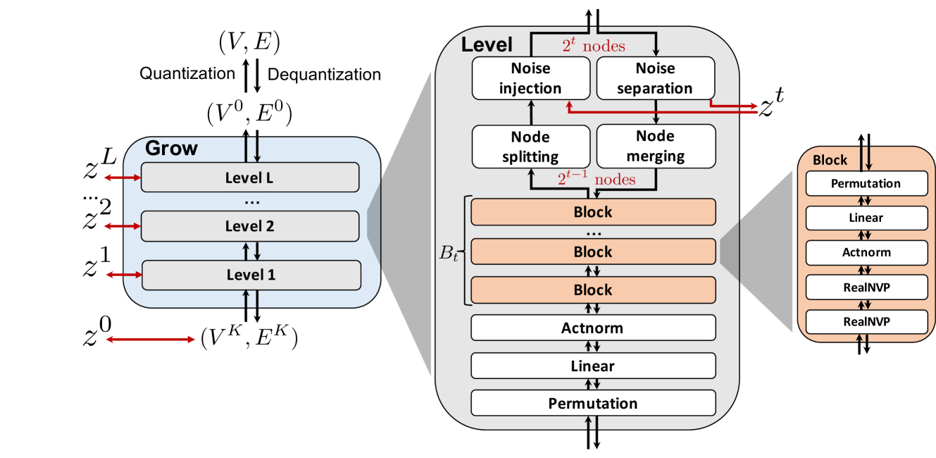
In this section, we present our generative model—MolGrow. MolGrow is a hierarchical normalizing flow model (Figure 1): it produces new molecular graphs from a single-node graph by recursively dividing every node into two. The final graph has nodes, where is a number of node-splitting layers in the model. To generate graphs with fewer nodes, we add special padding atoms. We choose to be large enough to fit any graph from the training dataset.
We represent a graph with node attribute matrix and edge attribute tensor , where and are feature dimensions. For the input data, defines atom type and charge, defines edge type. Since molecular graphs are non-oriented, we preserve the symmetry constraint on all intermediate layers: .
We illustrate MolGrow’s architecture in Figure 1. MolGrow consists of invertible levels, each level has its own latent code with a Gaussian prior. On a forward path, each level extracts the latent code and halves the graph size by merging node pairs. On the inverse path, each level does the opposite: it splits each node into two and adds additional noise. The final output on the forward path is a single-node graph graph and latent codes from each level: . We call a top level latent code.
Dequantization
To avoid fitting discrete graphs into a continuous density model, we dequantize the data using a uniform noise (Kingma and Dhariwal 2018):
| (7) | |||
| (8) |
Elements of and are independent samples from a uniform distribution . Such dequantization is invertible for —original data can be reconstructed by rounding down the elements of and . We dequantize the data for each training batch independently and train the model on . Dequantizated graph is a complete graph.
Node merging and splitting
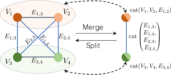
We use node merging and splitting operations to control the graph size. These operations are inverse of each other, and both operate by rearranging node and edge features. Consider a graph with nodes. Node merging operation joins nodes and into a single node by concatenating their features and features of the edge between them. We concatenate edge features connecting the merged nodes:
| (9) | |||
| (10) |
Node splitting is the inverse of node merging layer: it slices features into original components. See an example in Figure 2.
Noise separation and injection
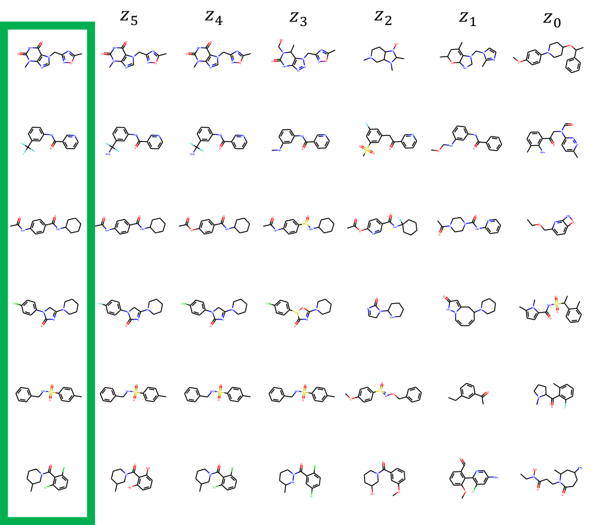
MolGrow produces a latent vector for each level. We derive the latent codes by separating half of the node and edge features before node merging and impose Gaussian prior on these latent codes. During generation, we sample the latent code from the prior and concatenate it with node and edge features. As we show in the experiments, latent codes on different levels affect the generated structure differently. Latent codes from smaller intermediate graphs (top level) influence global structure, while bottom level features define local structure.
Block architecture
The basic building block in MolGrow (denoted block in Figure 1) consists of five layers. The first three layers (permutation, linear, and actnorm) serve as convolutions. Each layer contains two transformations: one transforms every node and the other transforms every edge. The number of linear layer’s Housholder reflections in matrix is smaller than the dimension of . Hence, a combination of linear and permutation layers is not equivalent to a single linear layer.
The final two layers of the block are RealNVP layers. RealNVP layer splits its input graph with nodes into and along features dimension. We transform by projecting node and edge features onto a low-dimensional manifold and applying attention on complete graph edges (CAGE) architecture (Algorithm 1). We compute the final output of RealNVP layer by applying fully-connected neural networks , , , and to each node and edge independently:
| (11) | |||
| (12) | |||
| (13) | |||
| (14) | |||
| (15) |
Similar to other attentive graph convolutions (Veličković et al. 2017; Guo, Zhang, and Lu 2019), CAGE architecture uses a multi-head attention (Vaswani et al. 2017). It also uses gated recurrent unit update function to stabilize training (Parisotto et al. 2020). Positional encoding in CAGE consists of two parts. First dimensions are standard sinusoidal positional encoding (Vaswani et al. 2017):
| (16) | |||
| (17) |
The last components of contain a binary code of . We add multiple blocks before the first and after the last level in the full architecture.
Layout and padding
Similar to the previous works (Shi et al. 2020; You et al. 2018b), we achieved better results when learning on a fixed atom ordering, instead of learning a distribution over all permutations. Previous works used breadth-first search (BFS) atom ordering, since it avoids long-range dependencies. However, BFS does not incorporate the knowledge of common fragments and can mix their atoms (Figure 3a). We propose a new atom ordering to incorporate prior knowledge about frequent fragments. Our ordering better organizes the latent space and simplifies generation.
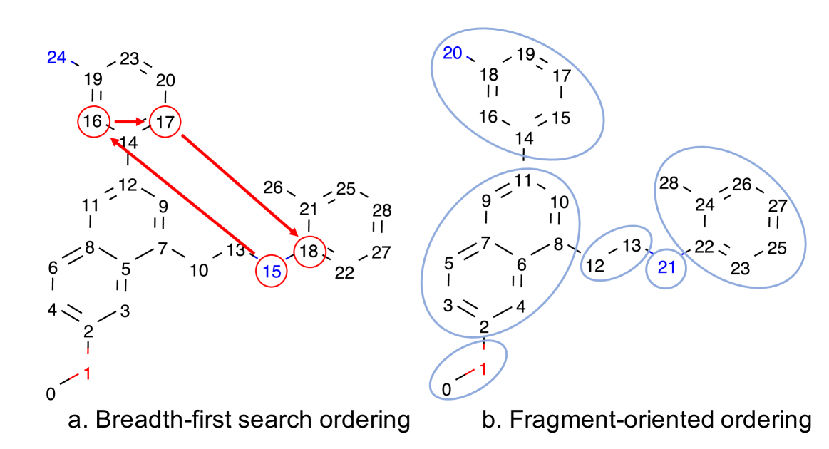
We break the molecule into fragments by removing BRICS (Degen et al. 2008) bonds and bonds connecting rings, linkers, and decorations in the Bemis-Murcko scaffold (Bemis and Murcko 1996). We then enumerate the fragments and atoms in each fragment using BFS ordering (Figure 3b). We recursively choose padding positions, minimizing the number of edges after node merging layers (Algorithm 2).
| Method | FCD/Test | Frag/Test | Unique@10k | Novelty |
|---|---|---|---|---|
| Graph-based models | ||||
| MolecularRNN (Popova et al. 2019) | 23.13 | 0.56 | 98.6% | 99.9% |
| GraphVAE (Simonovsky and Komodakis 2018) | 49.39 | 0.0 | 5% | 100% |
| GraphNVP (Madhawa et al. 2019) | 29.95 | 0.62 | 99.7 % | 99.9% |
| GraphAF (BFS) (Shi et al. 2020) | 21.84 | 0.651 | 97% | 99.9% |
| MoFlow (Zang and Wang 2020) | 28.05 | 0.685 | 100% | 99.99% |
| Proposed model | ||||
| MolGrow (fragment-oriented) | % | % | ||
| MolGrow (BFS) | % | % | ||
| MolGrow (BFS on fragments) | % | % | ||
| MolGrow (random permutation) | % | % | ||
| MolGrow (GAT instead of CAGE) | % | % | ||
| MolGrow (No positional embedding) | % | % | ||
| SMILES and fragment-based models | ||||
| CharRNN (from MOSES benchmark) | 0.073 | 0.9998 | 99.73% | 84.19% |
| VAE (from MOSES benchmark) | 0.099 | 0.9994 | 99.84% | 69.49% |
| JTN-VAE (from MOSES benchmark) | 0.422 | 0.9962 | 100% | 91.53% |
Related work
Many well-known generative models work out of the box for molecular generation task. By representing molecules as strings, one can apply any sequence generation model: language models (Segler et al. 2018), variational autoencoders (Gómez-Bombarelli et al. 2018), and generative adversarial networks (Sanchez-Lengeling et al. 2017). Molecular graphs satisfy a formal set of rules: all atoms must have a proper valency, and a graph must have only one component. These constraints can be learned implicitly from the data or explicitly by specifying grammar rules (Kusner, Paige, and Hernández-Lobato 2017; O’Boyle and Dalke 2018; Krenn et al. 2019).
Multiple generative models for molecular graphs were proposed. Graph recurrent neural network (GraphRNN) (You et al. 2018b) and molecular recurrent neural network (MolecularRNN) (Popova et al. 2019) use node and edge generators: node generator sequentially produces nodes; edge generator sequentially predicts edge types for all the previous nodes from the hidden states of a node generator. Molecular generative adversarial network (MolGAN) (De Cao and Kipf 2018) trains a critic on generated graphs and passes the gradient to the generator using deep deterministic policy gradient (Lillicrap et al. 2015). Graph variational autoencoder (GraphVAE) (Simonovsky and Komodakis 2018) encodes and decodes molecules using edge-conditioned graph convolutions (Simonovsky and Komodakis 2017). Graph autoregressive flow (GraphAF) (Shi et al. 2020) iteratively produces nodes and edges; discrete one-hot vectors are dequantized, and tokens are decoded using argmax. The most similar work to ours is a graph non-volume preserving transformation (GraphNVP) (Madhawa et al. 2019) model. GraphNVP generation is not autoregressive: the model produces a dequantized adjacency matrix using normalizing flow, turns it into a discrete set of edges by computing argmax, and obtains atom types using a normalizing flow. MoFlow (Zang and Wang 2020) exploits a two-stage graph generation process similar to GraphNVP: first, it generates an adjacency matrix with Glow architecture and then recovers node attributes with additional coupling layers. Unlike GraphNVP and MoFlow, we generate the graph hierarchically and inject noise on multiple levels. We also produce nodes and edges simultaneously. Tran et al. (2019) model discrete data directly with straight-through gradient estimators. Application of such model to graph structured data is yet to be explored.
All graph generative models mentioned above are not permutation invariant, and most of these models employ a fixed atom order. GraphVAE aligns generated and target graphs using Hungarian algorithm, but has high computational complexity. Vinyals, Bengio, and Kudlur (2016) report that order matters in set to set transformation problems with specific orderings giving better results. Most models learn on a breadth-first search (BFS) atom ordering (You et al. 2018b). In BFS, new nodes are connected only to the nodes produced on the current or previous BFS layers, avoiding long range dependencies. Alternatively, graph generative models could use a canonical depth-first search (DFS) order (Weininger, Weininger, and Weininger 1989). Note that unlike graph-based generators, string-based generators seem to improve from augmenting atom orders (Bjerrum 2017).
Several works studied fragment-based molecular generation. Jin, Barzilay, and Jaakkola (2018) replace molecular fragments with nodes to form a junction tree. They then produce molecules by sampling a junction tree and then expanding it into a full molecule. The authors expanded this approach to incorporate larger fragments as tokens (motifs) (Jin, Barzilay, and Jaakkola 2020).
Experiments
We consider three problems: distribution learning, global molecular property optimization and constrained optimization. For all the experiments, we provide model and optimization hyperparameters in supplementary material A; the source code for reproducing all the experiments is provided in supplementary materials. We consider hydrogen-depleted graphs, since hydrogens can be deduced from atom valence.
Distribution learning
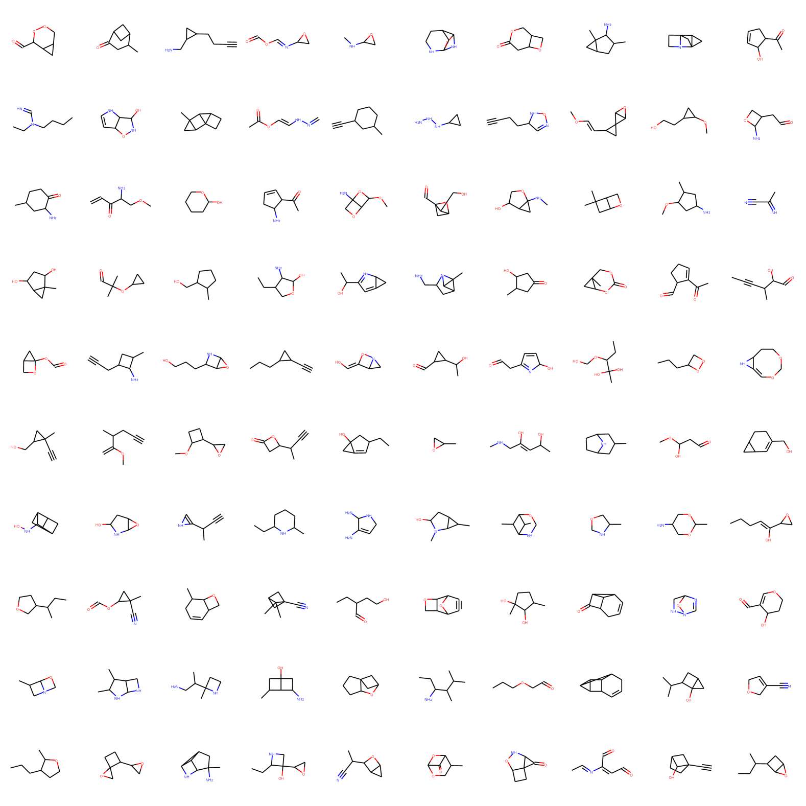
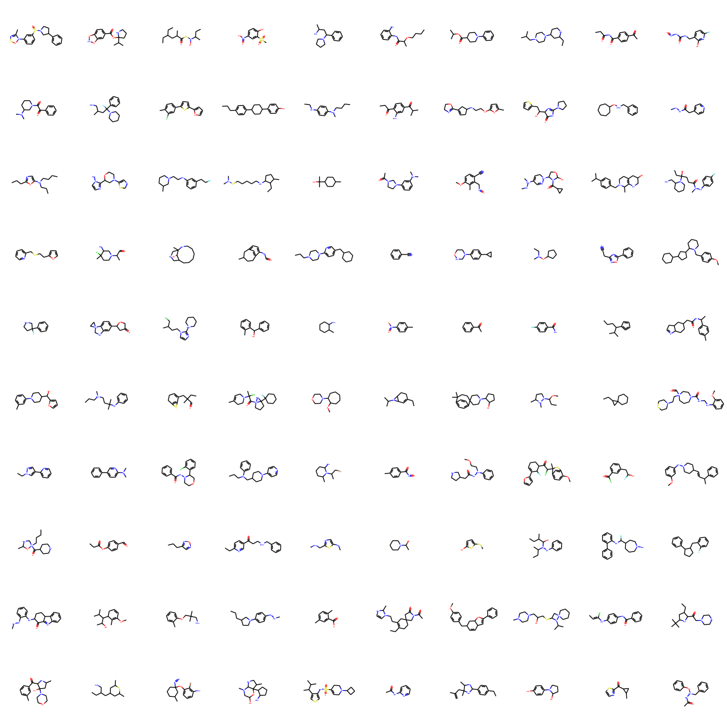
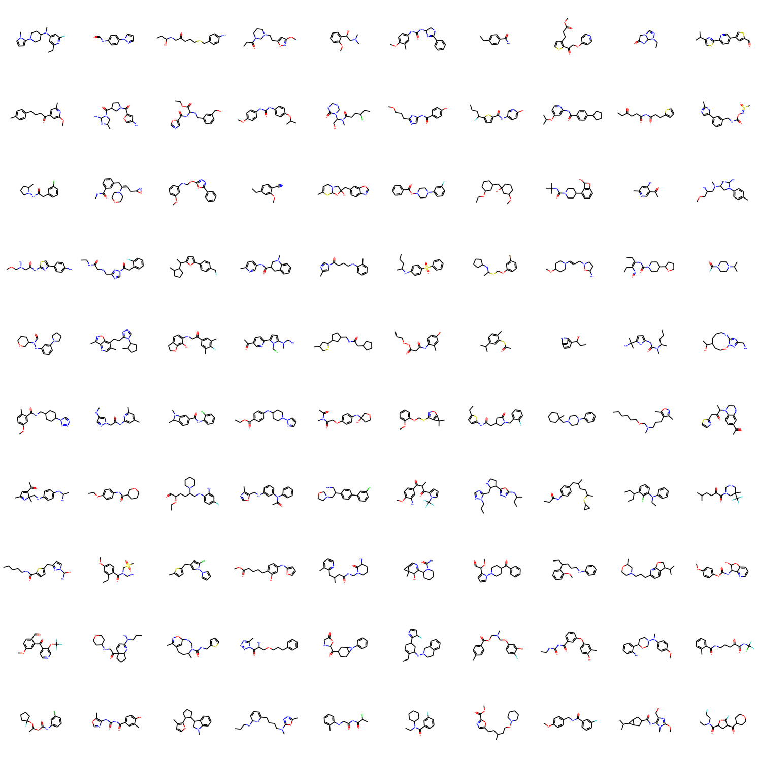
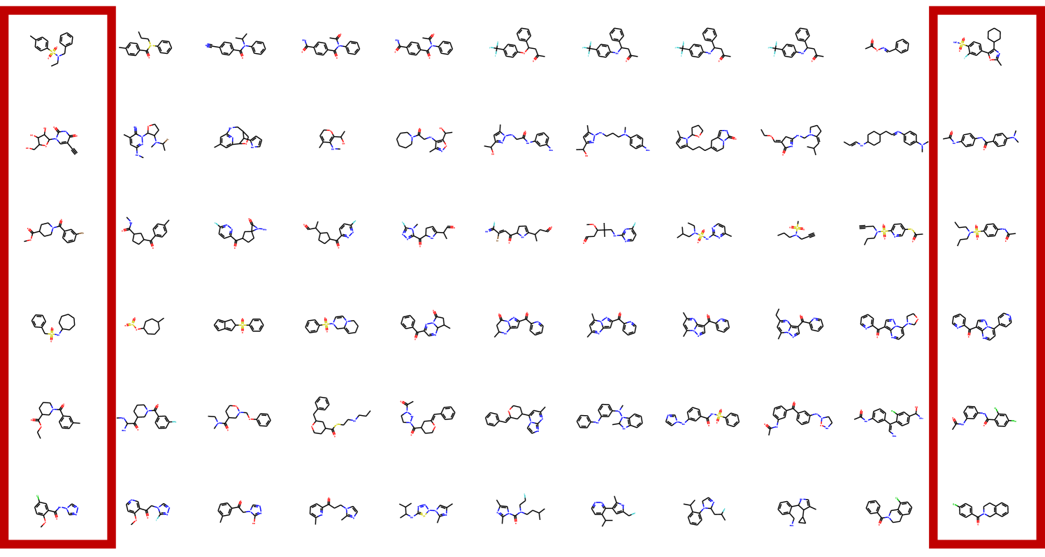
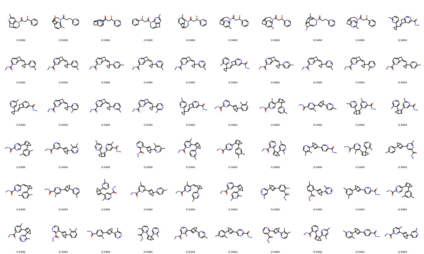
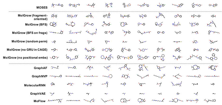
In distribution learning task, we assess how well models capture the data distribution. We compare generated and a test sets using Fréchet ChemNet distance (FCD/Test) (Preuer et al. 2018). FCD/Test is a Wasserstein-1 distance between Gaussian approximations of ChemNet’s penultimate layer activations. We also computed cosine similarity between fragment frequency vectors in the generated and test sets. We report the results on MOSES (Polykovskiy et al. 2020) dataset in Table 1. MolGrow outperforms previous node-level graph generators by a large margin. Note that SMILES-based generators (CharRNN and VAE) and fragment-level generator (JTN-VAE) outperform all node-level graph models. We hypothesize that such representations impose strong prior on the generated structures. We provide samples from graph-based models in Figure 4. Note that baseline models tend to produce macrocycles which were not present in the training set; molecules produced with GraphNVP contain too few rings. Ablation study demonstrates the advantage of fragment-oriented ordering and CAGE over standard graph attention network GAT (Veličković et al. 2017). We provide the results on QM9 (Ramakrishnan et al. 2014) and ZINC250k (Kusner, Paige, and Hernández-Lobato 2017) datasets in supplementary material B. In Figure 6 of Supplementary materials, we show how resampling different latent codes affect the generated structure.
Global optimization
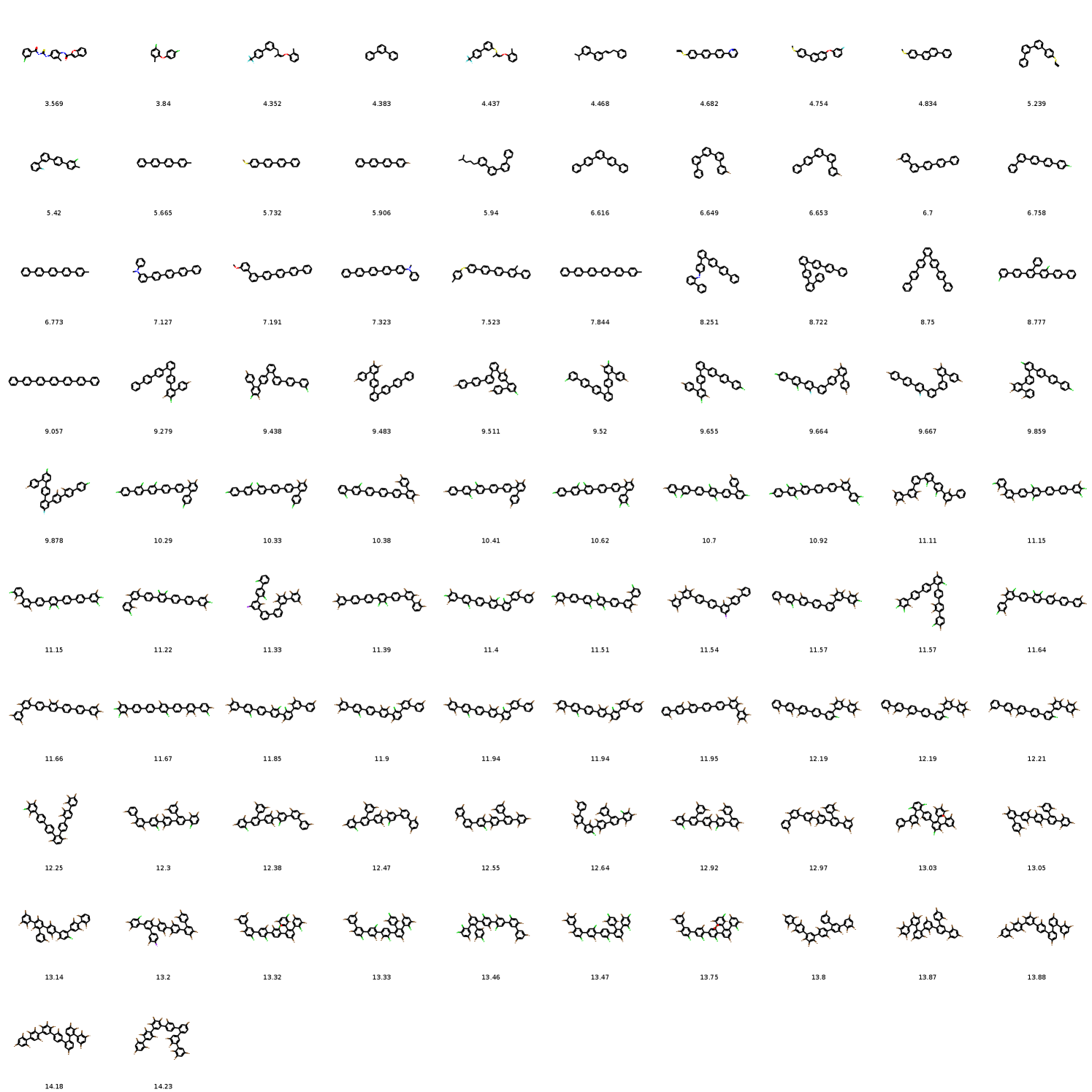
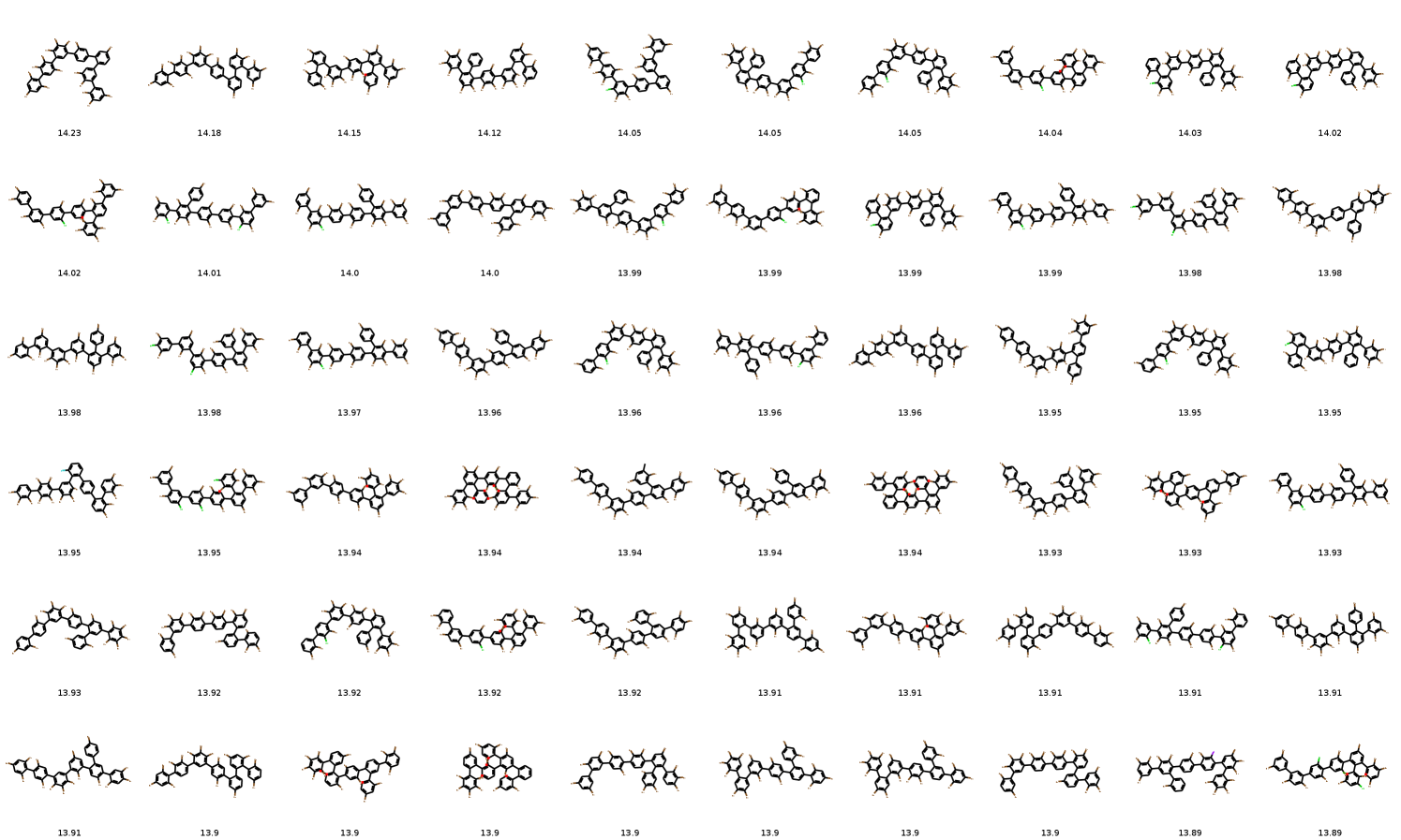
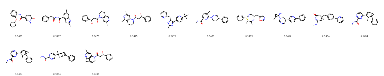
The goal of a global optimization task is to produce new molecules that maximize a given chemical property. Similar to the previous works, we selected two commonly used properties: penalized octanol-water partition coefficient (penalized logP) (Kusner, Paige, and Hernández-Lobato 2017) and quantitative estimation of drug-likeness (QED) (Gómez-Bombarelli et al. 2018). We considered genetic and predictor-guided optimization strategies.
For genetic optimization, we start by sampling random molecules from ZINC250k dataset and computing their latent codes. Then we hierarchically optimize latent codes for iterations. At each iteration we generate a new population using crossing-over and mutation and keep molecules with the highest reward. In crossing-over, we randomly permute all molecules in the population to form pairs. For each pair, we uniformly sample latent codes from spherical linear interpolation (Slerp) trajectory (White 2016) and reconstruct the resulting molecule. We mutate one level’s latent code at each iteration. Starting with a top level, we resample of the components from a Gaussian distribution. For genetic optimization, we compare different mutation and crossing-over strategies, including top level optimization with fixed bottom layers and vice versa.
In predictor-guided optimization, we followed the approach proposed by Jin, Barzilay, and Jaakkola (2018): we fine-tuned the pre-trained model jointly with a penalized logP predictor from the high-level latent codes for one epoch (MAE= for penalized logP, MAE= for QED). We randomly sampled molecules from a prior distribution and took constrained gradient ascent steps along the predictor’s gradient to modify the high-level latent codes; we resample low-level latent codes from the prior. We decrease the learning rate after each iteration and keep the best reconstructed molecule that falls into the constrained region. Intuitively, the gradient ascent over high-level latent codes guides the search towards better global structure, while low-level latent codes produce a diverse set of molecules with the same global structure and similar predicted values.
We report the scores of the best molecules found during optimization in Table 2 and provide optimization trajectories in supplementary information C.
| Method | Penalized logP | QED | ||||
|---|---|---|---|---|---|---|
| 1st | 2nd | 3rd | 1st | 2nd | 3rd | |
| ZINC250k | 4.52 | 4.30 | 4.23 | 0.948 | 0.948 | 0.948 |
| Graph-based models | ||||||
| GCPN (You et al. 2018a) | 7.98 | 7.85 | 7.80 | 0.948 | 0.947 | 0.946 |
| MolecularRNN (Popova et al. 2019) | 8.63 | 6.08 | 4.73 | 0.844 | 0.796 | 0.736 |
| GraphNVP (Madhawa et al. 2019) | - | - | - | 0.833 | 0.723 | 0.706 |
| GraphAF (Shi et al. 2020) | 12.23 | 11.29 | 11.05 | 0.948 | 0.948 | 0.948 |
| MoFlow (Zang and Wang 2020) | - | - | - | 0.948 | 0.948 | 0.948 |
| Proposed model | ||||||
| MolGrow (GE) | ||||||
| MolGrow (GE, Top only) | ||||||
| MolGrow (GE, Bottom only) | ||||||
| MolGrow (predictor-guided optimization) | ||||||
| MolGrow (REINFORCE) | ||||||
| SMILES and fragment-based models | ||||||
| DD-VAE (Polykovskiy and Vetrov 2020) | 5.86 | 5.77 | 5.64 | - | - | - |
| Grammar VAE (Kusner, Paige, and Hernández-Lobato 2017) | 2.94 | 2.88 | 2.80 | - | - | - |
| SD-VAE (Dai et al. 2018) | 4.04 | 3.50 | 2.96 | - | - | - |
| JT-VAE (Jin, Barzilay, and Jaakkola 2018) | 5.30 | 4.93 | 4.49 | 0.948 | 0.947 | 0.947 |
Constrained optimization
In this section, we apply MolGrow to constrained molecular optimization. In this task, we optimize a chemical property in proximity of the initial molecule. Following the previous works (Jin, Barzilay, and Jaakkola 2018; You et al. 2018a), we selected molecules with the lowest penalized octanol-water partition coefficient (logP) and constrain minimum Tanimoto similarity between Morgan fingerprints (Rogers and Hahn 2010) of the initial and final molecules. For constrained optimization, we followed the predictor-guided approach described above and optimize each of starting molecules for steps. In Table 3, we report average penalized logP improvement and similarity to the initial molecule. We also report a fraction of molecules for which we successfully discovered a new molecule with higher penalized logP. Note that unlike GCPN and GraphAF baselines, we do not fine-tune the model for each starting molecule, reducing time and memory costs for optimization.
| GCPN | GraphAF | |||||
|---|---|---|---|---|---|---|
| Improvement | Similarity | Success | Improvement | Similarity | Success | |
| 0.0 | 100% | 100% | ||||
| 0.2 | 100% | 100% | ||||
| 0.4 | 100% | 99.88% | ||||
| 0.6 | 100% | 96.88% | ||||
| MoFlow | MolGrow | |||||
|---|---|---|---|---|---|---|
| Improvement | Similarity | Success | Improvement | Similarity | Success | |
| 0.0 | 98.88% | 100% | ||||
| 0.2 | 96.75% | 99.88% | ||||
| 0.4 | 85.75% | 99.88% | ||||
| 0.6 | 58.25% | 97.78% | ||||
Conclusion
In this paper, we presented a new hierarchical molecular graph generative model and outperformed existing node-level models on distribution learning and molecular property optimization tasks. On distribution learning, string- and fragment-based generators still perform better than node-level models, since they explicitly handle valency and connectivity constraints. Similar to the previous models, we obtained better performance when learning on a fixed atom ordering. Our fragment-oriented ordering further improves the results over BFS. In this work, we compared generated and test sets using standard distribution learning metrics and found out that the distributions produced by previous node-level graph generators differ significantly from the test set, although these models were trained for distribution learning.
References
- Bemis and Murcko (1996) Bemis, G. W.; and Murcko, M. A. 1996. The properties of known drugs. 1. Molecular frameworks. J. Med. Chem. 39(15): 2887–2893.
- Bjerrum (2017) Bjerrum, E. J. 2017. Smiles enumeration as data augmentation for neural network modeling of molecules. arXiv preprint arXiv:1703.07076 .
- Brown et al. (2019) Brown, N.; Fiscato, M.; Segler, M. H.; and Vaucher, A. C. 2019. GuacaMol: benchmarking models for de novo molecular design. Journal of chemical information and modeling 59(3): 1096–1108.
- Dai et al. (2018) Dai, H.; Tian, Y.; Dai, B.; Skiena, S.; and Song, L. 2018. Syntax-Directed Variational Autoencoder for Structured Data. arXiv preprint arXiv:1802.08786 .
- De Cao and Kipf (2018) De Cao, N.; and Kipf, T. 2018. MolGAN: An implicit generative model for small molecular graphs. ICML 2018 workshop on Theoretical Foundations and Applications of Deep Generative Models .
- Degen et al. (2008) Degen, J.; Wegscheid-Gerlach, C.; Zaliani, A.; and Rarey, M. 2008. On the art of compiling and using ’drug-like’ chemical fragment spaces. ChemMedChem 3(10): 1503–1507.
- Dinh, Sohl-Dickstein, and Bengio (2017) Dinh, L.; Sohl-Dickstein, J.; and Bengio, S. 2017. Density estimation using real nvp. International Conference on Learning Representations .
- Gómez-Bombarelli et al. (2018) Gómez-Bombarelli, R.; Wei, J. N.; Duvenaud, D.; Hernández-Lobato, J. M.; Sánchez-Lengeling, B.; Sheberla, D.; Aguilera-Iparraguirre, J.; Hirzel, T. D.; Adams, R. P.; and Aspuru-Guzik, A. 2018. Automatic Chemical Design Using a Data-Driven Continuous Representation of Molecules. ACS Central Science 4(2): 268–276.
- Guo, Zhang, and Lu (2019) Guo, Z.; Zhang, Y.; and Lu, W. 2019. Attention Guided Graph Convolutional Networks for Relation Extraction. In Proceedings of the 57th Annual Meeting of the Association for Computational Linguistics, 241–251. Florence, Italy: Association for Computational Linguistics. doi:10.18653/v1/P19-1024. URL https://www.aclweb.org/anthology/P19-1024.
- Hoogeboom, Van Den Berg, and Welling (2019) Hoogeboom, E.; Van Den Berg, R.; and Welling, M. 2019. Emerging Convolutions for Generative Normalizing Flows. In Chaudhuri, K.; and Salakhutdinov, R., eds., Proceedings of the 36th International Conference on Machine Learning, volume 97 of Proceedings of Machine Learning Research, 2771–2780. Long Beach, California, USA: PMLR. URL http://proceedings.mlr.press/v97/hoogeboom19a.html.
- Jin, Barzilay, and Jaakkola (2018) Jin, W.; Barzilay, R.; and Jaakkola, T. 2018. Junction Tree Variational Autoencoder for Molecular Graph Generation. In Dy, J.; and Krause, A., eds., Proceedings of the 35th International Conference on Machine Learning, volume 80 of Proceedings of Machine Learning Research, 2323–2332. Stockholmsmässan, Stockholm Sweden: PMLR.
- Jin, Barzilay, and Jaakkola (2020) Jin, W.; Barzilay, R.; and Jaakkola, T. 2020. Hierarchical Generation of Molecular Graphs using Structural Motifs. International Conference on Machine Learning .
- Kadurin et al. (2016) Kadurin, A.; Aliper, A.; Kazennov, A.; Mamoshina, P.; Vanhaelen, Q.; Khrabrov, K.; and Zhavoronkov, A. 2016. The Cornucopia of Meaningful Leads: Applying Deep Adversarial Autoencoders for New Molecule Development in Oncology. Oncotarget 8(7): 10883.
- Kingma and Dhariwal (2018) Kingma, D. P.; and Dhariwal, P. 2018. Glow: Generative flow with invertible 1x1 convolutions. In Advances in Neural Information Processing Systems, 10215–10224.
- Krenn et al. (2019) Krenn, M.; Häse, F.; Nigam, A.; Friederich, P.; and Aspuru-Guzik, A. 2019. SELFIES: a robust representation of semantically constrained graphs with an example application in chemistry. arXiv preprint arXiv:1905.13741 .
- Kusner, Paige, and Hernández-Lobato (2017) Kusner, M. J.; Paige, B.; and Hernández-Lobato, J. M. 2017. Grammar variational autoencoder. In Proceedings of the 34th International Conference on Machine Learning-Volume 70, 1945–1954. JMLR. org.
- Lillicrap et al. (2015) Lillicrap, T. P.; Hunt, J. J.; Pritzel, A.; Heess, N.; Erez, T.; Tassa, Y.; Silver, D.; and Wierstra, D. 2015. Continuous control with deep reinforcement learning. arXiv preprint arXiv:1509.02971 .
- Madhawa et al. (2019) Madhawa, K.; Ishiguro, K.; Nakago, K.; and Abe, M. 2019. GraphNVP: An invertible flow model for generating molecular graphs. arXiv preprint arXiv:1905.11600 .
- Merk et al. (2018) Merk, D.; Friedrich, L.; Grisoni, F.; and Schneider, G. 2018. De novo design of bioactive small molecules by artificial intelligence. Molecular informatics 37(1-2): 1700153.
- O’Boyle and Dalke (2018) O’Boyle, N.; and Dalke, A. 2018. DeepSMILES: An Adaptation of SMILES for Use in Machine-Learning of Chemical Structures. ChemRxiv .
- Parisotto et al. (2020) Parisotto, E.; Song, H. F.; Rae, J. W.; Pascanu, R.; Gulcehre, C.; Jayakumar, S. M.; Jaderberg, M.; Kaufman, R. L.; Clark, A.; Noury, S.; et al. 2020. Stabilizing transformers for reinforcement learning. International Conference on Machine Learning .
- Polykovskiy and Vetrov (2020) Polykovskiy, D.; and Vetrov, D. 2020. Deterministic Decoding for Discrete Data in Variational Autoencoders. In Chiappa, S.; and Calandra, R., eds., Proceedings of the Twenty Third International Conference on Artificial Intelligence and Statistics, volume 108 of Proceedings of Machine Learning Research, 3046–3056. PMLR.
- Polykovskiy et al. (2020) Polykovskiy, D.; Zhebrak, A.; Sanchez Lengeling, B.; Golovanov, S.; Tatanov, O.; Belyaev, S.; Kurbanov, R.; Artamonov, A.; Aladinskiy, V.; Veselov, M.; et al. 2020. Molecular Sets (MOSES): A Benchmarking Platform for Molecular Generation Models. Frontiers in Pharmacology 11: 1931.
- Popova et al. (2019) Popova, M.; Shvets, M.; Oliva, J.; and Isayev, O. 2019. MolecularRNN: Generating realistic molecular graphs with optimized properties. arXiv preprint arXiv:1905.13372 .
- Preuer et al. (2018) Preuer, K.; Renz, P.; Unterthiner, T.; Hochreiter, S.; and Klambauer, G. 2018. Fréchet ChemNet Distance: A Metric for Generative Models for Molecules in Drug Discovery. J. Chem. Inf. Model. 58(9): 1736–1741.
- Ramakrishnan et al. (2014) Ramakrishnan, R.; Dral, P. O.; Rupp, M.; and Von Lilienfeld, O. A. 2014. Quantum chemistry structures and properties of 134 kilo molecules. Scientific data 1: 140022.
- Rogers and Hahn (2010) Rogers, D.; and Hahn, M. 2010. Extended-connectivity fingerprints. Journal of chemical information and modeling 50(5): 742–754.
- Sanchez-Lengeling et al. (2017) Sanchez-Lengeling, B.; Outeiral, C.; Guimaraes, G. L.; and Aspuru-Guzik, A. 2017. Optimizing distributions over molecular space. An Objective-Reinforced Generative Adversarial Network for Inverse-design Chemistry (ORGANIC) .
- Segler, Preuss, and Waller (2018) Segler, M. H.; Preuss, M.; and Waller, M. P. 2018. Planning chemical syntheses with deep neural networks and symbolic AI. Nature 555(7698): 604–610.
- Segler et al. (2018) Segler, M. H. S.; Kogej, T.; Tyrchan, C.; and Waller, M. P. 2018. Generating Focused Molecule Libraries for Drug Discovery with Recurrent Neural Networks. ACS Cent Sci 4(1): 120–131.
- Senior et al. (2020) Senior, A. W.; Evans, R.; Jumper, J.; Kirkpatrick, J.; Sifre, L.; Green, T.; Qin, C.; Žídek, A.; Nelson, A. W.; Bridgland, A.; et al. 2020. Improved protein structure prediction using potentials from deep learning. Nature 1–5.
- Shi et al. (2020) Shi, C.; Xu, M.; Zhu, Z.; Zhang, W.; Zhang, M.; and Tang, J. 2020. GraphAF: a flow-based autoregressive model for molecular graph generation. International Conference on Learning Representations .
- Simonovsky and Komodakis (2017) Simonovsky, M.; and Komodakis, N. 2017. Dynamic edge-conditioned filters in convolutional neural networks on graphs. In Proceedings of the IEEE conference on computer vision and pattern recognition, 3693–3702.
- Simonovsky and Komodakis (2018) Simonovsky, M.; and Komodakis, N. 2018. GraphVAE: Towards Generation of Small Graphs Using Variational Autoencoders. In Kůrková, V.; Manolopoulos, Y.; Hammer, B.; Iliadis, L.; and Maglogiannis, I., eds., Artificial Neural Networks and Machine Learning – ICANN 2018, 412–422. Cham: Springer International Publishing. ISBN 978-3-030-01418-6.
- Tran et al. (2019) Tran, D.; Vafa, K.; Agrawal, K.; Dinh, L.; and Poole, B. 2019. Discrete flows: Invertible generative models of discrete data. In Advances in Neural Information Processing Systems, 14719–14728.
- Vaswani et al. (2017) Vaswani, A.; Shazeer, N.; Parmar, N.; Uszkoreit, J.; Jones, L.; Gomez, A. N.; Kaiser, Ł.; and Polosukhin, I. 2017. Attention is all you need. In Advances in neural information processing systems, 5998–6008.
- Veličković et al. (2017) Veličković, P.; Cucurull, G.; Casanova, A.; Romero, A.; Lio, P.; and Bengio, Y. 2017. Graph attention networks. International Conference on Learning Representations .
- Vinyals, Bengio, and Kudlur (2016) Vinyals, O.; Bengio, S.; and Kudlur, M. 2016. Order matters: Sequence to sequence for sets. International Conference on Learning Representations .
- Weininger, Weininger, and Weininger (1989) Weininger, D.; Weininger, A.; and Weininger, J. L. 1989. SMILES. 2. Algorithm for generation of unique SMILES notation. Journal of chemical information and computer sciences 29(2): 97–101.
- White (2016) White, T. 2016. Sampling generative networks. arXiv preprint arXiv:1609.04468 .
- You et al. (2018a) You, J.; Liu, B.; Ying, Z.; Pande, V.; and Leskovec, J. 2018a. Graph convolutional policy network for goal-directed molecular graph generation. In Advances in neural information processing systems, 6410–6421.
- You et al. (2018b) You, J.; Ying, R.; Ren, X.; Hamilton, W.; and Leskovec, J. 2018b. GraphRNN: Generating Realistic Graphs with Deep Auto-regressive Models. In Dy, J.; and Krause, A., eds., Proceedings of the 35th International Conference on Machine Learning, volume 80 of Proceedings of Machine Learning Research, 5708–5717. Stockholmsmässan, Stockholm Sweden: PMLR. URL http://proceedings.mlr.press/v80/you18a.html.
- Zang and Wang (2020) Zang, C.; and Wang, F. 2020. MoFlow: An Invertible Flow Model for Generating Molecular Graphs. Proceedings of the 26th ACM SIGKDD International Conference on Knowledge Discovery & Data Mining doi:10.1145/3394486.3403104. URL http://dx.doi.org/10.1145/3394486.3403104.
- Zhavoronkov et al. (2019) Zhavoronkov, A.; Ivanenkov, Y. A.; Aliper, A.; Veselov, M. S.; Aladinskiy, V. A.; Aladinskaya, A. V.; Terentiev, V. A.; Polykovskiy, D. A.; Kuznetsov, M. D.; Asadulaev, A.; et al. 2019. Deep learning enables rapid identification of potent DDR1 kinase inhibitors. Nature biotechnology 1–4.
Appendix A Appendix A. Hyperparameters
MolGrow model has steps for ZINC250K dataset, steps for MOSES dataset, and steps for QM9 dataset. Each step contains blocks if its input graph contains at most nodes, and blocks otherwise. We apply additional blocks to the initial one-node latent codes.
CAGE projects node and edge feature vectors onto a dimensional manifold; the number of attention heads equals . Neural networks , , , and are -layer fully-connected neural networks with ReLU activations. The hidden size of these networks is times bigger than the output size. The final layer of and is a sigmoid function.
In decomposition for linear layers we parameterize matrix decomposition with Householder reflections. We sample from and normalize them. We re-normalize after each model optimization step. We initialize matrix with elements from above diagonal; zeros below the diagonal, and ones on diagonal.
We train the model with Adam optimizer with learning rate which decreases by a factor of after each training epoch for MOSES, and by a factor of after each training epoch for QM9 and ZINC250K datasets. The batch size is for MOSES and QM9 datasets, and for ZINC250K datasets. We train the model for epochs on MOSES and epochs on ZINC250k and QM9.
In our experiments we used QM9, ZINC250k, and MOSES datasets. For QM9 we use nodes with atom types, including padding atom type. For MOSES we used nodes with atom types, and with ( for atom types and for charge type) and for ZINC250K. The number of bond types is (none, single, double, tripple).
We sample the latent codes from a multivariate normal distribution and multiply them by a temperature parameter , similar to the previous works.
We performed a hyperparameter search on the number of blocks in each level (considered blocks) and internal shape of CAGE (considered elements in hidden layer). The best hyperparameters are described above. To train MolGrow on one dataset we used Tesla K80 GPU. The training procedure took approximately 2 days for each dataset.
Appendix B Appendix B. Distribution learning
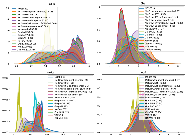
In this section, we provide additional experiments on QM9 (Ramakrishnan et al. 2014) and ZINC250k (Kusner, Paige, and Hernández-Lobato 2017) datasets (Table 4 and Table 5). To compute validity for MolGrow, we removed edges that exceed maximum atom valency. If a final graph contains more than one fragment, we keep only the biggest one. Validity without cleanup corresponds to a fraction of valid molecules when no additional manipulations are performed on the generated graph. We check validity using RDKit and additionally consider molecules with multiple components invalid. We provide property distribution plots for models trained on MOSES in Figure 5.
Appendix C Appendix C. Molecular property optimization
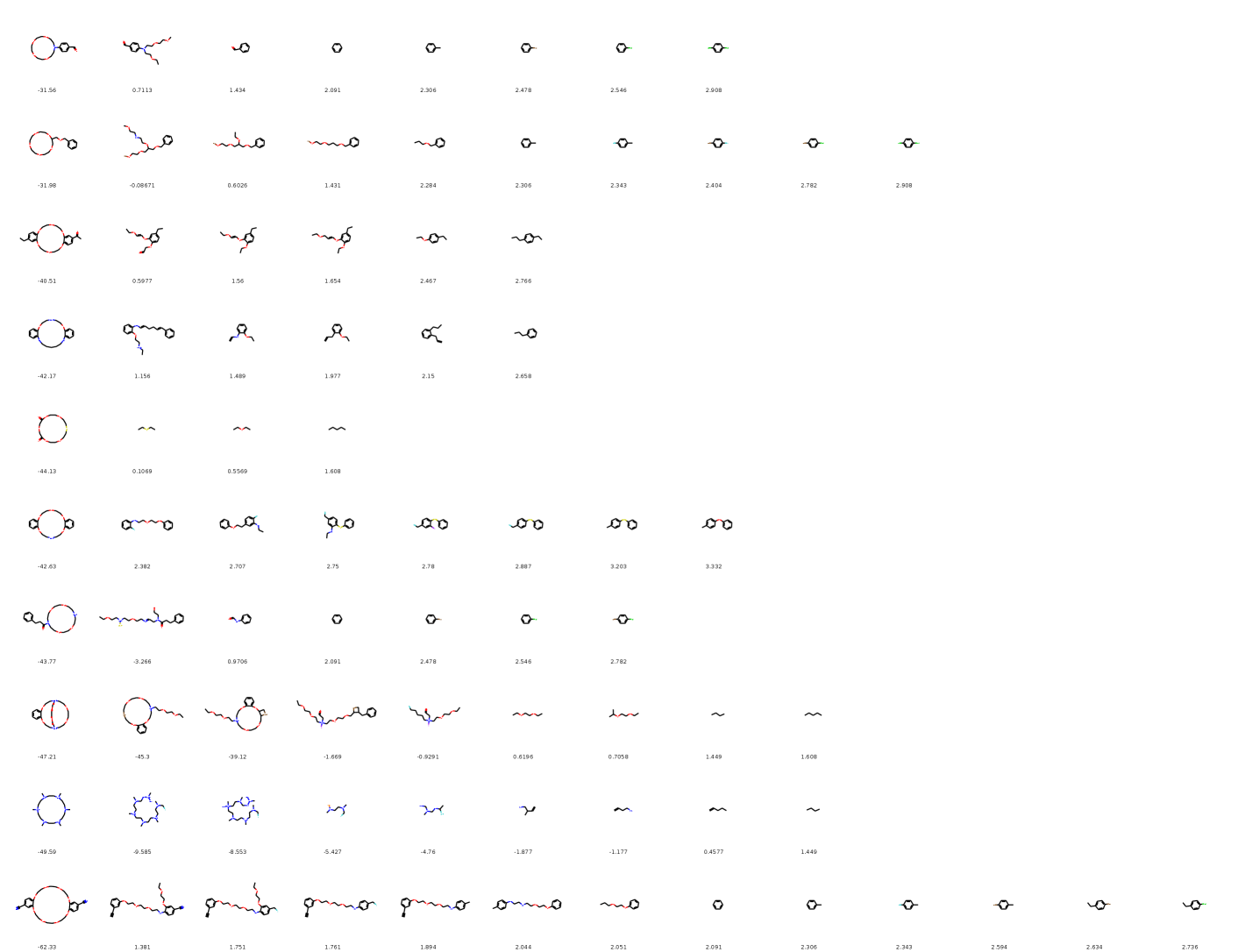
In this section, we illustrate genetic optimization of molecular properties. In Figures 11 and 13, we show best molecules in intermediate populations without consecutive duplicates. In Figures 12 and 14, we show the best molecules in the final population.
In Figure 6, Figure 7, and Figure 8 we provide random samples from MolGrow trained on QM9, ZINC and MOSES datasets correspondingly.
| Method | Validity | Validity without cleanup | Unique@10k | Novelty | Reconstruction |
|---|---|---|---|---|---|
| JT-VAE | 100% | - | 100% | 100% | 76.7% |
| MolecularRNN | 100% | 65% | 99.89% | 100% | - |
| GraphNVP | 42.6% | - | 94.8% | 100% | 100% |
| GraphAF | 100% | 68% | 99.1% | 100% | 100% |
| MoFlow | % | % | % | % | % |
| MolGrow | % | % | % | % | % |
| Method | Validity | Validity without cleanup | Unique@10k | Novelty | Reconstruction |
|---|---|---|---|---|---|
| GraphVAE | - | 55% | 76% | 61% | 55% |
| GraphNVP | 83% | - | 99.2% | 58.2% | 100% |
| GraphAF | 100% | 67% | 94.5% | 88.8% | 100% |
| MoFlow | % | % | % | % | % |
| MolGrow | % | % | % | % | % |
| Model | Valid () | Unique@1k () | Unique@10k () | FCD () | SNN () | Frag () | Scaf () | IntDiv () | IntDiv2 () | Filters () | Novelty () | ||||
| Test | TestSF | Test | TestSF | Test | TestSF | Test | TestSF | ||||||||
| Graph-based models | |||||||||||||||
| MolecularRNN | 1.0 | 0.999 | 0.9861 | 23.1302 | 24.1749 | 0.279 | 0.2681 | 0.5657 | 0.5579 | 0.0457 | 0.0075 | 0.9062 | 0.8985 | 0.6143 | 0.9996 |
| GraphVAE | 1.0 | 0.207 | 0.0495 | 49.3917 | 50.7191 | 0.2082 | 0.189 | 0.2304 | 0.2148 | 0.0 | 0.0 | 0.8238 | 0.7769 | 0.963 | 1.0 |
| GraphNVP | 1.0 | 0.999 | 0.9974 | 29.9517 | 31.2123 | 0.3057 | 0.2836 | 0.6297 | 0.6144 | 0.0266 | 0.0139 | 0.8574 | 0.8448 | 0.6008 | 0.9999 |
| GraphAF | 1.0 | 0.989 | 0.9707 | 21.85 | 23.2515 | 0.3056 | 0.2891 | 0.6513 | 0.6346 | 0.1255 | 0.0137 | 0.9036 | 0.8927 | 0.4145 | 0.9999 |
| MoFlow | 1.0 | 1.0 | 1.0 | 28.05 | 29.30 | 0.2554 | 0.2426 | 0.6858 | 0.6683 | 0.0224 | 0.0068 | 0.8923 | 0.8849 | 0.4126 | 0.9999 |
| Proposed model | |||||||||||||||
| MolGrow(fragment-oriented) | 1.0 | 1.0 | 0.998 | 5.7888 | 6.3861 | 0.4335 | 0.4208 | 0.9518 | 0.9464 | 0.6697 | 0.0769 | 0.8663 | 0.8599 | 0.8274 | 0.9938 |
| MolGrow(BFS) | 1.0 | 1.0 | 0.9999 | 9.2024 | 9.8472 | 0.3997 | 0.3891 | 0.9476 | 0.9414 | 0.6628 | 0.0631 | 0.8724 | 0.8665 | 0.6673 | 0.9928 |
| MolGrow(BFS on fragments) | 1.0 | 1.0 | 1.0 | 15.0707 | 15.9881 | 0.3379 | 0.3269 | 0.8902 | 0.8794 | 0.1875 | 0.0308 | 0.8883 | 0.8819 | 0.6169 | 0.9993 |
| MolGrow(random perm) | 1.0 | 0.967 | 0.8861 | 36.6702 | 37.9284 | 0.2292 | 0.2136 | 0.0729 | 0.0696 | 0.0002 | 0.0 | 0.8735 | 0.8616 | 0.5777 | 1.0 |
| MolGrow(GAT instead of CAGE) | 1.0 | 1.0 | 0.9953 | 6.4564 | 6.9704 | 0.4383 | 0.4263 | 0.9499 | 0.9449 | 0.6599 | 0.0827 | 0.8704 | 0.863 | 0.8367 | 0.9936 |
| MolGrow(No positional embeddings) | 1.0 | 1.0 | 0.9926 | 7.5529 | 8.1794 | 0.4242 | 0.4138 | 0.9320 | 0.9279 | 0.6029 | 0.0828 | 0.8744 | 0.8668 | 0.8177 | 0.9949 |
| SMILES and fragment-based models | |||||||||||||||
| CharRNN | 0.9884 | 1.0 | 0.9992 | 0.0615 | 0.4967 | 0.6109 | 0.5709 | 0.9999 | 0.9984 | 0.9269 | 0.107 | 0.8566 | 0.8507 | 0.996 | 0.8232 |
| VAE | 0.9766 | 1.0 | 0.9982 | 0.1094 | 0.5548 | 0.626 | 0.5776 | 0.9993 | 0.9987 | 0.9411 | 0.0485 | 0.8556 | 0.8496 | 0.9971 | 0.6871 |
| JTN-VAE | 1.0 | 1.0 | 0.9992 | 0.4224 | 0.9962 | 0.5561 | 0.5273 | 0.9962 | 0.9948 | 0.8925 | 0.1005 | 0.8512 | 0.8453 | 0.9778 | 0.9153 |