Multi-Agent Adversarial Training Using Diffusion Learning

In many machine learning algorithms, small malicious perturbations that are imperceptible to the human eye can cause classifiers to reach erroneous conclusions [1, 2, 3, 4, 5]. To mitigate the negative effect of adversarial examples, one methodology is adversarial training [6], in which clean training samples are augmented by adversarial samples by adding purposefully crafted perturbations. Due to the lack of an explicit definition for the imperceptibility of perturbations, additive attacks are usually restricted within a small bounded region. Most earlier studies, such as [7, 8, 6, 9, 10], have focused on studying adversarial training in the context of single agent learning. In this work, we devise a robust training algorithm for multi-agent networked systems by relying on diffusion learning [5, 11, 12], which has been shown to have a wider stability range and improved performance guarantees for adaptation in comparison to other decentralized strategies [5, 11, 12].

There of course exist other works in the literature that applied adversarial learning to a multiplicity of agents, albeit using a different architecture. For example, the works [13, 14, 15] employ multiple GPUs and a fusion center, while the works [16, 17, 18] consider graph neural networks. In this work, we focus on a fully decentralized architecture where each agent corresponds to a learning unit in its own right, and interactions occur locally over neighborhoods determined by a graph topology.

We formulate a sequential minimax optimization problem involving adversarial samples, and assume in this article that the perturbations are within an $\ell_{2}-$bounded region. We hasten to add though that the analysis can be extended to other norms, such as $\ell_{1}-$ and $\ell_{\infty}-$bounded perturbations. For simplicity, and due to space limitations, we consider the $\ell_{2}-$case here.

In the performance analysis, we examine the convergence of the proposed framework for convex settings due to space limitations, but note that similar bounds can be derived for nonconvex environments by showing convergence towards local minimizers. In particular, we show here that with strongly-convex loss functions, the proposed algorithm approaches the global minimizer within $O(\mu)$ after sufficient iterations, where $\mu$ is the step-size parameter.

One methodology for solving (1) is to first determine the inner maximizer in (2), thus reducing the minimax problem to a standard stochastic minimization formulation. Then, the traditional stochastic gradient method could be used to seek the minimizer. We denote the true maximizer of the perturbed loss function in (2) by

$\displaystyle\boldsymbol{\delta}_{k}^{\star}(w)\in\mathop{\mathrm{argmax}}\limits_{\left\|{\delta}_{k}\right\|\leq\epsilon}Q_{k}(w;\boldsymbol{x}_{k}+{\delta}_{k},\boldsymbol{y}_{k})$

(3)

where the dependence of $\boldsymbol{\delta}_{k}^{\star}$ on $w$ is shown explicitly. To apply the stochastic gradient method, we would need to evaluate the gradient of $Q(w;\boldsymbol{x}_{k}+\boldsymbol{\delta}_{k}^{\star}(w),\boldsymbol{y}_{k})$ relative to $w$, which can be challenging since $\boldsymbol{\delta}_{k}^{\star}(w)$ is also dependent on $w$. This difficulty can be resolved by appealing to Danskin’s theorem [19, 20, 21]. Let

$\displaystyle g(w)\overset{\Delta}{=}\max_{\left\|{\delta}_{k}\right\|\leq\epsilon}Q_{k}(w;\boldsymbol{x}_{k}+{\delta}_{k},\boldsymbol{y}_{k})$

(4)

Then, the theorem asserts that $g(w)$ is convex over $w$ if $Q_{k}(w;\cdot,\cdot)$ is convex over $w$. Moreover, $g(w)$ need not be differentiable over $w$ even when $Q_{k}(w;\cdot,\cdot)$ is differentiable. However, and importantly for our purposes, we can determine a subgradient for $g(w)$ by using the actual gradient of the loss evaluated at the worst perturbation, namely, it holds that

$\displaystyle\nabla_{w}Q_{k}(w;\boldsymbol{x}_{k}+\boldsymbol{\delta}_{k}^{\star},\boldsymbol{y}_{k})\in\partial_{w}g(w)$

(5)

where $\partial_{w}$ refers to the subdifferential set of its argument. In (5), the gradient of $Q_{k}(\cdot)$ relative to $w$ at the maximizer $\boldsymbol{\delta}_{k}^{\star}$ is computed by treating $\boldsymbol{\delta}_{k}^{\star}$ as a stand-alone vector and ignoring its dependence on $w$. When $\boldsymbol{\delta}_{k}^{\star}$ in (3) happens to be unique, then the gradient on the left in (5) will be equal to the right side, so that in that case the function $g(w)$ is differentiable.

Motivated by these properties, and using (5), we can now propose an algorithm to enhance the robustness of multi-agent systems to adversarial perturbations. To do so, we rely on the adapt-then-combine (ATC) version of the diffusion strategy [11, 12] and write down the following adversarial extension to solve (1)–(2)

		$\displaystyle\boldsymbol{x}_{k,n}^{\star}=\boldsymbol{x}_{k,n}+\boldsymbol{\delta}^{\star}_{k,n}$		(6a)
		$\displaystyle\boldsymbol{\phi}_{k,n}=\boldsymbol{w}_{k,n-1}-\mu\nabla_{w}Q_{k}(\boldsymbol{w}_{k,n-1};\boldsymbol{x}_{k,n}^{\star},\boldsymbol{y}_{k,n})$		(6b)
		$\displaystyle\boldsymbol{w}_{k,n}=\sum\limits_{\ell\mathcal{\in N}_{k}}a_{\ell k}\boldsymbol{\phi}_{\ell,n}$		(6c)

where

$$\boldsymbol{\delta}^{\star}_{k,n}\in\mathop{\mathrm{argmax}}\limits_{\left\|{\delta}_{k}\right\|\leq\epsilon}Q_{k}(\boldsymbol{w}_{k,n-1};\boldsymbol{x}_{k,n}+{\delta}_{k},\boldsymbol{y}_{k,n})$$

(7)

In this implementation, expression (6a) computes the worst-case adversarial example at iteration $n$ using the perturbation from $(\ref{max_k})$, while (6b) is the intermediate adaptation step in which all agents simultaneously update their parameters with step-size $\mu$. Relation (6c) is the convex combination step where the intermediate states $\boldsymbol{\phi}_{\ell,n}$ from the neighbors of agent $k$ are combined together. The scalars $a_{\ell k}$ are non-negative and they add to one over $\ell\in{\cal N}_{k}$.

This section analyzes the convergence of the adversarial diffusion strategy (6a)–(6c) for the case of strongly convex loss functions. We list the following assumptions, which are commonly used in the literature of decentralized multi-agent learning and single-agent adversarial training [11, 22, 23, 24, 25].

We remark that it also follows from Danskin’s theorem [19, 20, 21] that, when $Q_{k}(w;\cdot,\cdot)$ is $\nu-$strongly convex over $w$, then the adversarial risk $J_{k}({w})$ defined by (2) will be strongly convex. As a result, the aggregate risk $J(w)$ in (1) will be strongly-convex as well.

Note that (11) is automatically satisfied when all agents use the same loss function and collect data independently from the same distribution.

To evaluate the performance of the proposed framework (6a)–(6c), it is critical to compute the inner maximizer $\boldsymbol{\delta}_{k,n}^{\star}$ defined by (7). Fortunately, for some convex problems, such as logistic regression, the maximization in (7) has a unique closed-form solution, which will be shown in the simulation section. Thus, we analyze the convergence properties of (6a)–(6c) when $\boldsymbol{\delta}_{k,n}^{\star}$ is unique. We first establish the following affine Lipschitz result for the risk function in (2); proofs are omitted due to space limitations.

Contrary to the traditional analysis of decentralized learning algorithms where the risk functions $J_{k}(w)$ are generally Lipschitz, it turns out from (12) that under adversarial perturbations, the risks in (2) are now affine Lipschitz. This requires adjustments to the convergence arguments. A similar situation arises, for example, when one studies the convergence of decentralized learning under non-smooth losses — see [5, 26, 27].

To proceed with the convergence analysis, we introduce the gradient noise process, which is defined by

$$\boldsymbol{s}_{k,n}(\boldsymbol{w}_{k,n-1})=\nabla_{w}Q_{k}(\boldsymbol{w}_{k,n-1};\boldsymbol{x}_{k,n}^{\star},\boldsymbol{y}_{k,n})-\nabla_{w}J_{k}(\boldsymbol{w}_{k,n-1})$$

(13)

This quantity measures the difference between the approximate gradient (represented by the gradient of the loss) and the true gradient (represented by the gradient of the risk). The following result establishes some useful properties for the gradient noise process, namely, it has zero mean and bounded second-order moment (conditioned on past history).

The main convergence result is stated next; the proof is again omitted due to space limitations.

The above theorem indicates that the proposed algorithm enables the network to approach an $O(\mu)$-neighborhood of the robust minimizer $w^{\star}$ after enough iterations, so that the worst-case performance over all possible perturbations in the small region bounded by $\epsilon$ can be effectively minimized.

In this section, we illustrate the performance of the proposed algorithm using a logistic regression application. Let $\boldsymbol{\gamma}$ be a binary variable that takes values from $\{-1,1\}$, and $\boldsymbol{h}\in\mathbbm{R}^{M}$ be a feature variable. The robust logistic regression problem by a network of agents employs the risk functions:

$\displaystyle J_{k}(w)=\mathds{E}\max\limits_{\|{\delta}\|\leq\epsilon}\left\{\ln{(1+e^{-\boldsymbol{\gamma}(\boldsymbol{h}+{\delta})^{\sf T}{w}}})\right\}$

(18)

The analytical solution for the inner maximizer (i.e., the worst-case perturbation) is given by

$\displaystyle\boldsymbol{\delta}^{\star}=-\epsilon\boldsymbol{\gamma}\frac{\boldsymbol{w}}{\|\boldsymbol{w}\|}$

(19)

which is consistent with the perturbation computed from the fast gradient method (FGM) [7].

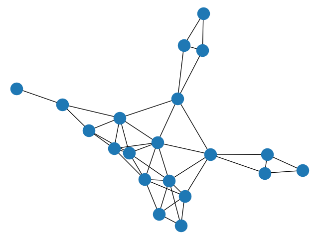
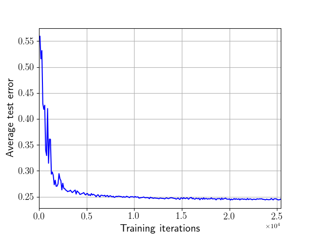
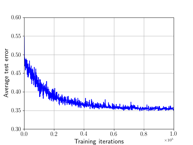
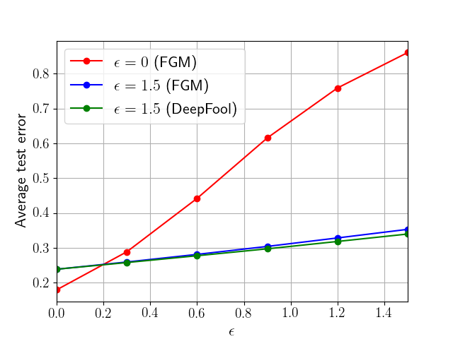
In our experiments, we use both the MNIST [28] and CIFAR10 [29] datasets, and randomly generate a graph with 20 nodes, shown in Fig. 1. We limit our simulations to binary classification in this example. For this reason, we consider samples with digits $0$ and $1$ from MNIST, and images for airplanes and automobiles from CIFAR10. We set the perturbation bound in (18) to $\epsilon=4$ for MNIST and $\epsilon=1.5$ for CIFAR10. In the test phase, we compute the average classification error across the network to measure the performance of the multi-agent system against perturbations of different strengths.

We first illustrate the convergence of our algorithm, as anticipated by Theorem 1. From Fig. 2, we observe a steady decrease in the classification error towards a limiting value.

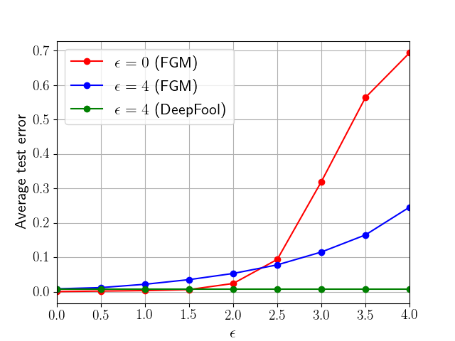
The robust behavior of the proposed algorithm is illustrated in Fig. 3 for both MNIST and CIFAR10. We explain the curves for MNIST and similar remarks hold for CIFAR10. In the simulation, we use perturbations generated in one of two ways: using the FGM worst-case construction and also using the DeepFool construction [5, 30]. The figure shows three curves. The red curve is obtained by training the network using the traditional diffusion learning strategy without accounting for robustness. The network is subsequently fed with worst-case perturbed samples (generated using FGM) during testing corresponding to different levels of $\epsilon$. The red curve shows that the classification error deteriorates rapidly. The blue curve repeats the same experiment except that the network is now trained with the adversarial diffusion strategy (6a)–(6c). It is seen in the blue curve that the testing error is more resilient and the degradation is better controlled. The same experiment is repeated using the same adversarially trained network, where the perturbed samples are now generated using DeepFool as opposed to FGM. Here again it is seen that the network is resilient and the degradation in performance is better controlled.

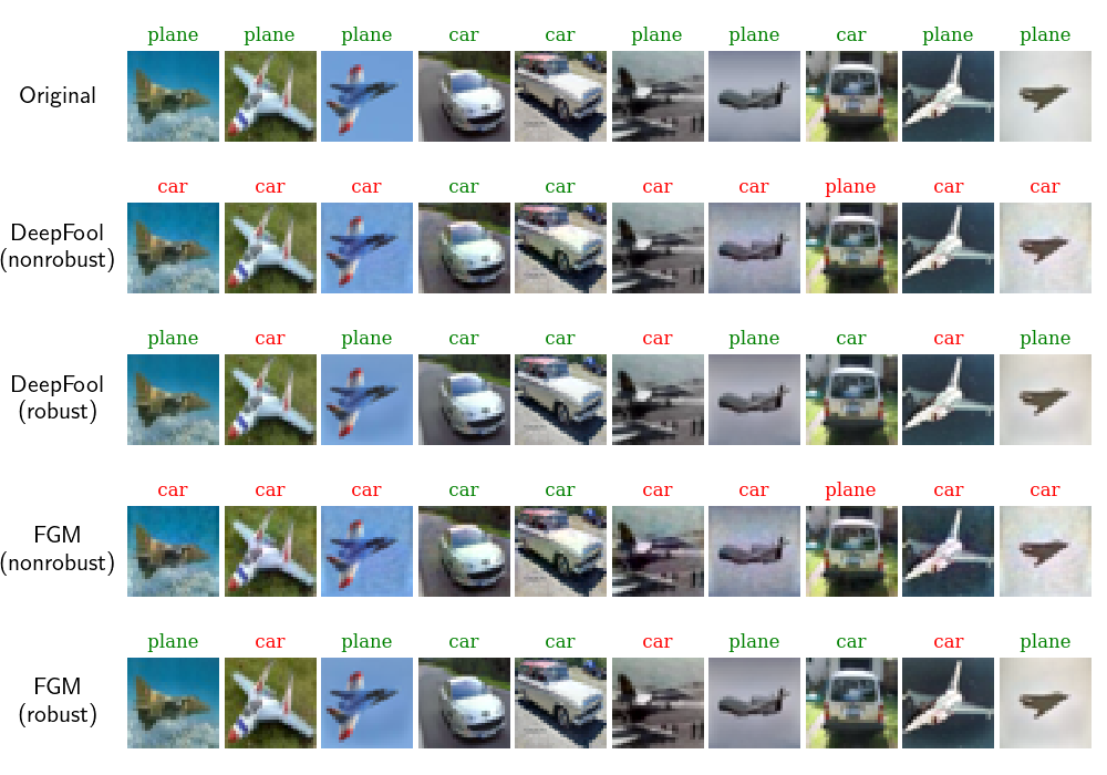
In Fig. 4, we plot some randomly selected CIFAR10 images, their perturbed versions, and the classification decisions generated by the nonrobust algorithm and its adversarial version (6a)–(6c). We observe from the figure that no matter which attack method is applied, the perturbations are always imperceptible to the human eye. Moreover, while the nonrobust algorithm fails to classify correctly in most cases, the adversarial algorithm is more robust and leads to fewer classification errors.

In this paper, we proposed a diffusion defense mechanism for adversarial attacks. We analyzed the convergence of the proposed method under convex losses and showed that it approaches a small $O(\mu)$ neighborhood around the robust solution. We further illustrated the behavior of the trained network to perturbations generated by FGM and DeepFool constructions and observed the enhanced robust behavior. Similar results are applicable to nonconvex losses and will be described in future work.

References

- [1] C. Szegedy, W. Zaremba, I. Sutskever, J. Bruna, D. Erhan, I. Goodfellow, and R. Fergus, “Intriguing properties of neural networks,” in Proc. International Conference on Learning Representations, Banff, 2014, pp. 1–10.
- [2] Y. Song, T. Kim, S. Nowozin, S. Ermon, and N. Kushman, “Pixeldefend: Leveraging generative models to understand and defend against adversarial examples,” in Proc. International Conference on Learning Representations, Vancouver, 2018, pp. 1–20.
- [3] R. Jia and P. Liang, “Adversarial examples for evaluating reading comprehension systems,” in Proc. Empirical Methods in Natural Language Processing, Copenhagen, 2017, pp. 1–11.
- [4] L. Pinto, J. Davidson, R. Sukthankar, and A. Gupta, “Robust adversarial reinforcement learning,” in Proc. International Conference on Machine Learning, Sydney, 2017, pp. 2817–2826.
- [5] A. H. Sayed, Inference and Learning from Data. Cambridge University Press, 2022.
- [6] A. Madry, A. Makelov, L. Schmidt, D. Tsipras, and A. Vladu, “Towards deep learning models resistant to adversarial attacks,” in Proc. International Conference on Learning Representations, Vancouver, 2018, pp. 1–23.
- [7] T. Miyato, A. M. Dai, and I. Goodfellow, “Adversarial training methods for semi-supervised text classification,” in Proc. International Conference on Learning Representations, Toulon, 2017, pp. 1–11.
- [8] I. Goodfellow, J. Shlens, and C. Szegedy, “Explaining and harnessing adversarial examples,” in Proc. International Conference on Learning Representations, San Diego, 2015, pp. 1–11.
- [9] P. Maini, E. Wong, and Z. Kolter, “Adversarial robustness against the union of multiple perturbation models,” in Proc. International Conference on Machine Learning, 2020, pp. 6640–6650.
- [10] H. Zhang, Y. Yu, J. Jiao, E. Xing, L. El Ghaoui, and M. Jordan, “Theoretically principled trade-off between robustness and accuracy,” in Proc. International Conference on Machine Learning, California, 2019, pp. 7472–7482.
- [11] A. H. Sayed, “Adaptation, learning, and optimization over networks,” Foundations and Trends in Machine Learning, vol. 7, pp. 311–801, 2014.
- [12] A. H. Sayed, “Adaptive networks,” Proc. IEEE, vol. 102, no. 4, pp. 460–497, 2014.
- [13] C. Qin, J. Martens, S. Gowal, D. Krishnan, K. Dvijotham, A. Fawzi, S. De, R. Stanforth, and P. Kohli, “Adversarial robustness through local linearization,” in Proc. Advances in Neural Information Processing Systems, Vancouver, 2019, pp. 13 824–13 833.
- [14] G. Zhang, S. Lu, S. Liu, X. Chen, P.-Y. Chen, L. Martie, L. Horesh, and M. Hong, “Distributed adversarial training to robustify deep neural networks at scale,” in Proc. Conference on Uncertainty in Artificial Intelligence, Eindhoven, 2022, pp. 2353–2363.
- [15] Y. Liu, X. Chen, M. Cheng, C.-J. Hsieh, and Y. You, “Concurrent adversarial learning for large-batch training,” in Proc. International Conference on Learning Representations, 2022, pp. 1–17.
- [16] F. Feng, X. He, J. Tang, and T.-S. Chua, “Graph adversarial training: Dynamically regularizing based on graph structure,” IEEE Transactions on Knowledge and Data Engineering, vol. 33, no. 6, pp. 2493–2504, 2021.
- [17] K. Xu, H. Chen, S. Liu, P. Y. Chen, T. W. Weng, M. Hong, and X. Lin, “Topology attack and defense for graph neural networks: An optimization perspective,” in Proc. International Joint Conference on Artificial Intelligence, Macao, 2019, pp. 3961–3967.
- [18] X. Wang, X. Liu, and C.-J. Hsieh, “Graphdefense: Towards robust graph convolutional networks,” arXiv preprint arXiv:1911.04429, pp. 1–9, 2019.
- [19] T. Lin, C. Jin, and M. Jordan, “On gradient descent ascent for nonconvex-concave minimax problems,” in Proc. International Conference on Machine Learning, 2020, pp. 6083–6093.
- [20] R. T. Rockafellar, Convex Analysis. Princeton University Press, 2015.
- [21] K. K. Thekumparampil, P. Jain, P. Netrapalli, and S. Oh, “Efficient algorithms for smooth minimax optimization,” in Proc. Advances in Neural Information Processing Systems, Vancouver, 2019, pp. 12 659–12 670.
- [22] A. Sinha, H. Namkoong, R. Volpi, and J. Duchi, “Certifying some distributional robustness with principled adversarial training,” in Proc. International Conference on Learning Representations, Vancouver, 2018, pp. 1–34.
- [23] S. Vlaski and A. H. Sayed, “Diffusion learning in non-convex environments,” in Proc. IEEE ICASSP, Brighton, 2019, pp. 5262–5266.
- [24] S. Vlaski and A. H. Sayed, “Distributed learning in non-convex environments—part i: Agreement at a linear rate,” IEEE Transactions on Signal Processing, vol. 69, pp. 1242–1256, 2021.
- [25] S. Vlaski and A. H. Sayed, “Distributed learning in non-convex environments—part ii: Polynomial escape from saddle-points,” IEEE Transactions on Signal Processing, vol. 69, pp. 1257–1270, 2021.
- [26] B. Ying and A. H. Sayed, “Performance limits of stochastic sub-gradient learning, Part I: Single agent case,” Signal Processing, vol. 144, pp. 271–282, 2018.
- [27] B. Ying and A. H. Sayed, “Performance limits of stochastic sub-gradient learning, Part II: Multi-agent case,” Signal Processing, vol. 144, pp. 253–264, 2018.
- [28] L. Deng, “The mnist database of handwritten digit images for machine learning research,” IEEE Signal Processing Magazine, vol. 29, no. 6, pp. 141–142, 2012.
- [29] A. Krizhevsky, V. Nair, and G. Hinton, “Cifar-10 (canadian institute for advanced research).” [Online]. Available: http://www.cs.toronto.edu/ kriz/cifar.html
- [30] S.-M. Moosavi-Dezfooli, A. Fawzi, and P. Frossard, “DeepFool: a simple and accurate method to fool deep neural networks,” in Proc. IEEE CVPR, Las Vegas, 2016, pp. 2574–2582.