Multi-charged moments of two intervals in conformal field theory
Abstract
We study the multi-charged moments for two disjoint intervals in the ground state of two dimensional CFTs with central charge and global symmetry: the massless Dirac field theory and the compact boson (Luttinger liquid). For this purpose, we compute the partition function on the higher genus Riemann surface arising from the replica method in the presence of background magnetic fluxes between the sheets of the surface. We consider the general situation in which the fluxes generate different twisted boundary conditions at each branch point. The obtained multi-charged moments allow us to derive the symmetry resolution of the Rényi entanglement entropies and the mutual information for non complementary bipartitions. We check our findings against exact numerical results for the tight-binding model, which is a lattice realisation of the massless Dirac theory.
1 Introduction
As Schrödinger already recognised one century ago, entanglement is at the core of quantum mechanics. Nowadays it turns out to be the fundamental notion behind many quantum phenomena, from quantum algorithms nc-10 to gravity Rangamani ; nrt-09 , passing by critical phenomena and topological phases of matter intro1 ; intro2 ; eisert-2010 ; intro3 , triggering unexpected connections between apparently far branches of physics. At the center of all these ideas, we find the (Rényi) entanglement entropies which are powerful entanglement measures that provide fundamental insights about the investigated system or theory. They are defined as follows. Let us consider an extended quantum system in a pure state and a spatial bipartition into and . The subsystem is described by the reduced density matrix and the associated Rényi entropies are given by the moments of as
| (1) |
where we assume that is an integer number. After the analytic continuation to complex values of , the limit of Eq. (1) yields the von Neumann entanglement entropy
| (2) |
For bipartite systems in a pure state, the von Neumann and Rényi entropies can be used as measures of the entanglement shared between the two complementary parts. One of the most interesting properties of entanglement entropies is that they are sensitive to criticality. In particular, for one-dimensional gapless systems, if is a single interval, then the ground state entanglement entropy breaks the area law and is proportional to the central charge of the 1+1 dimensional CFT that describes the low-energy spectrum of the system cw-94 ; hlw-94 ; cc-04 ; cc-09 .
In the case considered in this work in which consists of two subsystems and , i.e. , the ground-state entanglement entropy depends on the full operator content of the CFT, encoding all the conformal data of the model Caraglio ; Furukawa ; twist2 ; cct-11 . It is important to remark that, in this situation, the entanglement entropies quantify the entanglement between and but not between the two parts of , for which one must resort to other entanglement measures such as negativity neg-qft ; neg-qft-2 ; ctt-13 ; Alba13 ; Coser3 ; Ares ; Rockwood . Nevertheless, from the entanglement entropies, it is possible to construct the following quantity, dubbed mutual information,
| (3) |
which is a measure of the total correlations between and . The computation of two-interval Rényi entanglement entropies is a difficult problem, even for minimal CFTs Dupic ; Ares , as it boils down in general to determine the partition function of the theory on a higher genus -sheeted Riemann surface twist2 ; cct-11 . In fact, exact analytic expressions are only available for the free theories or special limits Furukawa ; twist2 ; cct-11 ; CFH ; Alba ; Alba2 ; twist3 ; CoserTagliacozzo ; DeNobili ; Coser2 ; rtc-18 ; HLM13 ; gkt-21 ; Casini ; g-21 ; b-19 ; bds-20 . Moreover, the analytic continuation in to obtain Eq. (2) is still a challenging open issue.
In recent times, a question that has attracted much attention is how entanglement decomposes into the different symmetry sectors in the presence of global conserved charges lr-14 ; goldstein ; xavier . Various reasons have motivated the interest in this problem. The effect of symmetries on entanglement can be investigated experimentally fis ; Azses ; Neven ; Vitale and, moreover, understanding how entanglement arises from the symmetry sectors is crucial to better grasp some quantum features, for example in non-equilibrium dynamics fis . Also at more practical level, it can help to speed-up the numerical algorithms to simulate quantum many-body systems xavier . All that has been the breeding ground for a plethora of works that analyse the resolution of entanglement from different perspectives: spin chains lr-14 ; Vitale ; Neven ; riccarda ; SREE2dG ; goldstein2 ; MDC-19-CTM ; ccgm-20 ; wv-03 ; bhd-18 ; bcd-19 ; byd-20 ; mrc-20 ; tr-19 ; ms-21 ; amc-22 ; jones-22 ; pvcc-22 , integrable quantum field theories MDC-20 ; hcc-21 ; hcc-a-21 ; hc-20 ; chcc-a22 , CFTs goldstein ; xavier ; goldstein1 ; crc-20 ; MBC-21 ; Chen-21 ; Capizzi-Cal-21 ; Hung-Wong-21 ; cdm-21 ; boncal-21 ; eim-d-21 ; Chen-22 ; Ghasemi-22 ; mt-22 ; ms-21 , holography znm-20 ; wznm-21 ; znwm-22 ; bbcg-22 , out-of-equilibrium pbc-21-1 ; pbc-21 ; fg-21 ; pbc-22 ; sh-22 ; chen-22-2 and disordered systems trac-20 ; kusf-20 ; kusf-20b ; kufs-21-1 or topological matter clss-19 ; ms-20 ; Azses-Sela-20 ; ahn-20 ; ads-21 ; ore-21 to mention some of them. In order to analyse entanglement in each symmetry sector, quantities such as the symmetry-resolved entanglement entropy lr-14 ; goldstein ; xavier and the symmetry-resolved mutual information pbc-21 have been proposed. As shown in Ref. goldstein , symmetry-resolved entropies are intimately related to the charged moments of the reduced density matrix , which were independently studied in holographic theories Belin-Myers-13-HolChargedEnt ; cms-13 ; cnn-16 ; d-16 ; d-17 ; ssr-17 ; shapourian-19 . Similarly to the moments of , they can be interpreted as the partition function of the field theory on a Riemann surface, which is now coupled to an external magnetic flux. Partition functions with a background gauge field have been also introduced as non-local order parameters to detect symmetry-protected topological phases in interacting fermionic systems ssr1-17 ; ssr-16 .
The symmetry resolution of entanglement in the two-interval case has not been much explored in CFT. Ref. wznm-21 studies it at large central charge, in the context of holography, while, in Ref. Chen-22 , the charged Rényi negativity is analysed for the complex free boson. Here we take a different charge for each part of , which leads to introduce the multi-charged moments of . This non-trivial generalisation of the charged moments, first considered in Ref. pbc-21 in the context of quench dynamics, is the main subject of this work. In CFT, they correspond to the partition function on the -sheeted Riemann surface, but with the insertion of a different magnetic flux across each subset (interval) of . We compute the multi-charged moments analytically for the ground state of two bidimensional CFTs with central charge and global symmetry— the massless Dirac field theory and the free compact boson— generalising the expressions for the (neutral) Rényi entropies found in Refs. CFH and twist2 respectively. From the multi-charged moments, we derive the ground state symmetry-resolved entanglement entropy and mutual information of two disjoint intervals.
The paper is organised as follows: in Sec. 2, we define the symmetry-resolved entanglement and mutual information as well as the multi-charged moments, and we briefly describe the general approach to compute the latter in CFTs. We then move on to calculate the multi-charged moments for the ground state of the massless Dirac field theory in Sec. 3 and of the free compact boson in Sec. 4. In Sec. 5, we apply the previous results to obtain the symmetry-resolution of the mutual information in these theories. When possible, we benchmark the analytic expressions with exact numerical calculations for lattice models in the same universality class. We draw our conclusions in Sec. 6 and we include three appendices, with more details about the analytical and numerical computations.
2 Definitions
In this section, we first give the definition of the symmetry-resolved entanglement entropy and mutual information for a subsystem composed of two disjoint regions. We explain their relation with the multi-charged moments of the reduced density matrix, and we introduce the replica method to calculate them in CFTs.
2.1 Symmetry-resolved entanglement entropies and mutual information
As we already pointed out in Sec. 1, we take a spatial bipartition of an extended quantum system in a pure state , with made of two disconnected regions, . We assume that the system is endowed with a global symmetry generated by a local charge . Given the partition of the system in different subsets, we can consider the charge operator in each of them; for example, in region , it can be obtained as . If is an eigenstate of , the density matrix commutes with , i.e. , and, by taking the trace over , we find that . This implies that the reduced density matrix presents a block diagonal structure, in which each block corresponds to an eigenvalue of . That is,
| (4) |
where is the projector onto the eigenspace associated to the eigenvalue and is the probability of obtaining as the outcome of a measurement of . Notice that Eq. (4) guarantees the normalisation for any .
The amount of entanglement between and in each symmetry sector can be quantified by the symmetry-resolved Rényi entropies, defined as
| (5) |
Taking the limit in this expression, we obtain the symmetry-resolved entanglement entropy,
| (6) |
According to the decomposition of Eq. (4), the total entanglement entropy in Eq. (2) can be written as nc-10
| (7) |
where is known as configurational entropy and quantifies the average contribution to the total entanglement of all the charge sectors fis ; wv-03 ; bhd-18 ; bcd-19 , while is called number entropy and takes into account the entanglement due to the fluctuations of the value of the charge within the subsystem fis ; kusf-20 ; kusf-20b ; ms-20 ; kufs-21 ; zshgs-20 ; kufs-21b .
Since the total charge in is the sum of the charge in and , , then the reduced density matrices , of and can be independently decomposed in charged sectors as we did for in Eq. (4). Therefore, we can define the symmetry-resolved entropies , for the regions and analogous to Eq. (5) for , with . In Ref. pbc-21 , it has been proposed to define the symmetry-resolved mutual information as
| (8) |
The quantity , normalised as
| (9) |
is the probability that a simultaneous measurement of the charges and yields and , respectively, while the charge of the whole system is fixed to . Although Eq. (8) is a natural definition, is not in general a good measure of the total correlations between and within each charge sector since, in some cases, it can be negative pbc-21 . Nevertheless, we find interesting to investigate this quantity given that it provides a decomposition for the total mutual information (8) similar to the one reported in Eq. (7) for the entanglement entropy,
| (10) |
where is the number mutual information.
2.2 Charged moments and symmetry resolution
The computation of the symmetry-resolved entanglement entropies and mutual information from the definitions (5) and (8) requires the knowledge of the entanglement spectra of , and and their symmetry resolution. However, this is usually a very difficult task, in particular if one is interested in analytical expressions. Alternatively, one can employ the charged moments of the reduced density matrices. For , they are defined as
| (11) |
Similar quantities can also be introduced for the two subsystems and that constitute by replacing and by and , . If we take now their Fourier transform,
| (12) |
the symmetry-resolved entanglement entropies of the subsystem are given by goldstein ; xavier
| (13) |
In a similar manner, replacing with and , we can obtain the symmetry-resolved entanglement entropies of the two components of .
Notice that, for computing the symmetry-resolved mutual information of Eq. (8), we need to determine , i.e. the probability that a measurement of and gives and respectively, with fixed to . In order to calculate it, we consider the generalisation of the charged moments in Eq. (11) introduced for the first time in Ref. pbc-21 ,
| (14) |
We refer to them as multi-charged moments. When , Eq. (14) reduces to the charged moments of of Eq. (11). If we take the Fourier transform of Eq. (14),
| (15) |
then can be interpreted as the probability of having and as outcomes of a measurement of and respectively, independently of the value of . Therefore, it satisfies the normalisation
| (16) |
and can be calculated as the conditional probability
| (17) |
which fulfills Eq. (9).
2.3 Charged moments in CFT
In the rest of the paper, we will analyse the previous quantities in -dimensional CFTs with a global symmetry. We will assume that the entire system is in the ground state and that the spatial dimension is an infinite line which we will divide into two parts and , with made up of two disjoint intervals, namely . If we denote by and the lengths of the two intervals and their separation, we have
| (18) |
where we have also introduced the cross ratio of the four end-points, which takes values between and .
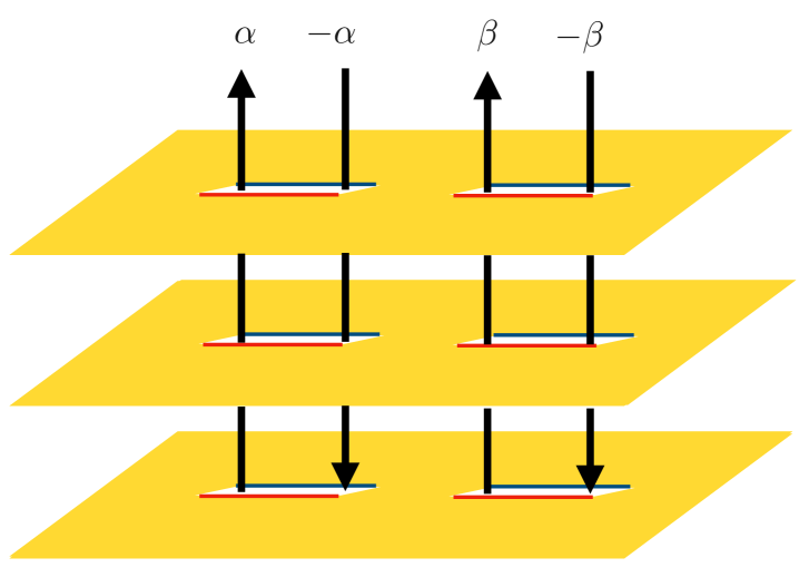
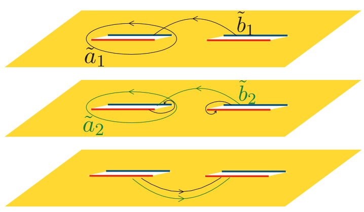
As explained in detail in Refs. cc-04 ; cc-09 , using the path integral representation of , the moments are equal to the partition function of the CFT on a Riemann surface, which we call , obtained as follows. We take the complex plane where the CFT is originally defined and we perform two cuts along the intervals and . Then we replicate times the cut plane and we glue the copies together along the cuts in a cyclical way as we illustrate in Fig. 1. We eventually obtain an -sheeted Riemann surface of genus , which is symmetric under the cyclic permutation of the sheets.
Alternatively, instead of replicating the space-time where the CFT is initially defined, one can take copies of the CFT on the complex plane and quotient it by the symmetry under the cyclic exchange of the copies. We then get the orbifold theory . The moments are equal to the four-point correlation function on the complex plane cc-04 ; ccd-08 ,
| (19) |
where and are dubbed as twist and anti-twist fields k-87 ; dixon ; cc-04 ; ccd-08 . They implement in the orbifold the multivaluedness of the correlation functions on the surface when we go around its branch points. In fact, the winding around the point where () is inserted maps a field living in the copy of the orbifold into the copy (), that is
| (20) |
The twist and anti-twist fields are spinless primaries with conformal weight
| (21) |
where is the central charge of the initial CFT.
The charged moments of can also be computed employing the previous frameworks. As argued in Ref. goldstein , the operator can be interpreted as a magnetic flux between the sheets of the surface , such that a charged particle moving along a closed path that crosses all the sheets acquires a phase . For the multi-charged moments introduced in Eq. (14), we have to insert two different magnetic fluxes and at the cuts and respectively, as we pictorially show in Fig. 1. They can be implemented by a local operator that generates a phase shift along the real interval . Then the charged moments are equal to the four-point correlation function on the surface
| (22) |
In the orbifold theory, the magnetic flux can be incorporated by considering the composite twist field . Thus, if we take a field in the copy of the orbifold, then the winding around the point where is inserted gives rise to a phase ,
| (23) |
The same applies to the composite anti-twist field , which takes a field from the copy to adding a phase . Therefore, Eq. (22) can be re-expressed as the four-point function on the complex plane
| (24) |
In Ref. goldstein , it is shown that, if is a spinless primary operator with conformal weight , then so are the composite twist and anti-twist fields, with conformal weights
| (25) |
One can further consider other configurations for the magnetic fluxes between the sheets of the Riemann surface . In general, if we assume that a particle gets a different phase when it goes around each branch point, provided they satisfy the neutrality condition , then the partition function of this theory is given by
| (26) |
or, in terms of the composite twist fields, by
| (27) |
Then the multi-charged moments can be treated as the particular case in which and, due to the neutrality condition, .
In Sec. 3, we will compute the charged moments —and more in general the partition functions —for the massless Dirac fermion using the orbifold theory . On the other hand, in Sec. 4, we will adopt a geometric approach to obtain the multi-charged moments of the compact boson from the correlation function on the Riemann surface of Eq. (26).
3 Free massless Dirac field theory
The massless Dirac field theory is described by the action
| (28) |
where . The matrices can be represented in terms of the Pauli matrices as and . The action of Eq. (28) exhibits a global symmetry: it is invariant if the fields are multiplied by a phase, i.e. and . By Noether’s theorem, this symmetry is related to the conservation of the charge .
The ground state entanglement of a subsystem made up of multiple disjoint intervals in the ground state of this theory was first investigated in Ref. CFH . For the case of two disjoint intervals, , it was found that the moments of are
| (29) |
where is a non-universal constant.
In this section, we will compute the multi-charged moments of Eq. (14) in the ground state of the massless Dirac field theory. We will extend the approach introduced in Ref. CFH for the moments of Eq. (29). Similar techniques have been exploited in Ref. MDC-20 for studying the charged moments of Eq. (11), when is a single interval, in two dimensional free massless Dirac theories and in Ref. MBC-21 in the context of the charge imbalance resolved negativity. We will benchmark our analytical results with exact numerical calculations in a lattice model.
3.1 Charged moments
In Sec. 2, we explained that the partition function can be obtained either by considering the theory on a complicated Riemann surface or by replicating it -times and working with the orbifold on the complex plane. For the massless Dirac field theory, the latter approach is more convenient. Thus, let us take the -component field
| (30) |
where is the Dirac field on the -th copy of the system. Eq. (23) describes the effect of the composite twist fields on the components of when going around the end-points of the subsystem . This transformation can be encoded in the matrix
| (31) |
In the general case of Eq. (27), transforms according to when winding around the point and to the transpose matrix when going around the point , with . The matrix in Eq. (31), sometimes called twist matrix, was introduced for the case in Refs. CFH ; ccd-08 and for general in Ref. MDC-20 . Its eigenvalues are of the form
| (32) |
By simultaneously diagonalising all the with a unitary transformation (which is independent of ), we can recast the replicated theory in decoupled fields on the plane, which are multi-valued,
| (33) |
Notice that this technique, known as diagonalisation in the replica space, can be applied only to free theories since, otherwise, the -modes do not decouple. For the free massless Dirac theory, this allows us to write the Lagrangian of the replicated theory as
| (34) |
Following this approach, the partition function of Eq. (27) factorises into
| (35) |
where is the partition function for a Dirac field with the boundary conditions of Eq. (3.1).
The main difference between the partition functions and the standard computation of Ref. CFH for Rényi entropies is that the boundary conditions of the multi-valued fields around the branch points now depend on the phases . This multivaluedness can be removed, as done in CFH for , by introducing an external gauge field coupled to single-valued fields . In fact, if we apply the singular gauge transformation
| (36) |
then the Lagrangian for the -th mode can be rewritten as
| (37) |
with the advantage of absorbing the phase around the end-points of into the gauge field. The only requirement that in Eq. (36) must satisfy is that, integrated along any closed curve that encircles the end-points of , the boundary conditions of Eq. (3.1) for must be reproduced. For this purpose, we require
| (38) |
where and are closed contours around the end-points of the -th interval. Moreover, we have to impose that, if does not enclose any end-point, then . Applying the Stoke’s theorem, the conditions of Eqs. (38) can be expressed in differential form,
| (39) |
Once the transformation of Eq. (36) is performed, the partition function of the -th mode is equal to the vacuum expectation value
| (40) |
where is the conserved Dirac current for each mode. Eq. (40) can be easily computed via bosonisation CFH , which allows us to write the current in terms of the dual scalar field such that . If we use this result in Eq. (40), and we apply Eq. (39), then is equal to the following correlation function of vertex operators
| (41) |
Notice that the neutrality condition ensures that the latter correlator does not vanish. The correlation function of vertex operators in the complex plane is well-known (see, for instance, Ref. difrancesco ) and, therefore, Eq. (41) can be easily calculated. Plugging the result into Eq. (35) and performing the product over , we obtain
| (42) |
where is the cross-ratio defined in Eq. (18). When we take and in this expression, we get the multi-charged moments in Eq. (14) as
| (43) |
We assume that all the length scales in this formula have been regularised through a UV cutoff which is included in the multiplicative constant .
An interesting case to analyse is when the two intervals and become adjacent; that is, when . In that limit, the cross-ratio tends to one such that
| (44) |
and Eq. (43) vanishes. Nevertheless, in this regime, the distance must be regarded as another UV cutoff, which can be absorbed in the multiplicative constant . Therefore, from Eqs. (44) and (43), one expects
| (45) |
which agrees with the fact that, according to Eq. (24), the multi-charged moments must tend to the three-point function of primaries , in the limit .
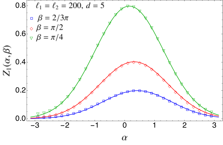
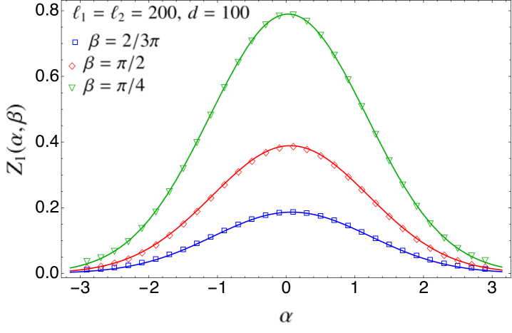
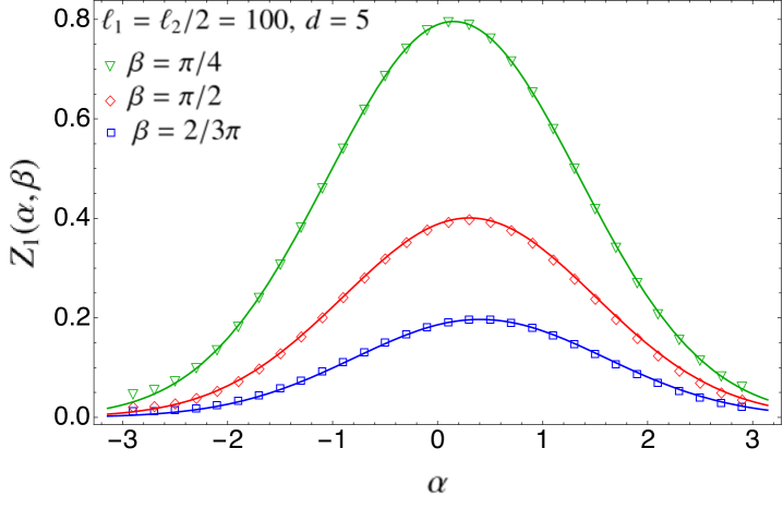
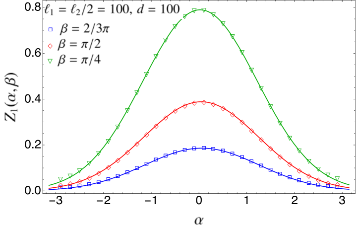
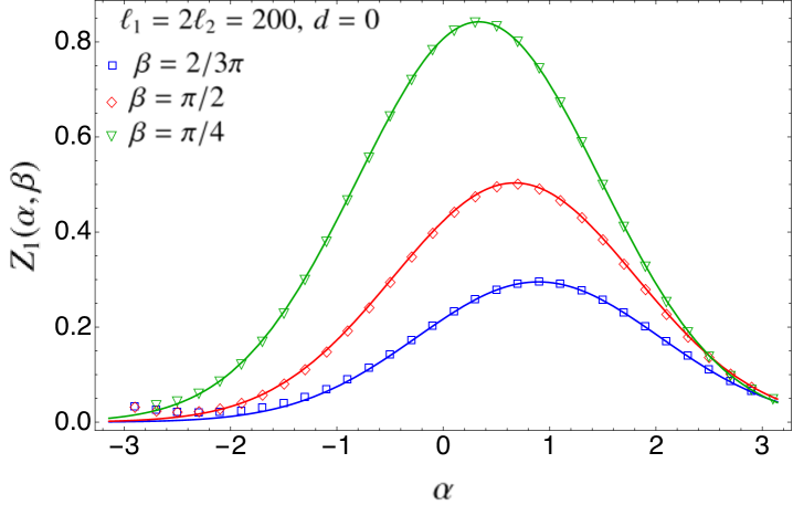
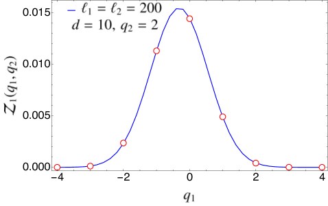
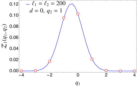
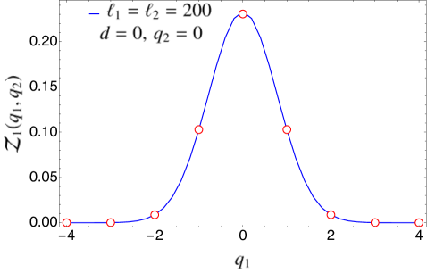
In Fig. 2, we check the expressions obtained in Eqs. (43) and (45) for with exact numerical calculations performed in the tight-binding model, which is a chain of non-relativistic free fermions whose scaling limit is described by the massless Dirac field theory. The details of the numerical techniques employed are given in Appendix A. In order to compare Eqs. (43) and (45) with the numerical data, we need the concrete expression of the non-universal factors and for this particular model. When the two intervals and are far away, that is in the limit , the multi-charged moments of factorise into those of and ,
| (46) |
Therefore, one expects to be the product of the two non-universal constants associated to and as single intervals. The latter were obtained for the tight-binding model in Ref. riccarda by exploiting the asymptotic properties of Toeplitz determinants. We can also apply here those results, taking into account that each interval is associated to a different flux, either or . Then we have
| (47) |
where riccarda
| (48) |
Expanding up to quadratic order in , then Eq. (47) can be approximated as
| (49) |
where and
| (50) |
In the limit of adjacent intervals, given by Eq. (45), the multiplicative constant cannot be determined using the known results for Toeplitz determinants. However, we can conjecture an analytical approximation for it at quadratic order in and . When , we can associate to each end-point of the intervals , and the fluxes , and respectively. From the results for one interval of Ref. riccarda , one can conjecture that each end-point with flux contributes with a factor to the constant , if we restrict to terms up to order . Therefore, the combination of all the fluxes in our case should contribute with a total factor . We then expect that should be well be approximated by
| (51) |
When , the expression above simplifies to the multiplicative constant for the moments of a single interval obtained in Ref. JK04 . In spite of the heuristic reasoning of this result, in Fig. 2, we check its validity by comparing it against exact numerical data.
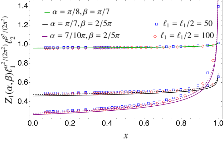
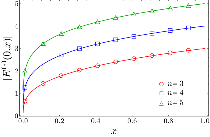
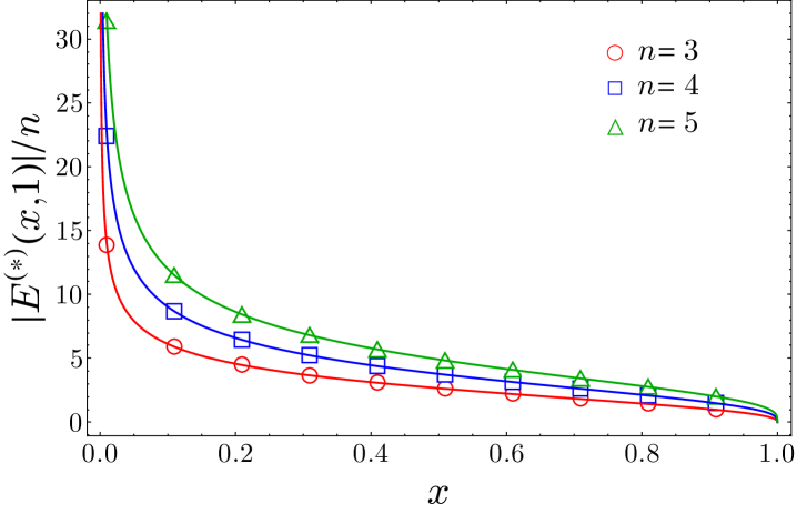
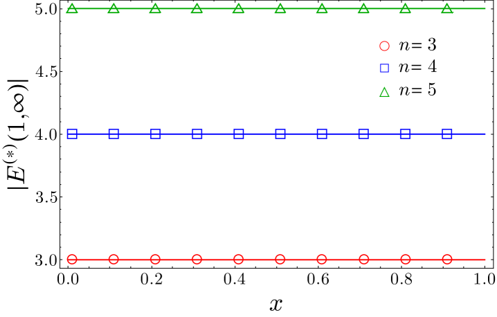
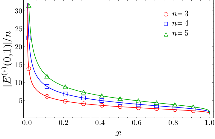
In the top and middle panels of Fig. 2, we study as function of , for various values of , , and . The points correspond to the exact numerical values obtained as we described in Appendix A, while the solid curves are the analytic prediction of Eq. (43), taking as multiplicative constant that in Eq. (47). We find an excellent agreement. In the bottom left panel, we analyse the case of adjacent intervals (). The numerical data for are in very good agreement with the analytical expression (solid curves) of Eq. (45), using Eq. (51) as multiplicative constant. Finally, in the bottom right panel, we plot as function of the cross-ratio , for various values of , , and . The curves represent the prediction of Eq. (43). The continuous ones correspond to take as non-universal constant the full expression of Eq. (47), while for the dashed ones we have used the quadratic approximation of Eq. (49). The agreement between the analytic prediction and the numerical data is extremely good, even considering the quadratic approximation for the non-universal constant. As expected, this agreement is better for small values of and , while, around , we need to take larger subsystem sizes , in order to suppress the finite-size corrections which are well-known and characterised for the charged moments with a single flux insertion riccarda .
4 Free compact boson
The second theory we focus on in this manuscript is the free compact boson, which is the CFT of the Luttinger liquid, and whose action reads
| (52) |
The target space of the real field is compactified on a circle of radius , i.e. with . The compactification radius is related to the Luttinger parameter as . The action of Eq. (52) is invariant under the transformation which, due to the compact nature of , realises a global symmetry. The associated conserved charge is .
The moments of the ground state reduced density matrix of this theory are well-known. An exact analytic expression for the two-interval case was obtained in Ref. twist2 , which was generalised to an arbitrary number of disjoint intervals in Ref. CoserTagliacozzo . In particular, for two intervals, it reads twist2
| (53) |
where is a non-universal constant and
| (54) |
We denote by the Riemann-Siegel Theta function
| (55) |
with characteristics , and a complex matrix. In Eq. (54), the characteristics are zero and, therefore, we have used the standard shorthand notation . The matrix in Eq. (54) has entries given by
| (56) |
and
| (57) |
with . The function is invariant under and it is normalised such that . Although the moments of are known for all the integer , its analytic continuation to complex and, consequently, the von Neumann entropy of Eq. (2) is still not available for all the values of the Luttinger parameter.
A remarkable contact point between the theories described by the actions of Eqs. (28) and (52) is the case . Notice that, when the Luttinger parameter takes this value, the function in Eq. (54) simplifies to =1 and the moments of Eq. (53) for the massless compact boson present the same universal dependence on , and as the ones in Eq. (29) for the massless Dirac fermion. A detailed discussion on this identity can be found in Ref. HLM13 , where it is explained the reason why, although these two theories are not related by a duality, their partition functions on the Riemann surfaces arising in the two-interval replica method are actually equal. Here we find that this identity extends to the partition functions on the surface with different twisted boundary conditions at each branch point. In general, when is made up of more than two intervals and the Rényi index is larger than two, the moments of the reduced density matrix in these CFTs (and the corresponding Rényi entropies) are different HLM13 .
4.1 Charged moments
We now generalise the result (53) to the multi-charged moments in Eq. (14). Starting from Eq. (22), we will compute them as the four-point function of the field on the Riemann surface . Since the conserved current is proportional to , is identified in this case with the vertex operator goldstein
| (58) |
which has conformal dimensions
| (59) |
In the following, it will be useful to introduce the rescaled Luttinger paratemeter in order to lighten the expressions.
Without loss of generality, let us consider that the end-points of subsystem are , , and . Using Eq. (27), and given that the composite twist fields are primaries, we can eventually obtain the expression for an arbitrary set of end-points through a global conformal transformation. Therefore, according to Eq. (22), the multi-charged moments can be derived from the four-point correlation function of the vertex operators of Eq (58)
| (60) |
on the -sheeted Riemann surface with branch points at , , and . This surface of genus can be described by the complex curve
| (61) |
The correlator of vertex operators on a general Riemann surface of arbitrary genus was obtained in Ref. Verlinde . In order to give the explicit expression in our case, we need to introduce some notions about Riemann surfaces Fay .
There are different parameterisations of the moduli space of genus Riemann surfaces. One possibility is through the matrix of periods, which we denote by . This is a symmetric matrix with positive definite imaginary part. Notice that, according to Eq. (61), the Riemann surface is parametrised by the cross-ratio . Therefore, the corresponding matrix of periods only depends on , i.e. . In order to define it, we need first to specify a particular homology basis for , i.e. a basis of oriented non-contractible curves on the surface, which we denote by and , with . The detailed description of the specific basis that we consider is given in Appendix B. We also have to choose a basis of holomorphic differentials , , normalised with respect to the cycles. That is,
| (62) |
Then the matrix of periods is defined as
| (63) |
For the surface , the normalised holomorphic differentials read
| (64) |
In Appendix B, we thoroughly explain the derivation of the expression for . Inserting it in Eq. (63), it is then easy to show that the entries of the matrix of periods are precisely those of Eq. (56).
If we now consider four vertex operators inserted at generic points in the surface and with arbitrary dimensions satisfying the neutrality condition , then its correlation function is of the form Verlinde
| (65) |
In this expression, we denote by the prime form of the surface , which we will define precisely later, and is the Abel-Jacobi map, which relates a point in the surface to a point in the genus complex torus , where . This map can be written in terms of the normalised holomorphic differentials of Eq. (64) as
| (66) |
where we have taken as origin the branch point . The images under the Abel-Jacobi map of the points , , , and , where the vertex operators in Eq. (60) are inserted, can be easily computed using Eq. (64) and applying the identities of Eq. (127). Then we find
| (67) | |||||
| (68) | |||||
| (69) | |||||
| (70) |
where and with
| (71) |
Therefore, for the case , , , , Eq. (65) simplifies to
| (72) |
where
| (73) |
Let us now focus on the prime form . It can be defined as Fay
| (74) |
where is a shorthand notation for the Theta function of Eq. (55) with both characteristics equal to and is
| (75) |
Notice that the holomorphic differentials in Eq. (64) and, therefore, are singular at the branch points of the curve that defines the surface . This means that the correlation function (65) is in principle not well-defined. In order to solve this issue, the vertex operators inserted at the branch points have to be regularised by redefining them as a proper limit from a non-singular point. We will first extract and remove from the divergent terms at the branch points. Then, by considering the limit in which the distance between and tends to infinity, we will fix the correct definition of the regularised vertex operators at the branch points.
Close to the branch points , , , and , the holomorphic normalised differentials of Eq. (64) behave as
| (76) |
with ,
| (77) |
and
| (78) |
Observe that, in the four singularities, the divergent term when is a global factor and, once we take it out, the subleading corrections in vanish. Therefore, these singularities can be removed in the correlation function of Eq (65) by defining the vertex operators at the branch points as the limit
| (79) |
In this definition, we have included a possible global rescaling factor , which may depend on the genus of the surface, and we will adjust by studying the limit of large separation between the two intervals. If we replace in Eq. (72) the vertex operators by the regularised ones introduced in Eq. (79), then the resulting correlation function can be written in the form
| (80) |
where and stands for the regularised prime form
| (81) |
with
| (82) |
and the expressions of at the branch points are those given in Eq. (77).
In Appendix C, we conjecture and numerically check the following identities for the regularised prime forms that appear in Eq. (80),
| (83) | |||||
| (84) | |||||
| (85) |
and
| (86) |
Plugging them into Eq. (80), we finally find
| (87) |
In Eq. (60), once the vertex operators are replaced by the regularised ones , we can exploit Eq. (87) to get
| (88) |
In particular, when and , we get the multi-charged moments . After a global conformal transformation to a subsystem with arbitrary end-points , we obtain the following result
| (89) |
Note that the rescaling factor , which was introduced in the definition of the regularised vertex operators at the branch points, is still undetermined. We can fix it by analysing the limit in which the two intervals and are far, i.e. , as done for the Dirac theory. In that case, the charged moments must verify Eq. (46). Since and the constant factorises into those for the intervals and , then Eq. (89) satisfies the limit of Eq. (46) if .
In conclusion, for the massless compact boson, the partition function on the surface with general twisted boundary conditions is of the form
| (90) |
and the multi-charged moments are
| (91) |
When the Luttinger parameter is , then , and the partition function of Eq. (91) is equal to the one obtained in Eq. (42) for the massless Dirac field, as we anticipated at the beginning of this section. Interestingly, the factor in Eq. (91) due to the magnetic fluxes is the same, when , as the one derived in Ref. wznm-21 for a large central charge CFT with the Luttinger parameter replaced by the level of the Kac-Moody algebra of that theory.
5 Symmetry resolution
In this section, we apply the approach described in Sec. 2.1 in order to evaluate the symmetry resolution of the mutual information in the two CFTs analysed in Secs. 3 and 4 from the expressions obtained there for their multi-charged moments .
5.1 Fourier transforms
The first step is to determine the Fourier transform (15) of the multi-charged moments. We need to know how the non-universal constant does depend on and . In Sec. 3, we have concluded that, for the tight-binding model, it can be well approximated if we only take into account the quadratic terms in and . In the following, we will assume that this is in general a good approximation xavier . Therefore, we will take
| (92) |
In the case of the tight-binding model (), we obtained in Eq. (49) that .
Therefore, applying Eq. (92) in the result of Eq. (91), the multi-charged moments can be rewritten as
| (93) |
where . The evaluation of Eq. (15) using the expression above yields the following multivariate Gaussian function for the Fourier modes of the multi-charged moments
| (94) |
Notice that the Luttinger parameter enters in the Gaussian factor as an overall rescaling of its variance.
In the limit of large separation between the intervals, i.e. (), Eq. (94) tends to
| (95) |
namely factorises into the contributions of and . This is consistent with the probabilistic interpretation for the case : the outcomes of the charge measurements in the two intervals are independently distributed when the separation between and is large enough. On the other hand, in the limit of two adjacent intervals, i.e. (), the multi-charged moments have the form (see also Eq. (45))
| (96) |
whose Fourier transform is
| (97) |
Setting in Eq. (93), we obtain the charged moments (11) with a single flux
| (98) |
In this case, performing the Fourier transform of Eq. (12), we end up with
| (99) |
Taking in this expression, we obtain the probability of having charge in the subsystem , namely . Now we can plug it together with the result for found in Eq. (94) into Eq. (17) to obtain the conditional probability of having charge and in the intervals and if the total charge in is ,
| (100) |
In this expression, ; in particular, for the tight-binding model , with the Euler-Mascheroni constant. As a non-trivial consistency check, we have verified that the probability functions we have obtained satisfy the normalisation conditions
| (101) |
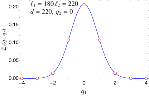
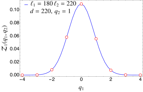
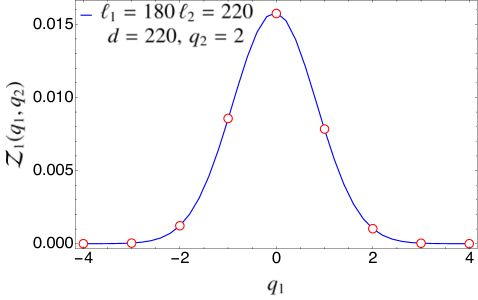
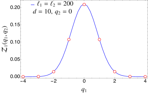
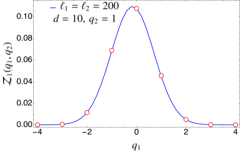
In Fig. 3, we compare the expression for found in Eq. (94) for the case of disjoint intervals with the exact numerical results obtained for the tight-binding model using the methods of Appendix A. The agreement is excellent. We remark that in Fig. 3 there is no free parameter when matching the analytical prediction with the numerical data since we know the expression of the non-universal constants for this particular system. In Fig. 4, we have repeated the same analysis in the case of adjacent intervals (), checking the validity of Eq. (97).

5.2 Symmetry-resolved mutual information
We compute now the symmetry-resolved mutual information defined in Eq. (8). We need the probability derived in Eq. (100) as well as the symmetry-resolved entropies for and its parts and separately. For the entropies of and , we can use the results for a single interval obtained in Ref. riccarda while, for the full subsystem , it can be derived from the Fourier transform of the charged moments determined in Eq. (99) by applying Eq. (13). The three symmetry-resolved entropies can eventually be written in the form
| (102) |
where is the total entanglement entropy of subsystem . In this expression, when , we have to take and while, if , then and . The auxiliary quantities and in Eq. (102) are defined in terms of as
| (103) |
For the tight-binding model, we know the explicit value of these non-universal constants,
| (104) |
From Eqs. (100) and (102), we can now obtain an explicit expression for the symmetry-resolved mutual information. Since the conditional probability satisfies Eq. (101), we have
| (105) | |||||
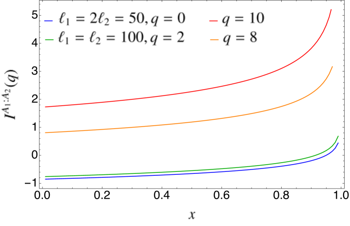
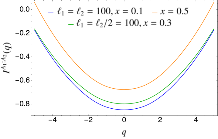
where is the total mutual information of Eq. (3) and we have introduced the rescaled subsystem length . We plot this function in Fig. 5. As we anticipated, the symmetry-resolved mutual information is not a good measure of the total correlations between and in each symmetry sector since it can assume negative values.
Finally, we can also derive the number mutual information defined in Eq. (10). Applying in that formula the result for obtained in Eq. (105), we have
| (106) | |||||
Since and
| (107) |
then Eq. (5.2) becomes
| (108) |
In the limit , this expression behaves as
| (109) |
This result resembles the one for the number entropy of a single interval (see e.g. riccarda ), where a double logarithmic correction in the subsystem length also appears, even though, in our case, the dependence on the parameters is more involved. On the other hand, it is a simple function of the Luttinger parameter since, as we already pointed out, the only effect of in the Gaussian factor of the Fourier transform of the multi-charged moments is renormalising its variance.
6 Conclusions
In this manuscript, we have computed the multi-charged moments of two intervals in the ground state of the free massless Dirac field and the massless compact boson, with arbitrary compactification radius. Using the replica approach, the multi-charged moments are given by the partition function of the theory on a higher genus Riemann surface with a different magnetic flux inserted in each interval. We have carried out the analysis of such partition function for the two CFTs under investigation in full generality, allowing the background magnetic flux to generate a different twisted boundary condition at each end-point of the intervals. In the case of the Dirac field, we have adapted the diagonalisation in the replica space method of Ref. CFH , to account for the different monodromy of the fields at each end-point. In the compact boson theory, we have chosen a geometric approach, and we have directly considered the four-point correlator on the Riemann surface of the vertex operators that implement the flux. It turns out that the known formulae for such correlator diverge in our case Verlinde . Once we properly regularised them, we have obtained a cumbersome expression for the multi-charged moments in terms of Riemann-Siegel Theta functions. Nevertheless, we have found several remarkable identities concerning the prime forms of the Riemann surface that allow to dramatically simplify the final result for the multi-charged moments. The factor due to the magnetic fluxes is eventually an algebraic function of the lengths of the intervals and their separation—identical to the one obtained in the Dirac theory. In fact, for a certain value of the compactification radius, the multi-charged moments of both theories are equal, generalising the known identity between their two-interval Rényi entropies HLM13 .
Given the simple expression obtained for the multi-charged moments, we can easily calculate their Fourier transform, which has a Gaussian form. From it, we have finally derived formulae for several interesting quantities such as the joint probability distribution of the charge for simultaneous measures in the two intervals, the symmetry-resolved mutual information pbc-21 and the number mutual information.
Let us conclude this manuscript discussing few outlooks. The multi-charged moments analysed here can be used to study the symmetry decomposition of the negativity in imbalance sectors goldstein1 . This is a measure of entanglement in mixed states which involves the partial transposition of the reduced density matrix. In the replica approach, this operation can be performed by properly fixing the different fluxes and exchanging the end-points of the transposed interval. A further generalisation is to identify the holographic dual of the multi-charged moments, which would be the starting point to compute the symmetry-resolved mutual information in the AdS/CFT correspondence, as done for the entanglement entropy in Ref. znm-20 . Partition functions with twisted boundary conditions, as the ones considered here, have been also proposed as non-local order parameters to distinguish various topological phases of spin chains ssr1-17 ; ssr-16 . We think that our analysis for the multi-charged moments can be useful to make progresses also in that direction. Finally, even though far beyond the scope of this manuscript, it would be interesting to obtain a rigorous proof of the identities for the prime forms that we have found and numerically checked here.
Acknowledgments
We thank Benoit Estienne, Yacine Ikhlef and Tamara Grava for useful discussions. PC, FA and SM acknowledge support from ERC under Consolidator grant number 771536 (NEMO).
Appendices
Appendix A Numerical Methods
For the numerical test of our field theory results, we consider the following lattice discretisation of the Dirac fermion, known as tight-binding model,
| (110) |
where and are fermionic creation and annihilation operators that satisfy the anti-commutation relations . In terms of them, the charge operator reads
| (111) |
The two-point correlation functions in the ground state of Eq. (110) are of the form
| (112) |
and, due to the particle number conservation, . As well-known p-03 ; pe-09 , the moments can be calculated from the restriction of the two-point correlation matrix to the subsystem , that is , with . The charged moments can also be easily computed numerically in terms of the matrix using the formula goldstein ; riccarda
| (113) |
where are the eigenvalues of and is the number of sites in the interval . In the case of the multi-charged moments defined in Eq. (14), the method used to compute can not be applied since does not commute with the charges and of the two parts of . Following Ref. pbc-21 (which was based on gec-18 ), we rewrite Eq. (14) as
| (114) |
where
| (115) |
Although is not a density matrix, it is a Gaussian operator with an associated two-point correlation matrix, , given by
| (116) |
Applying the rules for the composition of Gaussian operators fc-10 and introducing , we get pbc-21
| (117) |
where
| (118) |
and the notation , , refers to correlations between sites in and . This result allows to exactly compute the multi-charged moments in the tight-binding model for different values of and , as showed in Fig. 2. The Fourier transform of gives the quantities analysed in Fig. 3 and Fig. 4.
Appendix B Derivation of the normalised holomorphic differentials
In this Appendix, we present the detailed derivation of the expression given in Eq. (64) for the normalised holomorphic differentials of the Riemann surface . Recall that, according to Eq. (62), they are normalised with respect to the homology basis . In order to define this basis, it is convenient to introduce an auxiliary basis of non-contractible cycles, which we call and . The cycle encloses anticlockwise the branch cut in the -sheet of the surface. The dual cycle connects anticlockwise the and sheets through the branch cut and then it goes back to the sheet through the branch cut . In Fig. 6, we draw the auxiliary homology basis in the case . The cycles and are defined in terms of the auxiliary ones by
| (119) |
with and .
We can now obtain by following the usual procedure considered in the literature, see e.g. Enolskii ; Enolskii2 . We first take the basis of canonical holomorphic differentials of the surface ,
| (120) |
If we denote by and the matrices with entries
| (121) |
then the normalised holomorphic differentials can be calculated from such that
| (122) |
where are the entries of the inverse of the matrix . Furthermore, by combining Eq. (63) with Eqs. (121) and (122), the matrix of periods in Eq. (56) can be obtained from
| (123) |
To compute the matrices and , it is useful to consider the auxiliary homology basis .
The advantage of taking this basis is that it is easier to calculate the contour integrals of along the cycles and than along and . In fact, let us denote by and the matrices analogous to and but integrating now along the auxiliary cycles and respectively,
| (124) |
Then, by taking the correct branches for , we find that
| (125) | |||||
and
| (126) | |||||
where we have employed the identities
| (127) |
If we apply now the relation of Eq. (119) between both homology basis, then we directly obtain the matrices ,
| (128) |
and
| (129) | |||||
Appendix C Prime form identities
The identities for the regularised prime forms of Eqs.(83)-(86) can be easily proved when (genus one). In that case, the matrix of periods of Eq. (56) is a scalar and the Theta function that appears in Eq. (81) reduces to a Jacobi theta function, . The images under the Abel-Jacobi map in Eqs. (68)-(70) are in this case
| (131) |
Here we illustrate the proof of Eq. (84). The rest of identities can be checked in a similar way by applying the different relations in Sec. 20.2 of Ref. nist . If , Eq. (81) takes the following form for , ,
| (132) |
where is defined below Eq. (57). If we apply the half-period translation , the equality
| (133) |
and the relation between the hypergeometric function and the Jacobi theta function , we find
| (134) |
Finally, employing the well-known equality
| (135) |
we obtain Eq. (84).
The results for led us to conjecture the generalisation of Eqs. (83)-(86) for higher genus. Unfortunately, we have not been able to find a proof for them, although they can be tested numerically with great accuracy, as we show in Fig. 7. The dots are the result of evaluating numerically the definition in Eq. (81) of , while the solid lines are the functions on the right hand side of the identities in Eqs. (83)-(86).
References
- (1) M. A. Nielsen and I. L. Chuang, Quantum computation and quantum information, Cambridge University Press, Cambridge, UK, 10th anniversary ed. (2010).
- (2) T. Nishioka, S. Ryu, and T. Takayanagi, Holographic entanglement entropy: an overview, J. Phys. A 42, 504008 (2009).
- (3) M. Rangamani and T. Takanayagi, Holographic Entanglement Entropy, Lect. Notes Phys. 931 (2017).
- (4) L. Amico, R. Fazio, A. Osterloh, and V. Vedral, Entanglement in many-body systems, Rev. Mod. Phys. 80, 517 (2008).
- (5) P. Calabrese, J. Cardy, and B. Doyon, Entanglement entropy in extended quantum systems, J. Phys. A 42, 500301 (2009).
- (6) J. Eisert, M. Cramer, and M. B. Plenio, Area laws for the entanglement entropy, Rev. Mod. Phys. 82, 277 (2010).
- (7) N. Laflorencie, Quantum entanglement in condensed matter systems, Phys. Rep. 643, 1 (2016).
- (8) C. G. Callan and F. Wilczek, On Geometric Entropy, Phys. Lett. B 333, 55 (1994).
- (9) C. Holzhey, F. Larsen, and F. Wilczek, Geometric and renormalized entropy in conformal field theory, Nucl. Phys. B 424, 443 (1994).
- (10) P. Calabrese and J. Cardy, Entanglement entropy and quantum field theory, J. Stat. Mech. (2004) P06002.
- (11) P. Calabrese and J. Cardy, Entanglement entropy and conformal field theory, J. Phys. A 42, 504005 (2009).
- (12) M. Caraglio and F. Gliozzi, Entanglement entropy and twist fields, JHEP 11 (2008) 076.
- (13) S. Furukawa, V. Pasquier, and J. Shiraishi, Mutual Information and Boson Radius in Critical Systems in One Dimension, Phys. Rev. Lett. 102, 170602 (2009).
- (14) P. Calabrese, J. Cardy, and E. Tonni, Entanglement entropy of two disjoint intervals in conformal field theory, J. Stat. Mech. (2009) P11001.
- (15) P. Calabrese, J. Cardy, and E. Tonni, Entanglement entropy of two disjoint intervals in conformal field theory II, J. Stat. Mech. (2011) P01021.
- (16) P. Calabrese, J. Cardy, and E. Tonni, Entanglement negativity in quantum field theory, Phys. Rev. Lett. 109, 130502 (2012).
- (17) P. Calabrese, J. Cardy, and E. Tonni, Entanglement negativity in extended systems: a quantum field theory approach, J. Stat. Mech. (2013) P02008 .
- (18) P. Calabrese, L. Tagliacozzo, and E. Tonni, Entanglement negativity in the critical Ising chain, J. Stat. Mech. (2013) P05002.
- (19) V. Alba, Entanglement negativity and conformal field theory: a Monte Carlo study, J. Stat. Mech. (2013) P05013.
- (20) A. Coser, E. Tonni, and P. Calabrese, Towards the entanglement negativity of two disjoint intervals for a one dimensional free fermion, J. Stat. Mech. (2016) 033116.
- (21) F. Ares, R. Santachiara, and J. Viti, Crossing-symmetric Twist Field Correlators and Entanglement Negativity in Minimal CFTs, JHEP 10 (2021) 175.
- (22) G. Rockwood, Replicated Entanglement Negativity for Disjoint Intervals in the Ising and Free Compact Boson Conformal Field Theories, arXiv:2203.04339.
- (23) T. Dupic, B. Estienne, and Y. Ikhlef, Entanglement entropies of minimal models from null-vectors, SciPost Phys. 4, 031 (2018).
- (24) H. Casini, C. D. Fosco, and M. Huerta, Entanglement and alpha entropies for a massive Dirac field in two dimensions, J. Stat. Mech. (2005) P07007.
- (25) H. Casini and M. Huerta, Reduced density matrix and internal dynamics for multicomponent regions, Class. Quant. Grav. 26, 185005 (2009)
- (26) V. Alba, L. Tagliacozzo, and P. Calabrese, Entanglement entropy of two disjoint blocks in critical Ising models, Phys. Rev. B 81, 060411(R) (2010).
- (27) V. Alba, L. Tagliacozzo, and P. Calabrese, Entanglement entropy of two disjoint intervals in theories, J. Stat. Mech. (2011) P06012.
- (28) M. A. Rajabpour and F. Gliozzi, Entanglement entropy of two disjoint intervals from fusion algebra of twist fields, J. Stat. Mech. (2012) P02016.
- (29) M. Headrick, A. Lawrence, and M. Roberts, Bose-Fermi duality and entanglement entropies, J. Stat. Mech. (2013) P02022.
- (30) A. Coser, L. Tagliacozzo, and E. Tonni, On Rényi entropies of disjoint intervals in conformal field theory, J. Stat. Mech. (2014) P01008.
- (31) C. De Nobili, A. Coser, and E. Tonni, Entanglement entropy and negativity of disjoint intervals in CFT: some numerical extrapolations, J. Stat. Mech. (2015) P06021.
- (32) A. Coser, E. Tonni, and P. Calabrese, Spin structures and entanglement of two disjoint intervals in conformal field theories, J. Stat. Mech. (2016) 053109.
- (33) P. Ruggiero, E. Tonni, and P. Calabrese, Entanglement entropy of two disjoint intervals and the recursion formula for conformal blocks, J. Stat. Mech. (2018) 113101.
- (34) A. Bastianello, Rényi entanglement entropies for the compactified massless boson with open boundary conditions, JHEP 10 (2019) 141.
- (35) A. Bastianello, J. Dubail, and J.M. Stéphan, Entanglement entropies of inhomogeneous Luttinger liquids, J. Phys. A: Math. Theor. 53, 155001 (2020).
- (36) T. Grava, A. P. Kels, and E. Tonni, Entanglement of Two Disjoint Intervals in Conformal Field Theory and the 2D Coulomb Gas on a Lattice, Phys. Rev. Lett. 127, 141605 (2021).
- (37) M. Gerbershagen, Monodromy methods for torus conformal blocks and entanglement entropy at large central charge, JHEP 08 (2021) 143.
- (38) N. Laflorencie and S. Rachel, Spin-resolved entanglement spectroscopy of critical spin chains and Luttinger liquids, J. Stat. Mech. (2014) P11013.
- (39) M. Goldstein and E. Sela, Symmetry-Resolved Entanglement in Many-Body Systems, Phys. Rev. Lett. 120, 200602 (2018).
- (40) J. C. Xavier, F. C. Alcaraz, and G. Sierra, Equipartition of the entanglement entropy, Phys. Rev. B 98, 041106 (2018).
- (41) A. Lukin, M. Rispoli, R. Schittko, M. E. Tai, A. M. Kaufman, S. Choi, V. Khemani, J. Leonard, and M. Greiner, Probing entanglement in a many-body localized system, Science 364, 256 (2019).
- (42) D. Azses, R. Haenel, Y. Naveh, R. Raussendorf, E. Sela, and E. G. Dalla Torre, Identification of Symmetry-Protected Topological States on Noisy Quantum Computers, Phys. Rev. Lett. 125, 120502 (2020).
- (43) A. Neven, J. Carrasco, V. Vitale, C. Kokail, A. Elben, M. Dalmonte, P. Calabrese, P. Zoller, B. Vermersch, R. Kueng, and B. Kraus, Symmetry-resolved entanglement detection using partial transpose moments, Npj Quantum Inf. 7, 152 (2021).
- (44) V. Vitale, A. Elben, R. Kueng, A. Neven, J. Carrasco, B. Kraus, P. Zoller, P. Calabrese, B. Vermersch, and M. Dalmonte, Symmetry-resolved dynamical purification in synthetic quantum matter, SciPost Phys. 12, 106 (2022).
- (45) R. Bonsignori, P. Ruggiero, and P. Calabrese, Symmetry resolved entanglement in free fermionic systems, J. Phys. A 52, 475302 (2019).
- (46) S. Fraenkel and M. Goldstein, Symmetry resolved entanglement: Exact results in 1d and beyond, J. Stat. Mech. (2020) 033106.
- (47) N. Feldman and M. Goldstein, Dynamics of Charge-Resolved Entanglement after a Local Quench, Phys. Rev. B 100, 235146 (2019).
- (48) S. Murciano, G. Di Giulio, and P. Calabrese, Symmetry resolved entanglement in gapped integrable systems: a corner transfer matrix approach, SciPost Phys. 8, 046 (2020).
- (49) P. Calabrese, M. Collura, G. Di Giulio, and S. Murciano, Full counting statistics in the gapped XXZ spin chain, EPL 129, 60007 (2020).
- (50) H. M. Wiseman and J. A. Vaccaro, Entanglement of Indistinguishable Particles Shared between Two Parties, Phys. Rev. Lett. 91, 097902 (2003).
- (51) H. Barghathi, C. M. Herdman, and A. Del Maestro, Rényi Generalization of the Accessible Entanglement Entropy, Phys. Rev. Lett. 121, 150501 (2018).
- (52) H. Barghathi, E. Casiano-Diaz, and A. Del Maestro, Operationally accessible entanglement of one dimensional spinless fermions, Phys. Rev. A 100, 022324 (2019).
- (53) H. Barghathi, J. Yu, and A. Del Maestro Theory of noninteracting fermions and bosons in the canonical ensemble, Phys. Rev. Res. 2, 043206 (2020).
- (54) S. Murciano, P. Ruggiero, and P. Calabrese, Symmetry resolved entanglement in two-dimensional systems via dimensional reduction, J. Stat. Mech. (2020) 083102.
- (55) M. T. Tan and S. Ryu, Particle Number Fluctuations, Rényi and Symmetry-resolved Entanglement Entropy in Two-dimensional Fermi Gas from Multi-dimensional bosonisation, Phys. Rev. B 101, 235169 (2020).
- (56) Z. Ma, C. Han, Y. Meir, and E. Sela, Symmetric inseparability and number entanglement in charge conserving mixed states, Phys. Rev. A 105, 042416 (2022).
- (57) F. Ares, S. Murciano, and P. Calabrese, Symmetry-resolved entanglement in a long-range free-fermion chain, J. Stat. Mech. (2022) 063104.
- (58) N. G. Jones, Symmetry-resolved entanglement entropy in critical free-fermion chains, J. Statist. Phys. 188 (2022) 28.
- (59) L. Piroli, E. Vernier, M. Collura, and P. Calabrese, Thermodynamic symmetry resolved entanglement entropies in integrable systems, J. Stat. Mech. (2022) 073102.
- (60) S. Murciano, G. Di Giulio, and P. Calabrese, Entanglement and symmetry resolution in two dimensional free quantum field theories, JHEP 08 (2020) 073.
- (61) D. X. Horvath, L. Capizzi, and P. Calabrese, U(1) symmetry resolved entanglement in free 1+1 dimensional field theories via form factor bootstrap, JHEP 05 (2021) 197.
- (62) D. X. Horvath, P. Calabrese, and O. A. Castro-Alvaredo, Branch Point Twist Field Form Factors in the sine-Gordon Model II: Composite Twist Fields and Symmetry Resolved Entanglement, SciPost Phys. 12, 088 (2022).
- (63) D. X. Horvath and P. Calabrese, Symmetry resolved entanglement in integrable field theories via form factor bootstrap, JHEP 11 (2020) 131.
- (64) L. Capizzi, D. X. Horvath, P. Calabrese, and O. A. Castro-Alvaredo, Entanglement of the 3-State Potts Model via Form Factor Bootstrap: Total and Symmetry Resolved Entropies, JHEP 05 (2022) 113.
- (65) E. Cornfeld, M. Goldstein, and E. Sela, Imbalance Entanglement: Symmetry Decomposition of Negativity, Phys. Rev. A 98, 032302 (2018).
- (66) L. Capizzi, P. Ruggiero, and P. Calabrese, Symmetry resolved entanglement entropy of excited states in a CFT, J. Stat. Mech. (2020) 073101.
- (67) S. Murciano, R. Bonsignori, and P. Calabrese, Symmetry decomposition of negativity of massless free fermions, SciPost Phys. 10, 111 (2021).
- (68) H.-H. Chen, Symmetry decomposition of relative entropies in conformal field theory, JHEP 07 (2021) 084.
- (69) L. Capizzi and P. Calabrese, Symmetry resolved relative entropies and distances in conformal field theory, JHEP 10 (2021) 195.
- (70) L. Hung and G. Wong, Entanglement branes and factorization in conformal field theory, Phys. Rev. D 104, 026012 (2021).
- (71) P. Calabrese, J. Dubail, and S. Murciano, Symmetry-resolved entanglement entropy in Wess-Zumino-Witten models, JHEP 10 (2021) 067.
- (72) R. Bonsignori and P. Calabrese, Boundary effects on symmetry resolved entanglement, J. Phys. A 54, 015005 (2021).
- (73) B. Estienne, Y. Ikhlef, and A. Morin-Duchesne, Finite-size corrections in critical symmetry-resolved entanglement, SciPost Phys. 10, 054 (2021).
- (74) H.-H. Chen, Charged Rényi negativity of massless free bosons, JHEP 02 (2022) 117.
- (75) A. Milekhin and A. Tajdini, Charge fluctuation entropy of Hawking radiation: a replica-free way to find large entropy, arXiv:2109.03841.
- (76) M. Ghasemi, Universal Thermal Corrections to Symmetry-Resolved Entanglement Entropy and Full Counting Statistics, arXiv:2203.06708.
- (77) S. Zhao, C. Northe, and R. Meyer, Symmetry-Resolved Entanglement in AdS3/CFT2 coupled to Chern-Simons Theory, JHEP 07 (2021) 030.
- (78) K. Weisenberger, S. Zhao, C. Northe, and R. Meyer, Symmetry-resolved entanglement for excited states and two entangling intervals in AdS3/CFT2, JHEP 12 (2021) 104.
- (79) S. Zhao, C. Northe, K. Weisenberger, and R. Meyer, Charged Moments in Higher Spin Holography, JHEP 05 (2022) 166.
- (80) S. Baiguera, L. Bianchi, S. Chapman, and D. A. Galante, Shape Deformations of Charged Rényi Entropies from Holography, JHEP 06 (2022) 068.
- (81) G. Parez, R. Bonsignori, and P. Calabrese, Quasiparticle dynamics of symmetry resolved entanglement after a quench: the examples of conformal field theories and free fermions, Phys. Rev. B 103, L041104 (2021).
- (82) G. Parez, R. Bonsignori, and P. Calabrese, Exact quench dynamics of symmetry resolved entanglement in a free fermion chain, J. Stat. Mech. (2021) 093102.
- (83) S. Fraenkel and M. Goldstein, Entanglement Measures in a Nonequilibrium Steady State: Exact Results in One Dimension, SciPost Phys. 11, 085 (2021).
- (84) G. Parez, R. Bonsignori, and P. Calabrese, Dynamics of charge-imbalance-resolved entanglement negativity after a quench in a free-fermion mode, J. Stat. Mech. (2022) 053103.
- (85) S. Scopa and D. X. Horvath, Exact hydrodynamic description of symmetry-resolved Rényi entropies after a quantum quench, J. Stat. Mech. (2022) 083104.
- (86) H.-H. Chen, Dynamics of charge imbalance resolved negativity after a global quench in free scalar field theory, JHEP 08 (2022) 146.
- (87) X. Turkeshi, P. Ruggiero, V. Alba, and P. Calabrese, Entanglement equipartition in critical random spin chains, Phys. Rev. B 102, 014455 (2020).
- (88) M. Kiefer-Emmanouilidis, R. Unanyan, J. Sirker, and M. Fleischhauer, Bounds on the entanglement entropy by the number entropy in non-interacting fermionic systems, SciPost Phys 8, 083 (2020).
- (89) M. Kiefer-Emmanouilidis, R. Unanyan, J. Sirker, and M. Fleischhauer, Evidence for unbounded growth of the number entropy in many-body localized phases, Phys. Rev. Lett. 124, 243601 (2020).
- (90) M. Kiefer-Emmanouilidis, R. Unanyan, M. Fleischhauer, and J. Sirker, Absence of true localization in many-body localized phases, Phys. Rev. B 103, 024203 (2021).
- (91) E. Cornfeld, L. A. Landau, K. Shtengel, and E. Sela, Entanglement spectroscopy of non-Abelian anyons: Reading off quantum dimensions of individual anyons, Phys. Rev. B 99, 115429 (2019).
- (92) K. Monkman and J. Sirker, Operational Entanglement of Symmetry-Protected Topological Edge States, Phys. Rev. Res. 2, 043191 (2020).
- (93) D. Azses and E. Sela, Symmetry resolved entanglement in symmetry protected topological phases, Phys. Rev. B 102, 235157 (2020).
- (94) D. Azses, R. Haenel, Y. Naveh, R. Raussendorf, E. Sela, and E. G. Dalla Torre, Identification of Symmetry-Protected Topological States on Noisy Quantum Computers, Phys. Rev. Lett. 125, 120502 (2020).
- (95) D. Azses, E. G. Dalla Torre, and E. Sela, Observing Floquet topological order by symmetry resolution, Phys. Rev. B 104, L220301 (2021).
- (96) B. Oblak, N. Regnault, and B. Estienne, Equipartition of Entanglement in Quantum Hall States, Phys. Rev. B 105, 115131 (2022).
- (97) A. Belin, L.-Y. Hung, A. Maloney, S. Matsuura, R. C. Myers, and T. Sierens, Holographic charged Rényi entropies, JHEP 12 (2013) 059.
- (98) P. Caputa, G. Mandal, and R. Sinha, Dynamical entanglement entropy with angular momentum and charge, JHEP 11 (2013) 052.
- (99) P. Caputa, M. Nozaki, and T. Numasawa, Charged Entanglement Entropy of Local Operators, Phys. Rev. D 93, 105032 (2016).
- (100) J. S. Dowker, Conformal weights of charged Rényi entropy twist operators for free scalar fields in arbitrary dimensions, J. Phys. A 49, 145401 (2016).
- (101) J. S. Dowker, Charged Rényi entropies for free scalar fields, J. Phys. A 50, 165401 (2017).
- (102) H. Shapourian, K. Shiozaki, and S. Ryu, Partial time-reversal transformation and entanglement negativity in fermionic systems, Phys. Rev. B 95, 165101 (2017).
- (103) H. Shapourian, P. Ruggiero, S. Ryu, and P. Calabrese, Twisted and untwisted negativity spectrum of free fermions, SciPost Phys. 7, 037 (2019).
- (104) H. Shapourian, K. Shiozaki, and S. Ryu, Many-Body Topological Invariants for Fermionic Symmetry-Protected Topological Phases, Phys. Rev. Lett. 118, 216402 (2017).
- (105) K. Shiozaki, H. Shapourian, and S. Ryu, Many-body topological invariants in fermionic symmetry protected topological phases: Cases of point group symmetries, Phys. Rev. B 95, 205139 (2017).
- (106) M. Kiefer-Emmanouilidis, R. Unanyan, M. Fleischhauer, and J. Sirker, Slow delocalization of particles in many-body localized phases, Phys. Rev. B 103, 024203 (2021).
- (107) Y. Zhao, D. Feng, Y. Hu, S. Guo, and J. Sirker, Entanglement dynamics in the three-dimensional Anderson model, Phys. Rev. B 102, 195132 (2020).
- (108) M. Kiefer-Emmanouilidis, R. Unanyan, M. Fleischhauer, and J. Sirker, Unlimited growth of particle fluctuations in many-body localized phases, Ann. Phys. 168481 (2021).
- (109) J. L. Cardy, O. A. Castro-Alvaredo, and B. Doyon, Form factors of branch-point twist fields in quantum integrable models and entanglement entropy, J. Stat. Phys. 130, 129 (2008).
- (110) V. Knizhnik, Analytic fields on Riemann surfaces. II, Comm. Math. Phys. 112, 567 (1987).
- (111) L. J. Dixon, D. Friedan, E. J. Martinec, and S. H. Shenker, The Conformal Field Theory Of Orbifolds, Nucl. Phys. B 282, 13 (1987).
- (112) B.-Q. Jin and V. E. Korepin, Quantum spin chain, Toeplitz determinants and Fisher-Hartwig conjecture, J. Stat. Phys. 116, 79 (2004).
- (113) P. Di Francesco, P. Mathieu, and D. Senechal, Conformal Field Theory, Springer-Verlag, New York, (1997).
- (114) J. D. Fay, Theta functions on Riemann surfaces, Springer Notes in Mathematics 352 (Springer, 1973).
- (115) E. Verlinde and H. Verlinde, Chiral Bosonization, Determinants and the String Partition Function, Nucl. Phys. B, 288, 357 (1987).
- (116) S. Groha, F. H. L. Essler, and P. Calabrese, Full Counting Statistics in the Transverse Field Ising Chain, SciPost Phys. 4, 043 (2018).
- (117) V. Enolskii and T. Grava, Singular curves, Riemann-Hilbert problem and modular solutions of the Schlesinger equation, Int. Math. Res. Not. 32, 1619 (2004).
- (118) V. Enolskii and T. Grava, Thomae type formulae for singular curves, Lett. Math. Phys. 76, 187 (2006).
- (119) I. Peschel, Calculation of reduced density matrices from correlation functions, J. Phys. A 36, L205 (2003).
- (120) I. Peschel and V. Eisler, Reduced density matrices and entanglement entropy in free lattice models, J. Phys. A 42, 504003 (2009).
- (121) M. Fagotti and P. Calabrese, Entanglement entropy of two disjoint blocks in XY chains, J. Stat. Mech. (2010) P04016.
- (122) F. W. J. Olver, A. B. Olde Daalhuis, D. W. Lozier, B. I. Schneider, R. F. Boisvert, C. W. Clark, B. R. Miller, and B. V. Saunders (ed), NIST Digital Library of Mathematical Functions, (Gaithersburg: National Institute of Standards and Technology) (http://dlmf.nist.gov/).