Multi-horizons black hole solutions, photon sphere and perihelion shift
in weak ghost-free Gauss-Bonnet theory of gravity

G. G. L. Nashed nashed@bue.edu.eg Centre for Theoretical Physics, The British University in Egypt, P.O. Box 43, El Sherouk City, Cairo 11837, Egypt Shin’ichi Nojiri nojiri@gravity.phys.nagoya-u.ac.jp Department of Physics, Nagoya University, Nagoya 464-8602, Japan
&
Kobayashi-Maskawa Institute for the Origin of Particles and the Universe, Nagoya University, Nagoya 464-8602, Japan

Abstract

Among the modified gravitational theories, the ghost-free Gauss-Bonnet (GFGB) theory of gravity has been considered from the viewpoint of cosmology. The best way to check its applicability could be to elicit observable predicts which give guidelines or limitations on the theory, which could be contrasted with the actual observations. In the present study, we derive consistent field equations for GFGB and by applying the equations to a spherically symmetric space-time, we obtain new spherically symmetric black hole (BH) solutions. We study the physical properties of these BH solutions and show that the obtained space-time possesses multi-horizons and the Gauss-Bonnet invariants in the space-time are not trivial. We also investigate the thermodynamical quantities related to these BH solutions and we show that these quantities are consistent with what is known in the previous works. Finally, we study the geodesic equations of these solutions which give the photon spheres and we find the perihelion shift for weak GFGB. In addition, we calculate the first-order GFGB perturbations in the Schwarzschild solution and new BH solutions and show that we improve and extend existing results in the past literature on the spherically symmetric solutions.

pacs:

95.35.+d, 98.80.-k, 98.80.Cq, 95.36.+x

I Introduction

Although more than one hundred years have passed after the construction of Einstein’s theory of general relativity (GR), GR is still the most established macroscopic theory of gravity that is widely accepted. In spite of its vast success in both weak and strong couplings Will:2014kxa ; Ishak:2018his , however, there is still no harmonic way to link the macroscopic theory of GR to a quantum field theory. Moreover, GR predicts space-time singularity which has mathematical results in its construction. The problem of singularity leads scientists to search for other theories of gravity that could coincide with GR in the scale of daily life and/or the scale of the solar system. It is interesting to note that Lovelock’s theory Lovelock:1971yv has explained that in four dimensions, Einsteins GR is the unique metric theory of gravity that could yields symmetric, covariant second-order field equations. Therefore, one of the attempts to amend Einstein’s GR is to work in space-times with extra dimensions Clifton:2011jh . In these attempts, the most general set of theories could be the Lovelock theories which yield symmetric, covariant second-order field equations regarding the metric tensor in any space-time dimensions Padmanabhan:2013xyr . The Lagrangian of the Lovelock theory is given as follows,

\displaystyle\mathcal{L}=\sqrt{-g}\left(-2\Lambda+R+\alpha\mathcal{G}+\cdots\right)\,,

(1)

with $\mathcal{G}\equiv R^{2}-4R_{\mu\nu}R^{\mu\nu}+R_{\alpha\beta\mu\nu}R^{\alpha\beta\mu\nu}$ being the Gauss-Bonnet (GB) invariant which yields the first order correction to the action of Einstein’s theory with a cosmological constant $\Lambda$ . Although the GB invariant yields nontrivial effects when the space-time dimensions are larger than four, the invariant is topological in four dimensions 10.2307/1969203 . Regardless of being quadratic in curvatures, the GB invariant has theoretical wide advantages from the viewpoints of string theory Ferrara:1996hh ; Antoniadis:1997eg ; Zwiebach:1985uq ; Nepomechie:1985us ; Callan:1986jb ; Candelas:1985en ; Gross:1986mw .

Many researchers have been tempted by the idea of harmony merging the effect of the GB invariant in a four-dimensional theory of gravity, which could yield equations of motions different from GR, avoiding Lovelock’s theorem. Glavan and Lin Glavan:2019inb have investigated the idea to rescale the GB coupling constant $\gamma$ in $N$ dimensions as $\gamma\rightarrow\gamma/(N-4)$ , so that there remains the contribution from the GB invariant in the limit $N\to 4$ . After that, there have appeared works, where spherical black hole solutionsKumar:2020uyz ; Fernandes:2020rpa ; Kumar:2020owy ; Ghosh:2020syx , the construction of cosmological solutions Li:2020tlo ; Kobayashi:2020wqy , the radiation of black holes and the collapse to the black hole Ghosh:2020vpc ; Shirafuji:1996im ; Malafarina:2020pvl , star-like objects Doneva:2020ped , the extension to more higher-curvature Lovelock theories Konoplya:2020qqh , the thermodynamical behavior of black hole solutions EslamPanah:2020hoj ; HosseiniMansoori:2020yfj ; Konoplya:2020cbv ; Hegde:2020xlv , and the physical properties of such objects Guo:2020zmf ; Konoplya:2020qqh ; Zhang:2020qew ; Roy:2020dyy ; NaveenaKumara:2020kpz ; Liu:2020vkh ; Heydari-Fard:2021ljh ; Kumar:2020sag ; Nashed:2018efg ; Islam:2020xmy ; Mishra:2020gce ; Devi:2020uac ; Churilova:2020mif have been investigated . In spite of all of these researches, the regularization method used in the four-dimensional Einstein-GB theory Glavan:2019inb has been shown to be inconsistent for many reasons Gurses:2020ofy ; Gurses:2020rxb ; Arrechea:2020evj ; Arrechea:2020gjw ; Bonifacio:2020vbk ; Nashed:2018cth ; Ai:2020peo ; Mahapatra:2020rds ; Nashed:2010ocg ; Hohmann:2020cor ; Cao:2021nng , which yield to the construction of different models of the regularized (harmonic) four-dimensional Einstein GB theories Lu:2020iav ; Kobayashi:2020wqy ; Fernandes:2020nbq ; Hennigar:2020lsl ; Aoki:2020lig ; Fernandes:2021dsb .

Due to several reasons, some researchers are suspicious about the procedure proposed in Glavan:2019inb . One reason is that the field equations of the Einstein-GB theory defined in higher dimensions can be divided into two various sets. One set yields the field equations which always come from higher dimensional theories and this set makes the specific action in the limit of $N\to 4$ non-trivial Gurses:2020ofy ; Gurses:2020rxb ; Arrechea:2020evj ; Nashed:2007cu ; Arrechea:2020gjw ; Mahapatra:2020rds . The tree-level graviton scattering amplitude was also investigated in this frame, apart from the Lagrangian, and it turned out that the dimensional continuation, $N\to 4$ , does not make the GB amplitude create any new four-dimensional GB gravitational amplitude Lin:2020kqe . All of these attempts yield the fact that the existence of the solution in the limit of $N\to 4$ does not mean that there is a four-dimensional theory as proposed in Glavan:2019inb . In spite of this situation, it could be important to mention that the field equations different from the four-dimensional Einstein GB gravity Lu:2020iav ; Kobayashi:2020wqy ; Fernandes:2020nbq ; Hennigar:2020lsl ; Aoki:2020lig support the same static spherically symmetric BH solution as constructed in Glavan:2019inb . Following the $N\to 4$ regularization of the scalar and vector type gravitational perturbation of the $N>4$ Einstein-GB BH Takahashi:2010gz ; Takahashi:2010ye , it has been investigated that the asymptotically flat or AdS/dS BHs are unstable for large positive values of the GB coupling parameter Konoplya:2020bxa ; Konoplya:2020juj . The quasinormal modes of the four-dimensional Einstein GB BH in the asymptotically AdS/dS space-time due to scalar, electromagnetic, and Dirac perturbations have been investigated in Devi:2020uac ; Churilova:2020mif . The quasi-bound states of massless scalar, electromagnetic, and Dirac fields in the asymptotically flat four-dimensional Einstein GB BH and the associated stability issue have been studied in Vieira:2021doo .

Because of the significance of the theories involving the GB scalar, which are encouraged by string theories in many cases, in this study, we shall briefly discuss the drawback of these theories, specifically the existence of ghosts. Generally, higher-derivative gravitational theories involve ghost degrees of freedom due to the Ostrogradskya’s instability Woodard:2015zca . It was explained in DeFelice:2009ak , that ghost degrees of freedom could happen at different levels of the theory, despite the cosmological perturbations level of $f(R,\mathcal{G})$ theories. It is the aim of the present study to derive the spherically symmetric BH solutions in the ghost-free $f\left(\mathcal{G}\right)$ gravitational theory proposed in Nojiri:2018ouv ; Nojiri:2021mxf .

This paper is organized as follows: In Section II, we present the basic tools for the ghost-free $f\left(\mathcal{G}\right)$ gravitational theory that is capable to describe the formulation of BH horizons. In Section III, we apply the field equations of GFGB to the spherically symmetric space-time and derive BH solutions with multi-horizons. In Section IV, we study the relevant physics of the BH solutions derived in Section III by showing their asymptote at $r\to\infty$ . Moreover, we show that by studying the thermodynamical behavior of these BH solutions by calculating their thermodynamical quantities like Hawking temperature, heat capacity, and the Gibbs free energy, we show that all these quantities related to the BHs derived in Section II are consistent with the results presented in the past literature. In Section V, we study the particle motion phenomenology for these BHs and derived their potential for the Schwarzschild background. Moreover, we derive the deviation from Einstein’s general relativity of the photon sphere and the perihelion shift. We close our study with the conclusion of the main results in Section VI.

Throughout the present study, we assume the relativistic units, i.e., $G=c=1$ .

II Brief summary of ghost-free $f(\mathcal{G})$ gravitational theory

In the present section, we will present briefly the ghost-free $f\left(\mathcal{G}\right)$ gravity in the formulation using the Lagrange multipliers. Moreover, we shall investigate how to obtain a ghost-free $f(\mathcal{G})$ gravity, and we shall employ the Lagrange multipliers formalism in order to achieve this. Before going to the details of the formalism, we will start the derivation by showing in detail how ghost modes could exist in $f\left(\mathcal{G}\right)$ gravity at the field equations level, and then construct the ghost-free model construction of the theory.

II.1 Ghosts in $f\left(\mathcal{G}\right)$ Gravity

Nojiri et al. Nojiri:2018ouv ; Nojiri:2021mxf have constructed a ghost-free $f\left(\mathcal{G}\right)$ gravity theory by using the Lagrange multiplier field. The original $f\left(\mathcal{G}\right)$ , whose action to has the following form,

\displaystyle S=\int d^{4}x\sqrt{-g}\left(\frac{1}{2\kappa^{2}}R+f\left(\mathcal{G}\right)+\mathcal{L}_{\mathrm{matter}}\right)\,,

(2)

have ghost as we show below. Here $\mathcal{L}_{\mathrm{matter}}$ is the Lagrangian density of the matters. The above action (2) can be rewritten as follows,

\displaystyle S=\int d^{4}x\sqrt{-g}\left(\frac{1}{2\kappa^{2}}R+h\left(\chi\right)\mathcal{G}-V\left(\chi\right)+\mathcal{L}_{\mathrm{matter}}\right)\,,

(3)

where $R$ is the Ricci scalar, $\chi$ is an auxiliary field, $\mathcal{G}$ is the GB invariant, $V(\chi)$ is the potential and $h(\chi)$ is a function of the auxiliary field. The variation of the action (3) w.r.t. the $\chi$ , gives,

\displaystyle 0=h^{\prime}\left(\chi\right)\mathcal{G}-V^{\prime}\left(\chi\right)\,.

(4)

Eq. (4) can be solved w.r.t. $\chi$ as a function of the GB invariant $\mathcal{G}$ , $\chi=\chi\left(\mathcal{G}\right)$ . Then by substituting the obtained expression of $\chi\left(\mathcal{G}\right)$ into Eq. (4), one can reobtain the action of Eq. (2) where $f\left(\mathcal{G}\right)$ is defined as,

\displaystyle f\left(\mathcal{G}\right)=h\left(\chi\left(\mathcal{G}\right)\right)\mathcal{G}-V\left(\chi\left(\mathcal{G}\right)\right)\,.

(5)

Furthermore, the varying of the action (4) w.r.t. the metric tensor yields:

\displaystyle 0=\frac{1}{2\kappa^{2}}\left(-R_{\mu\nu}+\frac{1}{2}g_{\mu\nu}R\right)+\frac{1}{2}T_{\mathrm{matter}\,\mu\nu}-\frac{1}{2}g_{\mu\nu}V\left(\chi\right)+D_{\mu\nu}^{\ \ \tau\eta}\nabla_{\tau}\nabla_{\eta}h\left(\chi\right)\,,

(6)

where the tensor $D_{\mu\nu}^{\ \ \tau\eta}$ is defined:

	$\displaystyle D_{\mu\nu}^{\ \ \tau\eta}\equiv$	$\displaystyle\,\left(\delta_{\mu}^{\ \tau}\delta_{\nu}^{\ \eta}+\delta_{\nu}^{\ \tau}\delta_{\mu}^{\ \eta}-2g_{\mu\nu}g^{\tau\eta}\right)R+\left(-4g^{\rho\tau}\delta_{\mu}^{\ \eta}\delta_{\nu}^{\ \sigma}-4g^{\rho\tau}\delta_{\nu}^{\ \eta}\delta_{\mu}^{\ \sigma}+4g_{\mu\nu}g^{\rho\tau}g^{\sigma\eta}\right)R_{\rho\sigma}$
		$\displaystyle\,+4R_{\mu\nu}g^{\tau\eta}-2R_{\rho\mu\sigma\nu}\left(g^{\rho\tau}g^{\sigma\eta}+g^{\rho\eta}g^{\sigma\tau}\right)\,.$		(7)

Since the auxiliary field $\chi$ can be rewritten as a function of the GB $\mathcal{G}$ , then Eq. (6) is a fourth order differential equation for the metric which may contain ghost modes.

In order to eliminate the ghost modes, we may add a canonical kinetic term of $\chi$ in the action (3)

\displaystyle S=\int d^{4}x\sqrt{-g}\left(\frac{1}{2\kappa^{2}}R+h\left(\chi\right)\mathcal{G}-\frac{1}{2}\partial_{\mu}\chi\partial^{\mu}\chi-V\left(\chi\right)+\mathcal{L}_{\mathrm{matter}}\right)\,,

(8)

where we have chosen the mass dimension of $\chi$ to be unity. Then variation of the action (8) w.r.t. $\chi$ and metric give Nojiri:2005vv ; Nojiri:2018ouv ; Nojiri:2021mxf ,

	$\displaystyle 0=$	$\displaystyle\Box\chi+h^{\prime}\left(\chi\right)\mathcal{G}-V^{\prime}\left(\chi\right)\,,$		(9)
	$\displaystyle 0=$	$\displaystyle\frac{1}{2\kappa^{2}}\left(-R_{\mu\nu}+\frac{1}{2}g_{\mu\nu}R\right)+\frac{1}{2}T_{\mathrm{matter}\,\mu\nu}+\frac{1}{2}\partial_{\mu}\chi\partial_{\nu}\chi-\frac{1}{2}g_{\mu\nu}\left(\frac{1}{2}\partial_{\rho}\chi\partial^{\rho}\chi+V\left(\chi\right)\right)+D_{\mu\nu}^{\ \ \tau\eta}\nabla_{\tau}\nabla_{\eta}h\left(\chi\right)\,.$		(10)

The equations derived in Eq. (9) do not have higher-order except the second-order derivatives which mean that we could not have ghosts.

The model (8), has a new dynamical degree of freedom, i.e., $\chi$ , however, if we like to minimize the dynamical degrees of freedom, we can insert a constraint as in the mimetic theory Chamseddine:2013kea ; Nojiri:2014zqa ; Dutta:2017fjw , by using the Lagrange multiplier field $\lambda$ , as follows,

\displaystyle S=\int d^{4}x\sqrt{-g}\left(\frac{1}{2\kappa^{2}}R+\lambda\left(\frac{1}{2}\partial_{\mu}\chi\partial^{\mu}\chi+\frac{\mu^{4}}{2}\right)-\frac{1}{2}\partial_{\mu}\chi\partial^{\mu}\chi+h\left(\chi\right)\mathcal{G}-V\left(\chi\right)+\mathcal{L}_{\mathrm{matter}}\right)\,,

(11)

where $\mu$ is a constant which has a mass dimension. Thus, by varying action (11) w.r.t. $\lambda$ , we obtain,

\displaystyle 0=\frac{1}{2}\partial_{\mu}\chi\partial^{\mu}\chi+\frac{\mu^{4}}{2}\,.

(12)

Because of the fact that the kinetic term becomes a constant, the kinetic term in Eq. (11) can be absorbed by using the redefinition of potential $V\left(\chi\right)$ ,

\displaystyle\tilde{V}\left(\chi\right)\equiv\frac{1}{2}\partial_{\mu}\chi\partial^{\mu}\chi+V\left(\chi\right)=-\frac{\mu^{4}}{2}+V\left(\chi\right)\,.

(13)

Now, the action of Eq. (11) can be rewritten as follows,

\displaystyle S=\int d^{4}x\sqrt{-g}\left(\frac{1}{2\kappa^{2}}R+\lambda\left(\frac{1}{2}\partial_{\mu}\chi\partial^{\mu}\chi+\frac{\mu^{4}}{2}\right)+h\left(\chi\right)\mathcal{G}-\tilde{V}\left(\chi\right)+\mathcal{L}_{\mathrm{matter}}\right)\,.

(14)

The action given in Eq. (14) yields, in addition to Eq. (12), the following two equations of motion,

	$\displaystyle 0=$	$\displaystyle-\frac{1}{\sqrt{-g}}\partial_{\mu}\left(\lambda\omega(\chi)g^{\mu\nu}\sqrt{-g}\partial_{\nu}\chi\right)+h^{\prime}\left(\chi\right)\mathcal{G}-{\tilde{V}}^{\prime}\left(\chi\right)+\frac{1}{2}\lambda\omega^{\prime}(\chi)g^{\mu\nu}\partial_{\mu}\chi\partial_{\nu}\chi\,,$		(15)
	$\displaystyle 0=$	$\displaystyle\frac{1}{2\kappa^{2}}\left(-R_{\mu\nu}+\frac{1}{2}g_{\mu\nu}R\right)+\frac{1}{2}T_{\mathrm{matter}\,\mu\nu}-\frac{1}{2}\lambda\partial_{\mu}\chi\partial_{\nu}\chi-\frac{1}{2}g_{\mu\nu}\tilde{V}\left(\chi\right)+D_{\mu\nu}^{\ \ \tau\eta}\nabla_{\tau}\nabla_{\eta}h\left(\chi\right)\,.$		(16)

We should note that the absence of the ghost in the model (16) has been established in Nojiri:2018ouv ; Nojiri:2021mxf .

It has been shown that the constraint (12), which is related to the mimetic condition, is not consistent with the formation of BH horizons Nojiri:2022cah . Therefore, we need to introduce a function $\omega$ in the term of the mimetic constraint so that the resulting field equations can describe the construction of the BH horizon Nojiri:2022cah . Applying this philosophy, we rewrite the action (14) in the following form,

\displaystyle S=\int d^{4}x\sqrt{-g}\left(\frac{1}{2\kappa^{2}}R+\lambda\left(\frac{1}{2}\omega(\chi)\partial_{\mu}\chi\partial^{\mu}\chi+\frac{\mu^{4}}{2}\right)+h\left(\chi\right)\mathcal{G}-\tilde{V}\left(\chi\right)+\mathcal{L}_{\mathrm{matter}}\right)\,.

(17)

Variations of the action (17) w.r.t. the Lagrange multiplier $\lambda$ , the auxiliary field $\chi$ , and the metric give,

$\displaystyle 0=$	$\displaystyle\frac{1}{2}\omega(\chi)\partial_{\mu}\chi\partial^{\mu}\chi+\frac{\mu^{4}}{2}\,,$	(18)
$\displaystyle 0=$	$\displaystyle-\frac{1}{\sqrt{-g}}\partial_{\mu}\left(\lambda\omega(\chi)g^{\mu\nu}\sqrt{-g}\partial_{\nu}\chi\right)+h^{\prime}\left(\chi\right)\mathcal{G}-{\tilde{V}}^{\prime}\left(\chi\right)+\frac{1}{2}\lambda\omega^{\prime}(\chi)g^{\mu\nu}\partial_{\mu}\chi\partial_{\nu}\chi\,,$	(19)
$\displaystyle 0=$	$\displaystyle\frac{1}{2\kappa^{2}}\left(-R_{\mu\nu}+\frac{1}{2}g_{\mu\nu}R\right)+\frac{1}{2}T_{\mathrm{matter}\,\mu\nu}-\frac{1}{2}\lambda\omega(\chi)\partial_{\mu}\chi\partial_{\nu}\chi-\frac{1}{2}g_{\mu\nu}\tilde{V}\left(\chi\right)+D_{\mu\nu}^{\ \ \tau\eta}\nabla_{\tau}\nabla_{\eta}h\left(\chi\right)\,.$	(20)

In the following, we forget the matter energy-momentum tensor because we are interested in vacuum solution. We are going to apply the field equations (18), (19), and (20) to a spherically symmetric space-time.

III Spherically symmetric BH solutions in Ghost-free $f\left(\mathcal{G}\right)$ Gravity

In this section, we will study the spherically symmetric space-time created by solving Eqs. (18), (19) and (20) given by the ghost-free $f\left(\mathcal{G}\right)$ gravitational theory defined by (17). Specifically, we investigate if it is possible to derive spherically symmetric BH solutions.

III.1 Schwarzshild-type black hole solutions

Now, we investigate how the field equations for the theory (17) behave in the case of the spherically symmetric metric with the following line-element,

\displaystyle ds^{2}=-f(r)dt^{2}+\frac{dr^{2}}{f(r)}{+}r^{2}d\Omega^{2}\,,\quad\mbox{where}\quad d\Omega^{2}=d\theta^{2}+\sin^{2}\theta d\phi^{2}\,.

(21)

For this metric, we have,

		$\displaystyle\Gamma^{r}_{tt}=f^{2}\Gamma^{t}_{tr}=-f^{2}\Gamma^{r}_{rr}=\frac{1}{2}ff^{\prime}\,,\quad\Gamma^{\theta}_{r\theta}=\Gamma^{\phi}_{r\phi}=\frac{1}{r}\,,\quad\Gamma^{r}_{\theta\theta}=\frac{\Gamma^{r}_{\phi\phi}}{\sin^{2}\theta}=-f\,r\,,\quad\Gamma^{\phi}_{\theta\phi}=-\frac{\Gamma^{\theta}_{\phi\phi}}{\sin^{2}\theta}=\frac{\cos\theta}{\sin\theta}\,,$
		$\displaystyle\mathcal{G}=\frac{4(f^{\prime 2}+ff^{\prime\prime}-f^{\prime\prime})}{r^{2}}\,,$		(22)

where $f^{\prime}\equiv f^{\prime}(r)\equiv\frac{df(r)}{dr}$ . Moreover, we assume that $\lambda$ , $\omega$ , and $\chi$ only depend on the radial coordinate $r$ , i.e., $\lambda=\lambda(r)$ , $\omega=\omega(r)$ and $\chi=\chi(r)$ .

Actually, the $(t,t)$ -component, $(r,r)$ -component, and $(\theta,\theta)=(\phi,\phi)$ -components of the field (20) give,

$\displaystyle 0=$	$\displaystyle\,\frac{4h^{\prime}f^{\prime}-8f^{2}h^{\prime\prime}+r^{2}V+rf^{\prime}+8fh^{\prime\prime}-1-12ff^{\prime}h^{\prime}+f}{r^{2}}\,,$	(23)
$\displaystyle 0=$	$\displaystyle\,\frac{f+4f^{\prime}h^{\prime}+r^{2}f\lambda\omega\chi^{\prime 2}+r^{2}V+rf^{\prime}-1-12ff^{\prime}h^{\prime}}{r^{2}}\,,$	(24)
$\displaystyle 0=$	$\displaystyle\,\frac{2rV+2f^{\prime}+rf^{\prime\prime}-8h^{\prime}f^{\prime 2}-8h^{\prime}ff^{\prime\prime}-8ff^{\prime}h^{\prime\prime}}{2r}\,.$	(25)

On the other hand, Eqs. (18) and (19) yield,

	$\displaystyle 0=$	$\displaystyle\,\mu^{4}+\omega f\chi^{\prime 2}\,,$		(26)
	$\displaystyle 0=$	$\displaystyle\,\frac{8h^{\prime}f^{\prime\prime}(f-1)-2r^{2}f\lambda\omega\chi^{\prime}\chi^{\prime\prime}-r\chi^{\prime 2}[2r\lambda\omega\,f^{\prime}+f\{2r\omega\lambda^{\prime}+\lambda(4\omega+r\omega^{\prime})\}]+8f^{\prime 2}h^{\prime}-2rV^{\prime}}{2r^{2}\chi^{\prime}}\,.$		(27)

Equations (23)-(27) are five non-linear differential equations in six unknown functions $f$ , $h$ , $V$ , $\lambda$ , $\omega$ , and $\chi$ , therefore, we are going to fix some of these unknown functions to derive the other ones. First, we solve Eq. (26) and obtain

\displaystyle\chi=c_{0}r\quad\Rightarrow\quad\omega=-\frac{\mu^{4}}{c_{0}{}^{2}f}\,.

(28)

Substituting Eq. (28) into Eqs. (23)-(27), we obtain

$\displaystyle f=$	$\displaystyle\,1-\frac{2M}{r}+\frac{c_{1}}{r^{2}}+\frac{c_{2}}{r^{6}}\,,$
$\displaystyle V=$	$\displaystyle\,\frac{1}{\left(3Mr^{20}-2r^{19}c_{1}-4r^{15}c_{2}\right)}\Biggl{\{}2\Upsilon(r)\Upsilon_{1}(r)\int\frac{r^{6}\left(c_{1}r^{4}+10c_{2}\right)}{\Upsilon_{1}(r)\left(2Mr^{5}-r^{6}-c_{1}r^{4}-c_{2}\right)\left(3Mr^{5}-2c_{1}r^{4}-4c_{2}\right)}{dr}$
	$\displaystyle\,\qquad-8c_{3}\Upsilon(r)\Upsilon_{1}(r)-r^{11}\left(r^{5}Mc_{1}+25rMc_{2}-8c_{1}c_{2}\right)\Biggr{\}}\,,$
$\displaystyle h=$	$\displaystyle\,c_{4}+\int\Upsilon_{1}(r)\left(\int\frac{r^{6}\left(c_{1}r^{4}+10c_{2}\right)}{4\Upsilon_{1}(r)\left(r^{6}+c_{1}r^{4}+c_{2}-2\,Mr^{5}\right)\left(3Mr^{5}-2c_{1}r^{4}-4c_{2}\right)}{dr}-4\,c_{3}\right){dr}\,,$
$\displaystyle\lambda=$	$\displaystyle\,\frac{2\left(2Mr^{5}-c_{2}-c_{1}r^{4}\right)}{r^{15}\mu^{4}\left(3Mr^{5}-2c_{1}r^{4}-4\,c_{2}\right)}\Biggl{\{}4\Upsilon_{1}(r)\Upsilon_{2}(r)\int\frac{r^{6}\left(c_{1}r^{4}+10c_{2}\right)}{\Upsilon_{1}(r)\left(2Mr^{5}-r^{6}-c_{1}r^{4}-4c_{2}\right)\left(3Mr^{5}-2c_{1}r^{4}-4c_{2}\right)}{dr}$
	$\displaystyle\,\qquad-c_{3}\Upsilon_{1}(r)\Upsilon_{2}(r)-\left(c_{1}r^{4}+10c_{2}\right)r^{7}\Biggr{\}}\,,$	(29)

where

$\displaystyle\Upsilon(r)=$	$\displaystyle\,\left(2M^{2}r^{16}-2M\left(2c_{1}+3M^{2}\right)r^{15}+\left(15M^{2}c_{1}+{c_{1}}^{2}\right)r^{14}-10Mr^{13}{c_{1}}^{2}+2{c_{1}}^{3}r^{12}+\left(79M^{2}c_{2}+12c_{1}c_{2}\right)r^{10}\right.$
	$\displaystyle\,\left.-32Mr^{11}c_{2}-80Mr^{9}c_{1}c_{2}+20{c_{1}}^{2}r^{8}c_{2}+3{c_{2}}^{2}r^{6}-62Mr^{5}{c_{2}}^{2}+30c_{1}r^{4}{c_{2}}^{2}+12{c_{2}}^{3}\right)\,,$
$\displaystyle\Upsilon_{1}(r)=$	$\displaystyle\,\mathrm{e}^{\int\frac{\left(12M^{2}+5c_{1}\right)r^{10}-4Mr^{11}-21Mr^{9}c_{1}+8{c_{1}}^{2}r^{8}+27c_{2}r^{6}-77Mr^{5}c_{2}+48c_{1}r^{4}c_{2}+48{c_{2}}^{2}}{r\left(2Mr^{5}-r^{6}-c_{1}r^{4}-c_{2}\right)\left(3Mr^{5}-2c_{1}r^{4}-4c_{2}\right)}dr}\,,$
$\displaystyle\Upsilon_{2}(r)=$	$\displaystyle\,4Mr^{11}-\left(12M^{2}+5c_{1}\right)r^{10}+21Mr^{9}c_{1}-8{c_{1}}^{2}r^{8}-27c_{2}r^{6}+77Mr^{5}c_{2}-48c_{1}r^{4}c_{2}-48{c_{2}}^{2}\,.$	(30)

The curvature invariants associated with solution (28) take the following form,

$\displaystyle K=$	$\displaystyle\,R_{\alpha\beta\gamma\rho}R^{\alpha\beta\gamma\rho}=\frac{48M^{2}}{r^{6}}-\frac{96Mc_{1}}{r^{7}}+\frac{56{c_{1}}^{2}}{r^{8}}-\frac{488Mc_{2}}{r^{11}}+\frac{608c_{1}c_{2}}{r^{12}}+\frac{1912{c_{2}}^{2}}{r^{16}}\,,$
$\displaystyle R_{\alpha\beta}R^{\alpha\beta}=$	$\displaystyle\,\frac{4{c_{1}}^{2}}{r^{8}}+\frac{80c_{1}c_{2}}{r^{12}}+\frac{500{c_{2}}^{2}}{r^{16}}\,,\quad R=-\frac{20}{r^{8}}\,,$	(31)
$\displaystyle\mathcal{G}=$	$\displaystyle\,\frac{8\left(6M^{2}r^{10}-12Mc_{1}r^{9}-56Mc_{2}r^{5}+5{c_{1}}^{2}r^{8}+36c_{1}c_{2}r^{4}+39{c_{2}}^{2}\right)}{r^{16}}\,.$	(32)

Eq. (III.1) shows that the BH solution given by Eq. (28) has a hard singularity when $r\to 0$ compared with the Schwarzschild solution of GR Nashed:2021mpz where the Kreschmann scalar $K$ behaves as $K\sim r^{-6}$ .

III.2 More general black hole

Now, let us investigate how the field equations in the theory (17) behave in the case of a spherically symmetric metric with the following line element:

\displaystyle ds^{2}=-f(r)dt^{2}+\frac{dr^{2}}{f_{1}(r)}-r^{2}d\Omega^{2}\quad\mbox{where}\quad d\Omega^{2}=d\theta^{2}+\sin^{2}\theta d\phi^{2}\,.

(33)

For this metric, we have,

	$\displaystyle\Gamma^{r}_{tt}=$	$\displaystyle\,ff_{1}\Gamma^{t}_{tr}=-{f_{1}}^{2}\Gamma^{r}_{rr}=\frac{1}{2}f_{1}f^{\prime}\,,\quad\Gamma^{\theta}_{r\theta}=\Gamma^{\phi}_{r\phi}=\frac{1}{r}\,,\quad\Gamma^{r}_{\theta\theta}=\frac{\Gamma^{r}_{\phi\phi}}{\sin^{2}\theta}=-f_{1}\,r\,,\quad\Gamma^{\phi}_{\theta\phi}=-\frac{\Gamma^{\theta}_{\phi\phi}}{\sin^{2}\theta}=\frac{\cos\theta}{\sin\theta}\,,$
	$\displaystyle\mathcal{G}=$	$\displaystyle\,\frac{2(f_{1}[1-f_{1}]f^{\prime 2}+f[3f_{1}-1]f^{\prime}f^{\prime}_{1}-2ff_{1}f^{\prime\prime}[1-f_{1}])}{r^{2}f^{2}}\,,$		(34)

where $f^{\prime}_{1}\equiv f^{\prime}_{1}(r)\equiv\frac{df_{1}(r)}{dr}$ . We assume that $\lambda$ , $\omega$ , and $\chi$ only depend on the radial coordinate $r$ , i.e., $\lambda=\lambda(r)$ , $\omega=\omega(r)$ and $\chi=\chi(r)$ , again.

The $(t,t)$ -component, $(r,r)$ -component, and $(\theta,\theta)=(\phi,\phi)$ -components of the field equation (20) have the following forms,

$\displaystyle 0=$	$\displaystyle\,\frac{f_{1}-1+rf^{\prime}_{1}+8f_{1}h^{\prime\prime}-8{f_{1}}^{2}h^{\prime\prime}+4f^{\prime}_{1}h^{\prime}+r^{2}V-12f_{1}f^{\prime}_{1}h^{\prime}}{r^{2}}\,,$	(35)
$\displaystyle 0=$	$\displaystyle\,\frac{ff_{1}+4f_{1}f^{\prime}h^{\prime}+r^{2}ff_{1}\lambda\omega\chi^{\prime 2}+r^{2}fV+rf_{1}f^{\prime}-f-12{f_{1}}^{2}f^{\prime}h^{\prime}}{fr^{2}}\,,$	(36)
$\displaystyle 0=$	$\displaystyle\,\frac{2f^{2}f^{\prime}_{1}+4rf^{2}V+2ff_{1}f^{\prime}-24ff_{1}h^{\prime}f^{\prime}f^{\prime}_{1}-rf_{1}f^{\prime 2}+2rff_{1}f^{\prime\prime}+rff^{\prime}f^{\prime}_{1}+8{f_{1}}^{2}f^{\prime 2}h^{\prime}-16{f_{1}}^{2}h^{\prime}f^{\prime\prime}-16f{f_{1}}^{2}f^{\prime}h^{\prime\prime}}{4rf^{2}}\,.$	(37)

On the other hand, Eqs. (18) and (19) yield,

$\displaystyle 0=$	$\displaystyle\,\mu^{4}+\omega f_{1}\chi^{\prime 2}\,,$	(38)
$\displaystyle 0=$	$\displaystyle\,\frac{1}{2r^{2}f^{2}\chi^{\prime}}\left\{8ff_{1}h^{\prime}f^{\prime\prime}\left(f_{1}-1\right)-2r^{2}f^{2}f_{1}\lambda\omega\chi^{\prime}\chi^{\prime\prime}-rf\chi^{\prime 2}\left[f_{1}r\lambda\omega f^{\prime}+f\left\{r\lambda\omega f^{\prime}_{1}+f_{1}\left[2r\omega\lambda^{\prime}+\lambda\left(4\omega+r\omega^{\prime}\right)\right]\right\}\right]\right.$
	$\displaystyle\,\left.\qquad+4f^{\prime}h^{\prime}\left[f^{\prime}f_{1}\left(1-f_{1}\right)+ff^{\prime}_{1}\left(4f_{1}-1\right)\right]-2r^{2}f^{2}V^{\prime}\right\}\,.$	(39)

Equations (35)-(III.2) are five non-linear differential equations in seven unknown functions $f$ , $f_{1}$ , $h$ , $V$ , $\lambda$ , $\omega$ , and $\chi$ , therefore, we are going to fix some of these unknown functions to derive the other ones. By using Eq. (38), we obtain

\displaystyle\chi=c_{0}r\quad\Rightarrow\quad\omega=-\frac{\mu^{4}}{{c_{0}}^{2}f_{1}}\,.

(40)

By substituting Eq. (40) into Eqs. (35)-(III.2), we obtain

$\displaystyle f=$	$\displaystyle\,1+\frac{\alpha r^{2}}{\beta+r^{3}}\,,\quad f_{1}=1+\frac{\alpha}{r}+\frac{\beta}{r^{3}}\,,$
$\displaystyle V=$	$\displaystyle\,\frac{1}{4r^{7}\left(r^{3}+\beta\right)\left(3\alpha r^{5}+2r^{3}\beta+2\beta^{2}\right)}\Biggl{\{}\beta\alpha\Upsilon_{3}(r)\Upsilon_{4}(r)\int\frac{r^{3}\left(2\beta^{2}-27\alpha r^{5}+4r^{3}\beta+2r^{6}\right)}{\Upsilon_{3}(r)\left(r^{3}+\beta\right)\left(3\alpha r^{5}+2r^{3}\beta+2\beta^{2}\right)\left(r^{3}+\beta+\alpha r^{2}\right)}{dr}$
	$\displaystyle\,-16c_{5}\Upsilon_{4}(r)\alpha\Upsilon_{3}(r)-4r^{4}\beta^{3}\alpha+70r^{7}\beta^{2}\alpha+20r^{10}\beta\alpha+12r^{2}\beta^{4}+24r^{5}\beta^{3}+12r^{8}\beta^{2}+54\beta r^{9}\alpha^{2}\Biggr{\}}\,,$
$\displaystyle h=$	$\displaystyle\,c_{6}+\int\left(\beta\int\frac{r^{3}\left(27\alpha r^{5}-2\beta^{2}-4r^{3}\beta-2r^{6}\right)}{16\Upsilon_{3}(r)\left(r^{3}+\beta\right)\left(3\alpha r^{5}+2r^{3}\beta+2\beta^{2}\right)\left(r^{3}+\beta+\alpha r^{2}\right)}{dr}-c_{5}\right)\Upsilon_{3}(r){dr}\,,$
$\displaystyle\lambda=$	$\displaystyle\,\frac{1}{2\mu^{4}\left(r^{3}+\beta\right)r^{7}\left(3\alpha r^{5}+2r^{3}\beta+2\beta^{2}\right)}\Biggl{\{}\beta\alpha\Upsilon_{3}(r)\Upsilon_{5}(r)\int\frac{r^{3}\left(2\beta^{2}-27\alpha r^{5}+4r^{3}\beta+2r^{6}\right)}{\Upsilon_{3}(r)\left(r^{3}+\beta\right)\left(3\,\alpha r^{5}+2r^{3}\beta+2\beta^{2}\right)\left(r^{3}+\beta+\alpha r^{2}\right)}{dr}$
	$\displaystyle\,-16\,\alpha c_{5}\Upsilon_{3}(r)\Upsilon_{5}(r)+16r^{10}\beta\alpha+10r^{8}\beta^{2}+45\beta r^{9}\alpha^{2}+10r^{2}\beta^{4}+20r^{5}\beta^{3}+10r^{4}\beta^{3}\alpha+53r^{7}\beta^{2}\alpha\Biggr{\}}\,,$	(41)

where

$\displaystyle\Upsilon_{3}(r)=$	$\displaystyle\,\mathrm{e}^{\int\frac{12\alpha^{2}r^{10}-15\alpha^{2}r^{7}\beta+10\beta^{3}\alpha r^{2}+19r^{5}\alpha\beta^{2}+17r^{8}\alpha\beta+8r^{11}\alpha+18\beta^{4}+48r^{3}\beta^{3}+42r^{6}\beta^{2}+12r^{9}\beta}{2\left(3\alpha r^{5}+2r^{3}\beta+2\beta^{2}\right)\left(r^{3}+\beta+\alpha r^{2}\right)r\left(r^{3}+\beta\right)}dr}\,,$	(42)
$\displaystyle\Upsilon_{4}(r)=$	$\displaystyle\,12r^{3}\beta^{3}-2r^{11}\alpha-3\alpha^{2}r^{10}-4\beta^{3}\alpha r^{2}+44r^{5}\alpha\beta^{2}-4\beta^{4}+18r^{6}\beta^{2}+19r^{8}\alpha\beta+24\alpha^{2}r^{7}\beta+2r^{9}\beta\,,$	(43)
$\displaystyle\Upsilon_{5}(r)=$	$\displaystyle\,8r^{6}\beta^{2}+8r^{8}\alpha\beta+21\alpha^{2}r^{7}\beta-r^{9}\beta+13r^{3}\beta^{3}+4\beta^{3}\alpha r^{2}+34r^{5}\alpha\beta^{2}+4\beta^{4}-4r^{11}\alpha-6\alpha^{2}r^{10}\,,$	(44)

and the functions $\chi$ and $\omega$ have the same form as given by Eq. (III.1). Calculating the curvature invariants of solution (III.2) we obtain

$\displaystyle K=$	$\displaystyle\,R_{\alpha\beta\gamma\rho}R^{\alpha\beta\gamma\rho}=\frac{3}{4r^{10}\left(r^{3}+\beta\right)^{4}}\left\{16\alpha^{2}r^{16}-40\alpha^{2}\beta r^{13}+243\alpha^{2}\beta^{2}r^{10}+76\alpha^{2}\beta^{3}r^{7}+20\alpha^{2}\beta^{4}r^{4}+80\alpha\beta r^{5}+44\beta^{6}\right.$
	$\displaystyle\,\left.+66\beta^{2}r^{12}+66\beta^{3}r^{9}+156\beta^{4}r^{6}+80\alpha\beta r^{14}+80\alpha\beta^{2}r^{11}+160\alpha\beta^{3}r^{8}+196\beta^{5}r^{3}+80\alpha\beta^{5}r^{2}\right\}\,,$	(45)
$\displaystyle R_{\alpha\beta}R^{\alpha\beta}=$	$\displaystyle\,\frac{\beta^{2}}{8r^{10}\left(r^{3}+\beta\right)^{4}}\left\{116\beta^{2}r^{6}+40\beta^{3}r^{3}+19\beta^{4}+801\alpha^{2}r^{10}+76r^{12}+93\alpha r^{11}+76\beta r^{9}+198\beta\alpha r^{8}\right.$
	$\displaystyle\,\left.+117\alpha\beta^{3}r^{2}+112\alpha^{2}\beta r^{7}+88\alpha^{2}\beta^{2}r^{4}\right\}\,,$	(46)
$\displaystyle R=$	$\displaystyle\,\frac{\beta\left(8r^{6}+21\alpha r^{5}+16\beta r^{3}-6\alpha\beta r^{2}+8\beta^{2}\right)}{2r^{5}\left(r^{3}+\beta\right)^{2}}\,,$	(47)
$\displaystyle\mathcal{G}=$	$\displaystyle\,\frac{2\alpha\left(6\alpha r^{8}+10\beta r^{6}-27\beta\alpha r^{5}-31\beta^{2}r^{3}-14\beta^{3}-6\alpha\beta^{2}r^{2}\right)}{2r^{5}\left(r^{3}+\beta\right)^{2}}\,.$	(48)

The above invariants show that there is no singularity at $r=0$ .

IV Relevant physics and thermodynamics of the BHs (28, III.1) and (40, III.2)

In this section, we are going to investigate the essential physics of solutions (28, III.1) and (40, III.2).

IV.1 Relevant physics and thermodynamics of the BH (28, III.1)

For the the BH (III.1), we are going to write the line-element as,

\displaystyle ds^{2}=-\left[1-\frac{2M}{r}+\frac{c_{1}}{r^{2}}+\frac{c_{2}}{r^{6}}\right]dt^{2}+\frac{dr^{2}}{1-\frac{2M}{r}+\frac{c_{1}}{r^{2}}+\frac{c_{2}}{r^{6}}}+r^{2}\left(d\theta^{2}+\sin^{2}\theta d\phi^{2}\right)\,.

(49)

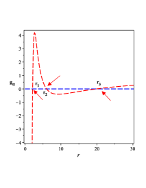
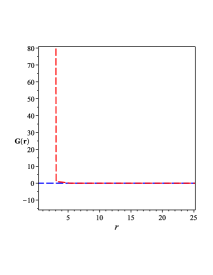
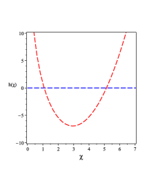
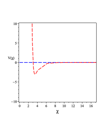
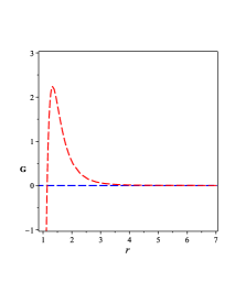
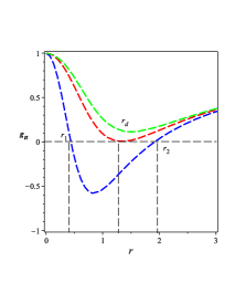
The metric of the line-element (49) has multi-horizons as FIG. 1 0(a) shows. These multi-horizons, three ones, are created due to specific value of the constant $c_{2}$ and other values will create two horizons only. These three multi-horizons are created from the constants $M$ , $c_{1}$ , and $c_{2}$ and the vanishing of the dimensional parameter $c_{2}$ reproduces geometry with two horizons. Moreover, when the dimensional parameters $c_{1}$ and $c_{2}$ vanish, the geometry with one horizon, i.e., the Schwarzschild geometry is reproduced. As Eq. (32) shows, the BH solution (49) gives a non-trivial form of the GB invariant, whose behavior is shown in FIG. 1 0(b). The behavior of the physical quantities, $h(\chi)$ , $V(\chi)$ , and the Lagrange multiplier field $\lambda$ , for the BH solution (III.1) are shown in FIG. 1 0(c), 1 0(d), and 1 0(e).

Refer to caption — (a) The plot of the function $f(r)$ , given by Eq. (III.1), vs. the radial coordinate $r$

Using Eq. (49), we obtain $M$ as a function of the redial coordinate $r$ ,

\displaystyle M=\frac{r}{2}\left(1+\frac{c_{1}}{r^{2}}+\frac{c_{2}}{r^{6}}\right)\,.

(50)

Now we investigate the thermodynamics for the BH (III.1). The Hawking temperature is defined as Sheykhi:2012zz ; Sheykhi:2010zz ; Hendi:2010gq ; Sheykhi:2009pf

\displaystyle T_{2}=\frac{f^{\prime}\left(r_{2}\right)}{4\pi}\,,

(51)

where $r_{2}$ is the event horizon located at $r=r_{2}$ which is the largest positive root of $f\left(r_{2}\right)=0$ which satisfies $f^{\prime}\left(r_{2}\right)\neq 0$ . Using Eq. (51), we obtain the Hawking temperature of the BH solution in the form:

\displaystyle T_{2}=\frac{M{r_{2}}^{5}-c_{1}{r_{2}}^{4}-3c_{2}}{2\pi{r_{2}}^{7}}\,.

(52)

The Hawking entropy is defined as Cognola:2011nj ; Sheykhi:2012zz ; Sheykhi:2010zz ; Hendi:2010gq ; Sheykhi:2009pf ; Zheng:2018fyn

\displaystyle S\left(r_{2}\right)=\frac{1}{4}A\left(r_{2}\right)\,,

(53)

where $A$ is the area of the event horizon.

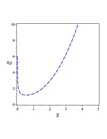
To show how many horizons of the BH solution Eq. (28), we plot $g_{00}$ in FIG. 2 1(a). As FIG. 1 0(a) shows that for specific value of $c_{2}$ , we have three horizons and for other values $c_{2}$ or when $c_{2}=0$ we have two horizons as FIG. 2 1(a). Also in FIG. 2 1(a), we show the region where the black hole has no singularity, i.e., naked singularity.

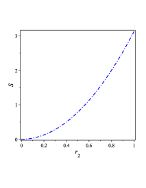
Using Eq. (53), the entropy of the BH (28) is computed as,

\displaystyle S_{2}=\pi{r_{2}}^{2}\,.

(54)

We plot Eq. (54) in FIG. 2 1(b). As this figure show, we have always positive entropy.

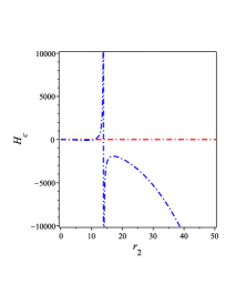
The Hawking temperatures associated with the BH solution (28) is plotted in FIG. 2 1(c). From this figure, one can show that we have always a positive temperature for $r_{2}$ . To investigate the thermodynamical stability of BHs, the formula of the heat capacity $H\left(r_{2}\right)$ at the event horizon should be derived. The heat capacity is defined as follows Nouicer:2007pu ; DK11 ; Chamblin:1999tk ,

\displaystyle H_{c}\equiv H\left(r_{2}\right)=\frac{\partial M_{2}}{\partial T_{2}}=\frac{\partial M_{2}}{\partial r_{2}}\left(\frac{\partial T_{2}}{\partial r_{2}}\right)^{-1}\,.

(55)

The BH will be thermodynamically stable if its heat capacity $H_{c}$ is positive. On the other hand, it will be unstable if $H_{c}$ is negative. As well-known, the heat capacity of the Schwarzschild black hole in GR is negative and therefore the solution is unstabel, which corresponds to the Hawking evaporation. Substituting (50) and (52) into (55), we obtain the heat capacity as follows,

\displaystyle H_{c}=\frac{\pi{r_{2}}^{2}\left(c_{1}{r_{2}}^{4}-{r_{2}}^{6}+5c_{2}\right)}{2M{r_{2}}^{5}-3c_{1}{r_{2}}^{4}-21c_{2}}\,.

(56)

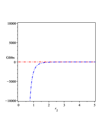
The free energy in the grand canonical ensemble, which is calledthe Gibbs free energy, can be defined as Zheng:2018fyn ; Kim:2012cma ,

\displaystyle G\left(r_{2}\right)=E\left(r_{2}\right)-T\left(r_{2}\right)S\left(r_{2}\right)

(57)

where $E\left(r_{2}\right)$ , $T\left(r_{2}\right)$ , and $S\left(r_{2}\right)$ are the quasi-local energy, the temperature and entropy at the event horizons, respectively. Substituting Eqs. (50), (52), and (53) into (57), we obtain the Gibbs free energy of the BH (28) in the following form,

\displaystyle G\left(r_{2}\right)=\frac{{r_{2}}^{6}+3c_{1}{r_{2}}^{4}+7c_{2}}{4{r_{2}}^{5}}\,.

(58)

We plot the behavior of the Gibbs free energy in FIG. 2 1(e), which shows that the BH solution (28) with $r_{2}$ is unstable.

IV.2 Thermodynamics of the BH (40, III.2)

In this section, we will study the thermodynamics of the BH solution in (40, III.2). For this aim, by assuming $r$ is large, we rewrite the metric as follows,

\displaystyle f(r)=1+\frac{\alpha r^{2}}{r^{3}+\beta}\approx 1-\frac{2M}{r}+\frac{2M\beta}{r^{4}}-\frac{2M\beta^{2}}{r^{7}}\,,\quad\mbox{where}\quad\alpha=-2M\,.

(59)

By using Eqs. (59) and (40) we obtain

\displaystyle ds^{2}=-\left[1-\frac{2M}{r}+\frac{2M\beta}{r^{4}}-\frac{2M\beta^{2}}{r^{7}}\right]dt^{2}+\frac{dr^{2}}{1-\frac{2M}{r}+\frac{\beta}{r^{3}}}+r^{2}\left(d\theta^{2}+\sin^{2}\theta d\phi^{2}\right)\,,

(60)

which is asymptotically approaches flat space-time but is not equal to the Schwarzschild space-time due to the contribution of the extra term including $\beta$ . It is easy to check that when the term $\beta$ vanishes, the geometry reduces to the Schwarzschild space-time. From Eq. (60), we obtain an expression of $M$ in terms of the radial coordinate $r$ as follows,

\displaystyle M=\frac{r}{2}\left(1+\frac{2M\beta}{r^{4}}-\frac{2M\beta^{2}}{r^{7}}\right)\,.

(61)

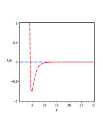
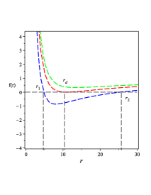
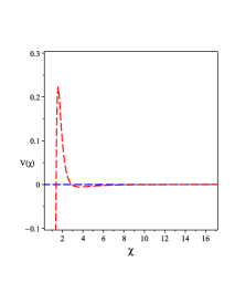
The metric of the line-element given by (60) has two horizons as shown in FIG. 3 2(a) shows. These two horizons are created by the constants $M$ and $\beta$ . When $\beta$ vanishes, the geometry of the Schwarzschild geometry is reproduced. The behavior of the metric is drawn in FIG. 3 2(b), which shows clearly that there are two horizons related to the BH solution (40). As Eq. (48) shows, the BH solution (60) has a non-trivial expression of the GB invriant, whose behavior is shown in FIG. 3 2(c). The behavior of the physical quantities related to the BH solution (III.2) like $h(\chi)$ , $V(\chi)$ , and the Lagrange multiplier field $\lambda$ are shown in FIG. 3 2(d), 3 2(e), and 3 2(f).

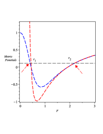
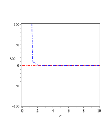
To show how many horizons appear in the BH solution of Eq. (40), we plot the metric $g_{00}$ in FIG. 4 3(a). As FIG. 4 3(b) shows that in the case $\beta=0.3$ ¹¹1In this study we use Eq. (59) and put $\alpha=-2$ which yields $M=1$ ., we have two horizons and when $\beta=1.3$ , we have no horizon. Also in FIG. 4 3(b), we show the region where the black hole has naked singularity, i.e., when $\beta>1.3$ .

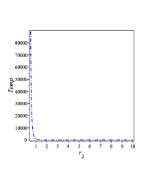
By using Eq. (51), we obtain the Hawking temperature of the BH solution (40) in the following form,

\displaystyle T_{2}=\frac{\alpha r_{2}\left(2\beta-{r_{2}}^{3}\right)}{4\pi\left({r_{2}}^{4}+\beta\right)^{2}}\,,

(62)

We show the behavior of Eq. (62) in FIG. 4 3(b).

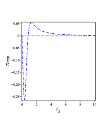
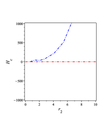
From this figure one can show that we have a positive temperature for $r_{2}>r_{d}$ and negative temperature for $r_{2}<r_{d}$ where $r_{d}$ is the degenerate horizon as shown in FIG. 4 3(a). Substituting (61) and (62) into (55), we obtain the heat capacity as follows,

\displaystyle H_{c}=\frac{2\pi\left(\beta-{r_{2}}^{3}\right)\left({r_{2}}^{3}+\beta\right)}{{r_{2}}^{3}\alpha\left({r_{2}}^{6}-7\beta{r_{2}}^{3}+\beta^{2}\right)}\,.

(63)

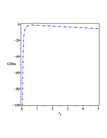
We show the behavior of Eq. (63) in FIG. 4 3(c). By substituting Eqs. (53), (61), and (62) into (58), we obtain the Gibbs free energy of the BH (40) in the following form,

\displaystyle G\left(r_{+}\right)=-\frac{4{r_{2}}^{9}+12\beta{r_{2}}^{6}+12\beta^{2}{r_{2}}^{3}+4\beta^{3}-\alpha{r_{2}}^{8}+2\alpha\beta{r_{2}}^{5}}{4{r_{2}}^{2}({r_{2}}^{3}+\beta)^{2}}\,.

(64)

We plot the behavior of the Gibbs free energy in FIG. 4 3(d), which shows that the BH solution (40) with $r_{2}$ is unstable.

V Motion of Particle

To show the effect of modified GB theory on observables, we study the motion of a test particle in the background solution given by the metric (28) and (40). We consider the photon sphere around the BH and the perihelion shift of circular orbits. For the time being, the photon sphere becomes of particular interest because it explains the edge of the shadow of a BH while the perihelion shift was already derived in Bahamonde:2019zea ; DeBenedictis:2016aze .

V.1 Geodesic equation and effective potential

In this subsection, we study the geodesic equation in the space-time given by Eq. (28). For this aim, we define the worldline $q(\tau)$ of a test particle in a curved space-time by the Euler-Lagrange equations which is defined by,

\displaystyle\frac{d}{d\tau}\left(\frac{\partial\mathcal{L}}{\partial\dot{q}^{\mu}}\right)-\frac{\partial\mathcal{L}}{\partial q^{\mu}}=0\,,

(65)

for the Lagrangian

\displaystyle 2\mathcal{L}=g_{\mu\nu}\dot{q}^{\mu}\dot{q}^{\nu}=f(r)\dot{t}^{2}-\frac{\dot{r}^{2}}{f(r)}-r^{2}\dot{\theta}^{2}-r^{2}\sin^{2}{\theta}\dot{\phi}^{2}\,,

(66)

with $q^{\mu}(\tau)=\left(t\left(\tau\right),r\left(\tau\right),\theta\left(\tau\right),\phi\left(\tau\right)\right)$ and $\dot{q}^{\mu}$ refers to the derivative of $q^{\mu}$ w.r.t. the affine parameter $\tau$ .

We solve the Euler-Lagrange equations (65) in the spherically symmetric space-times and we focus on the motion of the equatorial plane with $\theta=\pi/2$ . under the assumption, we obtain the conserved quantities, i.e., the energy $E$ and angular momentum $L$ as follows,

	$\displaystyle E=$	$\displaystyle\,\frac{\partial\mathcal{L}}{\partial\dot{t}}=f(r)\dot{t}=\left(1-\frac{2M}{r}+\frac{c_{1}}{r^{2}}+\frac{c_{2}}{r^{6}}\right)\dot{t}\,,$		(67)
	$\displaystyle L=$	$\displaystyle\,\frac{\partial\mathcal{L}}{\partial\dot{\phi}}=r^{2}\dot{\phi}\,.$		(68)

Using the above conserved quantities (67) and (68), we obtain the effective potential in classical mechanics. Because $2\mathcal{L}=0$ for the massless particle and $2\mathcal{L}=1$ for the massive particle, by deleting $\dot{t}$ and $\dot{\phi}$ by using Eqs. (67) and (68), and by putting $\theta=\pi/2$ (constant), we obtain

\displaystyle\frac{E^{2}}{1-\frac{2M}{r}+\frac{c_{1}}{r^{2}}+\frac{c_{2}}{r^{6}}}-\frac{\dot{r}^{2}}{1-\frac{2M}{r}+\frac{c_{1}}{r^{2}}+\frac{c_{2}}{r^{6}}}-\frac{L^{2}}{r^{2}}=\sigma\,,

(69)

where $\sigma=0$ for massless particles and $\sigma=1$ . We rewrite Eq. (69) as follows,

\displaystyle 0=\frac{1}{2}\dot{r}^{2}-\frac{1}{2}E^{2}+\frac{1}{2}\frac{L^{2}}{r^{2}}\left(1-\frac{2M}{r}+\frac{c_{1}}{r^{2}}+\frac{c_{2}}{r^{6}}\right)+\frac{1}{2}\sigma\left(1-\frac{2M}{r}+\frac{c_{1}}{r^{2}}+\frac{c_{2}}{r^{6}}\right)\,,

(70)

from which we can read off the effective potential $\mathcal{V}(r)$ ,

\displaystyle\mathcal{V}(r)=

\displaystyle\,\frac{1}{2}\left(1-\frac{2M}{r}+\frac{c_{1}}{r^{2}}+\frac{c_{2}}{r^{6}}\right)\left(\frac{L^{2}}{r^{2}}+\sigma\right)-\frac{1}{2}E^{2}\,,

(71)

and we rewrite (70) as follows,

\displaystyle\frac{1}{2}\dot{r}^{2}+\mathcal{V}(r)=0\,.

(72)

For the study of the perihelion shift, we reparametrize $r(\tau)$ as $r(\phi)$ , which yields,

\displaystyle\frac{1}{2}\frac{\dot{r}^{2}}{\dot{\phi}^{2}}+\frac{1}{\dot{\phi}^{2}}\mathcal{V}(r)=\frac{1}{2}\left(\frac{dr}{d\phi}\right)^{2}+\frac{r^{4}}{L^{2}}\mathcal{V}(r)=0\,.

(73)

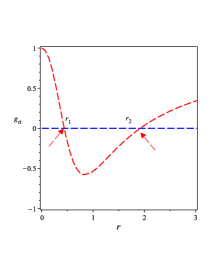
V.2 Photon sphere and perihelion shift of space-time (28)

For a circular orbit where $r=\mbox{const.}$ , $\dot{r}=0$ , the effective potential and its derivative have to vanish i.e., we have to solve both equations $\mathcal{V}=0$ and $\mathcal{V}^{\prime}=0$ .

When $c_{2}=\sigma=0$ , the effective potential $\mathcal{V}(r)$ reduces to,

\displaystyle\mathcal{V}(r)=\frac{1}{2}\left(1-\frac{2M}{r}+\frac{c_{1}}{r^{2}}\right)\frac{L^{2}}{r^{2}}-\frac{1}{2}E^{2}\,.

(74)

When $r$ is large, $\mathcal{V}(r)$ is monotonically decreasing function of $r$ . On the other hand, when $r$ is small, $\mathcal{V}(r)$ behaves as $\mathcal{V}(r)\sim\frac{c_{1}L^{2}}{2r^{4}}$ and therefore if $c_{1}>0$ , $\mathcal{V}(r)$ goes to positive infinity and if $c_{1}<0$ , $\mathcal{V}(r)$ goes to negative infinity.

For circular photon orbits, by solving the equations $\mathcal{V}(r)=\mathcal{V}^{\prime}(r)=0$ for the potential $\mathcal{V}(r)$ in Eq. (74), we find,

	$\displaystyle r=$	$\displaystyle\,\frac{3}{2}M\pm\frac{1}{2}\sqrt{9M^{2}-8c_{1}}\,,$
	$\displaystyle L_{\pm}=$	$\displaystyle\,\pm\frac{(3M+\sqrt{9M^{2}-8c_{1}})^{2}E}{2\sqrt{6M^{2}+2M\sqrt{9M^{2}-8c_{1}}-4c_{1}}}\,,$		(75)

where the value of $r$ given in the first equation of Eq. (V.2) is used in the second equation of (V.2). Eq. (V.2) gives the value of the Schwarzschild when $c_{1}=0$ , i.e., $r=3M$ and $L_{\pm}=3\sqrt{3}M\,E$ .

The expression of $r$ in (V.2) tells that when $c_{1}<0$ , there is only one extremum $r=\frac{3}{2}M+\frac{1}{2}\sqrt{9M^{2}-8c_{1}}$ . The behavior if the potential tells that the extremum is a maximum and therefore the orbit $r$ is unstable. On the other hand, when $\frac{9M^{2}}{8}>c_{1}>0$ , there are two extrema $r=\frac{3}{2}M\pm\frac{1}{2}\sqrt{9M^{2}-8c_{1}}$ . The behavior of the potential tells that the larger extremum $r=\frac{3}{2}M+\frac{1}{2}\sqrt{9M^{2}-8c_{1}}$ is a local maximum and therefore the orbit corresponding to the extremum is unstable but the smaller extremum $r=\frac{3}{2}M-\frac{1}{2}\sqrt{9M^{2}-8c_{1}}$ is a local minimum and therefore the orbit corresponding to the extremum is stable.

For circular timelike orbits $\sigma=1$ for a massive particle, it is also possible to solve the equations $\mathcal{V}=0$ and $\mathcal{V}^{\prime}=0$ . The obtained expressions are, however, not so insightful. We consider a perturbation around a circular orbit $r=r_{\mathrm{crc.}}$ and by plugging in the ansatz $r(\phi)=r_{\mathrm{crc.}}+r_{\phi}(\phi)$ for (73), we obtain,

\displaystyle\left(\frac{dr_{\phi}}{d\phi}\right)^{2}=-2\frac{(r_{\mathrm{crc.}}+r_{\phi})^{4}}{h^{2}}\mathcal{V}\left(r_{\mathrm{crc.}}+r_{\phi}\right)\,.

(76)

Assuming that the ratio $r_{\phi}/r_{c}$ is small, the right-hand side can be expanded into powers of this parameter to second order

\displaystyle\left(\frac{dr_{\phi}}{d\phi}\right)^{2}=-\frac{r_{\mathrm{crc.}}^{4}}{h^{2}}\mathcal{V}^{\prime\prime}\left(r_{\mathrm{crc.}}\right){r_{\phi}}^{2}+\mathcal{O}\left(\tfrac{{r_{\phi}}^{3}}{{r_{\mathrm{crc.}}}^{3}}\right)\,,

(77)

where we use the fact that $V\left(r_{\mathrm{crc.}}\right)=0$ and $V^{\prime}\left(r_{\mathrm{crc.}}\right)=0$ for circular orbits, as discussed above. The above equation, which represents a simple harmonic oscillation, shows that the solution of $r_{\phi}$ oscillates with a wave number $K=\sqrt{\frac{r_{c}^{4}}{h^{2}}\mathcal{V}^{\prime\prime}\left(r_{\mathrm{crc.}}\right)}$ and thus the perihelion shift is given as,

\displaystyle\Delta\phi=2\pi\left(\frac{1}{K}-1\right)=2\pi\left(\frac{h}{{r_{\mathrm{crc.}}}^{2}\sqrt{\mathcal{V}^{\prime\prime}\left(r_{\mathrm{crc.}}\right)}}-1\right)\,.

(78)

Now, we derive the explicit form of the perihelion shift for massive objects where the potential $\mathcal{V}$ with $\sigma=1$ . We evaluate the equations $\mathcal{V}\left(r_{\mathrm{crc.}}\right)=0$ and $\mathcal{V}^{\prime}\left(r_{\mathrm{crc.}}\right)=0$ with $L=L_{0}+\epsilon\,L_{1}$ and $E=E_{0}+\epsilon\,E_{1}$ . The zeroth order behaviors of these equations determine $L_{0}\left(r_{\mathrm{crc.}}\right)$ and $E_{0}\left(r_{\mathrm{crc.}}\right)$ as follows,

	$\displaystyle L_{0\pm}=$	$\displaystyle\,\pm{\frac{\sqrt{M{r_{\mathrm{crc.}}}^{5}-c_{1}r^{4}-3c_{2}}r}{\sqrt{{r_{\mathrm{crc.}}}^{6}-3M{r_{\mathrm{crc.}}}^{5}+2c_{1}{r_{\mathrm{crc.}}}^{4}+4c_{2}}}}\,,$
	$\displaystyle E_{0\pm}=$	$\displaystyle\,\pm{\frac{\sqrt{4M^{2}{r_{\mathrm{crc.}}}^{5}-2c_{1}{r_{\mathrm{crc.}}}^{4}M-4{r_{\mathrm{crc.}}}^{6}M+{r_{\mathrm{crc.}}}^{7}+c_{2}r_{\mathrm{crc.}}+c_{1}{r_{\mathrm{crc.}}}^{5}-2c_{2}M}}{\sqrt{r_{\mathrm{crc.}}-3\,M}{r_{\mathrm{crc.}}}^{3}}}\,.$		(79)

Having obtained the constants of motion for the circular orbit, we derive the perihelion shift by plugging in the values into $\mathcal{V}^{\prime\prime}(r_{\mathrm{crc.}},L_{0},E_{0})$ to obtain $\mathcal{V}^{\prime\prime}\left(r_{\mathrm{crc.}}\right)$ alone. Due to the different solutions for the constants of motion, there exist two options to derive the perihelion shift

\displaystyle\Delta\phi\left(L_{0+}\right)\,,\quad\Delta\phi\left(L_{0-}\right)\,,

(80)

which are related to each other through

\displaystyle\Delta\phi\left(L_{0-}\right)=-4\pi-\Delta\phi\left(L_{0+}\right)\,.

(81)

By expanding the perihelion shift into a power series in the variables $q=\frac{M}{r_{\mathrm{crc.}}}$ , $q_{1}=\frac{c_{1}}{{r_{\mathrm{crc.}}}^{2}}$ , and $q_{2}=\frac{c_{2}}{{r_{\mathrm{crc.}}}^{6}}$ , we obtain

$\displaystyle\Delta\phi\left(L_{0-}\right)=$	$\displaystyle\,12\left({\frac{\pi\left(\sqrt{q-q_{1}-3q_{2}}+\sqrt{q+12\,q_{2}}\right)}{\left(q+12q_{2}\right)^{5/2}}}-{\frac{\pi}{\left(q+12q_{2}\right)^{2}}}\right){q_{1}}^{4}$
	$\displaystyle\,+\left\{\frac{18\pi\left(\sqrt{q-q_{1}-3q_{2}}+\sqrt{(q+12q_{2})}\right)\left(4q_{2}-3q\right)}{\left(q+12q_{2}\right)^{5/2}}-{\frac{3\pi\left(72q-96q_{2}\right)}{4\left(q+12q_{2}\right)^{2}}}\right\}{q_{1}}^{3}$
	$\displaystyle\,-\pi\left(\frac{4}{q+12q_{2}}+{\frac{4\left(\sqrt{q-q_{1}-3q_{2}}+\sqrt{q+12q_{2}}\right)}{\left(q+12q_{2}\right)^{3/2}}}+{\frac{3}{4\left(q+12q_{2}\right)^{2}}}\left(8\left[24{q_{2}}^{2}-qq_{2}+6q^{2}\right]+3\left(4q_{2}-3q\right)^{2}\right)\right.$
	$\displaystyle\,\left.+{\frac{3\pi\left(\sqrt{q-q_{1}-3q_{2}}+\sqrt{q+12q_{2}}\right)\left(192{q_{2}}^{2}-8qq_{2}+48q^{2}+\left(12q_{2}-9q\right)^{2}\right)}{4\left(q+12q_{2}\right)^{5/2}}}\right){q_{1}}^{2}$
	$\displaystyle+\left({\frac{\pi\left(12q_{2}-9q\right)}{-q-12q_{2}}}-{\frac{3\pi\left(\sqrt{q-q_{1}-3q_{2}}+\sqrt{q+12q_{2}}\right)\left(4q_{2}-3q\right)}{\left(q+12q_{2}\right)^{3/2}}}-{\frac{9\pi\left(24{q_{2}}^{2}-qq_{2}+6q^{2}\right)\left(4q_{2}-3q\right)}{2\left(-q-12q_{2}\right)^{2}}}\right.$
	$\displaystyle\left.+{\frac{3\pi\left(\sqrt{q-q_{1}-3q_{2}}+\sqrt{q+12q_{2}}\right)\left(24{q_{2}}^{2}-qq_{2}+6q^{2}\right)\left(12q_{2}-9q\right)}{2\left(q+12q_{2}\right)^{5/2}}}\right)q_{1}$
	$\displaystyle\,+2{\frac{2\pi\left(\sqrt{q-q_{1}-3q_{2}}+\sqrt{q+12q_{2}}\right)}{\sqrt{q+12q_{2}}}}+{\frac{3\pi\left(\sqrt{q-q_{1}-3q_{2}}+\sqrt{q+12q_{2}}\right)\left(24{q_{2}}^{2}-qq_{2}+6q^{2}\right)^{2}}{4\left(q+12q_{2}\right)^{5/2}}}$
	$\displaystyle\,-{\frac{3\pi\left(24{q_{2}}^{2}-qq_{2}+6q^{2}\right)^{2}}{4\left(-q-12q_{2}\right)^{2}}}-{\frac{\pi\left(\sqrt{q-q_{1}-3q_{2}}+\sqrt{q+12q_{2}}\right)\left(24{q_{2}}^{2}-qq_{2}+6q^{2}\right)}{\left(q+12q_{2}\right)^{3/2}}}$
	$\displaystyle\,-{\frac{\pi\left(24{q_{2}}^{2}-qq_{2}+6q^{2}\right)}{q+12\,q_{2}}}+\mathcal{O}\left(\left(qq_{1}q_{2}\right)^{3}\right)\,.$	(82)

Eq. (V.2) when $q_{1}=q_{2}=0$ , i.e., $c_{1}=c_{2}=0$ , yields

\displaystyle\Delta\phi\left(L_{0-}\right)=6\pi q+27\pi q^{2}+\mathcal{O}\left(q^{3}\right)\,,

(83)

which coincides with the perihelion of the Schwarzschild solution.

The qualitative behavior of the perihelion shift is always the same, only the numerical values differ. Eq. (V.2) shows that $q>q_{1}+3q_{2}$ , and the higher $q_{1}$ and $q_{2}$ , the smaller the influence of the perturbation and corrections to the perihelion shift appear only in higher orders in $q$ .

Now we repeat the above perihelion of the BH solution (28) to the BH (40).

V.3 Photon sphere and perihelion shift in space-time (40)

For the Lagrangian

\displaystyle 2\mathcal{L}=g_{\mu\nu}\dot{q}^{\mu}\dot{q}^{\nu}=f(r)\dot{t}^{2}-\frac{\dot{r}^{2}}{f_{1}(r)}-r^{2}\dot{\theta}^{2}-r^{2}\sin^{2}{\theta}\dot{\phi}^{2}\,,

(84)

with $q^{\mu}(\tau)=\left(t\left(\tau\right),r\left(\tau\right),\theta\left(\tau\right),\phi\left(\tau\right)\right)$ , and $\dot{q}^{\mu}$ refers to the derivative of $q^{\mu}$ w.r.t. the affine parameter $\tau$ .

To solve the Euler-Lagrange equations, we apply the same procedure used above for the BH (28). For the BH solution (40), we obtain the energy $E$ and angular momentum $L$ as follows,

	$\displaystyle E=$	$\displaystyle\,\frac{\partial\mathcal{L}}{\partial\dot{t}}=f(r)\dot{t}=\left(1+\frac{\alpha r^{2}}{r^{3}+\beta}\right)\dot{t}\,,$		(85)
	$\displaystyle L=$	$\displaystyle\,\frac{\partial\mathcal{L}}{\partial\dot{\phi}}=r^{2}\dot{\phi}\,.$		(86)

Using the above expressions, we obtain the effective potential by rewriting the Lagrangian (84),

\displaystyle\frac{E^{2}}{1+\frac{\alpha r^{2}}{r^{3}+\beta}}-\frac{\dot{r}^{2}}{1+\frac{\alpha}{r}+\frac{\beta}{r^{3}}}-\frac{L^{2}}{r^{2}}=\sigma\,.

(87)

The corresponding effective potential of the BH solution (40) takes the following form,

\displaystyle\mathcal{V}(r)

\displaystyle=\frac{L^{2}}{2r^{2}}\left(1+\frac{\alpha}{r}+\frac{\beta}{r^{3}}\right)+\frac{\sigma}{2}\left(1+\frac{\alpha}{r}+\frac{\beta}{r^{3}}\right)-\frac{E^{2}\left(1+\frac{\alpha}{r}+\frac{\beta}{r^{3}}\right)}{2\left(1+\frac{\alpha r^{2}}{r^{3}+\beta}\right)}\,.

(88)

For circular photon orbits, $\sigma=0$ , solving the zeroth order equations yields,

\displaystyle 0=-2{r_{0}}^{3}{L_{0}}^{2}+3{r_{0}}^{2}\beta{E_{0}}^{2}+6{r_{0}}^{2}M{L_{0}}^{2}-5\beta{L_{0}}^{2}\,,\quad L_{0\pm}=\pm E_{0}r_{0}\sqrt{\frac{{r_{0}}^{3}+\beta}{{{r_{0}}^{3}+\beta-2M{r_{0}}^{2}}}}\,.

(89)

Eq. (89) shows that when the dimensional constant $\beta$ vanishes, we obtain the zeroth order terms of $r_{0}$ and $L_{0}$ of the Schwarzschild space-time when $\sigma=0$ , i.e., $r_{0}=3M$ and $L_{0\pm}=\pm 3\sqrt{3}ME_{0}$ . The above equation has three roots for $r_{0}$ , one of them has a real value and takes the following form,

	$\displaystyle r_{0}=$	$\displaystyle\,\frac{\sqrt[3]{\beta^{3}{E_{0}}^{6}-10\beta{L_{0}}^{6}+6\beta^{2}{E_{0}}^{4}{L_{0}}^{2}M+12\beta{E_{0}}^{2}{L_{0}}^{4}M^{2}-8{L_{0}}^{6}M^{3}-16S{L_{0}}^{3}}}{2{L_{0}}^{2}}$
		$\displaystyle\,+\frac{\left(\beta{E_{0}}^{2}+2{L_{0}}^{2}M\right)^{2}}{2{L_{0}}^{2}\sqrt[3]{\beta^{3}{E_{0}}^{6}-10\beta{L_{0}}^{6}+6\beta^{2}{E_{0}}^{4}{L_{0}}^{2}M+12\beta{E_{0}}^{2}{L_{0}}^{4}M^{2}-8{L_{0}}^{6}M^{3}-16S{L_{0}}^{3}}}+\frac{\beta\,{E_{0}}^{2}+{2ML_{0}}^{2}}{2{L_{0}}^{2}}\,,$		(90)

where $S=\sqrt{5\beta\left({L_{0}}^{6}M^{3}+5\beta{L_{0}}^{6}-\beta^{3}{E_{0}}^{6}-6\beta^{2}{E_{0}}^{4}{L_{0}}^{2}M+12\beta{E_{0}}^{2}{L_{0}}^{4}M^{2}\right)}$ . The above equation gives the value of the Schwarzschild space-time when $\beta=0$ .

Now we derive the explicit form of the perihelion shift for massive particles for the BH (40) by using the potential $\mathcal{V}$ (88) with $\sigma=1$ . We evaluate the equations $\mathcal{V}(r_{c}rc.)=0$ and $\mathcal{V}^{\prime}\left(r_{\mathrm{crc.}}\right)=0$ by considering the perturbation with $L=L_{0}+\epsilon h_{1}$ and $k=k_{0}+\epsilon k_{1}$ . The zeroth order terms of these equations determine $L_{0}\left(r_{\mathrm{crc.}}\right)$ and $E_{0}\left(r_{\mathrm{crc.}}\right)$ as follows,

\displaystyle E_{0\pm}=\pm\frac{\sqrt{2}({r_{\mathrm{crc.}}}^{3}-2M{r_{\mathrm{crc.}}}^{3}+\beta)}{\sqrt{2{r_{\mathrm{crc.}}}^{6}-6M{r_{\mathrm{crc.}}}^{5}+4\beta{r_{\mathrm{crc.}}}^{3}+2\beta^{2}}}\,,\quad L_{0\pm}=\pm{r_{\mathrm{crc.}}}^{2}\sqrt{\frac{2M{r_{\mathrm{crc.}}}^{3}+4M\beta}{2r^{6}-6M{r_{\mathrm{crc.}}}^{5}+4\beta{r_{\mathrm{crc.}}}^{3}+2\beta^{2}}}\,.

(91)

By using the obtained constants of motion for the circular orbit, we derive the perihelion shift by plugging of the expressios of $E_{0}=E_{0\pm}$ , $L_{0}=L_{0\pm}$ into $V^{\prime\prime}\left(r_{\mathrm{crc.}},E_{0},L_{0}\right)$ . Corresponding to the signatures $\pm$ in the expressions of $E_{0}=E_{0\pm}$ and $L_{0}=L_{0\pm}$ , there exist two options to derive the perihelion shift,

\displaystyle\Delta\phi\left(L_{0+}\right)\,,\quad\Delta\phi\left(L_{0-}\right)\,,

(92)

which are related to each other through

\displaystyle\Delta\phi\left(L_{0-}\right)

\displaystyle=-4\pi-\Delta\phi\left(L_{0+}\right)\,.

(93)

By expanding the perihelion shift into a power series of $q=\frac{M}{r_{\mathrm{crc.}}}$ and $q_{1}=\frac{\beta}{{r_{\mathrm{crc.}}}^{3}}$ , we obtain

\displaystyle\Delta\phi\left(L_{0-}\right)=2\frac{\sqrt{1-2q_{1}}-\sqrt{1-6q+11q_{1}-8q_{1}{}^{2}}}{\sqrt{1-6q+11q_{1}-8q_{1}{}^{2}}}\,.

(94)

Eq. (94) when $q_{1}=0$ yields,

\displaystyle\Delta\phi\left(L_{0-}\right)\approx 6\pi q+27\pi q^{2}-13\pi q_{1}-105\pi qq_{1}+\frac{435\pi}{4}q_{1}{}^{2}+\mathcal{O}\left(\left(qq_{1}\right)^{3}\right)\,,

(95)

which coincides with the perihelion shift of the Schwarzschild solution when $q_{1}=0$ .

The qualitative behavior of the perihelion shift is not so changed, only the numerical values differ. As for the photon sphere, the higher $q_{1}$ , the higher the influence of the perturbation and corrections to the perihelion shift appear.

VI Conclusions

In this study, we constructed a consistent ghost-free modified GB gravitational theory capable of describing BH with horizons. The field equations of this theory are applied to a spherically symmetric space-time and we succeeded to derive BH solutions with multi-horizons. We showed that for the Schwarzschild BH type metric (21), we obtained a BH solution with three horizons and the curvature invariants of this BH show a true singularity at $r=0$ . Moreover, we calculated the thermodynamical quantities associated with this solution and showed that all the thermodynamical quantities and the heat capacity and Gibbs free energy tell that this solution is not stable.

We repeated our calculations for a more general case whose metric is given by (33) and showed that the solution has two horizons in spite that the field equations do not include cosmological constant nor there is not any source of charge to reproduce such two horizons. Moreover, we also showed that such BH yields a true singularity at $r=0$ . We also calculated the thermodynamical quantities and showed that the Gibbs is negative. Furthermore, for both BH solutions in (21) and (33), we calculated all the physical quantities which appear in the GFGB theory, that is, the potential, the Lagrange multiplier, and the function $f$ and showed their behaviors in FIG. 1 and 3.

We should note that the present study is a first trial in the direction of a full phenomenological classification of observables, which is derived in the weak GFGB gravity, to compare them with observations. The future work in this direction could be to study axially symmetric perturbations around rotating space-time, to obtain the shift in the photon regions, that will give an important imprint on the predictions of the shape of the BH shadow. This case will be studied elsewhere.

References

(1) C. M. Will, Living Rev. Rel. 17 (2014), 4 doi:10.12942/lrr-2014-4 [arXiv:1403.7377 [gr-qc]].
(2) M. Ishak, Living Rev. Rel. 22 (2019) no.1, 1 doi:10.1007/s41114-018-0017-4 [arXiv:1806.10122 [astro-ph.CO]].
(3) D. Lovelock, J. Math. Phys. 12 (1971), 498-501 doi:10.1063/1.1665613
(4) T. Clifton, P. G. Ferreira, A. Padilla and C. Skordis, Phys. Rept. 513 (2012), 1-189 doi:10.1016/j.physrep.2012.01.001 [arXiv:1106.2476 [astro-ph.CO]].
(5) T. Padmanabhan and D. Kothawala, Phys. Rept. 531 (2013), 115-171 doi:10.1016/j.physrep.2013.05.007 [arXiv:1302.2151 [gr-qc]].
(6) S.-shen Chern, Annals of Mathematics 46 (1945), 674.
(7) S. Ferrara, R. R. Khuri and R. Minasian, Phys. Lett. B 375 (1996), 81-88 doi:10.1016/0370-2693(96)00270-5 [arXiv:hep-th/9602102 [hep-th]].
(8) I. Antoniadis, S. Ferrara, R. Minasian and K. S. Narain, Nucl. Phys. B 507 (1997), 571-588 doi:10.1016/S0550-3213(97)00572-5 [arXiv:hep-th/9707013 [hep-th]].
(9) B. Zwiebach, Phys. Lett. B 156 (1985), 315-317 doi:10.1016/0370-2693(85)91616-8
(10) R. I. Nepomechie, Phys. Rev. D 32 (1985), 3201 doi:10.1103/Nepomechie:1985us
(11) C. G. Callan, Jr., I. R. Klebanov and M. J. Perry, Nucl. Phys. B 278 (1986), 78-90 doi:10.1016/0550-3213(86)90107-0
(12) P. Candelas, G. T. Horowitz, A. Strominger and E. Witten, Nucl. Phys. B 258 (1985), 46-74 doi:10.1016/0550-3213(85)90602-9
(13) D. J. Gross and J. H. Sloan, Nucl. Phys. B 291 (1987), 41-89 doi:10.1016/0550-3213(87)90465-2
(14) D. Glavan and C. Lin, Phys. Rev. Lett. 124 (2020) no.8, 081301 doi:10.1103/Glavan:2019inb [arXiv:1905.03601 [gr-qc]].
(15) A. Kumar, R. K. Walia and S. G. Ghosh, Universe 8 (2022) no.4, 232 doi:10.3390/universe8040232 [arXiv:2003.13104 [gr-qc]].
(16) P. G. S. Fernandes, Phys. Lett. B 805 (2020), 135468 doi:10.1016/j.physletb.2020.135468 [arXiv:2003.05491 [gr-qc]].
(17) R. Kumar and S. G. Ghosh, JCAP 07 (2020), 053 doi:10.1088/1475-7516/2020/07/053 [arXiv:2003.08927 [gr-qc]].
(18) S. G. Ghosh and R. Kumar, Class. Quant. Grav. 37 (2020) no.24, 245008 doi:10.1088/1361-6382/abc134 [arXiv:2003.12291 [gr-qc]].
(19) S. L. Li, P. Wu and H. Yu, [arXiv:2004.02080 [gr-qc]].
(20) T. Kobayashi, JCAP 07 (2020), 013 doi:10.1088/1475-7516/2020/07/013 [arXiv:2003.12771 [gr-qc]].
(21) S. G. Ghosh and S. D. Maharaj, Phys. Dark Univ. 30 (2020), 100687 doi:10.1016/j.dark.2020.100687 [arXiv:2003.09841 [gr-qc]].
(22) T. Shirafuji, G. G. L. Nashed and Y. Kobayashi, Prog. Theor. Phys. 96, 933-948 (1996) doi:10.1143/PTP.96.933 [arXiv:gr-qc/9609060 [gr-qc]].
(23) D. Malafarina, B. Toshmatov and N. Dadhich, Phys. Dark Univ. 30 (2020), 100598 doi:10.1016/j.dark.2020.100598 [arXiv:2004.07089 [gr-qc]].
(24) D. D. Doneva and S. S. Yazadjiev, JCAP 05 (2021), 024 doi:10.1088/1475-7516/2021/05/024 [arXiv:2003.10284 [gr-qc]].
(25) R. A. Konoplya and A. Zhidenko, Phys. Rev. D 101 (2020) no.8, 084038 doi:10.1103/PhysRevD.101.084038 [arXiv:2003.07788 [gr-qc]].
(26) B. Eslam Panah, K. Jafarzade and S. H. Hendi, Nucl. Phys. B 961 (2020), 115269 doi:10.1016/j.nuclphysb.2020.115269 [arXiv:2004.04058 [hep-th]].
(27) S. A. Hosseini Mansoori, Phys. Dark Univ. 31 (2021), 100776 doi:10.1016/j.dark.2021.100776 [arXiv:2003.13382 [gr-qc]].
(28) R. A. Konoplya and A. F. Zinhailo, Phys. Lett. B 810 (2020), 135793 doi:10.1016/j.physletb.2020.135793 [arXiv:2004.02248 [gr-qc]].
(29) K. Hegde, A. Naveena Kumara, C. L. A. Rizwan, A. K. M. and M. S. Ali, [arXiv:2003.08778 [gr-qc]].
(30) M. Guo and P. C. Li, Eur. Phys. J. C 80 (2020) no.6, 588 doi:10.1140/epjc/s10052-020-8164-7 [arXiv:2003.02523 [gr-qc]].
(31) Y. P. Zhang, S. W. Wei and Y. X. Liu, Universe 6 (2020) no.8, 103 doi:10.3390/universe6080103 [arXiv:2003.10960 [gr-qc]].
(32) R. Roy and S. Chakrabarti, Phys. Rev. D 102 (2020) no.2, 024059 doi:10.1103/PhysRevD.102.024059 [arXiv:2003.14107 [gr-qc]].
(33) A. Naveena Kumara, C. L. A. Rizwan, K. Hegde, M. S. Ali and K. M. Ajith, Annals Phys. 434 (2021), 168599 doi:10.1016/j.aop.2021.168599 [arXiv:2004.04521 [gr-qc]].
(34) C. Liu, T. Zhu and Q. Wu, Chin. Phys. C 45 (2021) no.1, 015105 doi:10.1088/1674-1137/abc16c [arXiv:2004.01662 [gr-qc]].
(35) M. Heydari-Fard, M. Heydari-Fard and H. R. Sepangi, Eur. Phys. J. C 81 (2021) no.5, 473 doi:10.1140/epjc/s10052-021-09266-7 [arXiv:2105.09192 [gr-qc]].
(36) R. Kumar, S. U. Islam and S. G. Ghosh, Eur. Phys. J. C 80 (2020) no.12, 1128 doi:10.1140/epjc/s10052-020-08606-3 [arXiv:2004.12970 [gr-qc]].
(37) G. G. L. Nashed, Int. J. Mod. Phys. D 27, no.7, 1850074 (2018) doi:10.1142/S0218271818500748
(38) S. U. Islam, R. Kumar and S. G. Ghosh, JCAP 09 (2020), 030 doi:10.1088/1475-7516/2020/09/030 [arXiv:2004.01038 [gr-qc]].
(39) A. K. Mishra, Gen. Rel. Grav. 52 (2020) no.11, 106 doi:10.1007/s10714-020-02763-2 [arXiv:2004.01243 [gr-qc]].
(40) S. Devi, R. Roy and S. Chakrabarti, Eur. Phys. J. C 80 (2020) no.8, 760 doi:10.1140/epjc/s10052-020-8311-1 [arXiv:2004.14935 [gr-qc]].
(41) M. S. Churilova, Annals Phys. 427 (2021), 168425 doi:10.1016/j.aop.2021.168425 [arXiv:2004.14172 [gr-qc]].
(42) M. Gürses, T. Ç. Şişman and B. Tekin, Eur. Phys. J. C 80 (2020) no.7, 647 doi:10.1140/epjc/s10052-020-8200-7 [arXiv:2004.03390 [gr-qc]].
(43) M. Gurses, T. Ç. Şişman and B. Tekin, Phys. Rev. Lett. 125 (2020) no.14, 149001 doi:10.1103/PhysRevLett.125.149001 [arXiv:2009.13508 [gr-qc]].
(44) J. Arrechea, A. Delhom and A. Jiménez-Cano, Chin. Phys. C 45 (2021) no.1, 013107 doi:10.1088/1674-1137/abc1d4 [arXiv:2004.12998 [gr-qc]].
(45) G. G. L. Nashed, Eur. Phys. J. C 49, 851-857 (2007) doi:10.1140/epjc/s10052-006-0154-x [arXiv:0706.0260 [gr-qc]].
(46) J. Arrechea, A. Delhom and A. Jiménez-Cano, Phys. Rev. Lett. 125 (2020) no.14, 149002 doi:10.1103/PhysRevLett.125.149002 [arXiv:2009.10715 [gr-qc]].
(47) J. Bonifacio, K. Hinterbichler and L. A. Johnson, Phys. Rev. D 102 (2020) no.2, 024029 doi:10.1103/PhysRevD.102.024029 [arXiv:2004.10716 [hep-th]].
(48) G. G. L. Nashed and E. N. Saridakis, Class. Quant. Grav. 36, no.13, 135005 (2019) doi:10.1088/1361-6382/ab23d9 [arXiv:1811.03658 [gr-qc]].
(49) W. Y. Ai, Commun. Theor. Phys. 72 (2020) no.9, 095402 doi:10.1088/1572-9494/aba242 [arXiv:2004.02858 [gr-qc]].
(50) S. Mahapatra, Eur. Phys. J. C 80 (2020) no.10, 992 doi:10.1140/epjc/s10052-020-08568-6 [arXiv:2004.09214 [gr-qc]].
(51) G. G. L. Nashed, Astrophys. Space Sci. 330, 173 (2010) doi:10.1007/s10509-010-0375-1 [arXiv:1503.01379 [gr-qc]].
(52) M. Hohmann, C. Pfeifer and N. Voicu, Eur. Phys. J. Plus 136 (2021) no.2, 180 doi:10.1140/epjp/s13360-021-01153-0 [arXiv:2009.05459 [gr-qc]].
(53) L. M. Cao and L. B. Wu, Eur. Phys. J. C 82 (2022) no.2, 124 doi:10.1140/epjc/s10052-022-10079-5 [arXiv:2103.09612 [gr-qc]].
(54) H. Lu and Y. Pang, Phys. Lett. B 809 (2020), 135717 doi:10.1016/j.physletb.2020.135717 [arXiv:2003.11552 [gr-qc]].
(55) P. G. S. Fernandes, P. Carrilho, T. Clifton and D. J. Mulryne, Phys. Rev. D 102 (2020) no.2, 024025 doi:10.1103/PhysRevD.102.024025 [arXiv:2004.08362 [gr-qc]].
(56) R. A. Hennigar, D. Kubizňák, R. B. Mann and C. Pollack, JHEP 07 (2020), 027 doi:10.1007/JHEP07(2020)027 [arXiv:2004.09472 [gr-qc]].
(57) K. Aoki, M. A. Gorji and S. Mukohyama, Phys. Lett. B 810 (2020), 135843 doi:10.1016/j.physletb.2020.135843 [arXiv:2005.03859 [gr-qc]].
(58) P. G. S. Fernandes, Phys. Rev. D 103 (2021) no.10, 104065 doi:10.1103/PhysRevD.103.104065 [arXiv:2105.04687 [gr-qc]].
(59) Z. C. Lin, K. Yang, S. W. Wei, Y. Q. Wang and Y. X. Liu, Eur. Phys. J. C 80 (2020) no.11, 1033 doi:10.1140/epjc/s10052-020-08612-5 [arXiv:2006.07913 [gr-qc]].
(60) T. Takahashi and J. Soda, Prog. Theor. Phys. 124 (2010), 711-729 doi:10.1143/PTP.124.711 [arXiv:1008.1618 [gr-qc]].
(61) T. Takahashi and J. Soda, Prog. Theor. Phys. 124 (2010), 911-924 doi:10.1143/PTP.124.911 [arXiv:1008.1385 [gr-qc]].
(62) R. A. Konoplya and A. F. Zinhailo, Eur. Phys. J. C 80 (2020) no.11, 1049 doi:10.1140/epjc/s10052-020-08639-8 [arXiv:2003.01188 [gr-qc]].
(63) R. A. Konoplya and A. Zhidenko, Phys. Dark Univ. 30 (2020), 100697 doi:10.1016/j.dark.2020.100697 [arXiv:2003.12492 [gr-qc]].
(64) H. S. Vieira, [arXiv:2107.02065 [gr-qc]].
(65) R. P. Woodard, Scholarpedia 10 (2015) no.8, 32243 doi:10.4249/scholarpedia.32243 [arXiv:1506.02210 [hep-th]].
(66) A. De Felice and T. Suyama, JCAP 06 (2009), 034 doi:10.1088/1475-7516/2009/06/034 [arXiv:0904.2092 [astro-ph.CO]].
(67) S. Nojiri, S. D. Odintsov and V. K. Oikonomou, Phys. Rev. D 99 (2019) no.4, 044050 doi:10.1103/PhysRevD.99.044050 [arXiv:1811.07790 [gr-qc]].
(68) S. Nojiri, S. D. Odintsov, V. K. Oikonomou and A. A. Popov, Nucl. Phys. B 973 (2021), 115617 doi:10.1016/j.nuclphysb.2021.115617 [arXiv:2111.09457 [gr-qc]].
(69) S. Nojiri, S. D. Odintsov and M. Sasaki, Phys. Rev. D 71 (2005), 123509 doi:10.1103/PhysRevD.71.123509 [arXiv:hep-th/0504052 [hep-th]].
(70) A. H. Chamseddine and V. Mukhanov, JHEP 11 (2013), 135 doi:10.1007/JHEP11(2013)135 [arXiv:1308.5410 [astro-ph.CO]].
(71) S. Nojiri and S. D. Odintsov, [erratum: Mod. Phys. Lett. A 29 (2014) no.40, 1450211] doi:10.1142/S0217732314502113 [arXiv:1408.3561 [hep-th]].
(72) J. Dutta, W. Khyllep, E. N. Saridakis, N. Tamanini and S. Vagnozzi, JCAP 02 (2018), 041 doi:10.1088/1475-7516/2018/02/041 [arXiv:1711.07290 [gr-qc]].
(73) S. Nojiri and G. G. L. Nashed, Phys. Lett. B 830 (2022), 137140 doi:10.1016/j.physletb.2022.137140 [arXiv:2202.03693 [gr-qc]].
(74) G. L. L. Nashed and S. Nojiri, JCAP 11 (2021) no.11, 007 doi:10.1088/1475-7516/2021/11/007 [arXiv:2109.02638 [gr-qc]].
(75) A. Sheykhi, Phys. Rev. D 86 (2012), 024013 doi:10.1103/Sheykhi:2012zz [arXiv:1209.2960 [hep-th]].
(76) A. Sheykhi, Eur. Phys. J. C 69 (2010), 265-269 doi:10.1140/epjc/s10052-010-1372-9 [arXiv:1012.0383 [hep-th]].
(77) S. H. Hendi, A. Sheykhi and M. H. Dehghani, Eur. Phys. J. C 70 (2010), 703-712 doi:10.1140/epjc/s10052-010-1483-3 [arXiv:1002.0202 [hep-th]].
(78) A. Sheykhi, M. H. Dehghani and S. H. Hendi, Phys. Rev. D 81 (2010), 084040 doi:10.1103/Sheykhi:2009pf [arXiv:0912.4199 [hep-th]].
(79) G. Cognola, O. Gorbunova, L. Sebastiani and S. Zerbini, Phys. Rev. D 84 (2011), 023515 doi:10.1103/Cognola:2011nj [arXiv:1104.2814 [gr-qc]].
(80) Y. Zheng and R. J. Yang, Eur. Phys. J. C 78 (2018) no.8, 682 doi:10.1140/epjc/s10052-018-6167-4 [arXiv:1806.09858 [gr-qc]].
(81) K. Nouicer, Class. Quant. Grav. 24 (2007), 5917-5934 [erratum: Class. Quant. Grav. 24 (2007), 6435] doi:10.1088/0264-9381/24/24/C02 [arXiv:0706.2749 [gr-qc]].
(82) I. Dymnikova and M. Korpusik, Entropy 13 (2011), 1967 doi:10.3390/e13121967
(83) A. Chamblin, R. Emparan, C. V. Johnson and R. C. Myers, Phys. Rev. D 60 (1999), 064018 doi:10.1103/PhysRevD.60.064018 [arXiv:hep-th/9902170 [hep-th]].
(84) W. Kim and Y. Kim, Phys. Lett. B 718 (2012), 687-691 doi:10.1016/j.physletb.2012.11.017 [arXiv:1207.5318 [gr-qc]].
(85) S. Bahamonde, K. Flathmann and C. Pfeifer, Phys. Rev. D 100 (2019) no.8, 084064 doi:10.1103/PhysRevD.100.084064 [arXiv:1907.10858 [gr-qc]].
(86) A. DeBenedictis and S. Ilijic, Phys. Rev. D 94 (2016) no.12, 124025 doi:10.1103/PhysRevD.94.124025 [arXiv:1609.07465 [gr-qc]].

Multi-horizons black hole solutions, photon sphere and perihelion shift in weak ghost-free Gauss-Bonnet theory of gravity