Multi-Iteration Stochastic Optimizers

André Carlon¹, Luis Espath², Rafael Lopez³ & Raúl Tempone^1,4,5 ¹King Abdullah University of Science & Technology (KAUST), Computer, Electrical and Mathematical Sciences & Engineering Division (CEMSE), Thuwal 23955-6900, Saudi Arabia. ²School of Mathematical Sciences, University of Nottingham, Nottingham, NG7 2RD, United Kingdom ³School of Engineering, Federal University of Santa Catarina (UFSC), Rua João Pio Duarte da Silva, Florianópolis, SC 88040-970, Brazil. ⁴Department of Mathematics, RWTH Aachen University, Gebäude-1953 1.OG, Pontdriesch 14-16, 161, 52062 Aachen, Germany. ⁵Alexander von Humboldt Professor in Mathematics for Uncertainty Quantification, RWTH Aachen University, Germany. espath@gmail.com

(Date: September 18, 2025)

Abstract.

We here introduce Multi-Iteration Stochastic Optimizers, a novel class of first-order stochastic optimizers where the relative $L^{2}$ error is estimated and controlled using successive control variates along the path of iterations. By exploiting the correlation between iterates, control variates may reduce the estimator’s variance so that an accurate estimation of the mean gradient becomes computationally affordable. We name the estimator of the mean gradient Multi-Iteration stochastiC Estimator—MICE. In principle, MICE can be flexibly coupled with any first-order stochastic optimizer, given its non-intrusive nature. Our generic algorithm adaptively decides which iterates to keep in its index set. We present an error analysis of MICE and a convergence analysis of Multi-Iteration Stochastic Optimizers for different classes of problems, including some non-convex cases. Within the smooth strongly convex setting, we show that to approximate a minimizer with accuracy $tol$ , SGD-MICE requires, on average, $\mathcal{O}(tol^{-1})$ stochastic gradient evaluations, while SGD with adaptive batch sizes requires $\mathcal{O}(tol^{-1}\log(tol^{-1}))$ , correspondingly. Moreover, in a numerical evaluation, SGD-MICE achieved $tol$ with less than $3\%$ the number of gradient evaluations than adaptive batch SGD. The MICE estimator provides a straightforward stopping criterion based on the gradient norm that is validated in consistency tests. To assess the efficiency of MICE, we present several examples in which we use SGD-MICE and Adam-MICE. We include one example based on a stochastic adaptation of the Rosenbrock function and logistic regression training for various datasets. When compared to SGD, SAG, SAGA, SVRG, and SARAH, the Multi-Iteration Stochastic Optimizers reduced, without the need to tune parameters for each example, the gradient sampling cost in all cases tested, also being competitive in runtime in some cases.

AMS subject classifications: $\cdot$ 65K05 $\cdot$ 90C15 $\cdot$ 65C05 $\cdot$
Keywords: Stochastic Optimization; Monte Carlo; Multilevel Monte Carlo; Variance Reduction; Control Variates; Machine Learning

1. Introduction

We focus on the stochastic optimization problem of minimizing the objective function $\mathbb{E}[f(\boldsymbol{\xi},\boldsymbol{\theta})|\boldsymbol{\xi}],$ where $f$ is a given real-valued function, $\boldsymbol{\xi}$ is the design variable vector, $\boldsymbol{\theta}$ is a random vector, and $\mathbb{E}[\cdot|\boldsymbol{\xi}]$ is the expectation conditioned on $\boldsymbol{\xi}$ . Stochastic optimization problems [1, 2, 3] are relevant to different fields, such as Machine Learning [4], Stochastic Optimal Control [5, 6], Computational Finance [7, 8, 9], Economics [10], Insurance [11], Communication Networks [12], Queues and Supply Chains [13], and Bayesian Optimal Design of Experiments [14, 15], among many others.

In the same spirit and inspired by the work by Heinrich [16] and Giles [17] on Multilevel Monte Carlo methods, we propose the Multi-Iteration stochastiC Estimator—MICE—to obtain a computationally efficient and affordable approximation of the mean gradient at iteration $k$ , $\nabla_{\boldsymbol{\xi}}\mathbb{E}[f(\boldsymbol{\xi},\boldsymbol{\theta})|\boldsymbol{\xi}=\boldsymbol{\xi}_{k}]$ , which may be coupled with any first order stochastic optimizer in a non-intrusive fashion. Combining MICE with any stochastic optimizer furnishes Multi-Iteration Stochastic Optimizers, a novel class of efficient and robust stochastic optimizers. In this class of stochastic optimizers, the mean gradient estimator’s relative variance is controlled using successive control variates based on previous iterations’ available information. This procedure results in a more accurate yet affordable estimation of the mean gradient. In approximating the mean gradient, MICE constructs an index set of iterations and performs control variates for every pair of nested elements of this index set. As the stochastic optimization evolves, we increase the number of samples along the index set while keeping the previously sampled gradients, i.e., we use gradient information from previous iterations to reduce the variance in the current gradient estimate, which is a crucial feature to make MICE competitive. We design MICE to achieve a given relative error for the mean gradient with minimum additional gradient sampling cost. Indeed, in the MICE index set constructed along the stochastic optimization path $\{\boldsymbol{\xi}_{\ell}\}_{\ell=0}^{k}$ , our generic optimizer optimally decides whether to drop a particular iteration $\ell$ out of the index set or restart it in order to reduce the total optimization work. Moreover, it can decide if it is advantageous, from the computational work perspective, to clip the index set at some point $\ell$ , discarding the iterations before $\ell$ . Since we control the gradients’ error using an estimate of the gradient norm, we propose a resampling technique to get a gradient norm estimate, reducing the effect of sampling error and resulting in robust optimizers. We note in passing that MICE can be adjusted to the case of finite populations; see (2), for optimization problems arising in supervised machine learning.

Generally speaking, in first-order stochastic optimization algorithms that produce convergent iterates, the mean gradient converges to zero as the number of iterations, $k$ , goes to infinity, that is $\left\|\mathbb{E}[\nabla_{\boldsymbol{\xi}}f(\boldsymbol{\xi}_{k},\boldsymbol{\theta})]\right\|\to 0$ ; however, the gradient covariance, $\mathbb{C}[\nabla_{\boldsymbol{\xi}}f(\boldsymbol{\xi}_{k},\boldsymbol{\theta}),\nabla_{\boldsymbol{\xi}}f(\boldsymbol{\xi}_{k},\boldsymbol{\theta})]$ , does not. Thus, to ensure convergence of the iterates $\boldsymbol{\xi}_{k}$ , in the literature it is customary to use decreasing step-size (learning rate) schedules, reducing the effect of the statistical error in the gradient onto the iterates $\boldsymbol{\xi}_{k}$ . However, this approach also results in sublinear convergence rates [18]. Another approach to deal with the gradient’s statistical error is to increase the sample sizes (batch sizes) while keeping the step-size fixed, thus avoiding worsening the convergence. Byrd et al. [19] propose to adaptively increase the sample sizes to guarantee that the trace of the covariance matrix of the mean gradient is proportional to its norm. This approach forces the statistical error to decrease as fast as the gradient norm. Balles et al. [20] use a similar approach; however, instead of setting a parameter to control the statistical error, they set a step-size and find the parameter that guarantees the desired convergence. Bollapragada et al. [21] propose yet another approach to control the variance of gradient estimates in stochastic optimization, which they call the inner product test. Their approach ensures that descent directions are generated sufficiently often.

Instead of increasing the sample size, some methods rely on using control variates with respect to previously sampled gradients to reduce the variance in current iterations and thus be able to keep a fixed step-size. Pioneering ideas of control variates in stochastic optimization, by Johnson & Zhang [22], profit on an accurate mean gradient estimation at the initial guess $\boldsymbol{\xi}_{0}$ , $\nabla_{\boldsymbol{\xi}}\mathbb{E}[f(\boldsymbol{\xi},\boldsymbol{\theta})|\boldsymbol{\xi}=\boldsymbol{\xi}_{0}]$ , to update and compute, via single control variates, an inexpensive and accurate version of the mean gradient at the iteration $k$ , $\nabla_{\boldsymbol{\xi}}\mathbb{E}[f(\boldsymbol{\xi},\boldsymbol{\theta})|\boldsymbol{\xi}=\boldsymbol{\xi}_{k}]$ . Instead of doing control variates with respect to one starting full-gradient, SARAH, by Nguyen et al. [23], computes an estimate of the gradient at the current iteration by using control variates with respect to the last iteration. An ‘inexact’ version of SARAH is presented in [24], where SARAH is generalized to the minimization of expectations. In the spirit of successive control variates, SPIDER by Fang et al. [25] uses control variates between subsequent iterations; however, it employs the normalized gradient descent instead of plain gradient descent. In a different approach, SAGA, by Defazio et al. [26], keeps in the memory the last gradient $\nabla_{\boldsymbol{\xi}}f$ observed for each data point and computes $\nabla_{\boldsymbol{\xi}}\mathbb{E}[f(\boldsymbol{\xi}_{k},\boldsymbol{\theta})|\boldsymbol{\xi}_{k}]$ using control variates with respect to the average of this memory. Lastly, many algorithms try to ‘adapt’ the initial batch size of the index set of batches using predefined rules, such as exponential or polynomial growth, as presented by Friedlander & Schmidt [27], or based on statistical bounds as discussed by De Soham et al. [28] and Ji et al. [29], to mention a few.

Although Multi-Iteration Stochastic Optimizers share similarities with SVRG [22], SARAH, and SPIDER, our stochastic optimizers distinctly control the relative variance in gradient estimates. We achieve this control by sampling the entire index set of iterations, optimally distributing the samples to minimize the gradient sampling cost. While the previously mentioned methods are devised for finite sum minimization, MICE can tackle both finite sum and expectation minimization. Moreover, we provide additional flexibility by including dropping, restart, and clipping operations in the MICE index set updates.

For strongly-convex and $L$ -smooth objective functions, Polyak, in his book [30, Theorem 5, pg 102], shows a convergence rate in the presence of random relative noise. The theorem states a linear (geometric) convergence $cq^{k}$ in terms of the number of iterations. However, the dependency on the relative noise level, $\epsilon$ , of the constants $c$ and $q$ is not made explicit. This work presents the explicit form of these constants and their dependency on $\epsilon$ . Using this, we can estimate the total average computational work in stochastic gradient evaluations and optimize it with respect to the controllable relative noise $\epsilon$ . Finally, we conclude that to generate an iterate $\boldsymbol{\xi}_{k}$ such that $\left\|\nabla_{\boldsymbol{\xi}}F(\boldsymbol{\xi}_{k})\right\|^{2}<tol$ , SGD-MICE requires, on average, $\mathcal{O}(tol^{-1})$ stochastic gradient evaluations, while SGD with adaptive batch sizes requires the larger $\mathcal{O}(tol^{-1}\log(tol^{-1}))$ , correspondingly. While the reuse of previous data causes the MICE estimator to be conditionally biased, we present an analysis for the bias and characterize the $L^{2}$ error, including bias and statistical error, which is controlled to achieve convergence of SGD-MICE.

Since MICE is non-intrusive and designed for both continuous and discrete random variables, it can be coupled with most available optimizers with ease. For instance, we couple MICE with SGD [31] and Adam [32], showing the robustness of our approach. The Adam algorithm by Kingma & Ba [32] does not exploit control variates techniques for variance reduction. Instead, it reduces the gradient estimator’s variance based on iterate history by adaptive estimates of lower-order moments, behaving similarly to a filter. Thus, the coupling Adam-MICE profits from the information available in the optimizer path in more than one way. Finally, the reader is referred to the books by Spall [33] and Shapiro, Dentcheva, and Ruszczyński [34] for comprehensive overviews on stochastic optimization.

To assess MICE’s applicability, we numerically minimize expectations of continuous and discrete random variables using analytical functions and logistic regression models. Also, we compare SGD-MICE with SVRG, SARAH, SAG, and SAGA in training the logistic regression model with datasets with different sizes and numbers of features.

The remainder of this work is as follows. In §1.1, we describe the stochastic optimization problem, classical stochastic optimization methods and motivate variance reduction in this context. In §2, we construct the MICE statistical estimator §2.1; analyze its error §2.2; compute the optimal number of samples for the current index set §2.3; present the operators used to build MICE’s index set and derive a work-based criteria to choose one §2.4. In §3, we present a convergence analysis of $L^{2}$ error-controlled SGD, which includes SGD-MICE, showing these converge polynomially for general $L$ -smooth problems, and exponentially if the objective function is gradient-dominated §3.1. In §3.2 we present gradient sampling cost analyzes for SGD-MICE and SGD-A (SGD with adaptive increase in the sample sizes) on expectation minimization §3.2.1 and finite sum minimization §3.2.2. In §4, practical matters related to implementation of the MICE estimator are discussed. In §5, to assess the efficiency of Multi-Iteration Stochastic Optimizers, we present some numerical examples, ranging from analytical functions to the training of a logistic regression model over datasets with data of size of up to $11\times 10^{6}$ . In Appendix A, are presented detailed pseudocodes for the Multi-Iteration Stochastic Optimizers used in this work. In Appendix B, we analyze both the bias and the statistical error of the MICE gradient estimator.

1.1. Optimization of expectations and stochastic optimizers

To state the stochastic optimization problem, let $\boldsymbol{\xi}$ be the design variable in dimension $d_{\boldsymbol{\xi}}$ and $\boldsymbol{\theta}$ a vector-valued random variable in dimension $d_{\boldsymbol{\theta}}$ , whose probability distribution $\pi$ may depend on $\boldsymbol{\xi}.$ Throughout this work we assume that we can produce as many independent identically distributed samples from $\pi$ as needed. Here, $\mathbb{E}[\cdot|\boldsymbol{\xi}]$ and $\mathbb{V}[\cdot|\boldsymbol{\xi}]$ are respectively the expectation and variance operators conditioned on $\boldsymbol{\xi}$ . Aiming at optimizing expectations on $\boldsymbol{\xi}$ , we state our problem as follows. Find $\boldsymbol{\xi}^{*}$ such that

(1)

\boldsymbol{\xi}^{*}=\underset{\boldsymbol{\xi}\in\mathbb{R}^{d_{\boldsymbol{\xi}}}}{\arg\min}\,\mathbb{E}[f(\boldsymbol{\xi},\boldsymbol{\theta})],

where $f\colon\mathbb{R}^{d_{\boldsymbol{\xi}}}\times\mathbb{R}^{d_{\boldsymbol{\theta}}}\to\mathbb{R}$ . Through what follows, let the objective function in our problem be denoted by $F(\boldsymbol{\xi}^{\prime})\coloneqq\mathbb{E}[f(\boldsymbol{\xi},\boldsymbol{\theta})|\boldsymbol{\xi}=\boldsymbol{\xi}^{\prime}]$ . In general, function $F$ might not have a unique minimizer, in which case we define $\Xi^{*}$ as the set of all $\boldsymbol{\xi}^{*}$ satisfying (1). The case of minimizing a finite sum of functions is of special interest given its importance for training machine learning models in empirical risk minimization tasks,

(2)

\boldsymbol{\xi}^{*}=\underset{\boldsymbol{\xi}\in\mathbb{R}^{d_{\boldsymbol{\xi}}}}{\arg\min}\,\frac{1}{N}\sum_{n=1}^{N}f(\boldsymbol{\xi},\boldsymbol{\theta}_{n}),

where $N$ is usually a large number. Note that the finite sum case is a special case of the expectation minimization, i.e., let $\boldsymbol{\theta}$ be a random variable with probability mass function

(3)

\mathbb{P}(\boldsymbol{\theta}=\boldsymbol{\theta}_{n})=\frac{1}{N}.

In minimizing (1) with respect to the design variable $\boldsymbol{\xi}\in\mathbb{R}^{d_{\boldsymbol{\xi}}}$ , SGD is constructed with the following updating rule

(4)

\boldsymbol{\xi}_{k+1}=\boldsymbol{\xi}_{k}-\eta_{k}\boldsymbol{\upsilon}_{k},

where $\eta_{k}>0$ is the step-size at iteration $k$ and $\boldsymbol{\upsilon}_{k}$ is an estimator of the gradient of $F$ at $\boldsymbol{\xi}_{k}$ . For instance, an unbiased estimator $\boldsymbol{\upsilon}_{k}$ of the gradient of $F$ at $\boldsymbol{\xi}$ at the iteration $k$ may be constructed by means of a Monte Carlo estimator, namely

(5)

\nabla_{\boldsymbol{\xi}}F(\boldsymbol{\xi}_{k})=\mathbb{E}[\nabla_{\boldsymbol{\xi}}f(\boldsymbol{\xi},\boldsymbol{\theta})|\boldsymbol{\xi}=\boldsymbol{\xi}_{k}]\approx\boldsymbol{\upsilon}_{k}:=\dfrac{1}{M}\sum_{\alpha\in\mathcal{I}}\nabla_{\boldsymbol{\xi}}f(\boldsymbol{\xi}_{k},\boldsymbol{\theta}_{\alpha}),

with $M$ independent and identically distributed (iid) random variables $\boldsymbol{\theta}_{\alpha}\sim\pi$ given $\boldsymbol{\xi}_{k}$ , $\alpha\in\mathcal{I}$ , with $\mathcal{I}$ being an index set with cardinality $M\coloneqq|\mathcal{I}|$ . Bear in mind that an estimator of the type (5) is, in fact, a random variable and its use in optimization algorithms gives rise to the so-called Stochastic Optimizers. The challenge of computing the gradient of $F$ in an affordable and accurate manner motivated the design of several gradient estimators.

For the sake of brevity, the following review on control variates techniques for stochastic optimization is not comprehensive. To motivate our approach, we recall the control variates proposed by Johnson & Zhang [22] (and similarly, by Defazio et al. [26]) for the optimization of a function defined by a finite sum of functions. The idea of control variates is to add and subtract the same quantity, that is, for any $\boldsymbol{\xi}_{0}$ ,

(6)

\nabla_{\boldsymbol{\xi}}F(\boldsymbol{\xi}_{k})=\mathbb{E}\left[\nabla_{\boldsymbol{\xi}}f(\boldsymbol{\xi},\boldsymbol{\theta})-\nabla_{\boldsymbol{\xi}}f(\boldsymbol{\xi}_{0},\boldsymbol{\theta})|\boldsymbol{\xi}=\boldsymbol{\xi}_{k}\right]+\mathbb{E}\left[\nabla_{\boldsymbol{\xi}}f(\boldsymbol{\xi}_{0},\boldsymbol{\theta})\right],

rendering the following sample-based version

(7)

\nabla_{\boldsymbol{\xi}}F(\boldsymbol{\xi}_{k})\approx\dfrac{1}{M_{k}}\sum_{\alpha\in\mathcal{I}_{k}}(\nabla_{\boldsymbol{\xi}}f(\boldsymbol{\xi}_{k},\boldsymbol{\theta}_{\alpha})-\nabla_{\boldsymbol{\xi}}f(\boldsymbol{\xi}_{0},\boldsymbol{\theta}_{\alpha}))+\dfrac{1}{M_{0}-M_{k}}\sum_{\alpha\in\mathcal{I}_{0}\!\setminus\mathcal{I}_{k}}\nabla_{\boldsymbol{\xi}}f(\boldsymbol{\xi}_{0},\boldsymbol{\theta}_{\alpha}),

where $M_{0}\gg M_{k}$ and $\boldsymbol{\theta}_{\alpha}$ are iid samples from the $\pi$ distribution, which does not depend on $\boldsymbol{\xi}$ in their setting. In the original work by Johnson & Zhang [22], $M_{0}$ is the total population and $M_{k}=1$ . Later, Nitanda [35] and Konečnỳ et al. [36] also used the total populations $M_{0}$ at $\boldsymbol{\xi}_{0}$ , but with $M_{k}=2,4,8\ldots$ , to study the efficiency of the algorithm. Additionally, the work [22] restarts the algorithm after a pre-established number of iterations by setting $\boldsymbol{\xi}_{0}\leftarrow\boldsymbol{\xi}_{k}$ . The efficiency of this algorithm relies on the correlation between the components of the gradients $\nabla_{\boldsymbol{\xi}}F(\boldsymbol{\xi}_{0})$ and $\nabla_{\boldsymbol{\xi}}F(\boldsymbol{\xi}_{k})$ . If this correlation is high, the variance of the mean gradient estimator (7) is reduced.

2. Multi-iteration stochastic optimizers

2.1. Multi-iteration gradient estimator

We now construct an affordable estimator of the mean gradient at the current iteration $k$ , $\nabla_{\boldsymbol{\xi}}F(\boldsymbol{\xi}_{k})=\mathbb{E}[\nabla_{\boldsymbol{\xi}}f(\boldsymbol{\xi}_{k},\boldsymbol{\theta})|\boldsymbol{\xi}_{k}]$ , which we name Multi-Iteration stochastiC Estimator—MICE. Profiting from available information already computed in previous iterations, MICE uses multiple control variates between pairs of, possibly non-consecutive, iterations along the optimization path to approximate the mean gradient at the iteration $k$ . Bearing in mind that stochastic optimization algorithms, in a broad sense, create an $L^{2}$ convergent path where $\mathbb{E}\left[\left\|\boldsymbol{\xi}_{k}-\boldsymbol{\xi}_{\ell}\right\|{}^{2}\right]\to 0$ as $\ell,k\to\infty$ , the gradients evaluated at $\boldsymbol{\xi}_{\ell}$ and $\boldsymbol{\xi}_{k}$ should become more and more correlated for $k,\ell\to\infty$ . In this scenario, control variates with respect to previous iterations become more efficient, in the sense that one needs fewer and fewer new samples to accurately estimate the mean gradient.

To introduce the MICE gradient estimator, we need first to establish some notation. Let $\mathcal{L}_{k}$ be an index set, such that, $\mathcal{L}_{k}\subset\{0,\ldots,k\}$ , where $k$ is the current iteration and $k\in\mathcal{L}_{k}$ . This index set is just $\mathcal{L}_{0}=\{0\}$ at the initial iteration, $k=0$ , and for later iterations it contains the indices of the iterations MICE uses to reduce the computational work at the current iteration, $k>0$ , via control variates.

Next, for any $\min\{\mathcal{L}_{k}\}<\ell\in\mathcal{L}_{k}$ , let $p_{k}(\ell)$ be the element previous to $\ell$ in $\mathcal{L}_{k}$ ,

(8)

p_{k}(\ell)\coloneqq\max\{\ell^{\prime}\in\mathcal{L}_{k}\colon\ell^{\prime}<\ell\}.

Then, the mean gradient at $\boldsymbol{\xi}_{k}$ conditioned on the sequence of random iterates, $\boldsymbol{\xi}$ , indexed by the set $\mathcal{L}_{k}$ can be decomposed as

(9)

\nabla_{\boldsymbol{\xi}}F(\boldsymbol{\xi}_{k})=\mathbb{E}[\nabla_{\boldsymbol{\xi}}f(\boldsymbol{\xi}_{k},\boldsymbol{\theta})|\{\boldsymbol{\xi}_{\ell}\}_{\ell\in\mathcal{L}_{k}}]=\sum_{\ell\in\mathcal{L}_{k}}\boldsymbol{\mu}_{\ell,k},\qquad\boldsymbol{\mu}_{\ell,k}\coloneqq\mathbb{E}[\Delta_{\ell,k}|\boldsymbol{\xi}_{\ell},\boldsymbol{\xi}_{p_{k}(\ell)}],

with the gradient difference notation

(10)

\Delta_{\ell,k}\coloneqq\left\{\begin{aligned} \nabla_{\boldsymbol{\xi}}f(\boldsymbol{\xi}_{\ell},\boldsymbol{\theta})-\nabla_{\boldsymbol{\xi}}f(\boldsymbol{\xi}_{p_{k}(\ell)},\boldsymbol{\theta}),&\text{ if }\ell>\min\{\mathcal{L}_{k}\},\\ \nabla_{\boldsymbol{\xi}}f(\boldsymbol{\xi}_{\ell},\boldsymbol{\theta}),&\text{ if }\ell=\min\{\mathcal{L}_{k}\}.\end{aligned}\right.

Thus, the conditional mean $\boldsymbol{\mu}_{\ell,k}$ defined in (9) is simply

(11)

\boldsymbol{\mu}_{\ell,k}=\left\{\begin{aligned} \nabla_{\boldsymbol{\xi}}F(\boldsymbol{\xi}_{\ell})-\nabla_{\boldsymbol{\xi}}F(\boldsymbol{\xi}_{p_{k}(\ell)}),&\text{ if }\ell>\min\{\mathcal{L}_{k}\},\\ \nabla_{\boldsymbol{\xi}}F(\boldsymbol{\xi}_{\ell}),&\text{ if }\ell=\min\{\mathcal{L}_{k}\}.\end{aligned}\right.

In what follows, for readability’s sake, we make the assumption that the distribution of $\boldsymbol{\theta}$ does not depend on $\boldsymbol{\xi}.$ Observe that this assumption is more general than it may seem, see the discussion on Remark 5.

Assumption 1 (Simplified probability distribution of $\boldsymbol{\theta}$ ).

The probability distribution of $\boldsymbol{\theta}$ , $\pi$ , does not depend on $\boldsymbol{\xi}$ .

Now we are ready to introduce the MICE gradient estimator.

Definition 1 (MICE gradient estimator).

Given an index set $\mathcal{L}_{k}$ such that $k\in\mathcal{L}_{k}\subset\{0,\ldots,k\}$ and positive integer numbers $\{M_{\ell,k}\}_{\ell\in\mathcal{L}_{k}}$ , we define the MICE gradient estimator for $\nabla_{\boldsymbol{\xi}}F(\boldsymbol{\xi}_{k})$ at iteration $k$ as

(12)

\nabla_{\boldsymbol{\xi}}\mathcal{F}_{k}=\sum_{\ell\in\mathcal{L}_{k}}\hat{\boldsymbol{\mu}}_{\ell,k},\qquad\hat{\boldsymbol{\mu}}_{\ell,k}\coloneqq\frac{1}{M_{\ell,k}}\sum_{\alpha\in\mathcal{I}_{\ell,k}}\Delta_{\ell,k,\alpha},

where, for each index $\ell\in\mathcal{L}_{k}$ , the set of samples, $\mathcal{I}_{\ell,k}$ , has cardinality $M_{\ell,k}$ . Finally, denote as before the difference to the previous gradient as

(13)

\Delta_{\ell,k,\alpha}\coloneqq\left\{\begin{aligned} \nabla_{\boldsymbol{\xi}}f(\boldsymbol{\xi}_{\ell},\boldsymbol{\theta}_{\alpha})-\nabla_{\boldsymbol{\xi}}f(\boldsymbol{\xi}_{p_{k}(\ell)},\boldsymbol{\theta}_{\alpha}),&\text{ if }\ell>\min\{\mathcal{L}_{k}\},\\ \nabla_{\boldsymbol{\xi}}f(\boldsymbol{\xi}_{\ell},\boldsymbol{\theta}_{\alpha}),&\text{ if }\ell=\min\{\mathcal{L}_{k}\}.\end{aligned}\right.

For each $\ell\in\mathcal{L}_{k}$ , we might increase the sample sizes $M_{\ell,k}$ with respect to $M_{\ell,k-1}$ , hence the dependence on both $\ell$ and $k$ on the notation. Definition 1 allows us to manipulate the MICE index set to improve its efficiency; one can pick which $\ell$ to keep in $\mathcal{L}_{k}$ . For example, $\mathcal{L}_{k}=\{0,k\}$ furnishes an SVRG-like index set, $\mathcal{L}_{k}=\{0,1,...,k\}$ furnishes a SARAH-like index set, and $\mathcal{L}_{k}=\{k\}$ results in SGD. The construction of the index set $\mathcal{L}_{k}$ is discussed in §2.4.

Remark 1 (Cumulative sampling in MICE).

As the stochastic optimization progresses, new additional samples of $\boldsymbol{\theta}$ are taken and others, already available from previous iterations, are reused to compute the MICE estimator at the current iteration,

(14)

\nabla_{\boldsymbol{\xi}}\mathcal{F}_{k}=\underbrace{\sum_{\ell\in\mathcal{L}_{k}\cap\mathcal{L}_{k-1}}\frac{M_{\ell,k-1}}{M_{\ell,k}}\hat{\boldsymbol{\mu}}_{\ell,k-1}}_{\text{sunken cost}}\;+\;\underbrace{\sum_{\ell\in\mathcal{L}_{k}\cap\mathcal{L}_{k-1}}\frac{1}{M_{\ell,k}}\sum_{\alpha\in\mathcal{I}_{\ell,k}\setminus\mathcal{I}_{\ell,k-1}}\Delta_{\ell,k,\alpha}+\hat{\boldsymbol{\mu}}_{k,k}.}_{\text{Additional {MICE} cost incurred at iteration $k$}}

This sampling procedure is defined by the couples $(M_{\ell,k},\boldsymbol{\xi}_{\ell})_{\ell\in\mathcal{L}_{k}}$ , making $\boldsymbol{\xi}_{k+1}$ a deterministic function of all the samples in the index set $\mathcal{L}_{k}$ .

Remark 2 (About MICE and MLMC).

Note that MICE resembles the estimator obtained in the Multilevel Monte Carlo method—MLMC [37, 17, 38]. For instance, if $\mathcal{L}_{k}=\{0,1,\ldots,k\}$ , MICE reads

(15)

\displaystyle\nabla_{\boldsymbol{\xi}}\mathcal{F}_{k}

\displaystyle=\frac{1}{M_{0,k}}\sum_{\alpha\in\mathcal{I}_{0,k}}\nabla_{\boldsymbol{\xi}}f(\boldsymbol{\xi}_{0},\boldsymbol{\theta}_{\alpha})+\sum_{\ell=1}^{k}\frac{1}{M_{\ell,k}}\sum_{\alpha\in\mathcal{I}_{\ell,k}}\nabla_{\boldsymbol{\xi}}f(\boldsymbol{\xi}_{\ell},\boldsymbol{\theta}_{\alpha})-\nabla_{\boldsymbol{\xi}}f(\boldsymbol{\xi}_{\ell-1},\boldsymbol{\theta}_{\alpha}).

Indeed, we may think that in MICE, the iterations play the same role as the levels of approximation in MLMC. However, there are several major differences with MLMC, namely i) MICE exploits sunk cost of previous computations, computing afresh only what is necessary to have enough accuracy on the current iteration ii) there is dependence in MICE across iterations and iii) in MICE, the sample cost for the gradients is the same in different iterations while in MLMC one usually has higher cost per sample for deeper, more accurate levels.

Indeed, assuming the availability of a convergent hierarchy of approximations and following the MLMC lines, the work [39] proposed and analyzed multilevel stochastic approximation algorithms, essentially recovering the classical error bounds for multilevel Monte Carlo approximations in this more complex context. In a similar MLMC hierarchical approximation framework, the work by Yang, Wand, and Fang [40] proposed a stochastic gradient algorithm for solving optimization problems with nested expectations as objective functions. Last, the combination of MICE and the MLMC ideas like those in [39] and [40] is thus a natural research avenue to pursue.

2.2. MICE estimator mean squared error

To determine the optimal number of samples per iteration $\ell\in\mathcal{L}_{k}$ , we begin by defining the square of the error, $\mathcal{E}$ , as the squared $L^{2}$ -distance between MICE estimator (12) and the true gradient conditioned on the iterates generated up to $k$ , which leads to

(16)

\displaystyle\left(\mathcal{E}_{k}\right)^{2}

\displaystyle\coloneqq\mathbb{E}\left[\left.\left\|\nabla_{\boldsymbol{\xi}}\mathcal{F}_{k}-\nabla_{\boldsymbol{\xi}}F(\boldsymbol{\xi}_{k})\right\|^{2}\;\right|\left\{\boldsymbol{\xi}_{\ell^{\prime}}\right\}_{\ell^{\prime}\in\mathcal{L}_{k}}\right].

The cumulative sampling described in Remark 1 results in a bias once we condition the MICE estimator on the set of iterates generated up to $k$ , thus, the error analysis of MICE is not trivial. Here we prove that the error of the MICE estimator is identical to the expectation of the contribution of the statistical error of each element of the index set. Before we start, let’s prove the following Lemma.

Lemma 1.

Let $\hat{\boldsymbol{\mu}}_{\ell,k}$ , as defined in (12), be generated by a multi-iteration stochastic optimizer using MICE as a gradient estimator. Then, for $j\neq\ell$ ,

(17)

\mathbb{E}\left[\left\langle\hat{\boldsymbol{\mu}}_{\ell,k}-\boldsymbol{\mu}_{\ell,k},\hat{\boldsymbol{\mu}}_{j,k}-\boldsymbol{\mu}_{j,k}\right\rangle\right]=0.

Proof.

First, let us assume $j>\ell$ without loss of generality. Note that the samples of $\boldsymbol{\theta}$ used to compute $\hat{\boldsymbol{\mu}}_{\ell,k}$ and $\hat{\boldsymbol{\mu}}_{j,k}$ are independent. However, the iterates $\{\boldsymbol{\xi}_{m}\}_{m=\ell+1}^{j}$ depend on $\hat{\boldsymbol{\mu}}_{\ell,k}$ , thus, $\hat{\boldsymbol{\mu}}_{\ell,k}$ and $\hat{\boldsymbol{\mu}}_{j,k}$ are not independent. To prove Lemma 1, let us use the law of total expectation to write the expectation above as the expectation of an expectation conditioned on $\left\{\boldsymbol{\xi}_{\ell^{\prime}}\right\}_{\ell^{\prime}\in\mathcal{L}_{j}}$ . Since $\hat{\boldsymbol{\mu}}_{\ell,k}$ and $\hat{\boldsymbol{\mu}}_{j,k}$ are then conditionally independent,

	$\displaystyle\mathbb{E}\left[\left\langle\hat{\boldsymbol{\mu}}_{\ell,k}-\boldsymbol{\mu}_{\ell,k},\hat{\boldsymbol{\mu}}_{j,k}-\boldsymbol{\mu}_{j,k}\right\rangle\right]$	$\displaystyle=\mathbb{E}\left[\mathbb{E}\left[\left.\left\langle\hat{\boldsymbol{\mu}}_{\ell,k}-\boldsymbol{\mu}_{\ell,k},\hat{\boldsymbol{\mu}}_{j,k}-\boldsymbol{\mu}_{j,k}\right\rangle\;\right\|\left\{\boldsymbol{\xi}_{\ell^{\prime}}\right\}_{\ell^{\prime}\in\mathcal{L}_{j}}\right]\right]$
(18)			$\displaystyle=\mathbb{E}\left[\left\langle\underbrace{\mathbb{E}\left[\left.\hat{\boldsymbol{\mu}}_{\ell,k}-\boldsymbol{\mu}_{\ell,k}\;\right\|\left\{\boldsymbol{\xi}_{\ell^{\prime}}\right\}_{\ell^{\prime}\in\mathcal{L}_{j}}\right]}_{\neq 0},\underbrace{\mathbb{E}\left[\left.\hat{\boldsymbol{\mu}}_{j,k}-\boldsymbol{\mu}_{j,k}\;\right\|\left\{\boldsymbol{\xi}_{\ell^{\prime}}\right\}_{\ell^{\prime}\in\mathcal{L}_{j}}\right]}_{=0}\right\rangle\right],$

concluding the proof. ∎

Let $\Delta_{\ell,k}^{(i)}$ be the $i$ -th component of the $d_{\boldsymbol{\xi}}$ dimensional vector $\Delta_{\ell,k}$ . Then, we define

(19)

V_{\ell,k}\coloneqq\sum_{i=1}^{d_{\boldsymbol{\xi}}}\mathbb{V}\left[\Delta_{\ell,k}^{(i)}\bigg{|}\{\boldsymbol{\xi}_{\ell^{\prime}}\}_{\ell^{\prime}\in\mathcal{L}_{k}}\right].

Lemma 2 (Expected squared $L^{2}$ error of the MICE estimator for expectation minimization).

The expected mean squared error of the MICE estimator is given by

(20)

\displaystyle\mathbb{E}\left[\left(\mathcal{E}_{k}\right)^{2}\right]=\mathbb{E}\left[\sum_{\ell\in\mathcal{L}_{k}}\frac{V_{\ell,k}}{M_{\ell,k}}\right],

where $V_{\ell,k}$ is as in (19).

Proof.

The mean squared error of the MICE estimator is

	$\displaystyle\mathbb{E}\left[\left\\|\nabla\mathcal{F}_{k}-\nabla_{\boldsymbol{\xi}}F(\boldsymbol{\xi}_{k})\right\\|^{2}\right]$	$\displaystyle=\mathbb{E}\left[\left\\|\sum_{\ell\in\mathcal{L}_{k}}(\hat{\boldsymbol{\mu}}_{\ell,k}-\boldsymbol{\mu}_{\ell,k})\right\\|^{2}\right]$
(21)			$\displaystyle=\mathbb{E}\left[\sum_{\ell\in\mathcal{L}_{k}}\left\\|\hat{\boldsymbol{\mu}}_{\ell,k}-\boldsymbol{\mu}_{\ell,k}\right\\|^{2}\right]+2\sum_{\ell\in\mathcal{L}_{k}}\sum_{j\in\mathcal{L}_{k}:j>k}\mathbb{E}\left[\left\langle\hat{\boldsymbol{\mu}}_{\ell,k}-\boldsymbol{\mu}_{\ell,k},\hat{\boldsymbol{\mu}}_{j,k}-\boldsymbol{\mu}_{j,k}\right\rangle\right].$

Thus, using Lemma (1) and the law of total expectation,

(22)

\displaystyle\mathbb{E}\left[\left\|\nabla\mathcal{F}_{k}-\nabla_{\boldsymbol{\xi}}F(\boldsymbol{\xi}_{k})\right\|^{2}\right]

\displaystyle=\mathbb{E}\left[\sum_{\ell\in\mathcal{L}_{k}}\mathbb{E}\left[\left.\left\|\hat{\boldsymbol{\mu}}_{\ell,k}-\boldsymbol{\mu}_{\ell,k}\right\|^{2}\;\right|\left\{\boldsymbol{\xi}_{\ell^{\prime}}\right\}_{\ell^{\prime}\in\mathcal{L}_{\ell}}\right]\right].

Since

(23)		$\displaystyle\mathbb{E}\left[\left.\left\\|\hat{\boldsymbol{\mu}}_{\ell,k}-\boldsymbol{\mu}_{\ell,k}\right\\|^{2}\;\right\|\left\{\boldsymbol{\xi}_{\ell^{\prime}}\right\}_{\ell^{\prime}\in\mathcal{L}_{\ell}}\right]$	$\displaystyle=\mathbb{E}\left[\left.\left\\|\frac{1}{M_{\ell,k}}\sum_{\alpha\in\mathcal{I}_{\ell,k}}\Delta_{\ell,k,\alpha}-\mathbb{E}\left[\left.\Delta_{\ell,k}\;\right\|\boldsymbol{\xi}_{\ell},\boldsymbol{\xi}_{p_{k}(\ell)}\right]\right\\|^{2}\;\right\|\boldsymbol{\xi}_{\ell},\boldsymbol{\xi}_{p_{k}(\ell)}\right]$
(24)			$\displaystyle=\frac{\sum_{i=1}^{d_{\boldsymbol{\xi}}}\mathbb{V}\left[\Delta_{\ell,k}^{(i)}\bigg{\|}\{\boldsymbol{\xi}_{\ell^{\prime}}\}_{\ell^{\prime}\in\mathcal{L}_{k}}\right]}{M_{\ell,k}},$

using (19) concludes the proof. ∎

Remark 3 (Expected squared $L^{2}$ error of the MICE estimator for finite sum minimization).

When minimizing a finite sum of functions as in (2), we sample the random variables $\boldsymbol{\theta}$ without replacement. Thus, the variance of the estimator should account for the ratio between the actual number of samples $M_{\ell,k}$ used in the estimator and the total population $N$ [41, Section 3.7]. In this case, the error analysis is identical to the expectation minimization case up to (23), except in this case we include the correction factor $(N-M_{\ell,k})N^{-1}$ in the sample variance due to the finite population having size $N$ , resulting in

(25)

\mathbb{E}\left[\left(\mathcal{E}_{k}\right)^{2}\right]=\mathbb{E}\left[\sum_{\ell\in\mathcal{L}_{k}}\frac{V_{\ell,k}}{M_{\ell,k}}\left(\frac{N-M_{\ell,k}}{N}\right)\right].

Note that, in practice, the terms $V_{\ell,k}$ are computed using sample approximations for each $\ell\in\mathcal{L}_{k}$ . In the convergence analysis in §3, we assume that they are computed exactly. The squared $L^{2}$ error of MICE can be decomposed in bias and statistical error, which are analyzed in Appendix B.

2.3. Multi-iteration optimal setting for gradient error control

First, let the gradient sampling cost and the total MICE work be defined as in the following Remark. The number of gradient evaluations is $1$ for $\Delta_{\ell,k,\alpha}$ when $\ell=\min\{\mathcal{L}_{k}\}$ and $2$ otherwise. For this reason, we define the auxiliary index function

(26)

\mathbbm{1}_{\mskip-2.0mu\underline{\mathcal{L}_{k}}}(\ell)\coloneqq\begin{cases}0&\text{if}\quad\ell=\min\{\mathcal{L}_{k}\},\\ 1&\text{otherwise}\end{cases},

and define the gradient sampling cost in number of gradient evaluations as

(27)

\mathcal{C}(\{M_{\ell,k}\}_{\ell\in\mathcal{L}_{k}})\coloneqq\sum_{\ell\in\mathcal{L}_{k}}(1+\mathbbm{1}_{\mskip-2.0mu\underline{\mathcal{L}_{k}}}(\ell))M_{\ell,k}.

Motivated by the analysis of SGD-MICE in §3, here we choose the number of samples for the index set $\mathcal{L}_{k}$ by approximate minimization of the gradient sampling cost (36) subject to a given tolerance $\epsilon>0$ on the relative error in the mean gradient approximation, that is

(28)		$\displaystyle\{M^{*}_{\ell,k}\}_{\ell\in\mathcal{L}_{k}}=$	$\displaystyle\underset{\{M_{\ell,k}\}_{\ell\in\mathcal{L}_{k}}}{\text{arg min}}\mathcal{C}\left(\{M_{\ell,k}\}_{\ell\in\mathcal{L}_{k}}\right)$
(28)			$\displaystyle\text{subject to}\quad(\mathcal{E}_{k})^{2}\leq\epsilon^{2}\left\\|\nabla_{\boldsymbol{\xi}}F(\boldsymbol{\xi}_{k})\right\\|{}^{2}.$

2.3.1. Expectation minimization

As a consequence of (28) and Lemma 2, we define the sample sizes as the solution of the following constrained optimization problem,

(29)		$\displaystyle\{M^{*}_{\ell,k}\}_{\ell\in\mathcal{L}_{k}}=$	$\displaystyle\underset{\{M_{\ell,k}\}_{\ell\in\mathcal{L}_{k}}}{\text{arg min}}\mathcal{C}\left(\{M_{\ell,k}\}_{\ell\in\mathcal{L}_{k}}\right)$
(29)			$\displaystyle\text{subject to}\quad\sum_{\ell\in\mathcal{L}_{k}}\frac{V_{\ell,k}}{M_{\ell,k}}\leq\epsilon^{2}\left\\|\nabla_{\boldsymbol{\xi}}F(\boldsymbol{\xi}_{k})\right\\|{}^{2}.$

An approximate integer-valued solution based on Lagrangian relaxation to problem (29) is

(30)

M^{*}_{\ell,k}=\left\lceil\frac{1}{\epsilon^{2}\left\|\nabla_{\boldsymbol{\xi}}F(\boldsymbol{\xi}_{k})\right\|^{2}}\left(\sum_{\ell^{\prime}\in\mathcal{L}_{k}}\sqrt{V_{\ell^{\prime}\!,k}(1+\mathbbm{1}_{\mskip-2.0mu\underline{\mathcal{L}_{k}}}(\ell^{\prime}))}\right)\sqrt{\dfrac{V_{\ell,k}}{(1+\mathbbm{1}_{\mskip-2.0mu\underline{\mathcal{L}_{k}}}(\ell))}}\,\right\rceil,\qquad\forall\ell\in\mathcal{L}_{k}.

In general, in considering the cost of computing new gradients at the iteration $k$ , the expenditure already carried out up to the iteration $k-1$ is sunk cost and must not be included, as described in Remark 1, that is, one should only consider the incremental cost of going from $k-1$ to $k$ . Moreover, in the variance constraint of problem (29), since we do not have access to the norm of the mean gradient, $\left\|\nabla_{\boldsymbol{\xi}}F(\boldsymbol{\xi}_{k})\right\|{}$ , we use a resampling technique combined with the MICE estimator as an approximation; see Remark 6.

2.3.2. Finite sum minimization

In view of Remark 3, we define the sample sizes for MICE as the solution of the following optimization problem,

(31)		$\displaystyle\text{find }\{M_{\ell,k}^{*}\}=\underset{\{M_{\ell,k}\}_{\ell\in\mathcal{L}_{k}}}{\arg\min}$	$\displaystyle\mathcal{C}\left(\{M_{\ell,k}\}_{\ell\in\mathcal{L}_{k}}\right)$
	subject to	$\displaystyle\begin{cases}\sum_{\ell\in\mathcal{L}_{k}}\frac{V_{\ell,k}}{M_{\ell,k}}-\frac{V_{\ell,k}}{N}\leq\epsilon^{2}\left\\|\nabla_{\boldsymbol{\xi}}F\left(\boldsymbol{\xi}_{k}\right)\right\\|^{2}\\ M_{min}\leq M_{\ell,k}\leq N\quad\forall\ell\in\mathcal{L}_{k}.\end{cases}$

This problem does not have a closed form solution, but can be solved in an iterative process by noting that any $\ell$ such that $M_{\ell,k}=N$ does not contribute to the error of the estimator. Then, letting

(32)

\mathcal{G}_{k}=\{\ell\in\mathcal{L}_{k}:M_{\ell}<N\},

we derive a closed form solution for the sample sizes as

(33)

M_{\ell,k}^{*}=\left\lceil\,\frac{\sum_{\ell^{\prime}\in\mathcal{G}_{k}}\sqrt{(1+\mathbbm{1}_{\mskip-2.0mu\underline{\mathcal{L}_{\ell^{\prime}}}}(k))V_{\ell,k}}}{\epsilon^{2}\left\|\nabla_{\boldsymbol{\xi}}F\left(\boldsymbol{\xi}_{k}\right)\right\|^{2}+N^{-1}\sum_{\ell^{\prime\prime}\in\mathcal{G}_{k}}V_{\ell^{\prime\prime},k}}\sqrt{\frac{V_{\ell,k}}{(1+\mathbbm{1}_{\mskip-2.0mu\underline{\mathcal{L}_{k}}}(\ell))}}\,\right\rceil.

However, it is not possible to know directly the set $\mathcal{G}_{k}$ . So, we initialize $\mathcal{G}_{k}=\mathcal{L}_{k}$ and iteratively remove elements that do not satisfy the condition $M_{\ell}<N$ as presented in Algorithm 1.

Algorithm 1 Computing sample size of SGD-MICE for the finite sum case.

\mathcal{G}_{k}\leftarrow\mathcal{L}_{k}

2:Set

M_{\ell,k}

using (33) for all

\ell\in\mathcal{G}_{k}

3:while any

\{\ell\in\mathcal{G}_{k}:M_{\ell,k}\geq N\}

4: for

\ell\in\{\ell\in\mathcal{G}_{k}:M_{\ell,k}\geq N\}

M_{\ell,k}\leftarrow N

\mathcal{G}_{k}\leftarrow\mathcal{G}_{k}\setminus\{\ell\}

7: end for

8: Set

M_{\ell,k}

using (33) for all

\ell\in\mathcal{G}_{k}

9:end while

10:Return

\{\lceil M_{\ell,k}\rceil\}_{\ell\in\mathcal{L}_{k}}

2.4. Optimal index set operators

As for the construction of the MICE index set at iteration $k$ , that is, $\mathcal{L}_{k}$ , from the previous one, $\mathcal{L}_{k-1}$ , we use one of the following index set operators:

Definition 2.

[Construction of the index set $\mathcal{L}_{k}$ ] For $k=0$ , let $\mathcal{L}_{0}=\{0\}$ . If $k\geq 1$ , After this step, there are four possible cases to finish the construction of $\mathcal{L}_{k}$ :

Add :	$\mathcal{L}_{k}$	$\leftarrow\mathcal{L}^{\text{add}}_{k}$	$\leftarrow\mathcal{L}_{k-1}\cup\{k\}$
Drop :	$\mathcal{L}_{k}$	$\leftarrow\mathcal{L}^{\text{drop}}_{k}$	$\leftarrow\mathcal{L}_{k}\cup\{k\}\!\setminus\{k-1\}$
Restart :	$\mathcal{L}_{k}$	$\leftarrow\mathcal{L}^{\text{rest}}_{k}$	$\leftarrow\{k\}$
Clip at $\ell^{*}$ :	$\mathcal{L}_{k}$	$\leftarrow\mathcal{L}^{\text{clip,}\ell^{*}}_{k}$	$\leftarrow\mathcal{L}_{k-1}\cup\{k\}\!\setminus\{\ell\in\mathcal{L}_{k-1}:\ell<\ell^{*}\}$

The Add operator simply adds $k$ to the current index set. The Drop operator does the same but also removes $k-1$ from the index set. As the name suggests, Restart resets the index set at the current iterate. Finally, Clip adds $k$ to the current index set and removes all components previous to $j$ . For more details, see §4 for an algorithmic description.

In the previous section, the sample sizes for each element of the index set are chosen as to minimize the gradient sampling cost while satisfying a relative error constraint. However, to pick one of the operators to update the index set, we must use the work including the overhead of aggregating the index set elements. Let the gradient sampling cost increment at iteration $k$ be

(34)

\Delta\mathcal{C}_{k}(\mathcal{L})=\sum_{\ell\in\mathcal{L}\cap\mathcal{L}_{k-1}}(1+\mathbbm{1}_{\mskip-2.0mu\underline{\mathcal{L}_{k}}}(\ell))(M_{\ell,k}^{*}-M_{\ell,k-1})+(1+\mathbbm{1}_{\mskip-2.0mu\underline{\mathcal{L}_{k}}}(k))M_{k,k}^{*},

with $M_{\ell,k}^{*}$ as in (30) or Algorithm 1.

The total work of a MICE evaluation is then the sum of the cost of sampling the gradients and the cost of aggregating the gradients as

(35)

\mathcal{W}\left(\{M_{\ell,k}\}_{\ell\in\mathcal{L}_{k}}\right)\coloneqq\mathcal{C}(\{M_{\ell,k}\}_{\ell\in\mathcal{L}_{k}})C_{\nabla}+|\mathcal{L}_{k}|C_{\text{aggr}},

where $C_{\nabla}$ is the work of sampling $\nabla_{\boldsymbol{\xi}}f$ and $C_{\text{aggr}}$ is the work of averaging the $\Delta_{\ell,k}$ to construct $\mathcal{F}_{k}$ . Then, the work done in iteration $k$ to update MICE is

(36)

\Delta\mathcal{W}(\mathcal{L})\coloneqq\Delta\mathcal{C}_{k}(\mathcal{L})C_{\nabla}+|\mathcal{L}|C_{\text{aggr}}.

We choose the index set operator for iteration $k$ as the one that minimizes the weighted work increment,

(37)

\Delta\mathcal{W}_{k}^{*}=\min\left\{\Delta\mathcal{W}_{k}(\mathcal{L}^{\text{add}}_{k}),\delta_{\text{drop}}\Delta\mathcal{W}_{k}(\mathcal{L}^{\text{drop}}_{k}),\delta_{\text{rest}}\Delta\mathcal{W}_{k}(\mathcal{L}^{\text{rest}}_{k}),\Delta\mathcal{W}_{k}(\mathcal{L}^{\text{clip,}\ell^{*}}_{k})\right\},

where $\mathcal{L}^{\text{clip,}j}_{k}$ will be discussed in more detail in §2.4.3, and $\delta_{\text{drop}},\delta_{\text{rest}}>0$ are parameters used to encourage dropping and restarting. The rationale of introducing these parameters is that one might want to keep the index set as small as possible to reduce MICE’s overhead. We recommend values between $0.6$ and $0.9$ for $\delta_{\mathrm{drop}}$ and values between $0.75$ and $1$ for $\delta_{\text{rest}}$ .

2.4.1. Dropping iterations of the MICE index set

Given our estimator’s stochastic nature, at the current iteration $k$ , we may wonder if the iteration $k-1$ should be kept or dropped out from the MICE index set since it may not reduce the computational work. The procedure we follow here draws directly from an idea introduced by Giles [38] for the MLMC method. Although the numerical approach is the same, we construct the algorithm in a greedy manner. We only check the case of dropping the previous iteration in the current index set. In this approach, we never drop the initial iteration $\min\{\mathcal{L}_{k}\}$ .

2.4.2. Restarting the MICE index set

As we verified in the previous section on whether we should keep the iteration $\ell=k-1$ in the MICE index set, we also may wonder if restarting the estimator may be less expensive than updating it. Usually, in the literature of control variates techniques for stochastic optimization, the restart step is performed after a fixed number of iterations; see, for instance, [22, 35, 36].

2.4.3. Clipping the MICE index set

In some cases, it may be advantageous to discard only some initial iterates indices out of the index set instead of the whole index set. We refer to this procedure as clipping the index set. We propose two different approaches to decide when and where to clip the index set.

Clipping “A”:

$\mathcal{L}^{\text{clip,}\ell^{*}}_{k}$ is as in Definition 2 with

(38)

\displaystyle\ell^{*}=\underset{\ell\in\mathcal{L}_{k-1}}{\arg\min}\;\Delta\mathcal{W}_{k}(\mathcal{L}^{\text{clip,}\ell}_{k}).

This clipping technique can be applied in both the continuous and discrete cases.

Clipping “B”:

This technique is simpler but can only be used in the finite sum case. It consists in clipping $\mathcal{L}_{k-1}$ at $\ell^{*}=\max\{\ell\in\mathcal{L}_{k-1}:M_{\ell,k-1}=N\}$ .

Clipping “A” adds an extra computation overhead when calculating $M_{\ell,k}$ for each $\ell\in\mathcal{L}_{k}$ each iteration $k$ . Thus, in the finite sum case, we suggest using Clipping “B”. Clipping shortens the index set, thus possibly reducing the general overhead of MICE. Moreover, clipping the index set may reduce the frequency of restarts and the bias of the MICE estimator.

3. SGD-MICE convergence and gradient sampling cost analysis

In this section, we will analyze the convergence of stochastic gradient methods with fixed step size as

(39)

\boldsymbol{\xi}_{k+1}=\boldsymbol{\xi}_{k}-\eta\boldsymbol{\upsilon}_{k},

with gradient estimates controlled as

(40)

\displaystyle\mathbb{E}\left[\left\|\boldsymbol{\upsilon}_{k}-\nabla_{\boldsymbol{\xi}}F(\boldsymbol{\xi}_{k})\right\|^{2}\right]\leq\epsilon^{2}\mathbb{E}\left[\left\|\nabla_{\boldsymbol{\xi}}F(\boldsymbol{\xi}_{k})\right\|^{2}\right].

In special, we are interested in SGD-MICE, where $\boldsymbol{\upsilon}_{k}=\nabla_{\boldsymbol{\xi}}\mathcal{F}_{k}$ as defined in (12), and SGD-A, where $\boldsymbol{\upsilon}_{k}=M_{k}^{-1}\sum_{i=1}^{M_{k}}\nabla_{\boldsymbol{\xi}}f(\boldsymbol{\xi}_{k},\boldsymbol{\theta}_{i})$ . Here, SGD-A is SGD where the sample sizes are increased to control the statistical error condition in (40) and can be seen as a special case of SGD-MICE where Restart is used every iteration. For MICE, this condition is satisfied by the choice of the sample sizes in §2.3.

Let us lay some assumptions.

Assumption 2 (Lipschitz continuous gradient).

If the gradient of $F\colon\mathbb{R}^{d_{\boldsymbol{\xi}}}\mapsto\mathbb{R}$ is Lipschitz continuous, then, for some $L>0$ ,

(41)

\left\|\nabla_{\boldsymbol{\xi}}F(\boldsymbol{x})-\nabla_{\boldsymbol{\xi}}F(\boldsymbol{y})\right\|{}\leq L\left\|\boldsymbol{y}-\boldsymbol{x}\right\|{},\qquad\forall\boldsymbol{x},\boldsymbol{y}\in\mathbb{R}^{d_{\boldsymbol{\xi}}}.

Assumption 3 (Convexity).

If $F$ is convex, then,

(42)

F(\boldsymbol{y})\geq F(\boldsymbol{x})+\left\langle\nabla_{\boldsymbol{\xi}}F(\boldsymbol{x}),\boldsymbol{x}-\boldsymbol{y}\right\rangle,\qquad\forall\,\boldsymbol{x},\boldsymbol{y}\in\mathbb{R}^{d_{\boldsymbol{\xi}}}.

Assumption 4 (Strong convexity).

If $F$ is $\mu$ -strongly convex, then, for some $\mu>0$ ,

(43)

F(\boldsymbol{y})\geq F(\boldsymbol{x})+\langle\nabla_{\boldsymbol{\xi}}F(\boldsymbol{x}),\boldsymbol{y}-\boldsymbol{x}\rangle+\dfrac{\mu}{2}\left\|\boldsymbol{y}-\boldsymbol{x}\right\|{}^{2},\qquad\forall\,\boldsymbol{x},\boldsymbol{y}\in\mathbb{R}^{d_{\boldsymbol{\xi}}}.

Assumption 5 (Polyak–Łojasiewicz).

If $F$ is gradient dominated, it satisfies the Polyak–Łojasiewicz inequality

(44)

\frac{1}{2}\left\|\nabla_{\boldsymbol{\xi}}F(\boldsymbol{x})\right\|^{2}\geq\mu(F(\boldsymbol{x})-F^{*}),\qquad\forall\,\boldsymbol{x}\in\mathbb{R}^{d_{\boldsymbol{\xi}}},

for a constant $\mu>0$ , where $F^{*}$ is the minimizer of $F$ .

Assumption 5 is weaker than Assumption 4, holding even for some non-convex problems [42].

3.1. Optimization convergence analysis

Proposition 1 (Local convergence of gradient-controlled SGD on $L$ -smooth problems).

Let $F:\mathbb{R}^{d_{\xi}}\rightarrow\mathbb{R}$ be a differentiable function satisfying Assumption 2 with constant $L>0$ . Then, SGD methods with relative gradient error control $\epsilon<1$ in the $L^{2}$ -norm sense and step-size $\eta=1/L$ reduce the optimality gap in expectation as

(45)

\mathbb{E}\left[F(\boldsymbol{\xi}_{k+1})\right]\leq\mathbb{E}\left[F(\boldsymbol{\xi}_{k})\right]-\left(\frac{1-\epsilon^{2}}{2L}\right)\mathbb{E}\left[\left\|\nabla_{\boldsymbol{\xi}}F(\boldsymbol{\xi}_{k})\right\|^{2}\right].

Proof.

Let $\boldsymbol{e}_{k}\coloneqq\boldsymbol{\upsilon}_{k}-\nabla_{\boldsymbol{\xi}}F(\boldsymbol{\xi}_{k})$ . From $L$ -smoothness,

(46)		$\displaystyle F(\boldsymbol{\xi}_{k+1})$	$\displaystyle\leq F(\boldsymbol{\xi}_{k})-\eta\left\langle\nabla_{\boldsymbol{\xi}}F(\boldsymbol{\xi}_{k}),\nabla_{\boldsymbol{\xi}}F(\boldsymbol{\xi}_{k})+\boldsymbol{e}_{k}\right\rangle+\frac{L\eta^{2}}{2}\left\\|\nabla_{\boldsymbol{\xi}}F(\boldsymbol{\xi}_{k})+\boldsymbol{e}_{k}\right\\|^{2}$
(47)			$\displaystyle=F(\boldsymbol{\xi}_{k})+\left(\frac{L\eta^{2}}{2}-\eta\right)\left\\|\nabla_{\boldsymbol{\xi}}F(\boldsymbol{\xi}_{k})\right\\|^{2}+(L\eta^{2}-\eta)\left\langle\nabla_{\boldsymbol{\xi}}F(\boldsymbol{\xi}_{k}),\boldsymbol{e}_{k}\right\rangle+\frac{L\eta^{2}}{2}\left\\|\boldsymbol{e}_{k}\right\\|^{2}.$

Taking expectation on both sides and then using the Cauchy–Schwarz inequality,

(50)		$\displaystyle\mathbb{E}\left[F(\boldsymbol{\xi}_{k+1})\right]$	$\displaystyle\leq\!\begin{multlined}\mathbb{E}\left[F(\boldsymbol{\xi}_{k})\right]+\left(\frac{L\eta^{2}}{2}-\eta\right)\mathbb{E}\left[\left\\|\nabla_{\boldsymbol{\xi}}F(\boldsymbol{\xi}_{k})\right\\|^{2}\right]+\|L\eta^{2}-\eta\|\sqrt{\mathbb{E}\left[\left\\|\nabla_{\boldsymbol{\xi}}F(\boldsymbol{\xi}_{k})\right\\|^{2}\right]\mathbb{E}\left[\left\\|\boldsymbol{e}_{k}\right\\|^{2}\right]}\\ +\frac{L\eta^{2}}{2}\mathbb{E}\left[\left\\|\boldsymbol{e}_{k}\right\\|^{2}\right].\end{multlined}\mathbb{E}\left[F(\boldsymbol{\xi}_{k})\right]+\left(\frac{L\eta^{2}}{2}-\eta\right)\mathbb{E}\left[\left\\|\nabla_{\boldsymbol{\xi}}F(\boldsymbol{\xi}_{k})\right\\|^{2}\right]+\|L\eta^{2}-\eta\|\sqrt{\mathbb{E}\left[\left\\|\nabla_{\boldsymbol{\xi}}F(\boldsymbol{\xi}_{k})\right\\|^{2}\right]\mathbb{E}\left[\left\\|\boldsymbol{e}_{k}\right\\|^{2}\right]}\\ +\frac{L\eta^{2}}{2}\mathbb{E}\left[\left\\|\boldsymbol{e}_{k}\right\\|^{2}\right].$
(51)			$\displaystyle\leq\mathbb{E}\left[F(\boldsymbol{\xi}_{k})\right]+\left(\frac{L\eta^{2}}{2}-\eta+\epsilon\|L\eta^{2}-\eta\|+\epsilon^{2}\frac{L\eta^{2}}{2}\right)\mathbb{E}\left[\left\\|\nabla_{\boldsymbol{\xi}}F(\boldsymbol{\xi}_{k})\right\\|^{2}\right],$

where (40) is used to get the last inequality. Here, the step size that minimizes the term inside the parenthesis is $\eta=1/L$ . Substituting the step size in the equation above and taking full expectation on both sides concludes the proof. ∎

If the function $F$ is also unimodal, as in the case of $F$ satisfying Assumptions 3 or 5, then the convergence presented in Proposition 1 is also global, i.e., $\mathbb{E}\left[F(\boldsymbol{\xi}_{k+1})-F(\boldsymbol{\xi}^{*})\right]\rightarrow 0$ .

Proposition 2 (Global convergence of gradient-controlled SGD in gradient-dominated problems).

Let all Assumptions of Proposition 1 be satisfied. Moreover, let $F$ satisfy Assumption 5 with constant $\mu>0$ . Then, gradient-controlled SGD with step-size $\eta=1/L$ converges linearly,

(52)

\mathbb{E}\left[F(\boldsymbol{\xi}_{k+1})-F(\boldsymbol{\xi}^{*})\right]\leq\left(1-(1-\epsilon^{2})\frac{\mu}{L}\right)^{k+1}\mathbb{E}\left[F(\boldsymbol{\xi}_{0})-F(\boldsymbol{\xi}^{*})\right].

Proof.

From (45), using Assumption 5 and unrolling the recursion concludes the proof. ∎

Corollary 1.

If conditions of Proposition 2 hold and $F$ also satisfies Assumption 3, the squared $L^{2}$ -norm of the gradient of the objective function is bounded as

(53)

\mathbb{E}\left[\left\|\nabla_{\boldsymbol{\xi}}F(\boldsymbol{\xi}_{k+1})\right\|^{2}\right]\leq 2L\left(1-(1-\epsilon^{2})\frac{\mu}{L}\right)^{k+1}\mathbb{E}\left[F(\boldsymbol{\xi}_{0})-F(\boldsymbol{\xi}^{*})\right].

Proof.

From [43, Theorem 2.1.5], if $F$ is convex and $L$ -smooth,

(54)

\left\|\nabla_{\boldsymbol{\xi}}F(\boldsymbol{\xi})\right\|^{2}\leq 2L(F(\boldsymbol{\xi})-F(\boldsymbol{\xi}^{*})).

Substituting this inequality for $\boldsymbol{\xi}_{k+1}$ into (52) finishes the proof. ∎

Corollary 2.

If conditions of Proposition 2 are satisfied and $F$ also satisfies Assumption 4,

(55)

\mathbb{E}\left[\left\|\boldsymbol{\xi}_{k+1}-\boldsymbol{\xi}^{*}\right\|^{2}\right]\leq\frac{2}{\mu}\left(1-(1-\epsilon^{2})\frac{\mu}{L}\right)^{k+1}\mathbb{E}\left[F(\boldsymbol{\xi}_{0})-F(\boldsymbol{\xi}^{*})\right].

Proof.

From the definition of strong-convexity in Assumption 4,

(56)

\left\|\boldsymbol{\xi}-\boldsymbol{\xi}^{*}\right\|^{2}\leq\frac{2}{\mu}(F(\boldsymbol{\xi})-F(\boldsymbol{\xi}^{*})).

Substituting into (52) finishes the proof. ∎

3.2. Gradient sampling cost analysis

Assuming the assumptions of Proposition 2 hold, the optimality gap converges with rate $r\coloneqq 1-(1-\epsilon^{2})\mu/L$ . Then, we have the following inequalities that will be used throughout this section,

(57)

\displaystyle\frac{1}{\log(r)}\leq\frac{1}{1-r}=\frac{\kappa}{1-\epsilon^{2}},

where $\kappa=L/\mu$ . Moreover,

(58)

\displaystyle\frac{1}{1-\sqrt{r}}\leq\frac{2\kappa}{1-\epsilon^{2}}.

For the sake of simplicity and given the cumulative nature of the computational gradient sampling cost in MICE, we analyze the total gradient sampling cost on a set of iterations $\{\boldsymbol{\xi}_{\ell}\}_{\ell=0}^{k^{*}}$ converging to $\boldsymbol{\xi}^{\ast}$ as per Proposition 2. Observe that in this simplified setting, the number of iterations required to stop the iteration, $k^{*}=k^{*}(tol)$ , and both the sequences $(\boldsymbol{\xi}_{\ell})$ and $(M_{\ell,k})$ are still random. Indeed, we define

(59)

k^{*}=\min\{k\geq 0\colon\left\|\nabla_{\boldsymbol{\xi}}F(\boldsymbol{\xi}_{k})\right\|^{2}\leq tol\}.

Corollary 3 (Number of iterations).

If the assumptions of Corollary 1 hold then, letting

(60)

k_{1}\coloneqq\frac{\log(tol^{-1}2L\mathbb{E}\left[F(\boldsymbol{\xi}_{0})-F(\boldsymbol{\xi}^{*})\right])}{\log(1/r)},

we have

(61)

\mathbb{P}[k^{*}\geq k]\leq\left\{\begin{aligned} 1,&\text{ if }k<k_{1}\\ r^{k-k_{1}}&\text{ otherwise.}\end{aligned}\right.

Moreover, we have

(62)

\mathbb{E}[k^{*}]\leq\frac{1}{1-r}+\max\left\{0,\frac{\log(tol^{-1}2L\mathbb{E}\left[F(\boldsymbol{\xi}_{0})-F(\boldsymbol{\xi}^{*})\right])}{\log(1/r)}\right\}.

Proof.

First observe that

(63)

\mathbb{P}[k^{*}\geq k]\leq\mathbb{P}[\left\|\nabla_{\boldsymbol{\xi}}F(\boldsymbol{\xi}_{k})\right\|^{2}\geq tol].

Then apply Markov’s inequality and the exponential convergence in $L^{2}$ -norm presented in Corollary 1, yielding

(64)

\mathbb{P}[k^{*}\geq k]\leq\min\left\{1,tol^{-1}2Lr^{k}\mathbb{E}\left[F(\boldsymbol{\xi}_{0})-F(\boldsymbol{\xi}^{*})\right]\right\}.

The result (61) follows then directly. To show (62), simply use (64) and that

(65)

\mathbb{E}[k^{*}]=\sum_{k\geq 0}\mathbb{P}[k^{*}\geq k]\leq\max\{0,k_{1}\}+\frac{1}{1-r}.

∎

The expected value of $k^{*}$ can be bounded using (57) as

(66)

\mathbb{E}[k^{*}]\leq\max\left\{0,\frac{\kappa}{1-\epsilon^{2}}\log(tol^{-1}2L\mathbb{E}\left[F(\boldsymbol{\xi}_{0})-F(\boldsymbol{\xi}^{*})\right])\right\}+\frac{\kappa}{1-\epsilon^{2}}.

Assumption 6 (Bound on second moments of gradient differences).

(67)

\mathbb{E}\left[\left.\left\|\nabla_{\boldsymbol{\xi}}f(\boldsymbol{x},\boldsymbol{\theta})-\nabla_{\boldsymbol{\xi}}f(\boldsymbol{y},\boldsymbol{\theta})\right\|^{2}\;\right|\boldsymbol{x},\boldsymbol{y}\right]\leq\sigma^{2}\left\|\nabla_{\boldsymbol{\xi}}F(\boldsymbol{x})-\nabla_{\boldsymbol{\xi}}F(\boldsymbol{y})\right\|^{2}.

If $f$ satisfies Assumption 6 for $\ell>0$ ,

(68)		$\displaystyle V_{\ell,k}$	$\displaystyle\leq\mathbb{E}\left[\left.\left\\|\nabla_{\boldsymbol{\xi}}f(\boldsymbol{\xi}_{\ell},\boldsymbol{\theta})-\nabla_{\boldsymbol{\xi}}f(\boldsymbol{\xi}_{p_{k}(\ell)},\boldsymbol{\theta})\right\\|^{2}\;\right\|\boldsymbol{\xi}_{\ell},\boldsymbol{\xi}_{p_{k}(\ell)}\right]$
(69)			$\displaystyle\leq\sigma^{2}\left\\|\nabla_{\boldsymbol{\xi}}F(\boldsymbol{\xi}_{\ell})-\nabla_{\boldsymbol{\xi}}F(\boldsymbol{\xi}_{p_{k}(\ell)})\right\\|^{2}.$

For $\ell=0$ ,

(70)	$\displaystyle\sqrt{V_{0,k}}$	$\displaystyle\leq\sqrt{\mathbb{E}\left[\left.\left\\|\nabla_{\boldsymbol{\xi}}f(\boldsymbol{\xi}_{0},\boldsymbol{\theta})\right\\|^{2}\;\right\|\boldsymbol{\xi}_{0}\right]}$
(71)		$\displaystyle=\sqrt{\mathbb{E}\left[\left.\left\\|\nabla_{\boldsymbol{\xi}}f(\boldsymbol{\xi}_{0},\boldsymbol{\theta})-\nabla_{\boldsymbol{\xi}}f(\boldsymbol{\xi}^{},\boldsymbol{\theta})+\nabla_{\boldsymbol{\xi}}f(\boldsymbol{\xi}^{},\boldsymbol{\theta})\right\\|^{2}\;\right\|\boldsymbol{\xi}_{0}\right]}$
(72)		$\displaystyle\leq\sqrt{\mathbb{E}\left[\left.\left\\|\nabla_{\boldsymbol{\xi}}f(\boldsymbol{\xi}_{0},\boldsymbol{\theta})-\nabla_{\boldsymbol{\xi}}f(\boldsymbol{\xi}^{},\boldsymbol{\theta})\right\\|^{2}\;\right\|\boldsymbol{\xi}_{0}\right]}+\underbrace{\sqrt{\mathbb{E}\left[\left\\|\nabla_{\boldsymbol{\xi}}f(\boldsymbol{\xi}^{},\boldsymbol{\theta})\right\\|^{2}\right]}}_{\sqrt{V_{*}}}$
(73)		$\displaystyle\leq\sigma\left\\|\nabla_{\boldsymbol{\xi}}F(\boldsymbol{\xi}_{0})\right\\|+\sqrt{V_{*}}.$

Let the total gradient sampling cost to reach iteration $k^{\prime}+1$ be

(74)

\displaystyle\mathcal{C}_{k^{\prime}}=\sum_{k=0}^{k^{\prime}}\Delta\mathcal{C}_{k}(\mathcal{L}_{k}),

where $\Delta\mathcal{C}$ is defined as in (34). In this section, we present limited analyzes of SGD-MICE to reach $k^{*}$ where we assume only the Add operator is used, thus, using the equation above,

(75)		$\displaystyle\mathcal{C}_{k^{*}-1}$	$\displaystyle=\sum_{k=0}^{k^{*}-1}\sum_{\ell=0}^{k}(1+\mathbbm{1}_{\mskip-2.0mu\underline{\mathcal{L}_{k}}}(\ell))(M_{\ell,k}-M_{\ell,k-1})$
(76)			$\displaystyle=\sum_{\ell=0}^{k^{}-1}(1+\mathbbm{1}_{\mskip-2.0mu\underline{\mathcal{L}_{k^{}-1}}}(\ell))M_{\ell,k^{*}-1}.$

As will be shown in §5, the other index set operators, Drop, Restart, and Clip greatly improve the convergence of SGD-MICE. As a consequence, these analyses considering only the Add operator are pessimistic.

3.2.1. Expectation minimization problems

Corollary 4 (Expected gradient sampling cost of SGD-MICE with linear convergence).

Let the Assumptions of Corollary 1 and Assumption 6 hold. Moreover, let $k^{*}$ be the smallest $k$ such that $\left\|\nabla_{\boldsymbol{\xi}}F(\boldsymbol{\xi}_{k})\right\|^{2}<tol$ and all sample sizes at the last iteration be larger than $M_{min}$ . Then, the expected number of gradient evaluations needed to generate $\boldsymbol{\xi}_{k^{*}}$ is

(77)

\mathbb{E}\left[\mathcal{C}_{k^{*}-1}\right]\leq\epsilon^{-2}tol^{-1}\left(4\sigma\sqrt{L\mathbb{E}\left[F(\boldsymbol{\xi}_{0})-F(\boldsymbol{\xi}^{*})\right]}\left(\frac{2\kappa}{1-\epsilon^{2}}\right)+\sqrt{V_{*}}\right)^{2}+\\ 2M_{min}\left(\max\left\{0,\frac{\kappa}{1-\epsilon^{2}}\log(tol^{-1}2L\mathbb{E}\left[F(\boldsymbol{\xi}_{0})-F(\boldsymbol{\xi}^{*})\right])\right\}+\frac{\kappa}{1-\epsilon^{2}}\right).

Moreover, the relative gradient error that minimizes the expected gradient sampling cost is $\epsilon=\sqrt{1/3}$ .

Proof.

We know that $k^{*}-1$ iterations are needed to generate $\boldsymbol{\xi}_{k^{*}}$ . Thus, the whole optimization cost is

(78)		$\displaystyle\mathcal{C}_{k^{*}-1}$	$\displaystyle\leq\epsilon^{-2}\left\\|\nabla_{\boldsymbol{\xi}}F(\boldsymbol{\xi}_{k^{}-1})\right\\|^{-2}\left(\sum_{\ell^{\prime}\in\mathcal{L}_{k^{}-1}}\sqrt{V_{\ell^{\prime},k^{}-1}(1+\mathbbm{1}_{\mskip-2.0mu\underline{\mathcal{L}_{k^{}-1}}}(\ell^{\prime}))}\right)^{2}+\sum_{\ell^{\prime}\in\mathcal{L}_{k^{}-1}}(1+\mathbbm{1}_{\mskip-2.0mu\underline{\mathcal{L}_{k^{}-1}}}(\ell^{\prime}))M_{min}$
(79)			$\displaystyle\leq\epsilon^{-2}tol^{-1}\left(\sum_{\ell^{\prime}\in\mathcal{L}_{k^{}-1}}\sqrt{V_{\ell^{\prime},k^{}-1}(1+\mathbbm{1}_{\mskip-2.0mu\underline{\mathcal{L}_{k^{}-1}}}(\ell^{\prime}))}\right)^{2}+2\|\mathcal{L}_{k^{}-1}\|M_{min}.$

Let us analyze the following sum

(80)	$\displaystyle\sum_{\ell^{\prime}\in\mathcal{L}_{k^{}-1}}\sqrt{V_{\ell^{\prime},k^{}-1}(1+\mathbbm{1}_{\mskip-2.0mu\underline{\mathcal{L}_{k^{*}-1}}}(\ell^{\prime}))}$	$\displaystyle=\sqrt{V_{0,k}}+\sqrt{2}\sum_{1\leq\ell^{\prime}\leq k^{*}-1}\sqrt{V_{\ell^{\prime},k}}$
(81)		$\displaystyle\leq\sigma\left\\|\nabla_{\boldsymbol{\xi}}F(\boldsymbol{\xi}_{0})\right\\|+\sqrt{V_{}}+\sqrt{2}\sigma\sum_{1\leq\ell^{\prime}\leq k^{}-1}\left\\|\nabla_{\boldsymbol{\xi}}F(\boldsymbol{\xi}_{\ell^{\prime}})-\nabla_{\boldsymbol{\xi}}F(\boldsymbol{\xi}_{p_{k^{*}-1}(\ell^{\prime})})\right\\|$
(82)		$\displaystyle\leq\sigma\left\\|\nabla_{\boldsymbol{\xi}}F(\boldsymbol{\xi}_{0})\right\\|+\sqrt{V_{}}+\sqrt{2}\sigma\sum_{1\leq\ell^{\prime}\leq k^{}-1}\left\\|\nabla_{\boldsymbol{\xi}}F(\boldsymbol{\xi}_{\ell^{\prime}})\right\\|+\left\\|\nabla_{\boldsymbol{\xi}}F(\boldsymbol{\xi}_{p_{k^{*}-1}(\ell^{\prime})})\right\\|$
(83)		$\displaystyle\leq 2\sqrt{2}\sigma\sum_{0\leq\ell^{\prime}\leq k^{}-1}\left\\|\nabla_{\boldsymbol{\xi}}F(\boldsymbol{\xi}_{\ell^{\prime}})\right\\|+\sqrt{V_{}}.$

Taking expectation of the summation above squared,

(86)	$\displaystyle\mathbb{E}\left[\left(\sum_{\ell^{\prime}\in\mathcal{L}_{k^{}-1}}\sqrt{V_{\ell^{\prime},k^{}-1}(1+\mathbbm{1}_{\mskip-2.0mu\underline{\mathcal{L}_{k^{*}-1}}}(\ell^{\prime}))}\right)^{2}\right]$	$\displaystyle\leq\!\begin{multlined}8\,\sigma^{2}\sum_{\ell^{\prime}\in\mathcal{L}_{k^{}-1}}\sum_{\ell\in\mathcal{L}_{k^{}-1}}\mathbb{E}\left[\left\\|\nabla_{\boldsymbol{\xi}}F(\boldsymbol{\xi}_{\ell^{\prime}})\right\\|\left\\|\nabla_{\boldsymbol{\xi}}F(\boldsymbol{\xi}_{\ell})\right\\|\right]\\ +4\sigma\sqrt{2V_{}}\sum_{\ell^{\prime\prime}\in\mathcal{L}_{k^{}-1}}\mathbb{E}\left[\left\\|\nabla_{\boldsymbol{\xi}}F(\boldsymbol{\xi}_{\ell^{\prime\prime}})\right\\|\right]+V_{}\end{multlined}8\,\sigma^{2}\sum_{\ell^{\prime}\in\mathcal{L}_{k^{}-1}}\sum_{\ell\in\mathcal{L}_{k^{}-1}}\mathbb{E}\left[\left\\|\nabla_{\boldsymbol{\xi}}F(\boldsymbol{\xi}_{\ell^{\prime}})\right\\|\left\\|\nabla_{\boldsymbol{\xi}}F(\boldsymbol{\xi}_{\ell})\right\\|\right]\\ +4\sigma\sqrt{2V_{}}\sum_{\ell^{\prime\prime}\in\mathcal{L}_{k^{}-1}}\mathbb{E}\left[\left\\|\nabla_{\boldsymbol{\xi}}F(\boldsymbol{\xi}_{\ell^{\prime\prime}})\right\\|\right]+V_{}$
(89)		$\displaystyle\leq\!\begin{multlined}8\,\sigma^{2}\sum_{\ell^{\prime}\in\mathcal{L}_{k^{}-1}}\sum_{\ell\in\mathcal{L}_{k^{}-1}}\sqrt{\mathbb{E}\left[\left\\|\nabla_{\boldsymbol{\xi}}F(\boldsymbol{\xi}_{\ell^{\prime}})\right\\|^{2}\right]\mathbb{E}\left[\left\\|\nabla_{\boldsymbol{\xi}}F(\boldsymbol{\xi}_{\ell})\right\\|^{2}\right]}\\ +4\sigma\sqrt{2V_{}}\sum_{\ell^{\prime\prime}\in\mathcal{L}_{k^{}-1}}\sqrt{\mathbb{E}\left[\left\\|\nabla_{\boldsymbol{\xi}}F(\boldsymbol{\xi}_{\ell^{\prime\prime}})\right\\|^{2}\right]}+V_{}\end{multlined}8\,\sigma^{2}\sum_{\ell^{\prime}\in\mathcal{L}_{k^{}-1}}\sum_{\ell\in\mathcal{L}_{k^{}-1}}\sqrt{\mathbb{E}\left[\left\\|\nabla_{\boldsymbol{\xi}}F(\boldsymbol{\xi}_{\ell^{\prime}})\right\\|^{2}\right]\mathbb{E}\left[\left\\|\nabla_{\boldsymbol{\xi}}F(\boldsymbol{\xi}_{\ell})\right\\|^{2}\right]}\\ +4\sigma\sqrt{2V_{}}\sum_{\ell^{\prime\prime}\in\mathcal{L}_{k^{}-1}}\sqrt{\mathbb{E}\left[\left\\|\nabla_{\boldsymbol{\xi}}F(\boldsymbol{\xi}_{\ell^{\prime\prime}})\right\\|^{2}\right]}+V_{}$
(90)		$\displaystyle=\left(2\sqrt{2}\sigma\sum_{\ell\in\mathcal{L}_{k^{}-1}}\sqrt{\mathbb{E}\left[\left\\|\nabla_{\boldsymbol{\xi}}F(\boldsymbol{\xi}_{\ell})\right\\|^{2}\right]}+\sqrt{V_{}}\right)^{2}$
(91)		$\displaystyle\leq\left(4\sigma\sqrt{L\mathbb{E}\left[F(\boldsymbol{\xi}_{0})-F(\boldsymbol{\xi}^{})\right]}\left(\sum_{\ell\in\mathcal{L}_{k^{}-1}}r^{\ell/2}\right)+\sqrt{V_{*}}\right)^{2}$
(92)		$\displaystyle\leq\left(4\sigma\sqrt{L\mathbb{E}\left[F(\boldsymbol{\xi}_{0})-F(\boldsymbol{\xi}^{})\right]}\left(\frac{1}{1-\sqrt{r}}\right)+\sqrt{V_{}}\right)^{2}.$

Substituting back to the expected cost,

(93)

\displaystyle\mathbb{E}\left[\mathcal{C}_{k^{*}-1}\right]\leq\epsilon^{-2}tol^{-1}\left(4\sigma\sqrt{L\mathbb{E}\left[F(\boldsymbol{\xi}_{0})-F(\boldsymbol{\xi}^{*})\right]}\left(\frac{1}{1-\sqrt{r}}\right)+\sqrt{V_{*}}\right)^{2}+2\mathbb{E}\left[k^{*}\right]M_{min}.

Substituting the expected number of iterations from Corollary 3 and using (58) results in 77.

Since the term $(1/(1-\sqrt{r}))^{2}$ is $\mathcal{O}\left((1-\epsilon^{2})^{-2}\kappa^{2}\right)$ , it dominates convergence as $\kappa\rightarrow\infty$ , thus the expected work of SGD-MICE without restart or dropping is $\mathcal{O}\left(\epsilon^{-2}(1-\epsilon^{2})^{-2}\kappa^{2}tol^{-1}\right)$ . Therefore, the relative gradient error that minimizes the total gradient sampling cost is $\epsilon=\sqrt{1/3}$ . ∎

Corollary 5 (Expected gradient sampling cost of SGD-A).

If Assumptions of Corollary 1 hold and Assumption 6 also holds, SGD-A generates an iterate $\boldsymbol{\xi}_{k^{*}}$ satisfying $\left\|\nabla_{\boldsymbol{\xi}}F(\boldsymbol{\xi}_{k^{*}})\right\|^{2}\leq tol$ with an expected gradient sampling cost

(94)

\mathbb{E}\left[\mathcal{C}_{k^{*}-1}\right]\leq\left(\frac{3(\sigma^{2}+1)}{\epsilon^{2}}+\frac{2V_{*}}{\epsilon^{2}tol}+M_{min}\right)\left(\max\left\{0,\frac{\kappa}{1-\epsilon^{2}}\log(tol^{-1}2L\mathbb{E}\left[F(\boldsymbol{\xi}_{0})-F(\boldsymbol{\xi}^{*})\right])\right\}+\frac{\kappa}{1-\epsilon^{2}}\right).

Proof.

Let the gradient sampling cost of SGD-A be

(95)

\mathcal{C}_{k^{*}-1}=\sum_{k=0}^{k^{*}-1}M_{k,k}.

The sample sizes are

(96)

M_{k,k}\leq\frac{V_{k,k}}{\epsilon^{2}\left\|\nabla_{\boldsymbol{\xi}}F(\boldsymbol{\xi}_{k})\right\|^{2}}+M_{min}

We can bound $V_{k,k}$ as

(97)	$\displaystyle V_{\ell}$	$\displaystyle=\mathbb{E}\left[\left.\left\\|\nabla_{\boldsymbol{\xi}}f(\boldsymbol{\xi}_{\ell},\boldsymbol{\theta})-\nabla_{\boldsymbol{\xi}}F(\boldsymbol{\xi}_{\ell})\right\\|{}^{2}\;\right\|\boldsymbol{\xi}_{\ell}\right]$
(98)		$\displaystyle\leq 2\mathbb{E}\left[\left.\left\\|\nabla_{\boldsymbol{\xi}}f(\boldsymbol{\xi}_{\ell},\boldsymbol{\theta})-\nabla_{\boldsymbol{\xi}}f(\boldsymbol{\xi}^{},\boldsymbol{\theta})\right\\|{}^{2}\;\right\|\boldsymbol{\xi}_{\ell}\right]+2\mathbb{E}\left[\left.\left\\|\nabla_{\boldsymbol{\xi}}f(\boldsymbol{\xi}^{},\boldsymbol{\theta})-\nabla_{\boldsymbol{\xi}}F(\boldsymbol{\xi}^{*})\right\\|{}^{2}\;\right\|\boldsymbol{\xi}_{\ell}\right]$
(99)		$\displaystyle\leq 2\sigma^{2}\left\\|\nabla_{\boldsymbol{\xi}}F(\boldsymbol{\xi}_{\ell})\right\\|^{2}+2V^{*}.$

(100)	$\displaystyle\mathcal{C}_{k^{*}-1}$	$\displaystyle\leq\sum_{k=0}^{k^{*}-1}\left(\frac{V_{k,k}}{\epsilon^{2}\left\\|\nabla_{\boldsymbol{\xi}}F(\boldsymbol{\xi}_{k})\right\\|^{2}}+M_{min}\right)$
(101)		$\displaystyle\leq\sum_{k=0}^{k^{}-1}\left(\frac{2\sigma^{2}}{\epsilon^{2}}+\frac{2V^{}}{\epsilon^{2}\left\\|\nabla_{\boldsymbol{\xi}}F(\boldsymbol{\xi}_{k})\right\\|^{2}}+M_{min}\right)$
(102)		$\displaystyle\leq\sum_{k=0}^{k^{}-1}\left(\frac{2\sigma^{2}}{\epsilon^{2}}+\frac{2V^{}}{\epsilon^{2}tol}+M_{min}\right)$
(103)		$\displaystyle\leq\left(\frac{2\sigma^{2}}{\epsilon^{2}}+\frac{2V^{}}{\epsilon^{2}tol}+M_{min}\right)k^{}.$

Taking expectation and substituting $\mathbb{E}\left[k^{*}\right]$ from Corollary 3 finishes the proof. ∎

Remark 4 (Stopping criterion).

In practice, applying the stopping criterion (59) requires an approximation of the mean gradient norm at each iteration. A natural approach is to use the MICE estimator as such an approximation, yielding

(104)

\left\|\nabla_{\boldsymbol{\xi}}\mathcal{F}_{k^{*}}\right\|^{2}<\,tol,

provided that the error in the mean gradient is controlled in a relative sense. This quality assurance requires a certain number of gradient samples. For example, let us consider the ideal case of stopping when we start inside the stopping region, near the optimal point $\boldsymbol{\xi}^{\ast}$ . To this end, suppose that the initial iteration point, $\boldsymbol{\xi}_{0}$ , is such that $\left\|\nabla_{\boldsymbol{\xi}}F(\boldsymbol{\xi}_{0})\right\|^{2}\leq tol$ . What is the cost needed to stop by sampling gradients at $\boldsymbol{\xi}_{0}$ without iterating at all? Observing that we need a tolerance $\,tol$ , we thus need a number of samples $M$ that satisfies

(105)

\frac{\mathbb{E}[\|\nabla_{\boldsymbol{\xi}}f(\boldsymbol{\xi}_{0},\theta)\|^{2}]}{\,tol}\leq M.

Compare the last estimate with (77) and (94).

3.2.2. Finite sum minimization problems

Corollary 6 (Cost analysis of SGD-MICE on the finite sum case).

If Assumptions of Corollary 2 hold, SGD-MICE achieves a stopping criterion with expected gradient sampling cost

(108)

\displaystyle\mathbb{E}\left[\left.\mathcal{C}_{k^{*}-1}\;\right|\boldsymbol{\xi}_{0}\right]

\displaystyle\leq\!\begin{multlined}\frac{(N-1)\left(8\frac{\kappa}{1-\epsilon^{2}}\sigma\sqrt{L(F(\boldsymbol{\xi}_{0})-F(\boldsymbol{\xi}^{*}))}+\sqrt{V_{*}}\right)^{2}}{V_{0,k^{*}-1}}\log\left(\frac{V_{0,k^{*}-1}}{tol(N-1)\epsilon^{2}}+1\right)\\ +M_{min}\left(\max\left\{0,\frac{\kappa}{1-\epsilon^{2}}\log(tol^{-1}2L(F(\boldsymbol{\xi}_{0})-F(\boldsymbol{\xi}^{*})))\right\}+\frac{\kappa}{1-\epsilon^{2}}\right)\end{multlined}\frac{(N-1)\left(8\frac{\kappa}{1-\epsilon^{2}}\sigma\sqrt{L(F(\boldsymbol{\xi}_{0})-F(\boldsymbol{\xi}^{*}))}+\sqrt{V_{*}}\right)^{2}}{V_{0,k^{*}-1}}\log\left(\frac{V_{0,k^{*}-1}}{tol(N-1)\epsilon^{2}}+1\right)\\ +M_{min}\left(\max\left\{0,\frac{\kappa}{1-\epsilon^{2}}\log(tol^{-1}2L(F(\boldsymbol{\xi}_{0})-F(\boldsymbol{\xi}^{*})))\right\}+\frac{\kappa}{1-\epsilon^{2}}\right)

Proof.

(109)	$\displaystyle\mathcal{C}_{k^{*}-1}$	$\displaystyle=\sum_{\ell=0}^{k^{}-1}(1+\mathbbm{1}_{\mskip-2.0mu\underline{\mathcal{L}_{k^{}-1}}}(\ell))M_{\ell,k^{*}-1}$
(110)		$\displaystyle\leq\frac{N}{N-1}\frac{\left(\sum_{\ell=0}^{k}\sqrt{(1+\mathbbm{1}_{\mskip-2.0mu\underline{\mathcal{L}_{k^{}-1}}}(\ell))V_{\ell,k^{}-1}}\right)^{2}}{\epsilon^{2}\left\\|\nabla_{\boldsymbol{\xi}}F\left(\boldsymbol{\xi}_{k^{}-1}\right)\right\\|^{2}+(N-1)^{-1}\sum_{\ell^{\prime}=0}^{k}V_{\ell^{\prime},k^{}-1}}+(k^{*}-1)M_{min}$
(111)		$\displaystyle\leq 2\frac{\left(\sum_{\ell=0}^{k}\sqrt{(1+\mathbbm{1}_{\mskip-2.0mu\underline{\mathcal{L}_{k^{}-1}}}(\ell))V_{\ell,k^{}-1}}\right)^{2}}{\epsilon^{2}tol+(N-1)^{-1}V_{0,k^{}-1}}+k^{}M_{min}$

Taking expectation conditioned on the initial iterate,

(112)

\displaystyle\mathbb{E}\left[\left.\mathcal{C}_{k^{*}-1}\;\right|\boldsymbol{\xi}_{0}\right]\leq\frac{\left(4\sigma\sqrt{L(F(\boldsymbol{\xi}_{0})-F(\boldsymbol{\xi}^{*}))}\left(\frac{1}{1-\sqrt{r}}\right)+\sqrt{V_{*}}\right)^{2}}{\epsilon^{2}tol+(N-1)^{-1}V_{0,k^{*}-1}}+\mathbb{E}\left[\left.k^{*}\;\right|\boldsymbol{\xi}_{0}\right]M_{min}.

Using the following logarithm inequality with $c/b+1>0$ ,

(113)

\displaystyle\frac{a}{b+c}\leq\frac{a}{c}\log\left(\frac{c}{b}+1\right),

gives

(116)

\displaystyle\mathbb{E}\left[\left.\mathcal{C}_{k^{*}-1}\;\right|\boldsymbol{\xi}_{0}\right]

\displaystyle\leq\!\begin{multlined}\frac{(N-1)\left(4\sigma\sqrt{L(F(\boldsymbol{\xi}_{0})-F(\boldsymbol{\xi}^{*}))}\left(\frac{1}{1-\sqrt{r}}\right)+\sqrt{V_{*}}\right)^{2}}{V_{0,k^{*}-1}}\log\left(\frac{V_{0,k^{*}-1}}{tol(N-1)\epsilon^{2}}+1\right)\\ +\mathbb{E}\left[\left.k^{*}\;\right|\boldsymbol{\xi}_{0}\right]M_{min}.\end{multlined}\frac{(N-1)\left(4\sigma\sqrt{L(F(\boldsymbol{\xi}_{0})-F(\boldsymbol{\xi}^{*}))}\left(\frac{1}{1-\sqrt{r}}\right)+\sqrt{V_{*}}\right)^{2}}{V_{0,k^{*}-1}}\log\left(\frac{V_{0,k^{*}-1}}{tol(N-1)\epsilon^{2}}+1\right)\\ +\mathbb{E}\left[\left.k^{*}\;\right|\boldsymbol{\xi}_{0}\right]M_{min}.

Using Corollary 3 and (58) concludes the proof. ∎

Corollary 7 (Cost analysis of SGD-A on the finite sum case).

If the assumptions of Proposition 2 are satisfied, SGD-A finds an iterate $\boldsymbol{\xi}_{k^{*}}$ such that $\left\|\nabla_{\boldsymbol{\xi}}F(\boldsymbol{\xi}_{k^{*}})\right\|^{2}\leq tol$ with expected gradient sampling cost

(117)

\mathbb{E}\left[\mathcal{C}_{k^{*}-1}\right]\leq N\min\left\{1,\log\left(\frac{\frac{2V^{*}}{tol}+2\sigma^{2}}{\epsilon^{2}(N-1)}+1\right)\right\}\left(\max\left\{0,\frac{\kappa}{1-\epsilon^{2}}\log(tol^{-1}2L\mathbb{E}\left[F(\boldsymbol{\xi}_{0})-F(\boldsymbol{\xi}^{*})\right])\right\}+\frac{\kappa}{1-\epsilon^{2}}\right).

Proof.

When using SGD-A to solve the finite sum minimization problem while taking into consideration that variance goes to zero as $M\rightarrow N$ , the sample size at iteration $k$ is

(118)

M_{k}=\left\lceil\frac{N}{N-1}\frac{V_{k}}{\epsilon^{2}\left\|\nabla_{\boldsymbol{\xi}}F(\boldsymbol{\xi}_{k})\right\|^{2}+\frac{V_{k}}{N-1}}\right\rceil,

where $V_{k}=\mathbb{E}\left[\left.\left\|\nabla_{\boldsymbol{\xi}}f(\boldsymbol{\xi}_{k},\boldsymbol{\theta})-\nabla_{\boldsymbol{\xi}}F(\boldsymbol{\xi}_{k})\right\|^{2}\;\right|\boldsymbol{\xi}_{k}\right]$ . Thus, the total gradient sampling cost to reach iteration $k^{*}$ is

(119)

\mathcal{C}_{k^{*}-1}\leq\sum_{\ell=0}^{k^{*}-1}\frac{N}{N-1}\frac{V_{\ell}}{\epsilon^{2}\left\|\nabla_{\boldsymbol{\xi}}F(\boldsymbol{\xi}_{\ell})\right\|^{2}+\frac{V_{\ell}}{N-1}}.

Using (99),

(120)	$\displaystyle\mathcal{C}_{k^{*}-1}$	$\displaystyle\leq\sum_{\ell=0}^{k^{}-1}N\frac{2\sigma^{2}\left\\|\nabla_{\boldsymbol{\xi}}F(\boldsymbol{\xi}_{\ell})\right\\|^{2}+2V^{}}{\epsilon^{2}\left\\|\nabla_{\boldsymbol{\xi}}F(\boldsymbol{\xi}_{\ell})\right\\|^{2}(N-1)+2\sigma^{2}\left\\|\nabla_{\boldsymbol{\xi}}F(\boldsymbol{\xi}_{\ell})\right\\|^{2}+2V^{*}}$
(121)		$\displaystyle\leq N\frac{2\sigma^{2}tol+2V^{}}{tol(\epsilon^{2}(N-1)+2\sigma^{2})+2V^{}}k^{*}$
(122)		$\displaystyle\leq Nk^{*}.$

Another bound can be obtained from (121) as

(123)		$\displaystyle\mathcal{C}_{k^{*}-1}$	$\displaystyle\leq N\frac{1}{\frac{\epsilon^{2}tol(N-1)}{2\sigma^{2}tol+2V^{}}+1}k^{}$
(124)			$\displaystyle\leq N\log\left(\frac{2\sigma^{2}+2\frac{V^{}}{tol}}{\epsilon^{2}(N-1)}+1\right)k^{}.$

Taking expectation and using (62) concludes the proof. ∎

Remark 5 (More general $\boldsymbol{\theta}$ probability distributions).

Although in Assumption 1 we restricted our attention to the case where the probability distribution of $\boldsymbol{\theta}$ , $\pi$ , does not depend on $\boldsymbol{\xi}$ , it is possible to use mappings to address more general cases. Indeed, let us consider the case where

(125)

\boldsymbol{\theta}=h(\tilde{\boldsymbol{\theta}},\boldsymbol{\xi}),

for some given smooth function $h$ and such that the distribution of $\tilde{\boldsymbol{\theta}}$ , $\tilde{\pi}$ , does not depend on $\boldsymbol{\xi}$ . Then we can simply write, letting $\tilde{f}(\boldsymbol{\xi},\tilde{\boldsymbol{\theta}})=f(\boldsymbol{\xi},h(\tilde{\boldsymbol{\theta}},\boldsymbol{\xi}))$ ,

(126)

F(\boldsymbol{\xi})=\mathbb{E}[f(\boldsymbol{\xi},\boldsymbol{\theta})|\boldsymbol{\xi}]=\mathbb{E}[\tilde{f}(\boldsymbol{\xi},\tilde{\boldsymbol{\theta}})|\boldsymbol{\xi}]

and, by sampling $\tilde{\boldsymbol{\theta}}$ instead of $\boldsymbol{\theta}$ , we are back in the setup of Assumption 1.

4. MICE algorithm

In this section, we describe the MICE algorithm and some of its practical implementation aspects. Before we start, let us discuss the resampling technique used to build an approximated probability distribution for the norm of the gradient.

Remark 6 (Gradient resampling for calculating sample sizes).

To approximate the empirical distribution of $\left\|\nabla\mathcal{F}_{k}\right\|$ , we perform a jackknife [44] resampling of the approximate mean gradient using sample subsets for each iteration $\ell\in\mathcal{L}_{k}$ .

First, for each element $\ell\in\mathcal{L}_{k}$ , we partition the index set $\mathcal{I}_{\ell,k}$ in $n_{\text{part}}$ disjoint sets $\mathcal{I}^{(1)}_{\ell,k},\mathcal{I}^{(2)}_{\ell,k},..,\mathcal{I}^{(n_{\text{part}})}_{\ell,k}$ with the same cardinality. Then, we create, for each of these sets, their complement with respect to $\mathcal{I}_{\ell,k}$ , i.e., $\overline{\mathcal{I}}^{(i)}_{\ell,k}=\mathcal{I}_{\ell,k}\setminus\mathcal{I}^{(i)}_{\ell,k}$ for all $i=1,2,..,n_{\text{part}}$ . We use these complements to compute the average of these gradient differences excluding a portion of the data,

(127)

\overline{\mu}_{\ell,k}^{(i)}=\left|\overline{\mathcal{I}}^{(i)}_{\ell,k}\right|^{-1}\sum_{\alpha\in\overline{\mathcal{I}}^{(i)}_{\ell,k}}\Delta_{\ell,k,\alpha},

which we then sample for each $\ell\in\mathcal{L}_{k}$ to get a single sample of the mean gradient,

(128)

\nabla_{\boldsymbol{\xi}}\mathcal{F}_{k,\nu}\coloneqq\sum_{\ell\in\mathcal{L}_{k}}\overline{\mu}_{\ell,k}^{\left(i_{\ell,\nu}\right)}

by independently sampling $i_{\ell,\nu}$ from a categorical distribution with $n_{\text{part}}$ categories. Sampling $\nabla_{\boldsymbol{\xi}}\mathcal{F}_{k,\nu}$ $n_{\text{samp}}$ times, we construct a set of gradient mean estimates $\{\nabla_{\boldsymbol{\xi}}\mathcal{F}_{k,\nu}\}_{\nu=1}^{n_{\text{samp}}}$ . Then, letting $p_{\text{re}}\leq 0.5$ be a quantile of the gradient norms where $\left\|\nabla_{\boldsymbol{\xi}}\mathcal{F}_{k}^{\text{re}}\right\|$ is the norm of gradient smaller than the $p_{\text{re}}$ quantile, we approximate

(129)

\displaystyle\mathbb{E}\left[\left.\left\|\nabla\mathcal{F}_{k}\right\|\;\right|\left\{\boldsymbol{\xi}_{\ell^{\prime}}\right\}_{\ell^{\prime}\in\mathcal{L}_{k}}\right]\approx\left\|\nabla_{\boldsymbol{\xi}}\mathcal{F}_{k}^{\text{re}}\right\|.

Similarly, we set a right tail quantile $1-p_{\text{stop}}$ with $p_{\text{stop}}\leq 0.5$ to define a gradient norm to be used as a stopping criterion. We stop at $k$ if

(130)

\left\|\nabla_{\boldsymbol{\xi}}\mathcal{F}_{k}^{\text{stop}}\right\|^{2}\leq tol,

where $\left\|\nabla_{\boldsymbol{\xi}}\mathcal{F}_{k}^{\text{stop}}\right\|$ is the norm of the gradient respective to the $1-p_{\text{stop}}$ quantile.

To control the work of the resampling technique, we measure the runtime needed to get a sample of $\nabla_{\boldsymbol{\xi}}\mathcal{F}_{k,\nu}$ and then set $n_{\text{samp}}$ so that the overall time does not exceed a fraction $\delta_{\text{re}}$ of the remaining runtime of MICE. From our numerical tests, we recommend $n_{\text{part}}$ to be set between $3$ and $10$ , $\delta_{\text{re}}$ between $0.1$ (for expensive gradients) and $1$ , $n_{\text{samp}}\geq 10$ , and $p_{\text{re}}=5\%$ .

In Algorithm 2, we present the pseudocode for the MICE estimator and on Algorithm 3 we present the algorithm to update the index set $\mathcal{L}_{k}$ from $\mathcal{L}_{k-1}$ according to §2.4. Two coupling algorithms for the multi-iteration stochastic optimizers are presented in Appendix A, these are SGD-MICE and Adam-MICE.

Algorithm 2

1:procedure MICE

\mathcal{I}_{k}\leftarrow\{\alpha\}_{\alpha=1}^{M_{min}}

3: Sample

\boldsymbol{\theta}_{\alpha}\sim\pi\qquad\forall\alpha\in\mathcal{I}_{k}

4: Compute

\nabla_{\boldsymbol{\xi}}f(\boldsymbol{\xi}_{k},\boldsymbol{\theta}_{\alpha}),\nabla_{\boldsymbol{\xi}}f(\boldsymbol{\xi}_{k-1},\boldsymbol{\theta}_{\alpha})

, and

\nabla_{\boldsymbol{\xi}}f(\boldsymbol{\xi}_{p_{k}(k-1)},\boldsymbol{\theta}_{\alpha})

5: Compute

\begin{cases}V_{k,k}=\mathbb{E}\left[\left.\left\|\nabla_{\boldsymbol{\xi}}f(\boldsymbol{\xi}_{k},\boldsymbol{\theta}_{\alpha})-\nabla_{\boldsymbol{\xi}}f(\boldsymbol{\xi}_{k-1},\boldsymbol{\theta}_{\alpha})\right\|^{2}\;\right|\boldsymbol{\xi}_{k},\boldsymbol{\xi}_{k-1}\right]\\ V_{k,k}^{\text{drop}}=\mathbb{E}\left[\left.\left\|\nabla_{\boldsymbol{\xi}}f(\boldsymbol{\xi}_{k},\boldsymbol{\theta}_{\alpha})-\nabla_{\boldsymbol{\xi}}f(\boldsymbol{\xi}_{p_{k}(k-1)},\boldsymbol{\theta}_{\alpha})\right\|^{2}\;\right|\boldsymbol{\xi}_{k},\boldsymbol{\xi}_{p_{k}(k-1)}\right]\end{cases}

6: Use Algorithm 3 to set

\mathcal{L}_{k}

7: while

\sum_{\ell\in\mathcal{L}_{k}}\frac{V_{\ell,k}}{M_{\ell,k}}-\frac{V_{\ell,k}}{N}\geq\epsilon^{2}\left\|\nabla_{\boldsymbol{\xi}}F(\boldsymbol{\xi}_{k})\right\|^{2}

\triangleright

For expectation minimization,

\frac{V_{\ell,k}}{N}=0

8: Calculate

\left\{M^{*}_{\ell,k}\right\}_{\ell\in\mathcal{L}_{k}}

from (30) or Algorithm 1 using

\left\|\nabla_{\boldsymbol{\xi}}F(\boldsymbol{\xi}_{k})\right\|\approx\left\|\nabla_{\boldsymbol{\xi}}\mathcal{F}_{k}^{\text{re}}\right\|{}

9: for

\ell\in\mathcal{L}_{k}

10:

\Delta M_{\ell,k}=\min\{M^{*}_{\ell,k}-M_{\ell,k},2M_{\ell,k},N\}

\triangleright

This step guarantees we do not extrapolate too much

11:

\mathcal{I}^{\prime}_{\ell}\leftarrow\{\alpha\}_{\alpha=M_{\ell,k}+1}^{M_{\ell,k}+\Delta M_{\ell,k}}

12: Sample

\boldsymbol{\theta}_{\alpha}\sim\pi\qquad\forall\alpha\in\mathcal{I}^{\prime}_{\ell}

13: Obtain

\Delta_{\ell,k,\alpha}

from (13) for each

\alpha\in\mathcal{I}^{\prime}_{\ell}

14: Calculate

V_{\ell,k}

from (19)

15: Get

\nabla_{\boldsymbol{\xi}}\mathcal{F}_{k}

using (12)

16: end for

17:

M_{\ell,k}\leftarrow M^{*}_{\ell,k}

18: end while

19: return

\nabla_{\boldsymbol{\xi}}\mathcal{F}_{k}=\sum_{\ell\in\mathcal{L}_{k}}\dfrac{1}{M_{\ell,k}^{*}}\sum_{\alpha\in\mathcal{I}_{\ell,k}}\Delta_{\ell,k,\alpha}

from (12)

20:end procedure

Algorithm 3

1:procedure Index Set(

\mathcal{L}_{k-1}

V_{k,k}

V_{k,k}^{\text{drop}}

)

\mathcal{L}^{\text{add}}_{k}\leftarrow\mathcal{L}_{k-1}\cup\{k\}

\mathcal{L}^{\text{drop}}_{k}\leftarrow\mathcal{L}_{k}\cup\{k\}\!\setminus\{k-1\}

\mathcal{L}^{\text{rest}}_{k}\leftarrow\{k\}

5: Set

\mathcal{L}^{\text{clip},\ell^{*}}_{k}

as in §2.4.3 with Clip “A” or “B”

6: Pick

\mathcal{L}_{k}^{*}

given by the index set operator that minimizes

\left\{\Delta\mathcal{W}_{k}(\mathcal{L}^{\text{add}}_{k}),\delta_{\text{drop}}\Delta\mathcal{W}_{k}(\mathcal{L}^{\text{drop}}_{k}),\delta_{\text{rest}}\Delta\mathcal{W}_{k}(\mathcal{L}^{\text{rest}}_{k}),\Delta\mathcal{W}_{k}(\mathcal{L}^{\text{clip,}\ell^{*}}_{k})\right\}

using

V_{k,k}

V_{k,k}^{\text{drop}}

and (36).

7: return

\mathcal{L}_{k}^{*}

8:end procedure

In general, keeping all gradient realizations for all iterations in memory may be computationally inefficient, especially for large-dimensional problems. To avoid this unnecessary memory overhead, we use Welford’s online algorithm to estimate the variances $V_{\ell,k}$ online. We keep in memory only the samples mean and second-centered moments and update them in an online fashion [45]. This procedure makes the memory overhead much smaller than naively storing all gradients and evaluating variances when needed. Therefore, for each $\ell\in\mathcal{L}_{k}$ at iteration $k$ , we need to store the mean gradient differences estimate, a vector of size $d_{\boldsymbol{\xi}}$ ; $V_{\ell,k}$ , a scalar; and $M_{\ell,k}$ , an integer. Also, we store the gradient mean estimate in case we might clip the index set at $\ell$ in the future, and the respective sum of the variances component-wise, also using Welford’s algorithm. Thus, for first-order methods such as Adam-MICE and SGD-MICE, the memory overhead of MICE is of $2|\mathcal{L}_{k}|(d_{\boldsymbol{\xi}}+2)$ floating-point numbers and $|\mathcal{L}_{k}|$ integers. Thus, for large-scale problems, dropping iterations and restarting the index set are very important to reduce memory allocation. Regarding the computational overhead, updating each $V_{\ell,k}$ using Welford’s algorithm at iteration $k$ has complexity $\mathcal{O}\left((M_{\ell,k}-M_{\ell,k-1})\,d_{\boldsymbol{\xi}}\right)$ . Computing the sample sizes using (30) or Algorithm 1 requires a number of operations that is $\mathcal{O}\left(|\mathcal{L}_{k}|\,d_{\boldsymbol{\xi}}\right)$ . While sample sizes might be computed several times per iteration due to the progressive sample size increase, this cost does not increase with the dimensionality of the problem. The resampling technique presented in (128) increases the memory overhead by a factor $n_{\text{part}}$ and the computational work by a factor $\delta_{re}$ .

5. Numerical examples

In this section, we present some numerical examples to assess the efficiency of Multi-Iteration Stochastic Optimizers. We focus on SGD-MICE, Adam-MICE and compare their performances with SGD, Adam, SAG, SAGA, SVRG, and SARAH methods in stochastic optimization. When using SGD, with or without MICE, we assume the constant $L$ to be known and use it to compute the step-size $\eta=1/L$ . As a measure of the performance of the algorithms, we use the optimality gap, which is the difference between the approximate optimal value at iteration $k$ and the exact optimal value,

(131)

F(\boldsymbol{\xi}_{k})-F(\boldsymbol{\xi}^{*}).

In some examples, we know the optimal value and optimal point analytically; otherwise, we estimate numerically by letting optimization algorithms run for many iterations.

As for MICE parameters, when coupled with SGD, we use $\epsilon=\sqrt{1/3}$ , and when couple with Adam we use $\epsilon=1$ . The other parameters are fixed for all problems, showing the robustness of MICE with respect to the tuning: $\delta_{\mathrm{drop}}=0.5$ , $\delta_{\mathrm{rest}}=0$ , $M_{min}$ is set to $5$ for general iterations and $50$ for restarts, and the maximum index set cardinality is set to $100$ . For the continuous cases, we use the clipping “A”, whereas, for the finite case, we use clipping “B”. As for the resampling parameters, we use $n_{\text{part}}=5$ , $\delta_{\text{re}}=1.0$ , and $p_{\text{re}}=0.05$ with a minimum resampling size of $10$ . In our numerical examples, we report the runtime taken by the different algorithms we test in addition to the usual number of gradient evaluations. Note, however, that the current MICE implementation is not implemented aiming at performance, and could be much improved in this sense. Regarding the stopping criterion, except in the first example, we do not define a $tol$ . Instead, we define a fixed gradient sampling cost that, when reached, halts execution. This choice allows us to better compare SGD-MICE with other methods.

5.1. Random quadratic function

This problem is a simple numerical example devised to test the performance of SGD-MICE on the minimization of a strongly convex function. The function whose expected value we want to minimize is

(132)

f(\boldsymbol{\xi},\theta)=\frac{1}{2}\boldsymbol{\xi}\cdot\boldsymbol{H}(\theta)\,\boldsymbol{\xi}-\boldsymbol{b}\cdot\boldsymbol{\xi},

where

(133)

\boldsymbol{H}(\theta)\coloneqq\boldsymbol{I}_{2}(1-\theta)+\begin{bmatrix}2\kappa&0.5\\ 0.5&1\end{bmatrix}\theta,

$\boldsymbol{I}_{2}$ is the identity matrix of size $2$ , $\boldsymbol{b}$ is a vector of ones, and $\theta\sim\mathcal{U}(0,1)$ . We use $\kappa=100$ and initial guess $\boldsymbol{\xi}_{0}=(20,50)$ . The objective function to be minimized is

(134)

F(\boldsymbol{\xi})=\frac{1}{2}\boldsymbol{\xi}\cdot\mathbb{E}[\boldsymbol{H}(\boldsymbol{\theta})]\,\boldsymbol{\xi}-\boldsymbol{b}\cdot\boldsymbol{\xi},

where

(135)

\mathbb{E}[\boldsymbol{H}(\theta)]=\begin{bmatrix}\kappa+0.5&0.25\\ 0.25&1\end{bmatrix}.

The optimal point of this problem is $\boldsymbol{\xi}^{*}=\mathbb{E}[\boldsymbol{H}(\theta)]^{-1}\boldsymbol{b}$ . To perform optimization using SGD-MICE and SGD, we use the unbiased gradient estimator

(136)

\nabla_{\boldsymbol{\xi}}f(\boldsymbol{\xi},\theta)=\boldsymbol{H}(\theta)\,\boldsymbol{\xi}-\boldsymbol{b}.

We use the eigenvalues of the Hessian of the objective function, $\mathbb{E}[\boldsymbol{H}(\theta)]$ , to calculate $L$ and thus define the step-size as $1/L$ . We set a stopping criterion of $tol=10^{-8}$ .

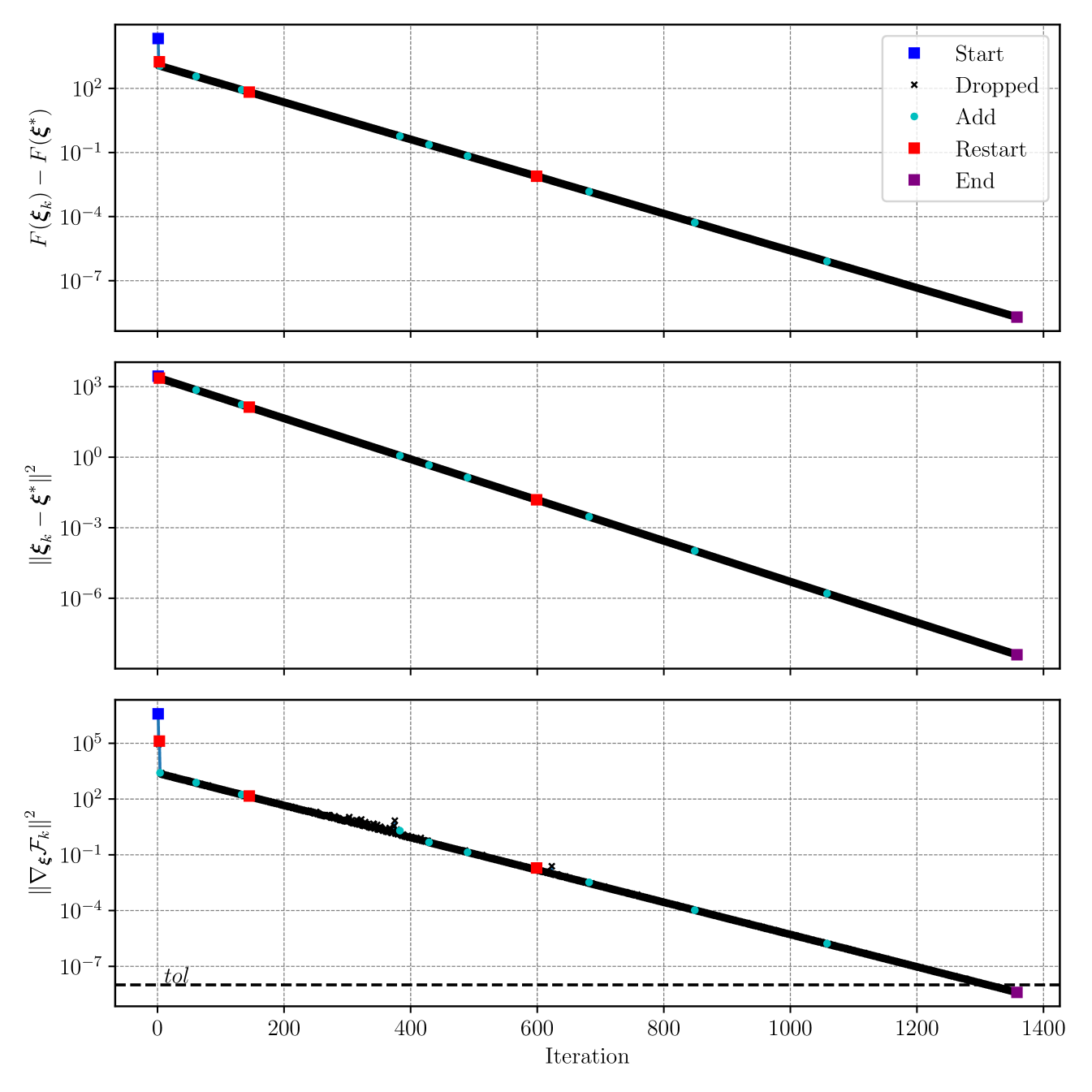
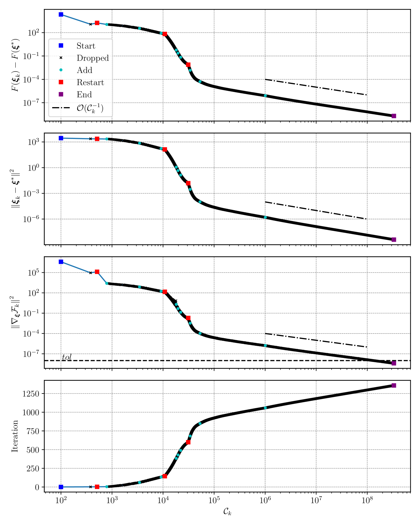
In Figures 1 and 2, we present the optimality gap (131), the squared distance to the optimal point and the squared norm of the gradient estimate versus iteration and number of gradient sampling cost, respectively. In Figure 2 we also plot the iteration reached versus gradient sampling cost. We mark the starting points, restarts, and ending points with blue, red, and purple squares, respectively; the dropped points with black $\times$ , and the remaining iterations in the MICE index set with cyan dots. In Figure 1, one can observe that SGD-MICE attains linear convergence with a constant step-size, as predicted in Proposition 2. In Figure 2, we present the convergence plots versus gradient sampling cost, exhibiting numerical rates of $\mathcal{O}(\mathcal{C}_{k}^{-1})$ . These rates are expected as the distance to the optimal point converges linearly (see Proposition 2) and the cost of sampling new gradients per iteration grows as $\mathcal{C}_{k}=\mathcal{O}(\|\nabla F(\boldsymbol{\xi}_{k})\|^{-2})$ , as shown in (30). Note that the convergence is exponential as in the deterministic case until around $4\times 10^{4}$ gradient evaluations. After this point, there is a change of regime in which we achieve the asymptotic rates; after $4\times 10^{4}$ , the cost of performing each iteration grows exponentially.

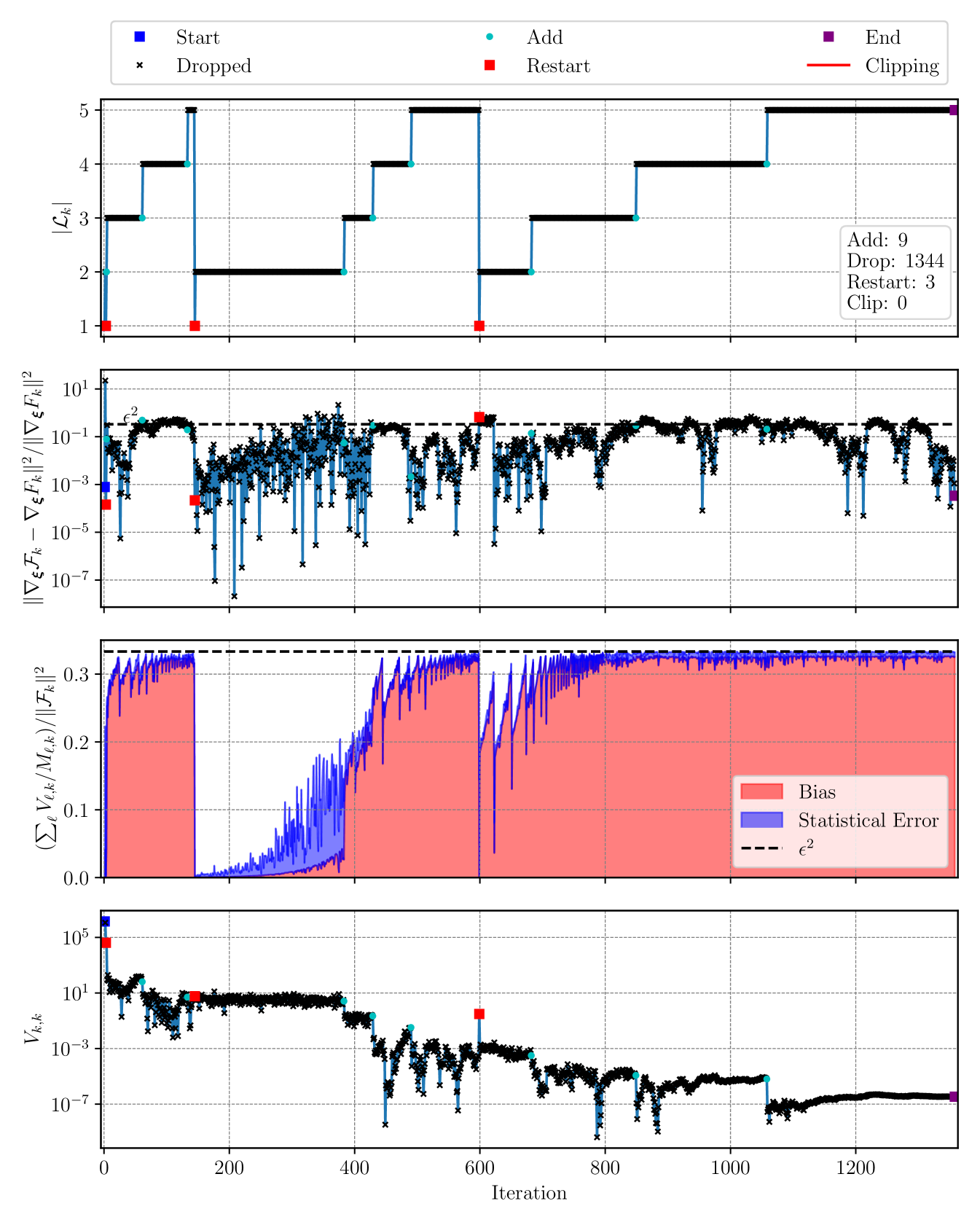
Figure 3 presents the cardinality of the index set $\mathcal{L}_{k}$ , the true squared relative $L^{2}$ error, an approximation of the error that we control to be less than $\epsilon$ , and $V_{k,k}$ versus iteration. Moreover, on the relative error plots, horizontal lines with the upper bounds we impose are presented. It can be seen that imposing the condition $\sum_{\ell\in\mathcal{L}_{k}}V_{\ell,k}/M_{\ell,k}\leq\epsilon^{2}\left\|\nabla\mathcal{F}_{k}\right\|^{2}$ results in the actual relative squared error being below $\epsilon$ . Also, we split the empirical relative error between bias and statistical error, as discussed in Appendix B. Note that the bias is reset when MICE’s index set is restarted. The $V_{k,k}$ plot illustrates how the variance of the last gradient difference decreases with the optimization, notably when a new element is added to the set $\mathcal{L}_{k}$ .

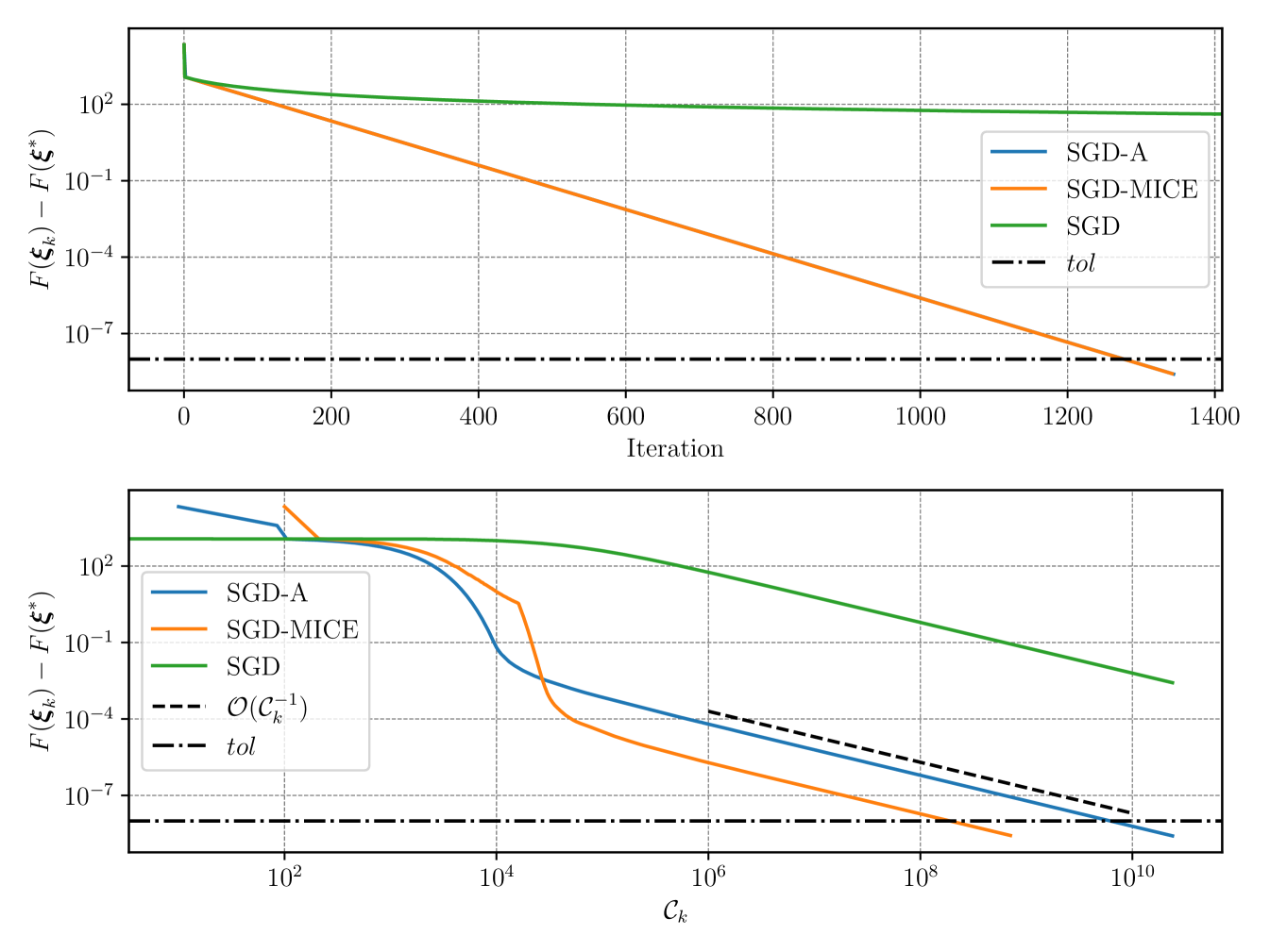
To validate the robustness and performance increase of SGD-MICE, we compare it with SGD using Monte Carlo sampling, at every iteration, to estimate the mean gradient, which we call SGD-A. Likewise, SGD-MICE, SGD-A controls the relative error in the mean gradient approximation. In practice, SGD-A is SGD-MICE but only equipped with the Restart index set operator. We run both methods until the tolerance $tol=10^{-8}$ is reached. Then, we run vanilla SGD (Robbins–Monro algorithm [31]) with sample size $1000$ until it reaches the same work as SGD-A.

In Figure 4, we present the optimality gap per iteration and number of gradient evaluations for SGD-A, SGD-MICE, and vanilla SGD. Our SGD-MICE achieved the desired tolerance with $3\%$ of the cost needed by SGD-A, illustrating the performance improvement of using the data from previous iterations efficiently.

Although this example is very simple, it illustrates the performance of SGD-MICE in an ideal situation where both $L$ and $\mu$ are known. Finally, SGD-MICE was able to automatically decide whether to drop iterations, restart, or clip the index set to minimize the overall work required to attain the linear convergence per iteration.

Refer to caption — Figure 1. Single run, random quadratic example, Equation (134) with $\kappa=100$ . Optimality gap (top), squared distance to the optimal point (center), and squared norm of gradient estimate (bottom) per iteration for SGD-MICE. The starting point, the restarts, and the end are marked respectively as blue, red, and purple squares, iterations dropped with black $\times$ , and the remaining MICE points with cyan circles. SGD-MICE is able to achieve linear $L^{2}$ convergence as predicted in Proposition 2.

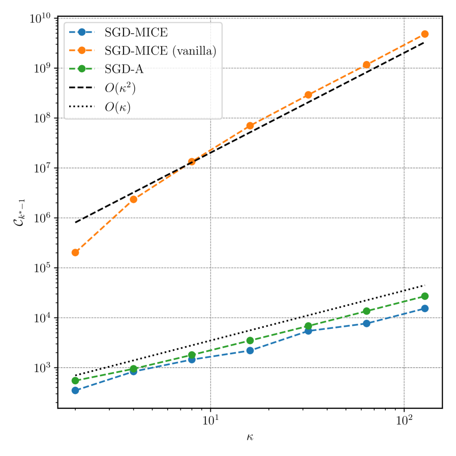
In §3.2, we prove that, for expectation minimization, the gradient sampling cost necessary to reach a certain $\left\|\nabla_{\boldsymbol{\xi}}F(\xi_{k^{*}})\right\|^{2}<tol$ is $\mathcal{O}\left(\kappa^{2}tol^{-1}\right)$ for SGD-MICE and $\mathcal{O}\left(\kappa tol^{-1}\log(tol^{-1})\right)$ for SGD-A. To validate numerically the dependency of the cost with respect to the conditioning number, we evaluated both SGD-MICE and SGD-A with different condition numbers until the stopping criterion. Moreover, we also tested SGD-MICE with and without the index set operators Restart, Drop, and Clip. The reasoning for doing this test is that, in the analysis of Corollary 4, we consider the case where all iterates are kept in the index set. However, in practice, one would expect SGD-MICE with the index set operators to perform better than both vanilla SGD-MICE (without the operators) and SGD-A; in one extreme case where all iterates are kept, we recover vanilla SGD-MICE, and in another extreme case we restart every iteration, resulting in SGD-A. The gradient sampling cost versus $\kappa$ for these tests is presented in Figure 5.

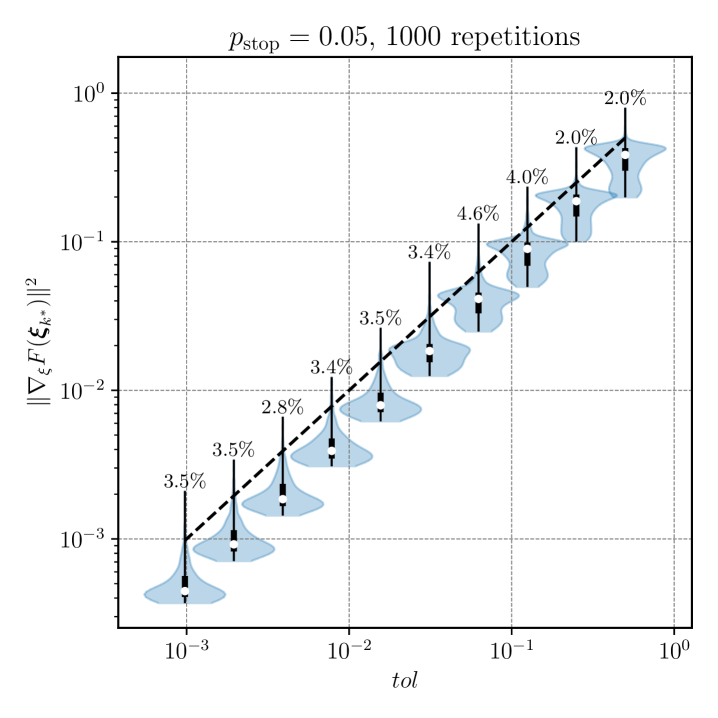
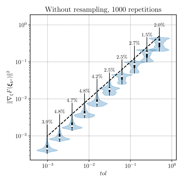
In Remark 6, we present a resampling technique to take more informed decisions on stopping criterion and error control. To validate our stopping criterion, we performed a thousand independent runs of SGD-MICE for different values of $tol$ , using the resampling to decide both sample sizes and the stopping criterion. Figure 6 presents violin plots with approximations of empirical distributions of the squared gradient norms where optimization stopped and the percentage of times this quantity exceeded $tol$ . Moreover, we show both the case where we use the resampling technique and when we do not use it. For lower tolerances, the resampling technique indeed reduced the percentage of premature stops, however, in both cases, a general trend of decrease following $tol$ is observed.

5.2. Stochastic Rosenbrock function

The goal of this example is to test the performance of Adam-MICE, that is, Adam coupled with our gradient estimator MICE, in minimizing the expected value of the stochastic Rosenbrock function in (138), showing that MICE can be coupled with different first-order optimization methods in a non-intrusive manner. Here we adapt the deterministic Rosenbrock function to the stochastic setting, specializing our optimization problem (1) with

(137)

f(\boldsymbol{\xi},\boldsymbol{\theta})=\left(a-\xi_{0}+\theta_{0}\right)^{2}+b\left(-\xi_{0}^{2}+\xi_{1}+\theta_{0}^{2}-\theta_{1}^{2}\right)^{2},

where $a=1$ , $b=100$ , $\theta_{0},\theta_{1}\sim\mathcal{N}(0,\sigma_{\theta}^{2})$ . The objective function to be minimized is thus

(138)

F(\boldsymbol{\xi})=(a-\xi_{0})^{2}+\sigma_{\theta}^{2}+b\left(4\sigma_{\theta}^{4}+(\xi_{1}-\xi_{0}^{2})^{2}\right),

and its gradient is given by

(139)

\nabla_{\boldsymbol{\xi}}F(\boldsymbol{\xi})=\begin{bmatrix}-2a+4b\xi_{0}^{3}-4b\xi_{0}\xi_{1}+2\xi_{0}\\ -2b\xi_{0}^{2}+2b\xi_{1}\end{bmatrix},

which coincides with the gradient of the deterministic Rosenbrock function. Therefore, the optimal point of the stochastic Rosenbrock is the same as the one of the deterministic: $\boldsymbol{\xi}^{*}=(a,a^{2})$ . To perform the optimization, we sample the stochastic gradient

(140)

\nabla_{\boldsymbol{\xi}}f(\boldsymbol{\xi},\boldsymbol{\theta})=\begin{bmatrix}-2a+4b\xi_{0}\left(\xi_{0}^{2}-\xi_{1}-\theta_{0}^{2}+\theta_{1}^{2}\right)+2\xi_{0}-2\theta_{0}\\ 2b\left(-\xi_{0}^{2}+\xi_{1}+\theta_{0}^{2}-\theta_{1}^{2}\right)\end{bmatrix}.

Although this is still a low dimensional example, minimizing the Rosenbrock function poses a difficult optimization problem for first-order methods; these tend to advance slowly in the region where the gradient has near-zero norm. Moreover, when noise is introduced in gradient estimates, their relative error can become large, affecting the optimization convergence.

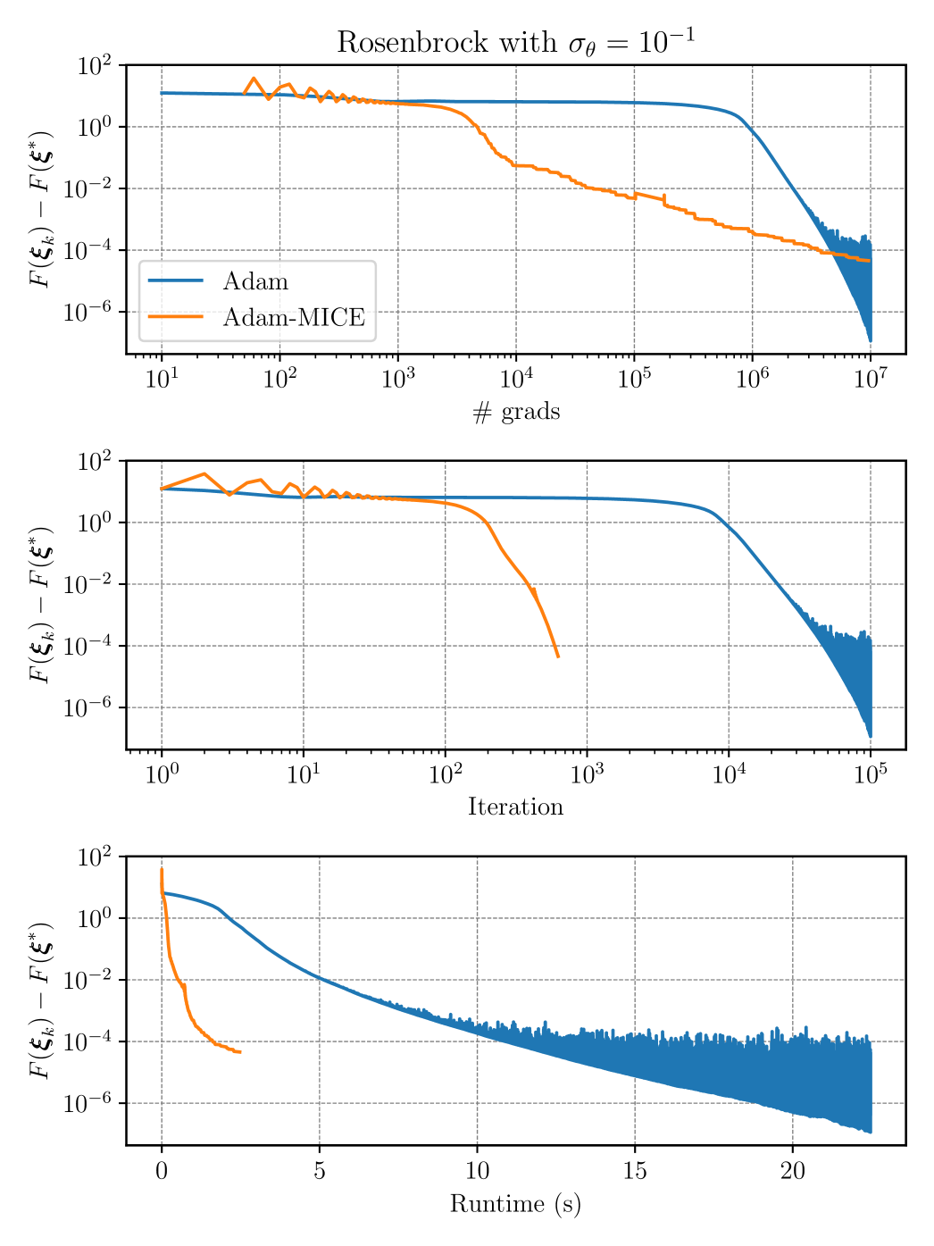
We compare the convergence of the classical Adam algorithm against Adam-MICE. To illustrate the effect of the dispersion of the random variable $\boldsymbol{\theta}$ , two distinct noise levels are considered, namely $\sigma_{\theta}=10^{-4}$ and $\sigma_{\theta}=10^{-1}$ . As for the optimization setup, we set Adam-MICE with fixed step-size $0.3$ and Adam with a decreasing step-size $\eta_{k}=0.01/\sqrt{k}$ , which we observed to be the best step-sizes for each method. The stopping criterion for both algorithms is set as $10^{7}$ gradient evaluations. For Adam-MICE, we use $\epsilon=1.$ , whereas for Adam we use a fixed batch size of $100$ . In all cases, we start the optimization from $\boldsymbol{\xi}_{0}=(-1.5,2.5)$

In Figures 7 and 8, we present, for $\sigma_{\theta}$ of $10^{-1}$ and $10^{-4}$ , respectively, the optimality gap for both Adam and Adam-MICE versus the number of gradients, iterations, and runtime in seconds. It is clear that Adam-MICE is more stable than Adam as the latter oscillates as it approximates the optimal point in both cases. The efficient control of the error in gradient estimates allows Adam-MICE to converge monotonically in the asymptotic phase. Moreover, the number of iterations and the runtime are much smaller for Adam-MICE than for Adam.

As a conclusion, even though Adam has its own mechanisms to control the statistical error of gradients, coupling it with MICE, for this example, has proven to be advantageous as it allows more evaluations to be performed simultaneously. Moreover, as the gradient error is controlled, we can use Adam with a fixed step-size. Also, MICE allows for a stopping criterion based on the gradient norm, which would not be possible for vanilla Adam.

5.3. Logistic regression

In this example, we train logistic regression models using SGD-MICE, SAG [46], SAGA [26], SARAH [23], and SVRG [22] to compare their performances. Here, we present a more practical application of MICE, where we can test its performance on high-dimensional settings with finite populations. Therefore, we calculate the error as in (2) and use Algorithm 1 to obtain the optimal sample sizes. To train the logistic regression model for binary classification, we use the $\ell_{2}$ -regularized log-loss function

(141)

F(\boldsymbol{\xi})=\frac{1}{N}\sum_{i=1}^{N}f\left(\boldsymbol{\xi},\boldsymbol{\theta}_{i}=(\boldsymbol{x}_{i},y_{i})\right)=\frac{1}{N}\sum_{i=1}^{N}\log(1+\exp(-y_{i}\boldsymbol{\xi}\cdot\boldsymbol{x}_{i}))+\frac{\lambda}{2}\|\boldsymbol{\xi}\|^{2},

where each data point $(\boldsymbol{x}_{i},y_{i})$ is such that $\boldsymbol{x}_{i}\in\mathbb{R}^{d_{\boldsymbol{\xi}}}$ and $y_{i}\in\{-1,1\}$ . We use the datasets mushrooms, gisette, and Higgs, obtained from LibSVM¹¹1 https://www.csie.ntu.edu.tw/~cjlin/libsvmtools/datasets/binary.html . The size of the datasets $N$ , number of features $d_{\boldsymbol{\xi}}$ , and regularization parameters $\lambda$ are presented in Table 1.

Table 1. Size, number of features, and regularization parameters for the datasets used in the logistic regression example.

Dataset	Size	Features	$\lambda$	$\kappa$
mushrooms	8124	112	$10^{-5}$	12316.30
gisette	6000	5000	$10^{-4}$	1811.21
HIGGS	11000000	28	$10^{-4}$	765.76

When using SGD-MICE for training the logistic regression model, we use $\epsilon=1/\sqrt{3}$ . For the other methods, we use batch sizes of size $10$ . Since we have finite populations, we use Algorithm 1 to calculate the sample-sizes. SGD-MICE step is based on the Lipschitz smoothness of the true objective function as presented in Proposition 2. Conversely, the other methods rely on a Lipschitz constant that must hold for all data points, which we refer to as $\hat{L}$ . A maximum index set cardinality of $100$ is imposed on SGD-MICE; if $|\mathcal{L}_{k}|=100$ , we restart the index set. The step-sizes for SAG, SAGA, SARAH, and SVRG are presented in Table 2. These steps were chosen as the best performing for each case based on the recommendations of their original papers.

Table 2. Step-sizes chosen for each method for the logistic regression example.

Method	SAG	SAGA	SARAH	SVRG
Step-size	$\frac{1}{16(\hat{L}+\mu N)}$	$\frac{1}{2(\hat{L}+\mu N)}$	$\frac{1}{2\hat{L}}$	$\frac{1}{2\hat{L}}$

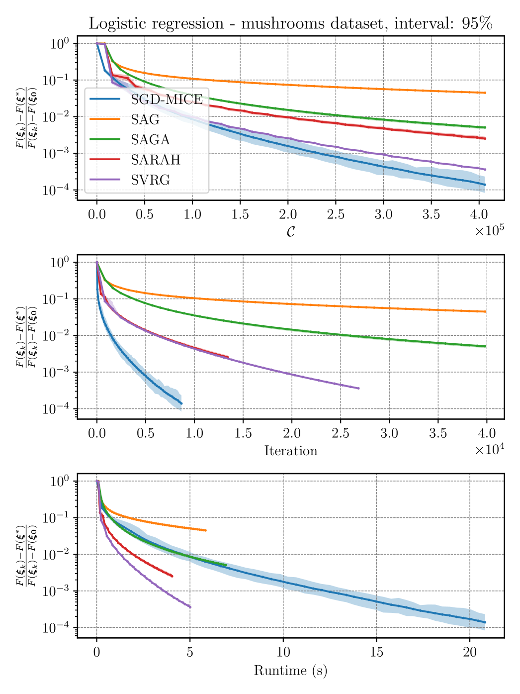
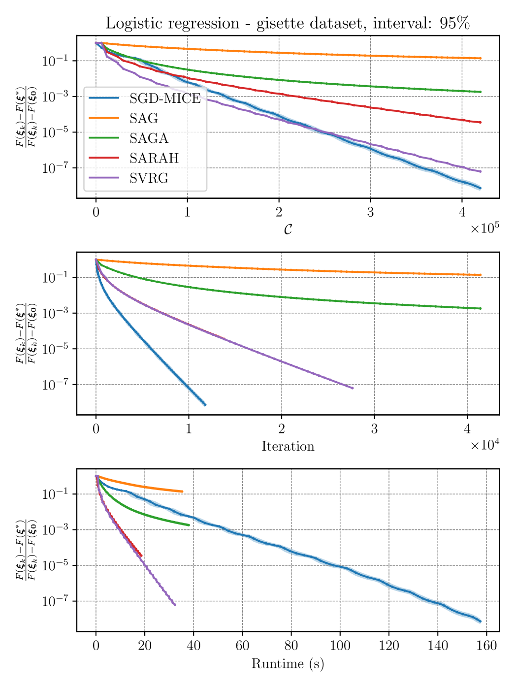
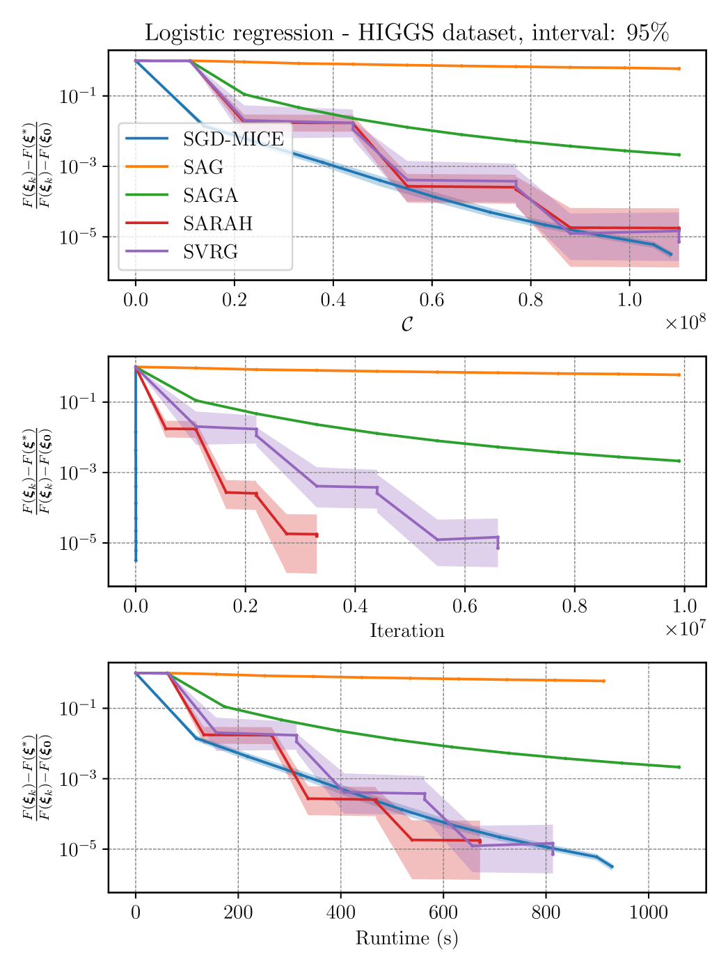
To evaluate the consistency of SGD-MICE versus the other baseline methods, we perform $100$ independent runs of each method for each dataset. Figures 9, 10, and 11 present confidence intervals and median of the relative optimality gap (the optimality gap normalized by its starting value) for, respectively, the mushrooms, gisette, and HIGGS datasets versus the number of gradient evaluations, iterations and runtime in seconds.

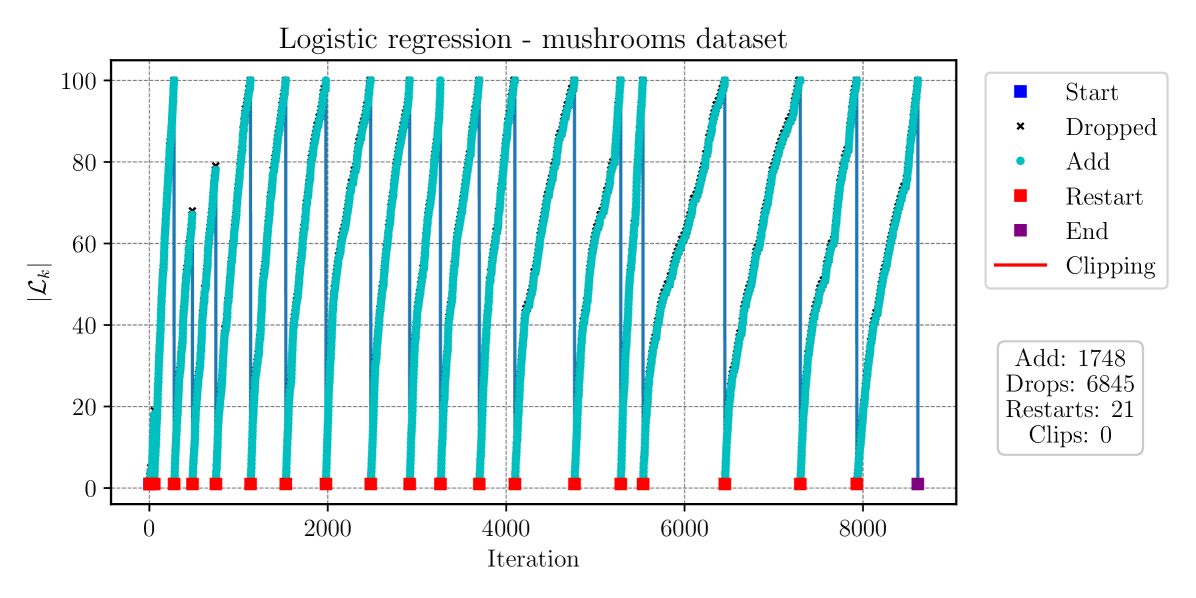
In the mushrooms dataset, SGD-MICE decreases the optimality gap more than the other methods for the same number of gradient samples during the whole optimization process. Moreover, the total number of iterations is much smaller than for the other methods. Yet, the overhead of our SGD-MICE implementation becomes clear when we compare the runtimes; the current implementation of SGD-MICE is more costly than the other methods. In the gisette dataset, SGD-MICE shows a better convergence rate when compared to the other methods, both in terms of number of gradient evaluations as in iterations. The overhead, however, is significantly larger, due to the larger number of optimization variables here, $5000$ . Finally, for the HIGGS dataset, which is a much larger dataset, SGD-MICE performs better than the other methods in the number of gradient evaluations, iterations, and is competitive with SARAH and SVRG in runtime. Moreover, on average SGD-MICE performed $2179$ iterations while the other methods required more than $10^{6}$ iterations. Thus, more gradient evaluations can be performed simultaneously in parallel. Figure 12 presents the index set cardinalities versus iterations of SGD-MICE for the three datasets. Moreover, we present the iterations that were kept in the index set, the ones that were dropped, as well as restarts and clippings.

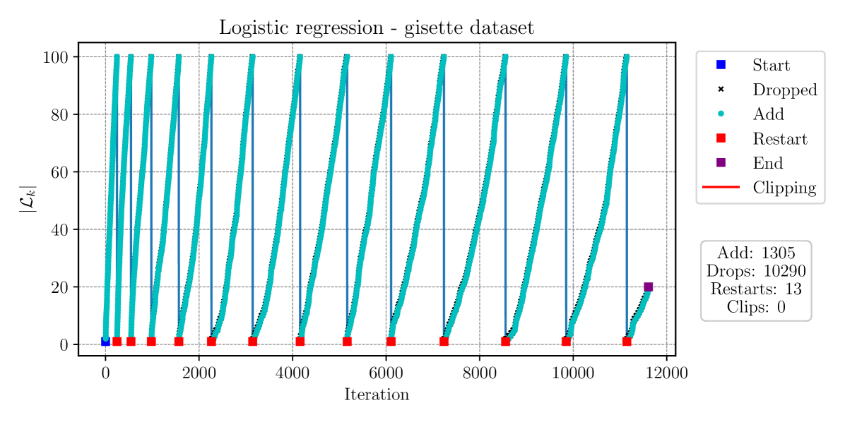
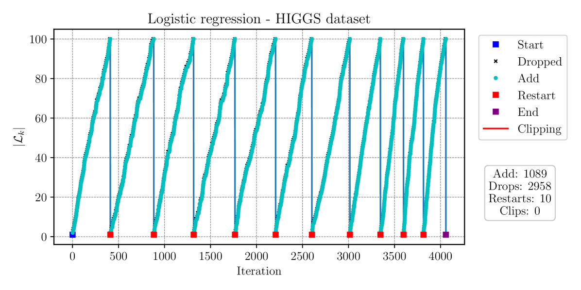
From the results of this example, we observe that MICE performs well in problems with a reasonably large number of parameters, for instance, $5000$ in the gisette, and finite dataset populations ranging from the thousands to the millions. One can conclude from the results obtained that SGD-MICE’s performance compared to the other methods increases as the population size grows. Note that both SAG and SAGA need to decrease their step-sizes as the sample-size increases, and that SARAH and SVRG need to reevaluate the full-gradient after a few epochs to keep their convergence.

6. Acknowledgments

This publication is based upon work supported by the King Abdullah University of Science and Technology (KAUST) Office of Sponsored Research (OSR) under Award No. OSR-2019-CRG8-4033, the Alexander von Humboldt Foundation, and Coordination for the Improvement of Higher Education Personnel (CAPES).

Last but not least, we want to thank Dr. Sören Wolfers and Prof. Jesper Oppelstrup. They both provided us with valuable ideas and constructive comments.

7. Conflict of interest

The authors have no conflicts to disclose.

8. Data Availability

The data that support the findings of this study are available from the corresponding author upon reasonable request. A python implementation of MICE can be found at PyPi https://pypi.org/project/mice/. We use the datasets mushrooms, gisette, and Higgs, obtained from LibSVM https://www.csie.ntu.edu.tw/~cjlin/libsvmtools/datasets/binary.html.

9. Conclusion

We introduced the Multi-Iteration Stochastic Optimizers, a novel class of first-order stochastic optimization methods that use the Multi-Iteration stochastiC Estimator (MICE). The MICE estimator utilizes successive control variates along optimization paths, efficiently reusing previously computed gradients to achieve accurate mean gradient approximations. At each iteration, it adaptively samples gradients to satisfy a user-specified relative error tolerance. Moreover, it employs a greedy strategy to determine which iterates to retain in memory and which to discard.

Thanks to its ability to control relative gradient error, MICE facilitates robust stopping criteria based on the gradient norm. Moreover, its nonintrusive design makes it readily integrable with existing first-order optimization methods, significantly expanding its applicability.

We provided a rigorous theoretical analysis for SGD-MICE, highlighting its strong performance across different classes of optimization problems. In particular, we proved exponential convergence in the $L^{2}$ sense for gradient-dominated functions under constant step-size conditions. For strongly convex problems, our results demonstrate that SGD-MICE achieves accuracy $tol$ with an average complexity of $\mathcal{O}(tol^{-1})$ gradient evaluations, outperforming conventional adaptive batch-size SGD methods, which require $\mathcal{O}(tol^{-1}\log(tol^{-1}))$ evaluations.

Numerically, we validated our theory through three illustrative examples, employing consistent MICE parameters across diverse scenarios. The tests ranged from a quadratic function with stochastic Hessian to a stochastic Rosenbrock problem solved via Adam-MICE, and finally logistic regression training on large-scale datasets. In the latter, SGD-MICE demonstrated competitive performance against established variance-reduction methods (SAG, SAGA, SVRG, and SARAH), confirming its practical efficiency and scalability.

Future research directions include extending MICE to quasi-Newton methods, exploring constrained optimization settings through standard techniques like projected gradients and active set methods, and investigating additional gradient estimation error sources, such as biases from numerical discretizations.

References

[1] K. Marti. Stochastic optimization methods, volume 2. Springer, 2005.
[2] S. Uryasev and P.M. Pardalos. Stochastic optimization: algorithms and applications, volume 54. Springer Science & Business Media, 2013.
[3] J.R. Birge and F. Louveaux. Introduction to Stochastic Programming. Springer Publishing Company, Incorporated, 2nd edition, 2011.
[4] G. Lan. First-order and Stochastic Optimization Methods for Machine Learning. Springer, 2020.
[5] S.W. Wallace and W.T. Ziemba. Applications of stochastic programming. SIAM, 2005.
[6] W.H. Fleming and R.W. R. Deterministic and stochastic optimal control, volume 1. Springer Science & Business Media, 2012.
[7] W.T. Ziemba and R.G. Vickson. Stochastic optimization models in finance. Academic Press, 2014.
[8] A.J. Conejo, M. Carrión, J.M. Morales, et al. Decision making under uncertainty in electricity markets, volume 1. Springer, 2010.
[9] C. Bayer, R. Tempone, and S. Wolfers. Pricing American options by exercise rate optimization. Quant. Finance, 20(11):1749–1760, 2020.
[10] F.-R. Chang. Stochastic optimization in continuous time. Cambridge University Press, 2004.
[11] P. Azcue and N. Muler. Stochastic optimization in insurance. SpringerBriefs in Quantitative Finance. Springer, New York, 2014. A dynamic programming approach.
[12] Z. Ding. Stochastic Optimization and Its Application to Communication Networks and the Smart Grid. University of Florida Digital Collections. University of Florida, 2012.
[13] D.D. Yao, H. Zhang, and X.Y. Zhou, editors. Stochastic modeling and optimization. Springer-Verlag, New York, 2003. With applications in queues, finance, and supply chains.
[14] E.G. Ryan, C.C. Drovandi, J.M. McGree, and A.N. Pettitt. A review of modern computational algorithms for bayesian optimal design. International Statistical Review, 84(1):128–154, 2016.
[15] A.G. Carlon, B.M. Dia, L. Espath, R.H. Lopez, and R. Tempone. Nesterov-aided stochastic gradient methods using laplace approximation for bayesian design optimization. Computer Methods in Applied Mechanics and Engineering, 363, 2020.
[16] S. Heinrich. The multilevel method of dependent tests. In Advances in stochastic simulation methods, pages 47–61. Springer, 2000.
[17] M.B. Giles. Multilevel Monte Carlo path simulation. Operations research, 56(3):607–617, 2008.
[18] D. Ruppert. Efficient estimations from a slowly convergent robbins-monro process. Technical report, Cornell University Operations Research and Industrial Engineering, 1988.
[19] R.H. Byrd, G.M. Chin, J. Nocedal, and Y. Wu. Sample size selection in optimization methods for machine learning. Mathematical programming, 134(1):127–155, 2012.
[20] L. Balles, J. Romero, and P. Hennig. Coupling adaptive batch sizes with learning rates. arXiv preprint arXiv:1612.05086, 2016.
[21] R. Bollapragada, R. Byrd, and J. Nocedal. Adaptive sampling strategies for stochastic optimization. SIAM Journal on Optimization, 28(4):3312–3343, 2018.
[22] R. Johnson and T. Zhang. Accelerating stochastic gradient descent using predictive variance reduction. In Advances in neural information processing systems, pages 315–323, 2013.
[23] L.M. Nguyen, J. Liu, K. Scheinberg, and M. Takáč. Sarah: A novel method for machine learning problems using stochastic recursive gradient. In Proceedings of the 34th International Conference on Machine Learning-Volume 70, pages 2613–2621. JMLR. org, 2017.
[24] L. Nguyen, K. Scheinberg, and M. Takáč. Inexact sarah algorithm for stochastic optimization. Optimization methods & software, 08 2020.
[25] C. Fang, C.J. Li, Z. Lin, and T. Zhang. Spider: Near-optimal non-convex optimization via stochastic path-integrated differential estimator. In Advances in Neural Information Processing Systems, pages 689–699, 2018.
[26] A. Defazio, F. Bach, and S. Lacoste-Julien. Saga: A fast incremental gradient method with support for non-strongly convex composite objectives. In Advances in neural information processing systems, pages 1646–1654, 2014.
[27] M.P. Friedlander and M. Schmidt. Hybrid deterministic-stochastic methods for data fitting. SIAM Journal on Scientific Computing, 34(3):A1380–A1405, 2012.
[28] S. De, A. Yadav, D. Jacobs, and T. Goldstein. Big batch sgd: Automated inference using adaptive batch sizes. arXiv preprint arXiv:1610.05792, 2016.
[29] K. Ji, Z. Wang, Y. Zhou, and Y. Liang. Faster stochastic algorithms via history-gradient aided batch size adaptation. arXiv preprint arXiv:1910.09670, 2019.
[30] B. T Polyak. Introduction to optimization. optimization software. Inc., Publications Division, New York, 1, 1987.
[31] H. Robbins and S. Monro. A stochastic approximation method. The annals of mathematical statistics, pages 400–407, 1951.
[32] D. P Kingma and J. Ba. Adam: A method for stochastic optimization. arXiv preprint arXiv:1412.6980, 2014.
[33] J.C. Spall. Introduction to stochastic search and optimization: estimation, simulation, and control, volume 65. John Wiley & Sons, 2005.
[34] A. Shapiro, D. Dentcheva, and A. Ruszczyński. Lectures on stochastic programming: modeling and theory. SIAM, 2014.
[35] A. Nitanda. Stochastic proximal gradient descent with acceleration techniques. In Advances in Neural Information Processing Systems, pages 1574–1582, 2014.
[36] J. Konečnỳ, J. Liu, P. Richtárik, and M. Takáč. Mini-batch semi-stochastic gradient descent in the proximal setting. IEEE Journal of Selected Topics in Signal Processing, 10(2):242–255, 2016.
[37] S. Heinrich. Multilevel Monte Carlo methods. In Large-Scale Scientific Computing, volume 2179 of Lecture Notes in Computer Science, pages 58–67. Springer Berlin Heidelberg, 2001.
[38] M.B. Giles. Multilevel monte carlo methods. Acta Numerica, 24:259–328, 2015.
[39] S. Dereich and T. Müller-Gronbach. General multilevel adaptations for stochastic approximation algorithms of Robbins-Monro and Polyak-Ruppert type. Numer. Math., 142(2):279–328, 2019.
[40] S. Yang, M. Wang, and E.X. Fang. Multilevel stochastic gradient methods for nested composition optimization. SIAM Journal on Optimization, 29(1):616–659, 2019.
[41] A. C. Davison and D. V. Hinkley. Bootstrap methods and their application. Number 1. Cambridge university press, 1997.
[42] H. Karimi, J. Nutini, and M. Schmidt. Linear convergence of gradient and proximal-gradient methods under the polyak-łojasiewicz condition. In Joint European conference on machine learning and knowledge discovery in databases, pages 795–811. Springer, 2016.
[43] Y. Nesterov. Lectures on convex optimization, volume 137. Springer, 2018.
[44] B. Efron. The jackknife, the bootstrap, and other resampling plans, volume 38. Siam, 1982.
[45] B.P. Welford. Note on a method for calculating corrected sums of squares and products. Technometrics, 4(3):419–420, 1962.
[46] M. Schmidt, N. Le Roux, and F. Bach. Minimizing finite sums with the stochastic average gradient. Mathematical Programming, 162(1-2):83–112, 2017.

Appendix A Multi-iteration stochastic optimizers

In this section, we present the detailed algorithms for the multi-iteration stochastic optimizers using the MICE estimator for the mean gradient. In Algorithms 4, 5, we respectively describe the pseudocodes for SGD-MICE and Adam-MICE.

Algorithm 4 Pseudocode for SGD-MICE with fixed step-size. SGD-MICE requires an unbiased estimator of the true gradient,

\nabla f

; a distribution from which

\boldsymbol{\theta}

can be sampled,

\pi

; a starting point,

\boldsymbol{\xi}_{0}

; and a tolerance on the squared gradient norm,

tol

1:procedure SGD-MICE(

\nabla_{\boldsymbol{\xi}}f

\pi

\boldsymbol{\xi}_{0}

tol

)

k\leftarrow 0

3: while

\left\|\nabla_{\boldsymbol{\xi}}\mathcal{F}_{k}^{\text{stop}}\right\|^{2}>tol

\triangleright

\left\|\nabla_{\boldsymbol{\xi}}\mathcal{F}_{k}^{\text{stop}}\right\|

computed as in Remark 6

4: Evaluate

\nabla_{\boldsymbol{\xi}}\mathcal{F}_{k}

using Algorithm 2

\boldsymbol{\xi}_{k+1}\leftarrow\boldsymbol{\xi}_{k}-\eta\nabla_{\boldsymbol{\xi}}\mathcal{F}_{k}

k\leftarrow k+1

7: end while

8: return optimum approximation

\boldsymbol{\xi}_{k^{*}}

9:end procedure

Algorithm 5 Pseudocode for Adam-MICE with fixed step-size. Adam-MICE requires an unbiased estimator of the true gradient,

\nabla f

; a distribution from which

\boldsymbol{\theta}

can be sampled,

\pi

; a starting point,

\boldsymbol{\xi}_{0}

; and a tolerance on the squared gradient norm,

tol

. Moreover, Adam-MICE requires the constants

\beta_{1}

\beta_{2}

, and

\epsilon_{\text{Adam}}

. We use the values recommended by [32],

\beta_{1}=0.9

\beta_{2}=0.999

, and

\epsilon_{\text{Adam}}=10^{-8}

1:procedure Adam-MICE(

\nabla_{\boldsymbol{\xi}}f

\pi

\boldsymbol{\xi}_{0}

tol

)

2: Initialize

\boldsymbol{m}_{0}

and

\boldsymbol{v}_{0}

as zero-vectors

k\leftarrow 0

4: while

\left\|\nabla_{\boldsymbol{\xi}}\mathcal{F}_{k}^{\text{stop}}\right\|^{2}>tol

\triangleright

\left\|\nabla_{\boldsymbol{\xi}}\mathcal{F}_{k}^{\text{stop}}\right\|

computed as in Remark 6

5: Evaluate

\nabla_{\boldsymbol{\xi}}\mathcal{F}_{k}

using Algorithm 2

\boldsymbol{m}_{k}\leftarrow\beta_{1}\boldsymbol{m}_{k-1}+(1-\beta_{1})\nabla_{\boldsymbol{\xi}}\mathcal{F}_{k}

\boldsymbol{v}_{k}\leftarrow\beta_{2}\boldsymbol{v}_{k-1}+(1-\beta_{2})\nabla_{\boldsymbol{\xi}}\mathcal{F}_{k}^{2}

\triangleright

The gradient estimates are squared element-wise

\boldsymbol{\hat{m}}_{k}\leftarrow\boldsymbol{m}_{k-1}/(1-\beta_{1}^{k+1})

\boldsymbol{\hat{v}}_{k}\leftarrow\boldsymbol{v}_{k-1}/(1-\beta_{2}^{k+1})

10:

\boldsymbol{\xi}_{k+1}\leftarrow\boldsymbol{\xi}_{k}-\eta\boldsymbol{\hat{m}}_{k}/(\sqrt{\boldsymbol{\hat{v}}_{k}}+\epsilon_{\text{Adam}})

11:

k\leftarrow k+1

12: end while

13: return optimum approximation

\boldsymbol{\xi}_{k^{*}}

14:end procedure

Adapting stochastic optimization algorithms to use MICE is as straight-forward as substituting the gradient estimator and the stopping criterion, as can be seen in Algorithms 4 and 5.

Appendix B Error decomposition of the MICE estimator

The MICE estimator has a conditional bias due to the reuse of previous information. Here we prove that, if the statistical error of the estimator is controlled every iteration, then the bias is implicitly controlled as well. Recall the MICE estimator is defined as

(142)

\nabla\mathcal{F}_{k}=\sum_{\ell\in\mathcal{L}_{k}}\frac{1}{M_{\ell,k}}\sum_{\alpha\in\mathcal{I}_{\ell,k}}\Delta_{\ell,k,\alpha},

where

(143)

\Delta_{\ell,k,\alpha}=\begin{cases}\nabla f(\boldsymbol{\xi}_{\ell},\boldsymbol{\theta}_{\alpha})-\nabla f(\boldsymbol{\xi}_{p_{k}(\ell)},\boldsymbol{\theta}_{\alpha})&\text{ if }\ell>\min\{\mathcal{L}_{k}\}\\ \nabla f(\boldsymbol{\xi}_{0},\boldsymbol{\theta}_{\alpha})&\text{ if }\ell=\min\{\mathcal{L}_{k}\}.\end{cases}

The squared $L^{2}$ error of the MICE estimator can be decomposed as

(144)

\displaystyle\mathbb{E}\left[\left\|\nabla\mathcal{F}_{k}-\nabla_{\boldsymbol{\xi}}F(\boldsymbol{\xi}_{k})\right\|^{2}\right]

\displaystyle=\underbrace{\mathbb{E}\left[\left\|\nabla\mathcal{F}_{k}-\mathbb{E}\left[\left.\nabla\mathcal{F}_{k}\;\right|\left\{\boldsymbol{\xi}_{\ell^{\prime}}\right\}_{\ell^{\prime}\in\mathcal{L}_{k}}\right]\right\|^{2}\right]}_{\text{statistical error}}+\underbrace{\mathbb{E}\left[\left\|\mathbb{E}\left[\left.\nabla\mathcal{F}_{k}\;\right|\left\{\boldsymbol{\xi}_{\ell^{\prime}}\right\}_{\ell^{\prime}\in\mathcal{L}_{k}}\right]-\nabla_{\boldsymbol{\xi}}F(\boldsymbol{\xi}_{k})\right\|^{2}\right],}_{\text{bias contribution}}

due to

(145)

\mathbb{E}\left[\mathbb{E}\left[\left.\Big{\langle}\nabla\mathcal{F}_{k}-\mathbb{E}\left[\left.\nabla\mathcal{F}_{k}\;\right|\left\{\boldsymbol{\xi}_{\ell^{\prime}}\right\}_{\ell^{\prime}\in\mathcal{L}_{k}}\right],\mathbb{E}\left[\left.\nabla\mathcal{F}_{k}\;\right|\left\{\boldsymbol{\xi}_{\ell^{\prime}}\right\}_{\ell^{\prime}\in\mathcal{L}_{k}}\right]-\nabla_{\boldsymbol{\xi}}F(\boldsymbol{\xi}_{k})\Big{\rangle}\;\right|\left\{\boldsymbol{\xi}_{\ell^{\prime}}\right\}_{\ell^{\prime}\in\mathcal{L}_{k}}\right]\right]\\ =\mathbb{E}\left[\Big{\langle}\underbrace{\mathbb{E}\left[\left.\nabla\mathcal{F}_{k}-\mathbb{E}\left[\left.\nabla\mathcal{F}_{k}\;\right|\left\{\boldsymbol{\xi}_{\ell^{\prime}}\right\}_{\ell^{\prime}\in\mathcal{L}_{k}}\right]\;\right|\left\{\boldsymbol{\xi}_{\ell^{\prime}}\right\}_{\ell^{\prime}\in\mathcal{L}_{k}}\right]}_{=0},\mathbb{E}\left[\left.\nabla\mathcal{F}_{k}\;\right|\left\{\boldsymbol{\xi}_{\ell^{\prime}}\right\}_{\ell^{\prime}\in\mathcal{L}_{k}}\right]-\nabla_{\boldsymbol{\xi}}F(\boldsymbol{\xi}_{k})\Big{\rangle}\right]

Before we analyze the bias and statistical errors, let us analyze the conditional expectation of the MICE estimator,

(146)

\displaystyle\mathbb{E}\left[\left.\nabla\mathcal{F}_{k}\;\right|\left\{\boldsymbol{\xi}_{\ell^{\prime}}\right\}_{\ell^{\prime}\in\mathcal{L}_{k}}\right]

\displaystyle=\sum_{\ell\in\mathcal{L}_{k}}\frac{1}{M_{\ell,k}}\sum_{\alpha\in\mathcal{I}_{\ell,k}}\mathbb{E}\left[\left.\Delta_{\ell,k,\alpha}\;\right|\left\{\boldsymbol{\xi}_{\ell^{\prime}}\right\}_{\ell^{\prime}\in\mathcal{L}_{k}}\right],

and noting that, for $\tilde{k}<k$ , $\Delta_{\ell,\tilde{k},\alpha}|\left\{\boldsymbol{\xi}_{\ell^{\prime}}\right\}_{\ell^{\prime}\in\mathcal{L}_{k}}$ is deterministic,

(147)

\mathbb{E}\left[\left.\Delta_{\ell,\tilde{k},\alpha}\;\right|\left\{\boldsymbol{\xi}_{\ell^{\prime}}\right\}_{\ell^{\prime}\in\mathcal{L}_{k}}\right]=\begin{cases}\Delta_{\ell,\tilde{k},\alpha}&\text{ if }\tilde{k}<k\\ \nabla F(\boldsymbol{\xi}_{\ell})-\nabla F(\boldsymbol{\xi}_{p_{k}(\ell)})&\text{ if }\tilde{k}=k.\end{cases}

Let $\mathcal{L}^{\cap}_{k}=\mathcal{L}_{k}\cap\mathcal{L}_{k-1}$ . Splitting the summands in MICE between the terms computed at $k$ and the previous ones,

(148)

\nabla\mathcal{F}_{k}=\underbrace{\left\{\sum_{\ell\in\mathcal{L}^{\cap}_{k}}\frac{1}{M_{\ell,k}}\sum_{\alpha\in\mathcal{I}_{\ell,k-1}}\Delta_{\ell,k,\alpha}\right\}}_{\text{previously computed}}+\underbrace{\left\{\frac{1}{M_{k,k}}\sum_{\alpha\in\mathcal{I}_{k,k}}\Delta_{k,k,\alpha}+\sum_{\ell\in\mathcal{L}^{\cap}_{k}}\frac{1}{M_{\ell,k}}\sum_{\alpha\in\mathcal{I}_{\ell,k}\setminus\mathcal{I}_{\ell,k-1}}\Delta_{\ell,k,\alpha}\right\}}_{\text{computed at $k$}},

taking the expectation conditioned on $\left\{\boldsymbol{\xi}_{\ell^{\prime}}\right\}_{\ell^{\prime}\in\mathcal{L}_{k}}$ , and using $\nabla F(\boldsymbol{\xi}_{p_{k}(\min\{\mathcal{L}_{k}\})})=0$ ,

(151)	$\displaystyle\mathbb{E}\left[\left.\nabla\mathcal{F}_{k}\;\right\|\left\{\boldsymbol{\xi}_{\ell^{\prime}}\right\}_{\ell^{\prime}\in\mathcal{L}_{k}}\right]$	$\displaystyle=\!\begin{multlined}\sum_{\ell\in\mathcal{L}^{\cap}_{k}}\frac{1}{M_{\ell,k}}\sum_{\alpha\in\mathcal{I}_{\ell,k-1}}\Delta_{\ell,k,\alpha}\\ +\nabla F(\boldsymbol{\xi}_{k})-\nabla F(\boldsymbol{\xi}_{k-1})+\sum_{\ell\in\mathcal{L}^{\cap}_{k}}\frac{M_{\ell,k}-M_{\ell,k-1}}{M_{\ell,k}}(\nabla F(\boldsymbol{\xi}_{\ell})-\nabla F(\boldsymbol{\xi}_{p_{k}(\ell)}))\end{multlined}\sum_{\ell\in\mathcal{L}^{\cap}_{k}}\frac{1}{M_{\ell,k}}\sum_{\alpha\in\mathcal{I}_{\ell,k-1}}\Delta_{\ell,k,\alpha}\\ +\nabla F(\boldsymbol{\xi}_{k})-\nabla F(\boldsymbol{\xi}_{k-1})+\sum_{\ell\in\mathcal{L}^{\cap}_{k}}\frac{M_{\ell,k}-M_{\ell,k-1}}{M_{\ell,k}}(\nabla F(\boldsymbol{\xi}_{\ell})-\nabla F(\boldsymbol{\xi}_{p_{k}(\ell)}))$
(153)		$\displaystyle=\!\begin{multlined}\sum_{\ell\in\mathcal{L}^{\cap}_{k}}\frac{1}{M_{\ell,k}}\sum_{\alpha\in\mathcal{I}_{\ell,k-1}}\Delta_{\ell,k,\alpha}+\nabla F(\boldsymbol{\xi}_{k})-\sum_{\ell\in\mathcal{L}^{\cap}_{k}}\frac{M_{\ell,k-1}}{M_{\ell,k}}(\nabla F(\boldsymbol{\xi}_{\ell})-\nabla F(\boldsymbol{\xi}_{p_{k}(\ell)}))\end{multlined}\sum_{\ell\in\mathcal{L}^{\cap}_{k}}\frac{1}{M_{\ell,k}}\sum_{\alpha\in\mathcal{I}_{\ell,k-1}}\Delta_{\ell,k,\alpha}+\nabla F(\boldsymbol{\xi}_{k})-\sum_{\ell\in\mathcal{L}^{\cap}_{k}}\frac{M_{\ell,k-1}}{M_{\ell,k}}(\nabla F(\boldsymbol{\xi}_{\ell})-\nabla F(\boldsymbol{\xi}_{p_{k}(\ell)}))$
(154)		$\displaystyle=\nabla_{\boldsymbol{\xi}}F(\boldsymbol{\xi}_{k})+\sum_{\ell\in\mathcal{L}^{\cap}_{k}}\frac{M_{\ell,k-1}}{M_{\ell,k}}\hat{\boldsymbol{\mu}}_{\ell,k-1}-\sum_{\ell\in\mathcal{L}^{\cap}_{k}}\frac{M_{\ell,k-1}}{M_{\ell,k}}\boldsymbol{\mu}_{\ell,k-1},$

where in (153) we used $\sum_{\ell\in\mathcal{L}^{\cap}_{k}}(\nabla F(\boldsymbol{\xi}_{\ell})-\nabla F(\boldsymbol{\xi}_{p_{k}(\ell)}))=\nabla_{\boldsymbol{\xi}}F(\boldsymbol{\xi}_{k-1})$ .

Next, we investigate the bias of the MICE estimator conditioned on the current iterate $\boldsymbol{\xi}_{k}$ and its contribution to the squared $L^{2}$ error.

Proposition 3 (Bias of the MICE estimator in expectation minimization).

Let the bias of the MICE estimator be defined as

(155)

\boldsymbol{b}_{k}\coloneqq\mathbb{E}\left[\left.\nabla\mathcal{F}_{k}\;\right|\left\{\boldsymbol{\xi}_{\ell^{\prime}}\right\}_{\ell^{\prime}\in\mathcal{L}_{k}}\right]-\nabla F(\boldsymbol{\xi}_{k}).

Then, the bias is

(156)

\boldsymbol{b}_{k}=\sum_{\ell\in\mathcal{L}^{\cap}_{k}}\frac{M_{\ell,k-1}}{M_{\ell,k}}\left(\hat{\boldsymbol{\mu}}_{\ell,k-1}-\boldsymbol{\mu}_{\ell,k-1}\right),

and its contribution to the squared $L^{2}$ error is

(157)

\displaystyle\mathbb{E}\left[\left\|\boldsymbol{b}_{k}\right\|^{2}\right]

\displaystyle=\mathbb{E}\left[\sum_{\ell\in\mathcal{L}^{\cap}_{k}}\frac{M_{\ell,k-1}}{M_{\ell,k}^{2}}V_{\ell,k-1}\right].

Proof.

Equation (156) follows directly in (154). Now, let’s investigate $\mathbb{E}\left[\left\|\boldsymbol{b}_{k}\right\|^{2}\right]$ .

(158)		$\displaystyle\mathbb{E}\left[\left\\|\boldsymbol{b}_{k}\right\\|^{2}\right]$	$\displaystyle=\mathbb{E}\left[\left\\|\sum_{\ell\in\mathcal{L}^{\cap}_{k}}\frac{M_{\ell,k-1}}{M_{\ell,k}}\left(\hat{\boldsymbol{\mu}}_{\ell,k-1}-\boldsymbol{\mu}_{\ell,k-1}\right)\right\\|^{2}\right]$
(161)		$\displaystyle=$	$\displaystyle\!\begin{multlined}\mathbb{E}\Bigg{[}\sum_{\ell\in\mathcal{L}^{\cap}_{k}}\bigg{(}\frac{M_{\ell,k-1}^{2}}{M_{\ell,k}^{2}}\mathbb{E}\left[\left.\left\\|\hat{\boldsymbol{\mu}}_{\ell,k-1}-\boldsymbol{\mu}_{\ell,k-1}\right\\|^{2}\;\right\|\left\{\boldsymbol{\xi}_{\ell^{\prime}}\right\}_{\ell^{\prime}\in\mathcal{L}_{\ell}}\right]\\ +2\sum_{j\in\mathcal{L}^{\cap}_{k}:j>\ell}\frac{M_{\ell,k-1}}{M_{\ell,k}}\frac{M_{j,k-1}}{M_{j,k}}\mathbb{E}\left[\left.\left\langle\hat{\boldsymbol{\mu}}_{\ell,k-1}-\boldsymbol{\mu}_{\ell,k-1},\hat{\boldsymbol{\mu}}_{j,k-1}-\boldsymbol{\mu}_{j,k-1}\right\rangle\;\right\|\left\{\boldsymbol{\xi}_{\ell^{\prime}}\right\}_{\ell^{\prime}\in\mathcal{L}_{j}}\right]\bigg{)}\Bigg{]}.\end{multlined}\mathbb{E}\Bigg{[}\sum_{\ell\in\mathcal{L}^{\cap}_{k}}\bigg{(}\frac{M_{\ell,k-1}^{2}}{M_{\ell,k}^{2}}\mathbb{E}\left[\left.\left\\|\hat{\boldsymbol{\mu}}_{\ell,k-1}-\boldsymbol{\mu}_{\ell,k-1}\right\\|^{2}\;\right\|\left\{\boldsymbol{\xi}_{\ell^{\prime}}\right\}_{\ell^{\prime}\in\mathcal{L}_{\ell}}\right]\\ +2\sum_{j\in\mathcal{L}^{\cap}_{k}:j>\ell}\frac{M_{\ell,k-1}}{M_{\ell,k}}\frac{M_{j,k-1}}{M_{j,k}}\mathbb{E}\left[\left.\left\langle\hat{\boldsymbol{\mu}}_{\ell,k-1}-\boldsymbol{\mu}_{\ell,k-1},\hat{\boldsymbol{\mu}}_{j,k-1}-\boldsymbol{\mu}_{j,k-1}\right\rangle\;\right\|\left\{\boldsymbol{\xi}_{\ell^{\prime}}\right\}_{\ell^{\prime}\in\mathcal{L}_{j}}\right]\bigg{)}\Bigg{]}.$

Using Lemma 1 and $\mathbb{E}\left[\left.\left\|\hat{\boldsymbol{\mu}}_{\ell,k-1}-\boldsymbol{\mu}_{\ell,k-1}\right\|^{2}\;\right|\left\{\boldsymbol{\xi}_{\ell^{\prime}}\right\}_{\ell^{\prime}\in\mathcal{L}_{\ell}}\right]=V_{\ell,k-1}M_{\ell,k-1}^{-1}$ concludes the proof. ∎

Note from (156) that $\mathbb{E}\left[\boldsymbol{b}_{k}\right]=\boldsymbol{0}$ .

Corollary 8 (Bias of the MICE estimator in finite sum minimization).

The bias $\boldsymbol{b}_{k}$ of the MICE estimator in finite sum minimization is similar to the expectation minimization one, with the consideration of the finite population correction factor,

(162)

\displaystyle\mathbb{E}\left[\left\|\boldsymbol{b}_{k}\right\|^{2}\right]

\displaystyle=\mathbb{E}\left[\sum_{\ell\in\mathcal{L}^{\cap}_{k}}\left(\frac{N-M_{\ell,k-1}}{N}\right)\frac{M_{\ell,k-1}}{M_{\ell,k}^{2}}V_{\ell,k-1}\right].

Proof.

The proof follows exactly as in Proposition 3, except the finite population correction factor is used in the centered second moment of $\hat{\boldsymbol{\mu}}_{\ell,k-1}$ , $\mathbb{E}\left[\left.\left\|\hat{\boldsymbol{\mu}}_{\ell,k-1}-\boldsymbol{\mu}_{\ell,k-1}\right\|^{2}\;\right|\left\{\boldsymbol{\xi}_{\ell^{\prime}}\right\}_{\ell^{\prime}\in\mathcal{L}_{\ell}}\right]=(N-M_{\ell,k-1})N^{-1}V_{\ell,k-1}M_{\ell,k-1}^{-1}$ . ∎

Proposition 4 (Statistical error of the MICE estimator in expectation minimization).

The statistical error of the MICE estimator in the case of expectation minimization is

(163)

\displaystyle\mathbb{E}\left[\left\|\nabla\mathcal{F}_{k}-\mathbb{E}\left[\left.\nabla\mathcal{F}_{k}\;\right|\left\{\boldsymbol{\xi}_{\ell^{\prime}}\right\}_{\ell^{\prime}\in\mathcal{L}_{k}}\right]\right\|^{2}\right]

\displaystyle=\mathbb{E}\left[\sum_{\ell\in\mathcal{L}^{\cap}_{k}}\frac{(M_{\ell,k}-M_{\ell,k-1})V_{\ell,k}}{M_{\ell,k}^{2}}\right]+\mathbb{E}\left[\frac{V_{k,k}}{M_{k,k}}\right]

Proof.

From (144), we can use Lemma 2 and Proposition 3 to get

(164)	$\displaystyle\mathbb{E}\left[\left\\|\nabla\mathcal{F}_{k}-\mathbb{E}\left[\left.\nabla\mathcal{F}_{k}\;\right\|\left\{\boldsymbol{\xi}_{\ell^{\prime}}\right\}_{\ell^{\prime}\in\mathcal{L}_{k}}\right]\right\\|^{2}\right]$	$\displaystyle=\mathbb{E}\left[\left\\|\nabla\mathcal{F}_{k}-\nabla_{\boldsymbol{\xi}}F(\boldsymbol{\xi}_{k})\right\\|^{2}\right]-\mathbb{E}\left[\left\\|\mathbb{E}\left[\left.\nabla\mathcal{F}_{k}\;\right\|\left\{\boldsymbol{\xi}_{\ell^{\prime}}\right\}_{\ell^{\prime}\in\mathcal{L}_{k}}\right]-\nabla_{\boldsymbol{\xi}}F(\boldsymbol{\xi}_{k})\right\\|^{2}\right]$
(165)		$\displaystyle=\mathbb{E}\left[\sum_{\ell\in\mathcal{L}_{k}}\frac{V_{\ell,k}}{M_{\ell,k}}\right]-\mathbb{E}\left[\sum_{\ell\in\mathcal{L}^{\cap}_{k}}\frac{M_{\ell,k-1}}{M_{\ell,k}^{2}}V_{\ell,k-1}\right]$
(166)		$\displaystyle=\mathbb{E}\left[\sum_{\ell\in\mathcal{L}^{\cap}_{k}}\frac{V_{\ell,k}}{M_{\ell,k}}-\sum_{\ell\in\mathcal{L}^{\cap}_{k}}\frac{M_{\ell,k-1}}{M_{\ell,k}^{2}}V_{\ell,k-1}\right]+\mathbb{E}\left[\frac{V_{k,k}}{M_{k,k}}\right].$

Using $V_{\ell,k}=V_{\ell,k-1}$ for $\ell\in\mathcal{L}^{\cap}_{k}$ concludes the proof. ∎

Corollary 9 (Statistical error of the MICE estimator in finite sum minimization).

The statistical error in the finite sum minimization case is

(167)

\mathbb{E}\left[\left\|\nabla\mathcal{F}_{k}-\mathbb{E}\left[\left.\nabla\mathcal{F}_{k}\;\right|\left\{\boldsymbol{\xi}_{\ell^{\prime}}\right\}_{\ell^{\prime}\in\mathcal{L}_{k}}\right]\right\|^{2}\right]=\\ \mathbb{E}\left[\sum_{\ell\in\mathcal{L}^{\cap}_{k}}\left(\frac{N-M_{\ell,k}}{N}\right)\frac{(M_{\ell,k}-M_{\ell,k-1})V_{\ell,k}}{M_{\ell,k}^{2}}\right]+\left(\frac{N-M_{k,k}}{N}\right)\mathbb{E}\left[\frac{V_{k,k}}{M_{k,k}}\right]

Proof.

The proof follows exactly as in Proposition 4, except Remark 3 and Corollary 8 are used instead of Lemma 2 and Proposition 3. ∎

(23)		$\displaystyle\mathbb{E}\left[\left.\left\\|\hat{\boldsymbol{\mu}}_{\ell,k}-\boldsymbol{\mu}_{\ell,k}\right\\|^{2}\;\right\|\left\{\boldsymbol{\xi}_{\ell^{\prime}}\right\}_{\ell^{\prime}\in\mathcal{L}_{\ell}}\right]$	$\displaystyle=\mathbb{E}\left[\left.\left\\|\frac{1}{M_{\ell,k}}\sum_{\alpha\in\mathcal{I}_{\ell,k}}\Delta_{\ell,k,\alpha}-\mathbb{E}\left[\left.\Delta_{\ell,k}\;\right\|\boldsymbol{\xi}_{\ell},\boldsymbol{\xi}_{p_{k}(\ell)}\right]\right\\|^{2}\;\right\|\boldsymbol{\xi}_{\ell},\boldsymbol{\xi}_{p_{k}(\ell)}\right]$
(24)			$\displaystyle=\frac{\sum_{i=1}^{d_{\boldsymbol{\xi}}}\mathbb{V}\left[\Delta_{\ell,k}^{(i)}\bigg{\|}\{\boldsymbol{\xi}_{\ell^{\prime}}\}_{\ell^{\prime}\in\mathcal{L}_{k}}\right]}{M_{\ell,k}},$

(86)	$\displaystyle\mathbb{E}\left[\left(\sum_{\ell^{\prime}\in\mathcal{L}_{k^{}-1}}\sqrt{V_{\ell^{\prime},k^{}-1}(1+\mathbbm{1}_{\mskip-2.0mu\underline{\mathcal{L}_{k^{*}-1}}}(\ell^{\prime}))}\right)^{2}\right]$	$\displaystyle\leq\!\begin{multlined}8\,\sigma^{2}\sum_{\ell^{\prime}\in\mathcal{L}_{k^{}-1}}\sum_{\ell\in\mathcal{L}_{k^{}-1}}\mathbb{E}\left[\left\\|\nabla_{\boldsymbol{\xi}}F(\boldsymbol{\xi}_{\ell^{\prime}})\right\\|\left\\|\nabla_{\boldsymbol{\xi}}F(\boldsymbol{\xi}_{\ell})\right\\|\right]\\ +4\sigma\sqrt{2V_{}}\sum_{\ell^{\prime\prime}\in\mathcal{L}_{k^{}-1}}\mathbb{E}\left[\left\\|\nabla_{\boldsymbol{\xi}}F(\boldsymbol{\xi}_{\ell^{\prime\prime}})\right\\|\right]+V_{}\end{multlined}8\,\sigma^{2}\sum_{\ell^{\prime}\in\mathcal{L}_{k^{}-1}}\sum_{\ell\in\mathcal{L}_{k^{}-1}}\mathbb{E}\left[\left\\|\nabla_{\boldsymbol{\xi}}F(\boldsymbol{\xi}_{\ell^{\prime}})\right\\|\left\\|\nabla_{\boldsymbol{\xi}}F(\boldsymbol{\xi}_{\ell})\right\\|\right]\\ +4\sigma\sqrt{2V_{}}\sum_{\ell^{\prime\prime}\in\mathcal{L}_{k^{}-1}}\mathbb{E}\left[\left\\|\nabla_{\boldsymbol{\xi}}F(\boldsymbol{\xi}_{\ell^{\prime\prime}})\right\\|\right]+V_{}$
(89)		$\displaystyle\leq\!\begin{multlined}8\,\sigma^{2}\sum_{\ell^{\prime}\in\mathcal{L}_{k^{}-1}}\sum_{\ell\in\mathcal{L}_{k^{}-1}}\sqrt{\mathbb{E}\left[\left\\|\nabla_{\boldsymbol{\xi}}F(\boldsymbol{\xi}_{\ell^{\prime}})\right\\|^{2}\right]\mathbb{E}\left[\left\\|\nabla_{\boldsymbol{\xi}}F(\boldsymbol{\xi}_{\ell})\right\\|^{2}\right]}\\ +4\sigma\sqrt{2V_{}}\sum_{\ell^{\prime\prime}\in\mathcal{L}_{k^{}-1}}\sqrt{\mathbb{E}\left[\left\\|\nabla_{\boldsymbol{\xi}}F(\boldsymbol{\xi}_{\ell^{\prime\prime}})\right\\|^{2}\right]}+V_{}\end{multlined}8\,\sigma^{2}\sum_{\ell^{\prime}\in\mathcal{L}_{k^{}-1}}\sum_{\ell\in\mathcal{L}_{k^{}-1}}\sqrt{\mathbb{E}\left[\left\\|\nabla_{\boldsymbol{\xi}}F(\boldsymbol{\xi}_{\ell^{\prime}})\right\\|^{2}\right]\mathbb{E}\left[\left\\|\nabla_{\boldsymbol{\xi}}F(\boldsymbol{\xi}_{\ell})\right\\|^{2}\right]}\\ +4\sigma\sqrt{2V_{}}\sum_{\ell^{\prime\prime}\in\mathcal{L}_{k^{}-1}}\sqrt{\mathbb{E}\left[\left\\|\nabla_{\boldsymbol{\xi}}F(\boldsymbol{\xi}_{\ell^{\prime\prime}})\right\\|^{2}\right]}+V_{}$
(90)		$\displaystyle=\left(2\sqrt{2}\sigma\sum_{\ell\in\mathcal{L}_{k^{}-1}}\sqrt{\mathbb{E}\left[\left\\|\nabla_{\boldsymbol{\xi}}F(\boldsymbol{\xi}_{\ell})\right\\|^{2}\right]}+\sqrt{V_{}}\right)^{2}$
(91)		$\displaystyle\leq\left(4\sigma\sqrt{L\mathbb{E}\left[F(\boldsymbol{\xi}_{0})-F(\boldsymbol{\xi}^{})\right]}\left(\sum_{\ell\in\mathcal{L}_{k^{}-1}}r^{\ell/2}\right)+\sqrt{V_{*}}\right)^{2}$
(92)		$\displaystyle\leq\left(4\sigma\sqrt{L\mathbb{E}\left[F(\boldsymbol{\xi}_{0})-F(\boldsymbol{\xi}^{})\right]}\left(\frac{1}{1-\sqrt{r}}\right)+\sqrt{V_{}}\right)^{2}.$

Multi-Iteration Stochastic Optimizers

Abstract.

1. Introduction

1.1. Optimization of expectations and stochastic optimizers

2. Multi-iteration stochastic optimizers

2.1. Multi-iteration gradient estimator

Assumption 1 (Simplified probability distribution of 𝜽\boldsymbol{\theta}).

Definition 1 (MICE gradient estimator).

Remark 1 (Cumulative sampling in MICE).

Remark 2 (About MICE and MLMC).

2.2. MICE estimator mean squared error

Lemma 1.

Proof.

Lemma 2 (Expected squared L2L^{2} error of the MICE estimator for expectation minimization).

Proof.

Remark 3 (Expected squared L2L^{2} error of the MICE estimator for finite sum minimization).

2.3. Multi-iteration optimal setting for gradient error control

2.3.1. Expectation minimization

2.3.2. Finite sum minimization

2.4. Optimal index set operators

Definition 2.

2.4.1. Dropping iterations of the MICE index set

2.4.2. Restarting the MICE index set

2.4.3. Clipping the MICE index set

3. SGD-MICE convergence and gradient sampling cost analysis

Assumption 2 (Lipschitz continuous gradient).

Assumption 3 (Convexity).

Assumption 4 (Strong convexity).

Assumption 5 (Polyak–Łojasiewicz).

3.1. Optimization convergence analysis

Proposition 1 (Local convergence of gradient-controlled SGD on LL-smooth problems).

Proof.

Proposition 2 (Global convergence of gradient-controlled SGD in gradient-dominated problems).

Proof.

Corollary 1.

Proof.

Corollary 2.

Proof.

3.2. Gradient sampling cost analysis

Corollary 3 (Number of iterations).

Proof.

Assumption 6 (Bound on second moments of gradient differences).

3.2.1. Expectation minimization problems

Corollary 4 (Expected gradient sampling cost of SGD-MICE with linear convergence).

Proof.

Corollary 5 (Expected gradient sampling cost of SGD-A).

Proof.

Remark 4 (Stopping criterion).

3.2.2. Finite sum minimization problems

Corollary 6 (Cost analysis of SGD-MICE on the finite sum case).

Proof.

Corollary 7 (Cost analysis of SGD-A on the finite sum case).

Proof.

Remark 5 (More general 𝜽\boldsymbol{\theta} probability distributions).

4. MICE algorithm

Remark 6 (Gradient resampling for calculating sample sizes).

5. Numerical examples

5.1. Random quadratic function

5.2. Stochastic Rosenbrock function

5.3. Logistic regression

6. Acknowledgments

7. Conflict of interest

8. Data Availability

9. Conclusion

References

Appendix A Multi-iteration stochastic optimizers

Appendix B Error decomposition of the MICE estimator

Proposition 3 (Bias of the MICE estimator in expectation minimization).

Proof.

Corollary 8 (Bias of the MICE estimator in finite sum minimization).

Proof.

Proposition 4 (Statistical error of the MICE estimator in expectation minimization).

Proof.

Corollary 9 (Statistical error of the MICE estimator in finite sum minimization).

Proof.

Assumption 1 (Simplified probability distribution of $\boldsymbol{\theta}$ ).

Lemma 2 (Expected squared $L^{2}$ error of the MICE estimator for expectation minimization).

Remark 3 (Expected squared $L^{2}$ error of the MICE estimator for finite sum minimization).

Proposition 1 (Local convergence of gradient-controlled SGD on $L$ -smooth problems).

Remark 5 (More general $\boldsymbol{\theta}$ probability distributions).