Multi-level Consistency Learning for Semi-supervised Domain Adaptation
Abstract
Semi-supervised domain adaptation (SSDA) aims to apply knowledge learned from a fully labeled source domain to a scarcely labeled target domain. In this paper, we propose a Multi-level Consistency Learning (MCL) framework for SSDA. Specifically, our MCL regularizes the consistency of different views of target domain samples at three levels: (i) at inter-domain level, we robustly and accurately align the source and target domains using a prototype-based optimal transport method that utilizes the pros and cons of different views of target samples; (ii) at intra-domain level, we facilitate the learning of both discriminative and compact target feature representations by proposing a novel class-wise contrastive clustering loss; (iii) at sample level, we follow standard practice and improve the prediction accuracy by conducting a consistency-based self-training. Empirically, we verified the effectiveness of our MCL framework on three popular SSDA benchmarks, i.e., VisDA2017, DomainNet, and Office-Home datasets, and the experimental results demonstrate that our MCL framework achieves the state-of-the-art performance. Code is available at https://github.com/chester256/MCL. {NoHyper} ††∗Equal contribution {NoHyper} †††Corresponding author
1 Introduction
Semi-supervised Domain Adaptation (SSDA) has attracted lots of attention due to its promising performance compared with Unsupervised Domain Adaptation (UDA). Since only a few labeled target samples are available in SSDA, it can be viewed as a combination of UDA and Semi-supervised Learning (SSL) subtasks. Thus, it is straightforward to borrow ideas from SSL to address SSDA. For example, Yang et al. (2021) use mixup and co-training to boost the performance of SSDA. More recently, Li et al. (2021a) utilize consistency regularization Xie et al. (2019); Sohn et al. (2020) and achieve state-of-the-art performance on several SSDA benchmarks.
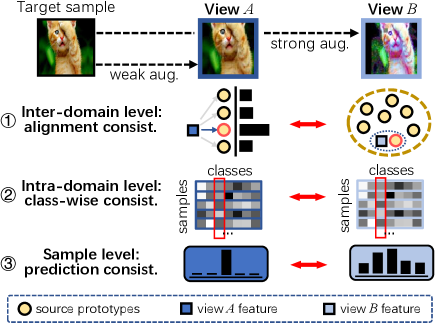
Although Li et al. (2021a) show that consistency regularization benefits SSDA, it has only been naively applied at the sample level, i.e., enforcing the prediction of an unlabeled target sample to be consistent with those of its different views (obtained via augmentations). However, in SSDA, it is also important to attend the inter-domain knowledge transfer to better leverage the source supervision and intra-domain representation learning for both compact and discriminative class clusters. Therefore, to fully utilize consistency regularization in SSDA, we propose a Multi-level Consistency Learning (MCL) framework, as shown in Fig. 1, which regularizes the model with (i) inter-domain level alignment consistency, (ii) intra-domain level class-wise assignment consistency, and (iii) sample level prediction consistency.
At the inter-domain level, we use consistency regularization to robustly and accurately align the source and target domain. We regularize the consistency between one view (weakly augmented target samples) to source mapping and another view (strongly augmented target samples) to source mapping. Specifically, we first solve the optimal transport mapping between one view of the target samples and the source prototypes, and leverage the solved mapping to cluster another view to the source prototypes. At the intra-domain level, we propose a novel class-wise contrastive clustering loss function to help the network learn both discriminative and compact feature representations in the target domain. This is implemented by computing the class-wise cross-correlation between the predictions from two views (target samples) in a mini-batch, and increasing the correlation of two views in the same class while reducing those from different classes. At the sample level, we follow standard practice and enforce the predictions of the weakly-augmented and the strongly-augmented views to be consistent. In this way, the sample-level information can be fully probed to learn better feature representations for each single unlabeled target sample. With our multi-level consistency learning framework, the model is encouraged to capture complementary and comprehensive information at different levels, thereby learning more well-aligned and discriminative target features.
In summary, our work has the following contributions: (1) We propose a novel Multi-level Consistency Learning (MCL) framework for SSDA tasks. Our framework benefits SSDA by fully utilizing the potential of consistency regularization at three levels: the inter-domain level, the intra-domain level, and the sample level. (2) Our inter-domain level consistency learning method consists of a novel mapping and clustering strategy, and a novel prototype-based optimal transport method, which yields more robust and accurate domain alignment. (3) Our intra-domain level consistency learning method consists of a novel class-wise contrastive clustering loss, which helps the network learn more compact intra-class and discriminative inter-class target features. (4) Extensive experiments on SSDA benchmarks demonstrate that our MCL framework achieves a new state-of-the-art result.
2 Related Work
Semi-supervised Domain Adaptation (SSDA)
Unlike UDA, SSDA assumes that there exist several labeled samples in the target domain, e.g. 3 shots per class. Many works have recently been proposed to tackle the SSDA problem Saito et al. (2019); Yang et al. (2021); Qin et al. (2021); Li et al. (2021b); Kim and Kim (2020); Li et al. (2021a); Jiang et al. (2020); Yao et al. (2022); Singh (2021). Saito et al. (2019) first proposes to solve the SSDA problem by min-maximizing the entropy of target unlabeled data. Jiang et al. (2020) train the network with virtual adversarial perturbations so that the network can generate robust features. Yang et al. (2021) decompose SSDA into an inter-domain UDA subtask and an intra-domain SSL subtask, and utilize co-training to make the two networks teach each other and learn complementary information. Qin et al. (2021) use two classifiers to learn scattered source features and compact target features, thereby enclosing target features by the expanded boundary of source features. Li et al. (2021a) propose to reduce the intra-domain gap by gradually clustering similar target samples together while pushing dissimilar samples away. In this work, instead of focusing on either inter-domain level or intra-domain level, we address both of them simultaneously so that the learning of both levels will benefit each other to learn more representative target features.
Consistency Regularization
Consistency regularization is a widely used technique in semi-supervised learning Sohn et al. (2020) and self-supervised learning Chen et al. (2020). In semi-supervised learning Sohn et al. (2020), enforcing the consistency among different augmentations of unlabeled samples can effectively boost the model performance. Recent works Chen et al. (2020) have shown that the consistency regularization objective can guide the model to learn meaningful representations in an unsupervised manner without any annotations, which inspires its application in label-scarce learning scenarios, e.g. domain adaptation, semi-supervised learning. Recently, some works have demonstrated that consistency regularization can also be utilized in domain adaptation tasks French et al. (2018). Although our work is also built upon consistency regularization, rather than regularizing the sample-wise predictions only, we additionally regularize the consistency at both inter-domain and intra-domain levels.
3 Methodology
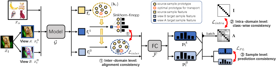
In this section, we first present the preliminaries including the definition of SSDA and associated notations, and then introduce the proposed Multi-level Consistency Learning (MCL) framework in detail. An outline of our MCL framework is illustrated in Fig. 2.
3.1 Preliminaries
In the semi-supervised domain adaptation (SSDA) problem, the source domain is fully labeled, and the target domain contains a few labels for partial samples , so , where is the unlabeled target sample set. SSDA methods aim to learn a classifier with high accuracy on the target domain using the rich data-label pairs and few ones . We assume that (i) the source and target domains share the same label space of classes; (ii) there are only a few labels for each class in the target domain, e.g. one label (1-shot) or three labels (3-shot).
SSDA model usually consists of two components, a feature extractor and a classifier , parameterized by and , respectively. Following Sohn et al. (2020), we first generate two views for each target sample , denoted as and , through the weak (view ) and strong (view ) augmentation, respectively. The two views are then fed into to obtain their feature representations , which finally go through to get the probabilistic prediction . This process can be formulated as:
| (1) |
where is the softmax function. Similarly, in the source branch, each source sample is fed into the same feature extractor to generate , and then into the classifier to obtain the prediction .
To train the model, each sample-label pair (from either the source or target domain) can be used to minimize a standard cross-entropy (CE) classification loss as follows:
| (2) |
where is the prediction of sample through and . As detailed below, to fully utilize the unlabeled target data , our MCL framework regularizes the consistencies in SSDA at three levels.
3.2 Inter-domain Alignment Consistency
At the inter-domain level, we propose a novel consistency regularization method to robustly and accurately align samples from the target domain to those of the source domain, so that the knowledge in the source domain can be better transferred into the target domain. To obtain such a high-quality alignment, we compute the mapping plan from two views of the target sample to the source sample, and leverage the consistency between the two mappings to guide the learning process. Specifically, in each iteration, we first compute the mapping from the view of a target sample to a source sample , according to which the representations of its view , and are clustered closer. Accordingly, our method alternates the following two steps throughout the training:
Step 1. View-A to Source Mapping.
We formulate the domain alignment as an optimal transport problem Courty et al. (2016), which aims to find the optimal sample-level coupling plan between source samples and view- target samples by minimizing the total transport cost:
| (3) | ||||
| (4) |
where denotes the transport plan between the th and th sample in the source and target domain, respectively, denotes the Frobenius inner product, is a -dimensional vector of 1’s, and are the empirical distributions of source and target samples, respectively, which are usually set as uniform distributions. is the cost function matrix to indicate the transport cost between each source-target sample pair, with each element in the matrix is inversely proportional to the cosine distance between the -th source feature and the -th view- target feature , computed as:
| (5) |
where more similar a feature vector pair is, a smaller transport cost can be obtained. With the cost matrix, computed, the total transport cost can be minimized to obtain the optimal coupling plan , of which each element indicates a correspondence score for alignment.
Step 2. View-B to Source Clustering.
With the guidance of optimal coupling , the feature representation of each strongly-augmented view- sample can be clustered toward the source prototype. In this way, the learned view- features can have a consistent mapping plan with the weakly-augmented view . Hence the objective of the inter-domain alignment consistency learning is to minimize the loss function as below:
| (6) | ||||
| (7) | ||||
| (8) |
so that can generate well-aligned view- features that are close to the corresponding source sample feature.
Prototype-based OT.
To further improve the accuracy and robustness, we propose to replace the source samples used in our OT method with source prototypes. Our source prototypes bring two benefits: (i) their features are more representative; (ii) they always cover all classes and avoid the misalignment error caused by missing classes in a mini-batch of source samples. To this end, for each class , we compute its prototype by averaging the feature representations of all source samples in and substitute all with in Eq. 3 and 5. In Step 2 of our method, after the update of , each in is updated with the batch mean and a momentum after each iteration:
| (9) |
Thus, we alternate between these two steps during training: (i) with fixed neural network parameters, solve the optimal coupling for view (Eq. 7), and (ii) with the optimal coupling fixed, optimize the alignment loss for view (Eq. 6).
3.3 Intra-domain Class-wise Consistency
To facilitate representation learning in the target domain, we incorporate consistency regularization into the intra-domain level. Specifically, we aim to learn both compact and discriminative class-wise clusters in the target domain, i.e., the clusters of the same class from two views should be grouped, while those of different classes should be pushed away from each other. Existing unsupervised contrastive learning methods focus on sample-level representation learning, which still hardly learn highly discriminative clusters for each class Khosla et al. (2020).
Instead of the sample-wise contrastive learning, we propose a novel class-wise contrastive clustering loss function, by modeling the cluster of each class as all samples’ classification confidence of this class in a batch, named as batch-wise class assignment (illustrated as the column bounded by a red rectangle in Fig .1). The class-wise contrastive clustering has two purposes, (i) keeping the consistency of two views for the same batch-wise class assignment (positive pairs), and (ii) enlarging the distance between the batch-wise assignment of different classes (negative pairs).
Formally, given a batch of target samples’ predictions , where is the mini-batch size and represents the confidence of classifying the th sample into the th class. With the cluster assumption that each feature of samples in the same class should form a high-density cluster, we regard each column of as the batch-wise assignment of one class. Although the columns of will dynamically change with the iteration of mini-batches during training, the class assignment in different views of the same image should be similar, while dissimilar to other images. Therefore, we compute the cross-correlation matrix between two views and to measure the class-wise similarity, formulated as:
| (10) |
where and are the batch prediction from view and , respectively. is an asymmetry matrix with each element measuring the similarity between ’s th column and ’s th column. The objective is to increase the correlation values between two views of the same class assignment (diagonal values) while reducing ones for different classes’ views (off-diagonal values), which yields the loss function of intra-domain prediction consistency learning:
| (11) |
where is a normalization function to keep the row summation as 1, e.g., similar to MCC Jin et al. (2020), divide the elements with its row summation, is an identity matrix, and denotes the summation of the absolute values of the matrix. Note that the loss function is the summation of two terms for respectively normalizing the rows and columns of the correlation matrix . Such two normalization operations can alleviate the influence of class imbalance in a batch, i.e., the values in the class assignment may be too large or small according to the number of samples that belong to this class. Intuitively, the normalized row of correlation values can be regarded as the scores of matching one class assignment with each column in the other view to be a positive pair. Thus the dual design helps bi-directional matching score computation, i.e., the th row in represents the matching scores from ’s th column to ’s each column, while the one in represents matching in the inverse direction.
Note that minimizing Eq. 11 has the following properties: i) The rows of and are encouraged to be sharper, which implements entropy minimization Grandvalet et al. (2005) in label-scarce scenarios. ii) For each sample, the prediction of view and are encouraged to become similar, which coincides with the consistency regularization Chen et al. (2020) that helps the network to learn better representations. iii) It avoids a trivial solution that predicts all samples as the same class: the diagonal values of the normalized cross-correlation matrix are enforced to be close to 1, which punishes the trivial solution by a large loss.
| R C | R P | P C | C S | S P | R S | P R | Mean | |||||||||
|---|---|---|---|---|---|---|---|---|---|---|---|---|---|---|---|---|
| Method | 1-shot | 3-shot | 1-shot | 3-shot | 1-shot | 3-shot | 1-shot | 3-shot | 1-shot | 3-shot | 1-shot | 3-shot | 1-shot | 3-shot | 1-shot | 3-shot |
| S+T | 55.6 | 60.0 | 60.6 | 62.2 | 56.8 | 59.4 | 50.8 | 55.0 | 56.0 | 59.5 | 46.3 | 50.1 | 71.8 | 73.9 | 56.9 | 60.0 |
| DANN | 58.2 | 59.8 | 61.4 | 62.8 | 56.3 | 59.6 | 52.8 | 55.4 | 57.4 | 59.9 | 52.2 | 54.9 | 70.3 | 72.2 | 58.4 | 60.7 |
| ENT | 65.2 | 71.0 | 65.9 | 69.2 | 65.4 | 71.1 | 54.6 | 60.0 | 59.7 | 62.1 | 52.1 | 61.1 | 75.0 | 78.6 | 62.6 | 67.6 |
| MME | 70.0 | 72.2 | 67.7 | 69.7 | 69.0 | 71.7 | 56.3 | 61.8 | 64.8 | 66.8 | 61.0 | 61.9 | 76.1 | 78.5 | 66.4 | 68.9 |
| UODA | 72.7 | 75.4 | 70.3 | 71.5 | 69.8 | 73.2 | 60.5 | 64.1 | 66.4 | 69.4 | 62.7 | 64.2 | 77.3 | 80.8 | 68.5 | 71.2 |
| MetaMME | - | 73.5 | - | 70.3 | - | 72.8 | - | 62.8 | - | 68.0 | - | 63.8 | - | 79.2 | - | 70.1 |
| BiAT | 73.0 | 74.9 | 68.0 | 68.8 | 71.6 | 74.6 | 57.9 | 61.5 | 63.9 | 67.5 | 58.5 | 62.1 | 77.0 | 78.6 | 67.1 | 69.7 |
| APE | 70.4 | 76.6 | 70.8 | 72.1 | 72.9 | 76.7 | 56.7 | 63.1 | 64.5 | 66.1 | 63.0 | 67.8 | 76.6 | 79.4 | 67.6 | 71.7 |
| ATDOC | 74.9 | 76.9 | 71.3 | 72.5 | 72.8 | 74.2 | 65.6 | 66.7 | 68.7 | 70.8 | 65.2 | 64.6 | 81.2 | 81.2 | 71.4 | 72.4 |
| STar | 74.1 | 77.1 | 71.3 | 73.2 | 71.0 | 75.8 | 63.5 | 67.8 | 66.1 | 69.2 | 64.1 | 67.9 | 80.0 | 81.2 | 70.0 | 73.2 |
| CDAC | 77.4 | 79.6 | 74.2 | 75.1 | 75.5 | 79.3 | 67.6 | 69.9 | 71.0 | 73.4 | 69.2 | 72.5 | 80.4 | 81.9 | 73.6 | 76.0 |
| DECOTA | 79.1 | 80.4 | 74.9 | 75.2 | 76.9 | 78.7 | 65.1 | 68.6 | 72.0 | 72.7 | 69.7 | 71.9 | 79.6 | 81.5 | 73.9 | 75.6 |
| MCL | 77.4 | 79.4 | 74.6 | 76.3 | 75.5 | 78.8 | 66.4 | 70.9 | 74.0 | 74.7 | 70.7 | 72.3 | 82.0 | 83.3 | 74.4 | 76.5 |
| Method | R C | R P | R A | P R | P C | P A | A P | A C | A R | C R | C A | C P | Mean |
|---|---|---|---|---|---|---|---|---|---|---|---|---|---|
| One-shot | |||||||||||||
| S+T | 52.1 | 78.6 | 66.2 | 74.4 | 48.3 | 57.2 | 69.8 | 50.9 | 73.8 | 70.0 | 56.3 | 68.1 | 63.8 |
| DANN | 53.1 | 74.8 | 64.5 | 68.4 | 51.9 | 55.7 | 67.9 | 52.3 | 73.9 | 69.2 | 54.1 | 66.8 | 62.7 |
| ENT | 53.6 | 81.9 | 70.4 | 79.9 | 51.9 | 63.0 | 75.0 | 52.9 | 76.7 | 73.2 | 63.2 | 73.6 | 67.9 |
| MME | 61.9 | 82.8 | 71.2 | 79.2 | 57.4 | 64.7 | 75.5 | 59.6 | 77.8 | 74.8 | 65.7 | 74.5 | 70.4 |
| APE | 60.7 | 81.6 | 72.5 | 78.6 | 58.3 | 63.6 | 76.1 | 53.9 | 75.2 | 72.3 | 63.6 | 69.8 | 68.9 |
| CDAC | 61.9 | 83.1 | 72.7 | 80.0 | 59.3 | 64.6 | 75.9 | 61.2 | 78.5 | 75.3 | 64.5 | 75.1 | 71.0 |
| DECOTA | 56.0 | 79.4 | 71.3 | 76.9 | 48.8 | 60.0 | 68.5 | 42.1 | 72.6 | 70.7 | 60.3 | 70.4 | 64.8 |
| MCL | 67.0 | 85.5 | 73.8 | 81.3 | 61.1 | 68.0 | 79.5 | 64.4 | 81.2 | 78.4 | 68.5 | 79.3 | 74.0 |
| Three-shot | |||||||||||||
| S+T | 55.7 | 80.8 | 67.8 | 73.1 | 53.8 | 63.5 | 73.1 | 54.0 | 74.2 | 68.3 | 57.6 | 72.3 | 66.2 |
| DANN | 57.3 | 75.5 | 65.2 | 69.2 | 51.8 | 56.6 | 68.3 | 54.7 | 73.8 | 67.1 | 55.1 | 67.5 | 63.5 |
| ENT | 62.6 | 85.7 | 70.2 | 79.9 | 60.5 | 63.9 | 79.5 | 61.3 | 79.1 | 76.4 | 64.7 | 79.1 | 71.9 |
| MME | 64.6 | 85.5 | 71.3 | 80.1 | 64.6 | 65.5 | 79.0 | 63.6 | 79.7 | 76.6 | 67.2 | 79.3 | 73.1 |
| APE | 66.4 | 86.2 | 73.4 | 82.0 | 65.2 | 66.1 | 81.1 | 63.9 | 80.2 | 76.8 | 66.6 | 79.9 | 74.0 |
| CDAC | 67.8 | 85.6 | 72.2 | 81.9 | 67.0 | 67.5 | 80.3 | 65.9 | 80.6 | 80.2 | 67.4 | 81.4 | 74.2 |
| DECOTA | 70.4 | 87.7 | 74.0 | 82.1 | 68.0 | 69.9 | 81.8 | 64.0 | 80.5 | 79.0 | 68.0 | 83.2 | 75.7 |
| MCL | 70.1 | 88.1 | 75.3 | 83.0 | 68.0 | 69.9 | 83.9 | 67.5 | 82.4 | 81.6 | 71.4 | 84.3 | 77.1 |
3.4 Sample Prediction Consistency
Similar to Li et al. (2021a), we regularize the consistency at the sample level via pseudo labeling: the prediction of view of a target sample is set as the pseudo label of view of the target sample. Specifically, for each sample , we compute the cross-entropy loss as:
| (12) |
where and are the th elements in the prediction of from view and view , respectively, is the indication function, and is the threshold of confidence score.
3.5 Overall Objective Function
Therefore, the overall objective can be formulated as:
| (13) |
where and are the hyper-paramters to balance and , respectively.
| Method | 1-shot | 3-shot |
|---|---|---|
| S+T | 60.2 | 64.6 |
| ENT | 63.6 | 72.7 |
| MME | 68.7 | 70.9 |
| APE | 78.9 | 81.0 |
| CDAC | 69.9 | 80.6 |
| DECOTA | 64.9 | 80.7 |
| MCL | 86.3 | 87.3 |
4 Experiments
4.1 Experiment Setups
Datasets.
We evaluate our proposed MCL on several popular benchmark datasets, including VisDA2017 Peng et al. (2017), DomainNet Peng et al. (2019), and Office-Home Venkateswara et al. (2017). DomainNet was first introduced as the multi-source domain adaptation benchmark, and it consists of 6 domains with 345 categories. Following recent works Saito et al. (2019); Li et al. (2021a), the Real, Clipart, Painting, Sketch domains with 126 categories are selected for evaluations. VisDA2017 is a popular synthetic-to-real domain adaptation benchmark, which consists of 150k synthetic and 55k real images from 12 categories. Office-Home is a popular domain adaptation benchmark, which consists of 4 domains (Real, Clipart, Product, Art) and 65 categories. Following most recent works Yang et al. (2021); Li et al. (2021a), we conduct 1-shot and 3-shot experiments on all datasets. Note that we follow most UDA works Long et al. (2013) to report the Mean Class-wise Accuracy (MCA) as the evaluation metric for VisDA2017 and overall accuracy for DomainNet and Office-Home datasets.
Implementation details.
Similar to Saito et al. (2019); Li et al. (2021a), we use a ResNet34 as the backbone for most experiments. The backbone is pre-trained on Imagenet Deng et al. (2009). The batch size, optimizer, feature size, learning rate, etc. are set as same as in Saito et al. (2019). Similar to Li et al. (2021a), the threshold (Eq. 12) is set as 0.95, and we use the softmax temperature to control the sharpness of the prediction for the thresholding operation (1 for Domainnet, 1.25 for Office-Home and VisDA). The loss weight balancing hyperparameters is set as 1, and is set to 1 for DomainNet, 0.2 for Office-Home , and 0.1 for VisDA. We use RandomFlip and RandomCrop as the augmentation methods for view and RandAugment Cubuk et al. (2020) for view . For the OT solver, we introduce soft regularizations to the OT objective to make it a convex optimization problem that can be efficiently solved by Sinkhorn-Knopp iterations Fatras et al. (2021). Moreover, the momentum used to update source prototypes is set to 0.9. We use Pytorch and POT111https://pythonot.github.io to implement our MCL framework.
4.2 Comparative Results
We compare our MCL framework with i) two baseline methods S+T and ENT Grandvalet et al. (2005); and ii) several existing methods, including DANN Ganin et al. (2016), MME Saito et al. (2019), UODA Qin et al. (2021), BiAT Jiang et al. (2020), MetaMME Li and Hospedales (2020), APE Kim and Kim (2020), ATDOC Liang et al. (2021), STar Singh et al. (2021), CDAC Li et al. (2021a), and DECOTA Yang et al. (2021). Between the two baselines, “S+T” uses only source samples and labeled target samples in the training; “ENT” uses entropy minimization for unlabeled samples Grandvalet et al. (2005). Note that all methods are implemented on a ResNet34 backbone for a fair comparison.
Domainnet.
Results on the DomainNet dataset are shown in Tab. 1. To our knowledge, the proposed MCL achieves a new state-of-the-art (SOTA) performance, 74.4% and 76.5% mean accuracy over 7 adaptation scenarios, under the 1-shot and 3-shot setting, respectively.
Office-Home.
Results on the Office-Home dataset further validate the effectiveness of MCL. As shown in Tab. 2, MCL consistently outperforms other methods on both the 1-shot and 3-shot settings, and on all 12 adaptation scenarios. The mean accuracy of MCL reaches 74.0% and 77.1%, which outperform the SOTA performance by around 3% and 1.4%, under the 1-shot and 3-shot settings, respectively.
VisDA.
As shown in Tab. 3, MCL outperforms all existing SOTA methods in both 1-shot and 3-shot settings. Our MCL achieves 86.3% MCA under the 1-shot setting, and 87.3% for the 3-shot setting, significantly surpassing existing methods.
| A R | C P | ||||||
|---|---|---|---|---|---|---|---|
| 1-shot | 3-shot | 1-shot | 3-shot | ||||
| () | 73.8 | 74.2 | 68.1 | 72.3 | |||
| () | ✓ | 75.8 | 77.7 | 72.5 | 78.6 | ||
| () | ✓ | 79.3 | 81.1 | 76.0 | 79.4 | ||
| () | ✓ | 75.5 | 77.2 | 72.8 | 79.1 | ||
| () | ✓ | ✓ | 79.7 | 81.1 | 78.2 | 81.6 | |
| () | ✓ | ✓ | 75.9 | 78.2 | 73.9 | 82.0 | |
| () | ✓ | ✓ | 79.3 | 81.5 | 78.4 | 82.9 | |
| () | ✓ | ✓ | ✓ | 81.2 | 82.4 | 79.3 | 84.3 |
| OT | CC | Accuracy | |||
|---|---|---|---|---|---|
| Standard | Proto. | Sample | Class | C S | P R |
| ✓ | ✓ | 66.5 | 80.0 | ||
| ✓ | ✓ | 67.4 | 81.2 | ||
| ✓ | ✓ | 69.2 | 81.9 | ||
| ✓ | ✓ | 70.9 | 83.3 | ||
4.3 Analysis
Ablation studies.
We conduct ablation studies on the Office-Home of A R and C P, and under both 1-shot and 3-shot settings, as shown in Tab. 4. Row (b)(c)(d) show that each component can yeild significant improvement. Row (e)(f)(g) show that each combination can still improve the performance, which indicates the versatility of the proposed modules. The best performance is achieved with all components activated.
Prototype-based OT.
In the proposed MCL, prototype-based OT is adopted to compute the mapping plan between target samples and source prototypes, which generates more representative source features for transport to learn robust inter-domain alignment. In comparison, we also implement sample-wise OT on the DomainNet dataset under the 3-shot setting, with other hyper-parameters the same as MCL. Evaluation results on two adaptation scenarios are listed in Tab. 5, sample-wise OT (“Standard”) results in a drop of 3.5% (C S) and 2.1% (P R), which verify our claim.
Class-wise contrastive clustering.
In the design of class-wise contrastive clustering loss, an alternative is to compute the sample-wise correlation matrix instead, where is the batch size. We claim that such a sample-wise operation is inferior, and experimental results on the DomainNet dataset under the 3-shot setting support our argument, as listed in Tab. 5. One potential reason might be that the class-wise inner product focuses on clustering each class for higher compactness, whereas the sample-wise one pays more attention to the correlation between individual samples, which is less effective when labels are scarce and compact representations are difficult to generate.
5 Conclusion
In this paper, we presented a novel Multi-level Consistency Learning (MCL) framework for the SSDA problem. MCL consists of three levels of consistency regularization, (i) inter-domain alignment consistency for learning robust inter-domain alignment via a prototype-based optimal transport method, (ii) intra-domain class-wise consistency for learning both compact and discriminative class clusters, and (iii) sample-level prediction consistency to better leverage instance-wise information. Our MCL approach well leverages information at multiple levels, with extensive experiments and ablation studies solidly proving its superiority.
Acknowledgments
The work was supported in part by Chinese Key-Area Research and Development program of Guangdong Province (2020B0101350001), by the Basic Research Project No. HZQB-KCZYZ-2021067 of Hetao Shenzhen-HK S&T Cooperation Zone, by National Key R&D Program of China with grant No. 2018YFB1800800, by Shenzhen Outstanding Talents Training Fund 202002, by Guangdong Research Projects No. 2017ZT07X152 and No. 2019CX01X104, by the National Natural Science Foundation of China under Grant No.61976250 and No.U1811463, by the Guangzhou Science and technology project under Grant No.202102020633 and by Shenzhen Research Institute of Big Data. Thanks to the ITSO in CUHKSZ for their High-Performance Computing Services.
References
- Chen et al. [2020] Ting Chen, Simon Kornblith, Mohammad Norouzi, and Geoffrey Hinton. A simple framework for contrastive learning of visual representations. In ICML, 2020.
- Courty et al. [2016] Nicolas Courty, Rémi Flamary, Devis Tuia, and Alain Rakotomamonjy. Optimal transport for domain adaptation. TPAMI, 2016.
- Cubuk et al. [2020] Ekin D Cubuk, Barret Zoph, Jonathon Shlens, and Quoc V Le. Randaugment: Practical automated data augmentation with a reduced search space. In CVPR Workshops, 2020.
- Deng et al. [2009] Jia Deng, Wei Dong, Richard Socher, Li-Jia Li, Kai Li, and Li Fei-Fei. Imagenet: A large-scale hierarchical image database. In CVPR, 2009.
- Fatras et al. [2021] Kilian Fatras, Thibault Séjourné, Rémi Flamary, and Nicolas Courty. Unbalanced minibatch optimal transport; applications to domain adaptation. In ICML, 2021.
- French et al. [2018] Geoffrey French, Michal Mackiewicz, and Mark Fisher. Self-ensembling for visual domain adaptation. In ICLR, 2018.
- Ganin et al. [2016] Yaroslav Ganin, Evgeniya Ustinova, Hana Ajakan, Pascal Germain, Hugo Larochelle, François Laviolette, Mario Marchand, and Victor Lempitsky. Domain-adversarial training of neural networks. JMLR, 2016.
- Grandvalet et al. [2005] Yves Grandvalet, Yoshua Bengio, et al. Semi-supervised learning by entropy minimization. In CAP, 2005.
- Jiang et al. [2020] Pin Jiang, Aming Wu, Yahong Han, Yunfeng Shao, Meiyu Qi, and Bingshuai Li. Bidirectional adversarial training for semi-supervised domain adaptation. In IJCAI, 2020.
- Jin et al. [2020] Ying Jin, Ximei Wang, Mingsheng Long, and Jianmin Wang. Minimum class confusion for versatile domain adaptation. In ECCV, 2020.
- Khosla et al. [2020] Prannay Khosla, Piotr Teterwak, Chen Wang, Aaron Sarna, Yonglong Tian, Phillip Isola, Aaron Maschinot, Ce Liu, and Dilip Krishnan. Supervised contrastive learning. In NeurIPS, 2020.
- Kim and Kim [2020] Taekyung Kim and Changick Kim. Attract, perturb, and explore: Learning a feature alignment network for semi-supervised domain adaptation. In ECCV, 2020.
- Li and Hospedales [2020] Da Li and Timothy Hospedales. Online meta-learning for multi-source and semi-supervised domain adaptation. In ECCV, 2020.
- Li et al. [2021a] Jichang Li, Guanbin Li, Yemin Shi, and Yizhou Yu. Cross-domain adaptive clustering for semi-supervised domain adaptation. In CVPR, 2021.
- Li et al. [2021b] Kai Li, Chang Liu, Handong Zhao, Yulun Zhang, and Yun Fu. Ecacl: A holistic framework for semi-supervised domain adaptation. In ICCV, 2021.
- Liang et al. [2021] Jian Liang, Dapeng Hu, and Jiashi Feng. Domain adaptation with auxiliary target domain-oriented classifier. In CVPR, 2021.
- Long et al. [2013] Mingsheng Long, Jianmin Wang, Guiguang Ding, Jiaguang Sun, and Philip S Yu. Transfer feature learning with joint distribution adaptation. In ICCV, 2013.
- Peng et al. [2017] Xingchao Peng, Ben Usman, Neela Kaushik, Judy Hoffman, Dequan Wang, and Kate Saenko. Visda: The visual domain adaptation challenge. arXiv preprint arXiv:1710.06924, 2017.
- Peng et al. [2019] Xingchao Peng, Qinxun Bai, Xide Xia, Zijun Huang, Kate Saenko, and Bo Wang. Moment matching for multi-source domain adaptation. In ICCV, 2019.
- Qin et al. [2021] Can Qin, Lichen Wang, Qianqian Ma, Yu Yin, Huan Wang, and Yun Fu. Contradictory structure learning for semi-supervised domain adaptation. In SDM, 2021.
- Saito et al. [2019] Kuniaki Saito, Donghyun Kim, Stan Sclaroff, Trevor Darrell, and Kate Saenko. Semi-supervised domain adaptation via minimax entropy. In ICCV, 2019.
- Singh et al. [2021] Anurag Singh, Naren Doraiswamy, Sawa Takamuku, Megh Bhalerao, Titir Dutta, Soma Biswas, Aditya Chepuri, Balasubramanian Vengatesan, and Naotake Natori. Improving semi-supervised domain adaptation using effective target selection and semantics. In CVPRW, 2021.
- Singh [2021] Ankit Singh. Clda: Contrastive learning for semi-supervised domain adaptation. In NeurlPS, 2021.
- Sohn et al. [2020] Kihyuk Sohn, David Berthelot, Chun-Liang Li, Zizhao Zhang, Nicholas Carlini, Ekin D Cubuk, Alex Kurakin, Han Zhang, and Colin Raffel. Fixmatch: Simplifying semi-supervised learning with consistency and confidence. In NeurIPS, 2020.
- Venkateswara et al. [2017] Hemanth Venkateswara, Jose Eusebio, Shayok Chakraborty, and Sethuraman Panchanathan. Deep hashing network for unsupervised domain adaptation. In CVPR, 2017.
- Xie et al. [2019] Qizhe Xie, Zihang Dai, Eduard Hovy, Minh-Thang Luong, and Quoc V Le. Unsupervised data augmentation for consistency training. In NeurIPS, 2019.
- Yang et al. [2021] Luyu Yang, Yan Wang, Mingfei Gao, Abhinav Shrivastava, Kilian Q. Weinberger, Wei-Lun Chao, and Ser-Nam Lim. Deep co-training with task decomposition for semi-supervised domain adaptation. In ICCV, 2021.
- Yao et al. [2022] Huifeng Yao, Xiaowei Hu, and Xiaomeng Li. Enhancing pseudo label quality for semi-superviseddomain-generalized medical image segmentation. arXiv preprint arXiv:2201.08657, 2022.