Multi-object Monocular SLAM for Dynamic Environments
Abstract
In this paper, we tackle the problem of multibody SLAM from a monocular camera. The term multibody, implies that we track the motion of the camera, as well as that of other dynamic participants in the scene. The quintessential challenge in dynamic scenes is unobservability: it is not possible to unambiguously triangulate a moving object from a moving monocular camera. Existing approaches solve restricted variants of the problem, but the solutions suffer relative scale ambiguity (i.e., a family of infinitely many solutions exist for each pair of motions in the scene). We solve this rather intractable problem by leveraging single-view metrology, advances in deep learning, and category-level shape estimation. We propose a multi pose-graph optimization formulation, to resolve the relative and absolute scale factor ambiguities involved. This optimization helps us reduce the average error in trajectories of multiple bodies over real-world datasets, such as KITTI [1]. To the best of our knowledge, our method is the first practical monocular multi-body SLAM system to perform dynamic multi-object and ego localization in a unified framework in metric scale.
I Introduction
Monocular SLAM research has significantly matured over the last few decades, resulting in very stable off-the-shelf solutions [2, 3, 4]. However, dynamic scenes still pose unique challenges for even the best such solutions. In this work, we tackle a more general version of the monocular SLAM problem in dynamic environments: multi-body visual SLAM. While monocular SLAM methods traditionally track the ego-motion of a camera and discard dynamic objects in the scene, multi-body SLAM deals with the explicit pose estimation of multiple dynamic objects (dynamic bodies), which finds important applications in the context of autonomous driving.
Despite being an extremely useful problem, multibody visual SLAM has not received comparable attention to its uni-body counterpart (i.e., SLAM using stationary landmarks). This can primarily be attributed to the ill-posedness of monocular multibody Structure-from-Motion [5]. While the scale factor ambiguity of monocular SLAM is well-known [6, 2, 3, 4], the lesser-known-yet-well-studied relative scale problem persists with multibody monocular SLAM [7, 8, 5, 9, 10, 11, 12]. In a nutshell, relative-scale ambiguity refers to the phenomenon where the estimated trajectory is ambiguous, and is recovered as a one-parameter family of trajectories relative to the ego-camera. Each dynamic body has a different, uncorrelated relative-scale, which renders the problem unobservable [5] and degeneracy-laden [7, 9, 12]. This incites us to explore the usage of static feature correspondences in the environment for ego and dynamic vehicle motion estimation in metric scale111We use the term metric scale to denote a coordinate frame in which all distances are expressed in units of metres..
We propose a multi pose-graph optimization framework for dynamic objects in a scene, and demonstrate its ability to solve for multiple object motions including ego vehicle unambiguously, in a unified global frame in metric scale. To the best of our knowledge, this is the first monocular multibody SLAM to represent moving obstacle trajectories in a unified global metric frame, on long real-world dynamic trajectories. The quantitative results presented in Sec. VI demonstrate the efficacy of the proposed formulation.
In the remainder of this paper, we elaborate upon the following key contributions:
-
1.
Leveraging single-view metrology for scale-unambiguous static feature correspondence estimation
-
2.
A multi pose-graph formulation that recovers a metric scale solution to the multibody SLAM problem.
-
3.
Practicality: Evaluation of our approach on challenging sequences from the KITTI driving dataset [1]
II Related Work
The earliest approaches to monocular multibody SLAM [13, 14, 9, 15, 16] were based on motion segmentation: segmenting multiple motions from a set of triangulated points. Extending epipolar geometry to multiple objects, multibody fundamental matrices were used in [9, 10, 11, 16].
Trajectory triangulation methods [17, 8], on the other hand, derive a set of constraints for trajectories of objects, and solve the multi-body SLAM problem under these constraints. Ozden et al. [5] extend the multi-body Structure-from-Motion framework [14] to cope with practical issues, such as a varying number of independently moving objects, track failure, etc. Another class of approaches applies model selection methods to segment independently moving objects in a scene, and then explicitly solve for relative scale solutions [10, 14, 13]. It is worth noting that the above approaches operate offline, and extending them for online operation is non-trivial.
Kundu et al. [7] proposed a fast, incremental multi-body SLAM system that leverages motion segmentation to assign feature tracks to dynamic bodies, and then independently for relative-scale for the segmented motions. Critical to their success is the underlying assumption of smooth camera motions. Later Namdev et al. [12] provided analytical solutions for a restricted set of vehicle motions, (linear, planar, and nonholonomic).
More recently, Ranftl et al. [18] presented a dense monocular depth estimation pipeline targeted at dynamic scenes, and resolve relative scale ambiguity. CubeSLAM [19] proposes an object SLAM framework for road scenes. However, it only estimates a per-frame relative pose for each object, and does not unify it to construct a trajectory (to avoid relative-scale-ambiguity).
With the advent of deep learning, improvements to object detection [20, 21, 22, 23] and motion segmentation have resulted in such methods directly being employed in multi-body SLAM. Reddy et al. [24] and Li et al. [25] present approaches to multi-body SLAM using a stereo camera. In this case, however, the problem is observable, while we handle the harder, unobservable case of monocular cameras.
III Overview of the Proposed Pipeline
With sequence of traffic scene frames as input, our formulation estimates:
-
1.
Ego-motion obtained as the camera motion in metres in a static global system for each input frame with an SE(3) formulation.
-
2.
Trajectory estimates to each object in the traffic scene being captured by the camera in metres in static global frame for each input frame with an SE(3) formulation.
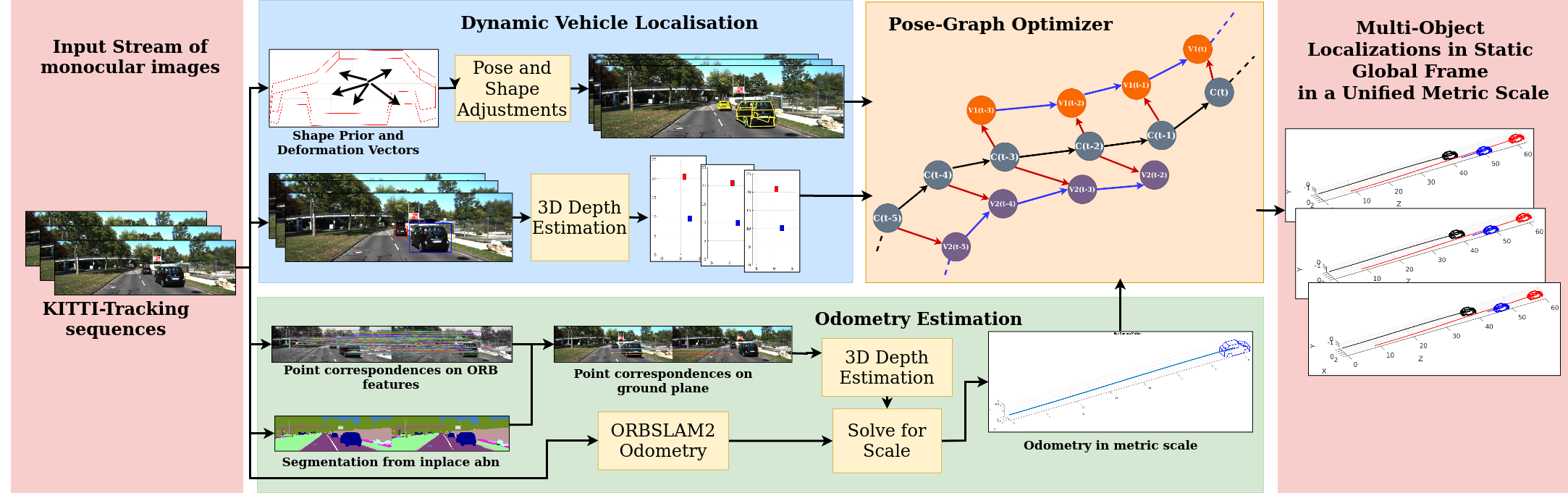
We obtain the above estimates with a pipeline summarized in the following manner:
-
1.
We take a stream of monocular images as input to our pipeline.
-
2.
We exploit 3D depth estimation to ground plane points as a source of vehicle localizations in ego-camera frame as explained in Sec. IV-A.
-
3.
Alternatively, as explained in Sec. IV-C, we fit a base shape prior to each vehicle instance uniquely to obtain refined vehicle localizations in ego-camera frame.
- 4.
-
5.
Finally, our optimization formulation (cf. Sec. V) utilizes the above estimates to resolve cyclic-consistencies in the pose-graph.
-
6.
This provides us with accurate multi-body localizations in a static global frame and consistent metric scale.
IV Vehicle Localization and Odometry Estimation
IV-A Depth Estimation for Points on Ground Plane
We utilize the known camera intrinsic parameters , ground plane normal , 2D bounding boxes[27] and camera height in metric unit to estimate the depth of any point on the ground plane222Flat-earth assumption: For the scope of this paper, we assume that the autonomous vehicle is operating within a bounded geographic area of the size of a typical city, and that all roads in consideration are somewhat planar, i.e., no steep/graded roads on mountains.. Given the 2D homogeneous coordinates to the point in image space to be , we estimate the 3D depth to them using the following method as shown in Song et al.[28].
| (1) |
IV-B Odometry Estimations
The initializations to our odometry pipeline (cf. Fig. 2) come from the ORB trajectory[26] in a static-global frame but in an ambiguous ORB scale as opposed to our requirement of metric scale.
We scale the ego-motion from the ORB-SLAM2[26] input by minimizing the re-projection error of the ground point correspondences between each pair of consecutive frames. Given frames and , we have odometry initializations in 3D in ORB scale from ORB-SLAM2 as and respectively. We obtain the relative odometry between the two frames as follows333We use to denote matrix multiplication for the scope of this paper.:
| (2) |
We now obtain ORB features to match point correspondences between the two frames and and use state-of-the-art semantic segmentation network[20] to retrieve points and that lie on the ground plane. We obtain the corresponding points and in 3D, given the camera height, via Eqn. 1 as explained in Sec. IV-A. To reduce the noise incorporated by the above method, we only consider points within a threshold in depth of T = 12 metres from the camera. Further, we obtain the required scale-factor that scales odometry from Eqn. 2 via a minimization problem as shown in Eqn. 4, the objective function to which is elaborated as Eqn. 3:
| (3) |
| (4) |
Here, and represent the relative rotation matrix and translation vector respectively. After solving the above minimization problem, we finalize our scale factor as the mean of solutions obtained from the following:
| (5) |
IV-C Pose and Shape Adjustments Pipeline
We obtain object localizations by using a method inspired from Murthy et al.[29]. Our object representation follows from [30, 29, 31], based on a shape prior consisting of ordered keypoints which represent specific visually distinguishable features on objects which primarily consist of cars and minivans. For this work, we stick with the 36 keypoints structure from Ansari et al.[31]. We obtain the keypoint localizations in 2D image space using a CNN based on stacked hourglass architecture[32] and use the same model trained on over 2.4 million rendered images for Ansari et al.[31].
Borrowing the notations from Murthy et al.[29], we begin with a basis shape prior for the object used as a mean shape . Let basis vectors be and the corresponding deformation coefficients be . Assuming that a particular object instance has a rotation of and translation of with respect to the camera, its instance in the scene can be shown mathematically using the following shape prior model:
| (6) |
Here, and . Also, represents the basis shape prior and the resultant shape for the object instance is where each represents one of the k = 36 keypoints in 3D coordinate system from camera’s perspective. Now, Let the ordered collection of keypoint localizations in 2D image space be . Given that represents the function to project 3D coordinates onto 2D image space using the camera intrinsics , fairly accurate estimates for the pose parameters (R, tr) and the shape parameter () for the object instance can be obtained using the following objective function:
| (7) |
| (8) |
Minimizing the objective function (cf. Eqn 7) separately for pose parameters (R, tr) and shape parameters () provides us with an optimal fitting of the shape prior over the dynamic object. We obtain the object orientation as after pose parameter adjustments. The object’s 3D coordinates from the camera is obtained from the mean of wheel centres.
V Multi-Object Pose Graph Optimizer
V-A Pose-Graph Components
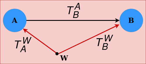
Fig. 3 illustrates a simple pose-graph structure containing two nodes A and B and a binary-edge between them. Using the terminologies from g2o[33], any node A in the pose graph is characterized by a pose called the estimate which defines its pose with respect to the static-global frame of reference W. Meanwhile, a binary-edge from A to B is represented with a relative pose called the measurement which defines the pose of node B from node A’s perspective. Mathematically, the constraint introduced by the binary-edge is given as:
| (9) |
Assuming relative correctness between each term in Eqn. 9, it results in an identity matrix irrepective of the order of transformation. Thus, Eqn. 9 reduces to:
| (10) |
Clearly, the order in which the transformations are applied do not change the consistency of the respective cycle in the pose-graph. Thus, Eqn. 10 can also be written as:
| (11) |
V-B Pose-Graph Formulation
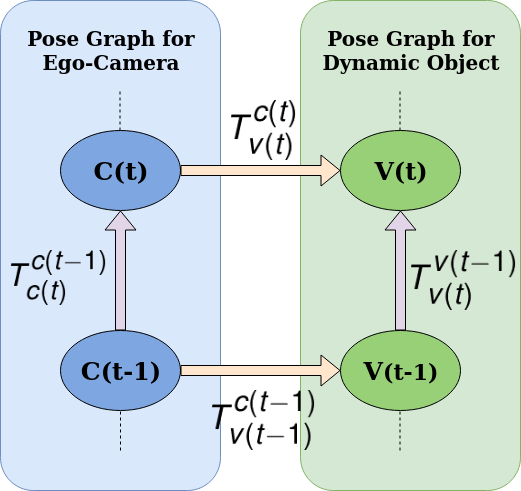
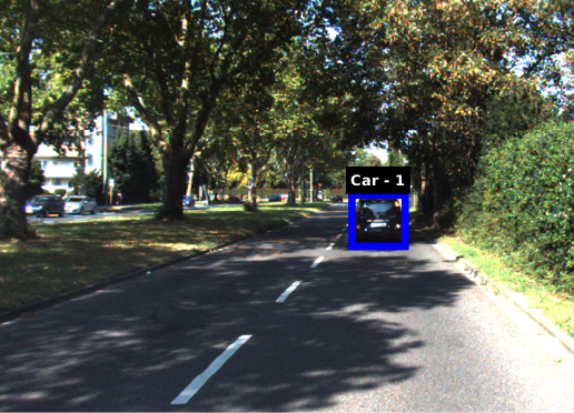
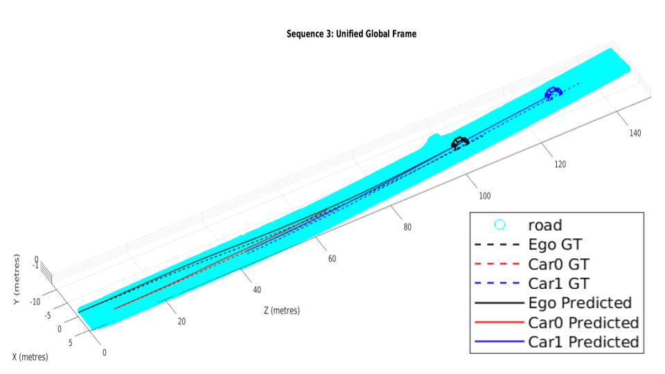
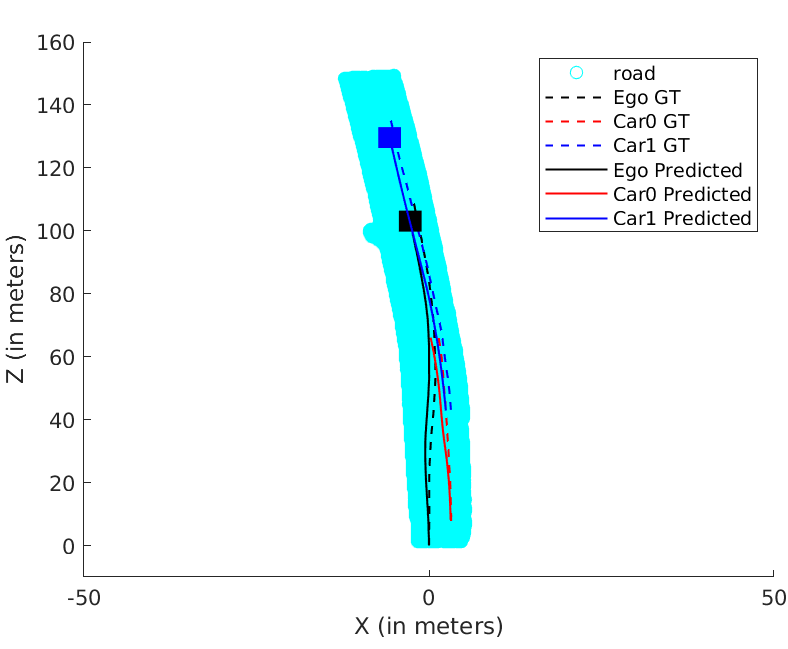
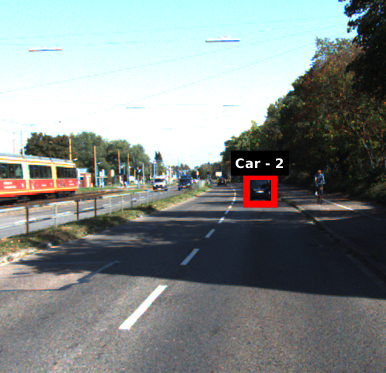
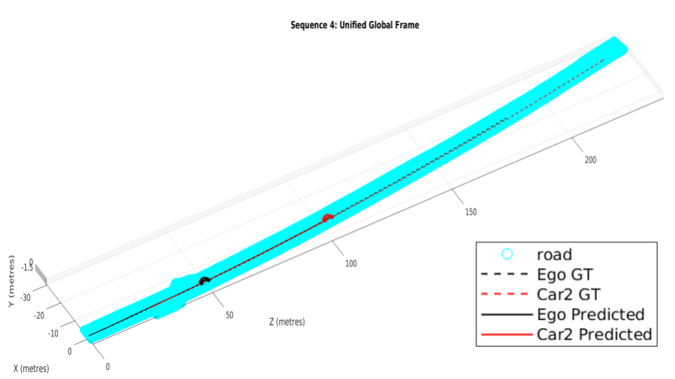
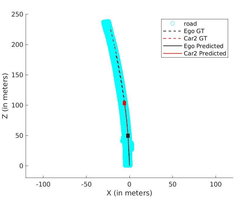
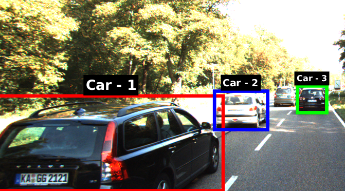
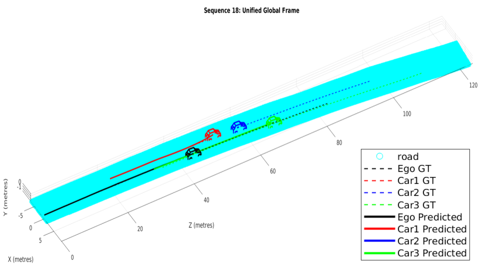
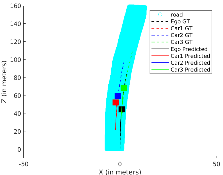
Fig. 4 illustrates the pose graph structure between every consecutive set of frames and containing four nodes and four edges between them. We obtain the estimates for camera nodes and (i.e., and ) and measurement for the camera-camera edge (i.e. ) from our odometry estimation (cf. Sec. IV-B). We use this odometry to register dynamic object localizations from pose-shape adjustment pipeline as explained in Sec. IV-C to provide for the estimates and to vehicle nodes and . We obtain measurement for the camera-vehicle edge (i.e., , ) from shape and pose adjustment (cf. Sec. IV-C). Moreover, we use depth estimation from ground plane using Song et al.[28] as explained in Sec. IV-A as a source of vehicle localization that is unique from the localizations obtained from Sec. IV-C. This registered with our odometry estimations provides for our vehicle-vehicle edge measurement i.e., . Now, from Eqn. 10, the cost function for the above binary-edges, , , and , can be defined mathematically as:
| (12) |
Cumulatively, the above cost functions for a single loop illustrated in Fig. 4 can be represented as:
| (13) |
On substituting Eqn. 12 in Eqn. 13, and on further simplification, we obtain the resultant function for cumulative cost which clearly defines the cyclic consistency within the loop defined by the four binary edges:
| (14) |
V-C Confidence Parameterization
In addition to the relative pose between the participating graph nodes, the parameterization for each edge also includes a positive semi-definite inverse covariance matrix or the information matrix where E represents an edge in the pose graph and N represents the dimension of the Lie group in which the poses are defined. In this work, all poses and transformations are defined in SE(3), hence we can take N = 6 for the information matrix corresponding to each edge E in the whole pose graph. We utilize this as a confidence parameterization for the sources of input-data into the pose-graph. To make the most out of this, we scale the information matrix for an edge by a scale factor to get the effective information matrix that is finally sent as a parameter:
| (15) |
We categorize all the edges in our pose-graph formulation into three types namely camera-camera, camera-vehicle, and vehicle-vehicle edges. Each type of edges corresponds to a unique source of data to provide for the corresponding constraint. This formulation coupled with the corresponding confidence parameter , enables us to scale the effects of the respective categories of edges appropriately. Given that odometry estimates are fairly reliable, we assign a relatively high constant scaling to its information matrix for our experiments on all sequences.
Given that we obtain dynamic vehicle localizations in camera frame from two different sources as explained in Sec. V-A, we make intelligent use of the confidence parameter , to scale the information matrix corresponding to the camera-vehicle and the vehicle-vehicle edges in our pose graph. It has been observed over a large number of vehicles that localizations obtained from Sec. IV-C performs better than the those obtained from Sec. IV-A for vehicles closer to the camera (up to about 45 metres). This can be attributed to the keypoint localizations being inaccurate for far away objects. However, estimates from Sec. IV-A are more accurate at depths far away from the camera (over 45 metres). Factors like visible features on vehicles do not affect these estimates.
VI Experiments and Results
VI-A Dataset
We test our procedure over a wide range of KITTI-Tracking training sequences[1], spanning over rural and urban scenarios with various number of dynamic objects in the scene. We perform localizations on objects primarily consisting of cars and mini-vans. Our localization pipeline provides accurate results over objects irrespective of the direction of motion and maneuvers undertaken by both the ego-car and the vehicles in the scene. The labels provided in the dataset are used as ground truth for getting the depth to the vehicle’s center from the camera. The corresponding ground truth for odometry comes from GPS/IMU data, which is compiled using the OXTS data provided for all the KITTI-Tracking training sequences.
VI-B Qualitative Results
VI-B1 Pose and Shape Adjustments
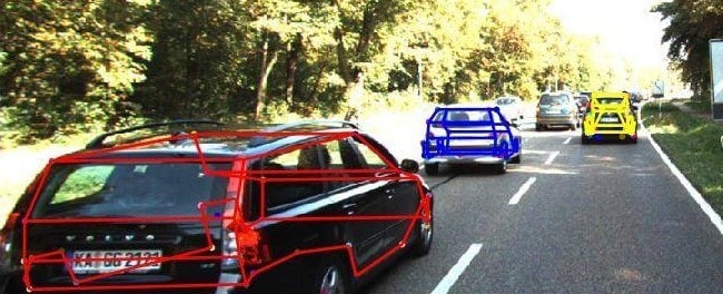
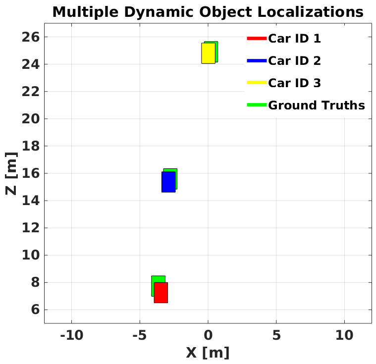
We obtain accurate localizations in ego-camera frame by fitting base shape priors to each non-occluded and non-truncated vehicle in the scene with respect to the ego-camera. While the pipeline is dependent on the keypoint localizations on these vehicles, factors like large depth from camera are bound to affect the accuracies with respect to ground truth. However, this approach ensures fairly accurate vehicle localizations for the pose-graph optimizer to apply its edge constraints. Fig. 6 illustrates wireframe fitting and subsequent mapping in ego-frame for a traffic scenario consisting of multiple vehicles.
VI-B2 Odometry Estimation
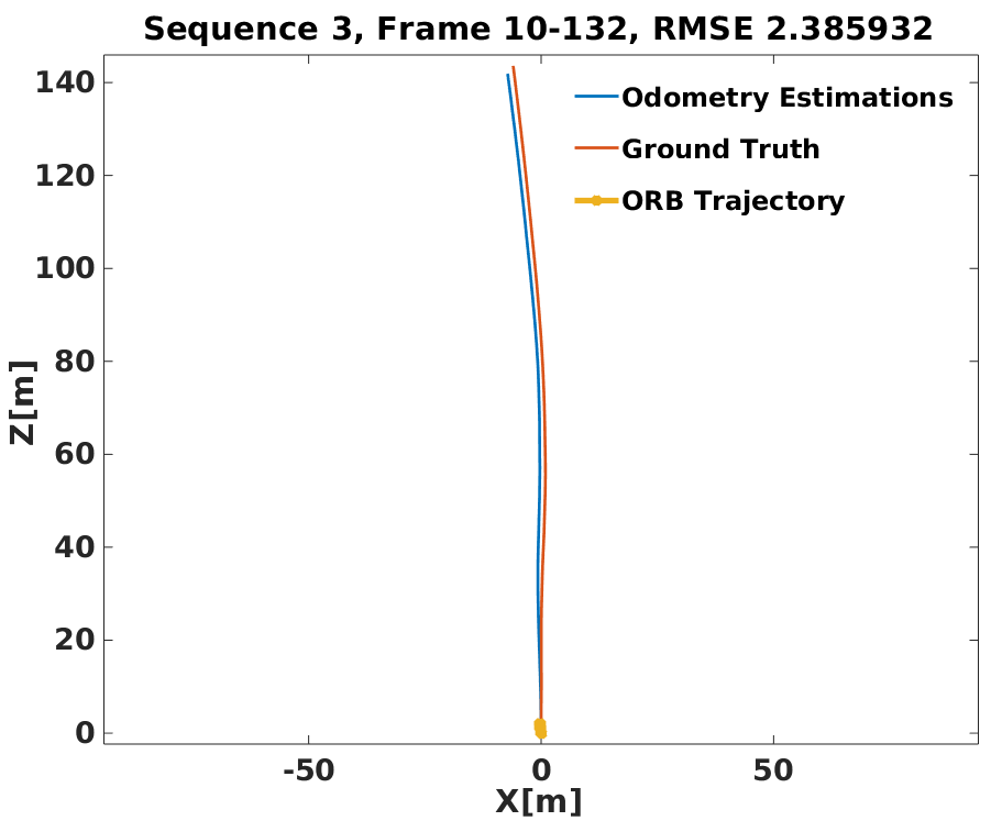
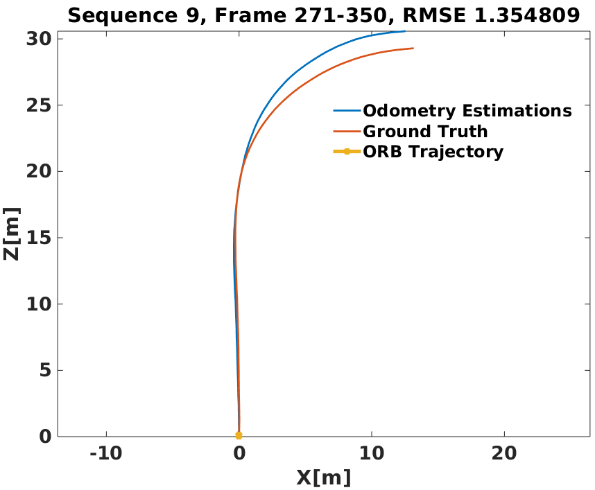
For accurate visual odometry, we exploit distinguishable static ORB[2, 26] features on the road plane from entities like curbs, lane markers and any irregularities on the road to obtain quality point correspondences. While the approach is dependent on factors like reasonable visibility, we obtain robust performance over a diverse range of sequences many of which are over a 100 frames long. Fig. 7 illustrates how our method achieves a fairly accurate scaling of odometry to provide an initialization that competes well with the corresponding ground truth.
VI-B3 Pose-Graph Optimization
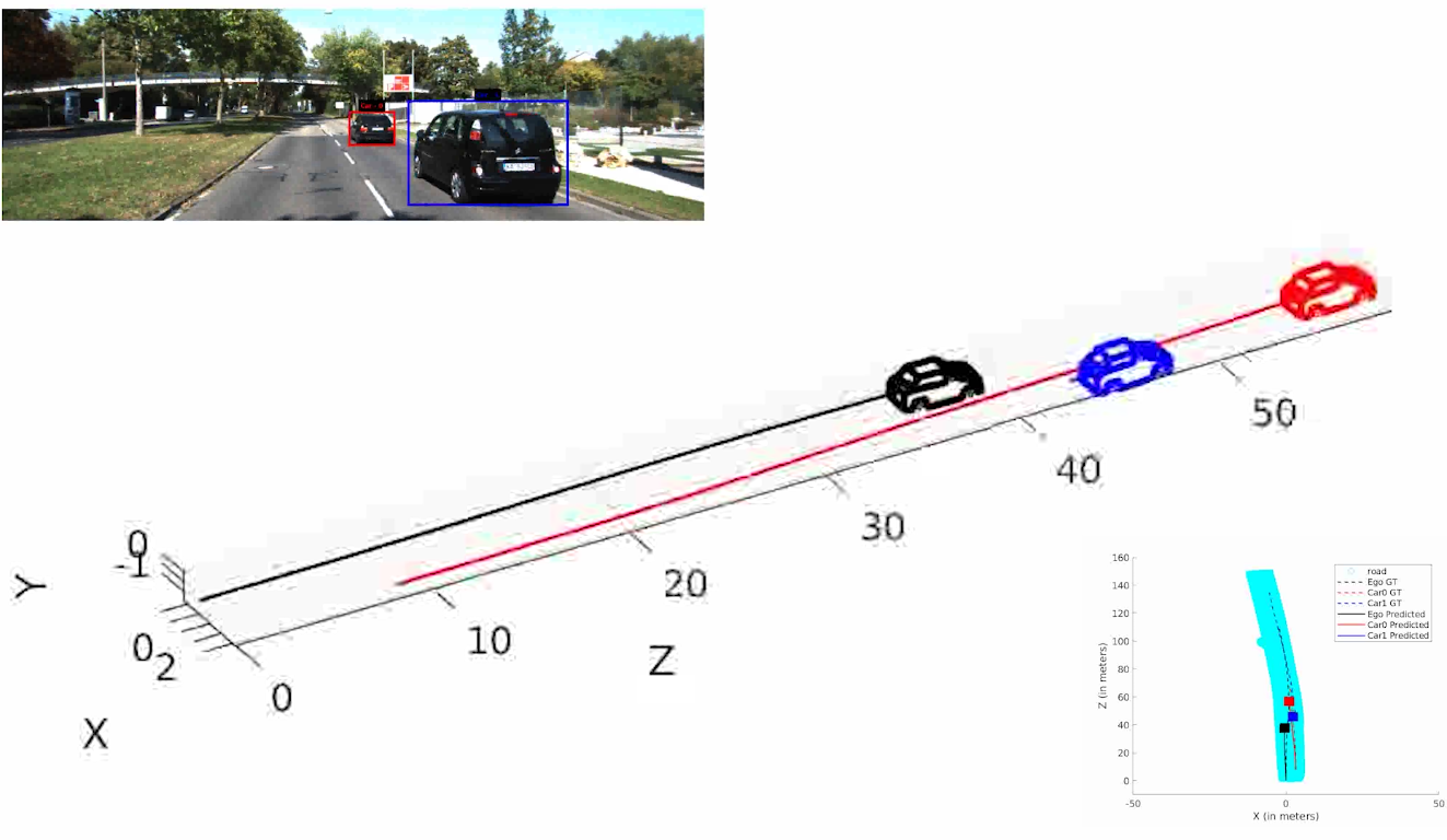
We resolve for each cyclic-loop created by the ego-camera and each vehicle (cf. Eqn. 14) in the scene in our optimization formulation. The optimization problem runs for a maximum of 100 iterations. Our optimization formulation performs consistently well on a wide range of sequences irrespective of the sequence length, number of objects in the scene and varying object instance lengths. A unique pose-graph structure for all vehicles including ego-motion at each time instance ensures effective error re-distribution across all trajectories based on efficient confidence parameterization (cf. Eqn. 15). Fig. 5 illustrates ego-motion as well as the motion of various vehicles over many sequences from the KITTI Tracking dataset[1].
VI-C Quantitative Results
VI-C1 Odometry Estimations
As an attempt to improve odometry estimations, we place a threshold T on the depth from camera upto which we consider point correspondences. This has been set based on our observation that the accuracy of the 3D depth to the point correspondences lowers with depth from the camera. Table I summarizes our experiments with various threshold values before we finalize our threshold at T = 12 metres.
Seq no. Seq length Threshold (metres) Average ATE
Absolute Translation Error (Root Mean Square) in Global Frame (metres) Seq No. 3 4 18 Avg Error Car ID Ego-car Ego-car Ego-car Frame length Namdev et al.[12] Ours
Absolute Translation Error (ATE) (Root Mean Square) in Global Frame (metres) Seq number 3 4 18 Avg Error Car ID Ego-car Ego-car Ego-car Frame length Initialization Only C-C and C-V edges Only C-C and V-V edges Only C-V and V-V edges With C-C, C-V and V-V edges Percentage Errors
While T = 12 meters delivers best results for most sequences mentioned in Table I, we see that T = 15 metres performs better for sequences 6 and 9, both of which involve the ego-vehicle taking a sharp turn at an intersection. This is because we rely on ground plane features including and largely contributed to by the lane markers on the road plane. Given that the segment of road plane in the scene at an intersection is devoid of any road/lane markers, we do not get enough feature correspondences from closer segments of the road. Meanwhile, increasing the threshold enables us to pick up points from the road plane continuing beyond the intersection which contains better scope for quality feature correspondences in the form of lane markers. Consequently, a relatively larger threshold performs better.
VI-C2 Pose-Graph Optimization
Our pose-graph formulation consists of three categories of edges namely camera-camera(C-C) edges, camera-vehicle(C-V) edges and Vehicle-Vehicle(V-V) edges. Each of these sets of edges are accompanied by a unique confidence parameter . To understand the contribution category of edges to our pose-graph optimization, we analyse the results on removing these constraints. Table III summarizes our observations. It can be noted that few vehicles in sequence 3 and the ego-vehicle in sequence 4 perform better when C-C constraints are relaxed. This is because, the optimizer generally utilizes reliable edges in each loop of the pose-graph to improve the relatively less reliable edges, provided their information matrices are scaled appropriately. Given that the C-C edges are less reliable in these sequences, relaxing its constraints enables other edges to improve upon the overall error. A similar explanation can be given for the errors for ego-motion in sequence 18. Since C-C edges of the ego-motion in sequence 18 are more accurate than the corresponding C-V edges of other vehicles, we obtain a better result for the same when the C-V edge constraint is relaxed. Both C-C and V-V edges are generated using the odometry estimations and are influenced by its accuracy too.
VI-D Summary of Results
While Fig. 5 illustrates how our trajectories perform with respect to the ground truth, Table III reaffirms how our pose-graph formulation successfully redistributes errors about constraints with high confidence parameters. Table II reports our pipeline’s performance with respect to Namdev et al.[12]. Tables III and II vindicate the efficacy of the proposed pipeline as the absolute translation error(ATE) are typically around 3m for sequences more than 100m in length. The last row of Table III denotes the percentage error, which is significantly low for fairly long sequences at an average of 3.11%, considering that the original problem is intractable and hard to solve.
VII Conclusion
Monocular Multi-body SLAM is ill-posed as it is impossible to triangulate a moving vehicle from a moving monocular camera. This observability problem manifests in the form of relative scale when posed into the Multibody framework. With the arrival of single view reconstruction methods based on Deep Learning, some of these difficulties are alleviated, but one is still entailed to represent the camera motion and the vehicles in the same scale. This paper solves for this scale by making use of the ground plane features thereby initializing the ego vehicle and other dynamic participants with respect to a unified frame in metric scale. Further, a pose graph optimization over vehicle poses between successive frames mediated by the camera motion formalizes the Multibody SLAM framework.
We showcase trajectories of dynamic participants and the ego vehicle over sequences of more than a hundred frames in length with high fidelity ATE (Absolute Translation Error). To the best of our knowledge, this is the first such method to represent vehicle trajectories in the global frame over long sequences. The pipeline is able to accurately map trajectories of dynamic participants far away from the ego camera and its scalability to map multi-vehicle trajectories is another salient aspect of this work.
References
- [1] A. Geiger, P. Lenz, C. Stiller, and R. Urtasun, “Vision meets robotics: The kitti dataset,” IJRR, 2013.
- [2] M. J. M. M. Mur-Artal, Raúl and J. D. Tardós, “ORB-SLAM: a versatile and accurate monocular SLAM system,” IEEE Transactions on Robotics, 2015.
- [3] J. Engel, T. Schöps, and D. Cremers, “LSD-SLAM: Large-scale direct monocular SLAM,” in ECCV, 2014.
- [4] C. Forster, Z. Zhang, M. Gassner, M. Werlberger, and D. Scaramuzza, “Svo: Semidirect visual odometry for monocular and multicamera systems,” IEEE Transactions on Robotics, 2017.
- [5] K. Ozden, Kemal E anld Schindler and L. Van Gool, “Multibody structure-from-motion in practice,” PAMI, 2010.
- [6] A. J. Davison, I. D. Reid, N. Molton, and O. Stasse, “Monoslam: Real-time single camera slam,” IEEE Transactions on Pattern Analysis and Machine Intelligence, 2007.
- [7] A. Kundu, K. M. Krishna, and C. Jawahar, “Realtime multibody visual slam with a smoothly moving monocular camera,” in ICCV, 2011.
- [8] K. E. Ozden, K. Cornelis, L. V. Eycken, and L. V. Gool", “Reconstructing 3d trajectories of independently moving objects using generic constraints,” CVIU, 2004.
- [9] R. Vidal, Y. Ma, S. Soatto, and S. Sastry, “Two-view multibody structure from motion,” IJCV, 2006.
- [10] K. Schindler and D. Suter, “Two-view multibody structure-and-motion with outliers through model selection,” PAMI, 2006.
- [11] S. R. Rao, A. Y. Yang, S. S. Sastry, and Y. Ma, “Robust algebraic segmentation of mixed rigid-body and planar motions from two views,” IJCV, 2010.
- [12] R. Namdev, K. M. Krishna, and C. V. Jawahar, “Multibody vslam with relative scale solution for curvilinear motion reconstruction,” in ICRA, 2013.
- [13] J. Costeira and T. Kanade, “A multi-body factorization method for motion analysis,” in ICCV, 1995.
- [14] A. W. Fitzgibbon and A. Zisserman, “Multibody structure and motion: 3-d reconstruction of independently moving objects,” in ECCV, 2000.
- [15] M. Han and T. Kanade, “Multiple motion scene reconstruction from uncalibrated views,” in ICCV, 2001.
- [16] M. Machline, L. Zelnik-Manor, and M. Irani, “Multi-body segmentation: Revisiting motion consistency,” in ECCV Workshop on Vision and Modeling of Dynamic Scenes, 2002.
- [17] S. Avidan and A. Shashua, “Trajectory triangulation: 3d reconstruction of moving points from a monocular image sequence,” PAMI, 2000.
- [18] R. Ranftl, V. Vineet, Q. Chen, and V. Koltun, “Dense monocular depth estimation in complex dynamic scenes,” in CVPR, 2016.
- [19] S. Yang and S. Scherer, “Cubeslam: Monocular 3-d object slam,” IEEE Transactions on Robotics, 2019.
- [20] S. Rota Bulò, L. Porzi, and P. Kontschieder, “In-place activated batchnorm for memory-optimized training of dnns,” in CVPR, 2018.
- [21] K. He, G. Gkioxari, P. Dollár, and R. Girshick, “Mask r-cnn,” in ICCV, 2017.
- [22] R. Girshick, “Fast r-cnn,” in ICCV, 2015.
- [23] S. Ren, K. He, R. Girshick, and J. Sun, “Faster r-cnn: Towards real-time object detection with region proposal networks,” in Advances in neural information processing systems, 2015.
- [24] N. D. Reddy, I. Abbasnejad, S. Reddy, A. K. Mondal, and V. Devalla, “Incremental real-time multibody vslam with trajectory optimization using stereo camera,” in IROS, 2016.
- [25] P. Li, T. Qin, et al., “Stereo vision-based semantic 3d object and ego-motion tracking for autonomous driving,” in ECCV, 2018.
- [26] R. Mur-Artal and J. D. Tardós, “Orb-slam2: An open-source slam system for monocular, stereo, and rgb-d cameras,” IEEE Transactions on Robotics, 2017.
- [27] J. Redmon and A. Farhadi, “Yolo9000: Better, faster, stronger,” in CVPR, 2017.
- [28] S. Song and M. Chandraker, “Joint sfm and detection cues for monocular 3d localization in road scenes,” in CVPR, 2015.
- [29] J. K. Murthy, S. Sharma, and K. M. Krishna, “Shape priors for real-time monocular object localization in dynamic environments,” in IROS, 2017.
- [30] J. K. Murthy, G. S. Krishna, F. Chhaya, and K. M. Krishna, “Reconstructing vehicles from a single image: Shape priors for road scene understanding,” in ICRA, 2017.
- [31] J. A. Ansari, S. Sharma, A. Majumdar, J. K. Murthy, and K. M. Krishna, “The earth ain’t flat: Monocular reconstruction of vehicles on steep and graded roads from a moving camera,” in IROS, 2018.
- [32] A. Newell, K. Yang, and J. Deng, “Stacked hourglass networks for human pose estimation,” in ECCV, 2016.
- [33] G. Grisetti, R. Kümmerle, H. Strasdat, and K. Konolige, “g2o: a general framework for (hyper) graph optimization,” in ICRA, 2011.