This paper was converted on www.awesomepapers.org from LaTeX by an anonymous user.
Want to know more? Visit the Converter page.

Multi-Objective Complementary Control

Jiapeng Xu, Xiang Chen, Ying Tan, and Kemin Zhou Jiapeng Xu and Xiang Chen are with the Department of Electrical and Computer Engineering, University of Windsor, 401 Sunset Avenue, Windsor, ON N9B 3P4, Canada (e-mails: imxjp@sina.com; xchen@uwindsor.ca).Ying Tan is with the Department of Mechanical Engineering, The University of Melbourne, Melbourne, VIC 3010, Australia (e-mail: yingt@unimelb.edu.au).Kemin Zhou is with the Center for Advanced Control and Smart Operations, Nanjing University, Suzhou, Jiangsu 215163, China (e-mail: kmzhou@nju.edu.cn).
Abstract

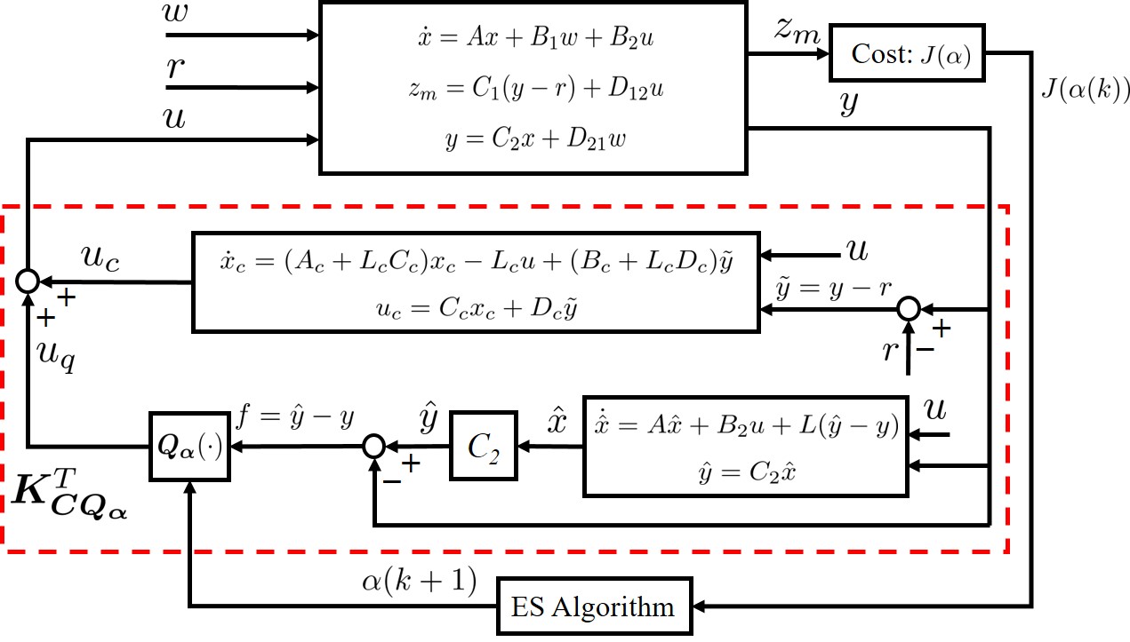
This paper proposes a novel multi-objective control framework for linear time-invariant systems in which performance and robustness can be achieved in a complementary way instead of a trade-off. In particular, a state-space solution is first established for a new stabilizing control structure consisting of two independently designed controllers coordinated with a Youla-type operator 𝑸{\bm{Q}}. It is then shown by performance analysis that these two independently designed controllers operate in a naturally complementary way for a tracking control system, due to the coordination function of 𝑸{\bm{Q}} driven by the residual signal of a Luenberger observer. Moreover, it is pointed out that 𝑸{\bm{Q}} could be further optimized with an additional gain factor to achieve improved performance, through a data-driven methodology for a measured cost function.

Index Terms:
Multi-objective control, complementary control, Youla-Kučera parameterization, robustness

I Introduction

There are usually multiple objectives or specifications required to be achieved by various control systems in practice [1, 2, 3, 4, 5, 6, 7, 8, 9], such as optimality of tracking performance, robustness to some unknown/uncertain disturbances or parameter variations, passivity, etc. Various formulated multi-objective (MO) control problems have received considerable attention in the control community, for example, the MO 2/\mathcal{H}_{2}/\mathcal{H}_{\infty} control [10, 11, 12, 13, 14, 15, 4], where optimization of performance in the 2\mathcal{H}_{2} norm and robustness in the \mathcal{H}_{\infty} norm are considered simultaneously and are heavily studied in 1990’s. Other kinds of MO optimal control problems have also been extensively explored, for example, in [1, 3, 15, 7, 6], where the concept of Pareto optimality is used with respect to multiple optimization criteria.

It can be observed that the common feature of these traditional MO control problems is the fact that a single-controller structure is applied which poses challenges for the design methodologies, especially, when the involved objectives are inherently conflicting. A typical example is the well-known conflicting pair of robustness and optimal performance in a traditional robust control design. When conflicting objectives could not be achieved at their best by the single controller, the trade-off is normally the only choice, which results in a compromised single controller, as can be seen in many mixed 2/\mathcal{H}_{2}/\mathcal{H}_{\infty} control results [10, 11, 12, 14, 15, 4]. There are some research reported for controller designs in the two-degree-of-freedom (2DoF) form [16, 17, 18]. The reference [16] is concerned with 2DoF optimal design for a quadratic cost. In particular, the class of all stabilizing 2DoF controllers which give finite cost is characterized. In [17], the class of all stabilizing 2DoF controllers which achieve a specified closed-loop transfer matrix is characterized in terms of a free stable parameter. Inspired by the generalized internal model control (GIMC) developed in [19], a bi-objective high-performance control design for antenna servo systems is studied in [18]. Performance limitation problems are also studied for 2DoF controllers in [20, 21], with tracking and/or regulation as a sole objective. However, there is, essentially, a lack of a fundamental and general framework that can assemble two controllers together in a complementary way for MO control design purposes. That said, it is desired to develop a new framework for MO control problems that can overcome the curse of trade-offs and achieve non-compromised MO performances, which is the main goal of this paper.

This work is closely related to the GIMC structure [19], a multi-block implementation of the famous Youla-Kučera parameterization of all stabilizing 1DoF and 2DoF controllers [22]. In this implementation, the Youla-type parameter 𝑸(s)\bm{Q}(s) becomes an explicit design factor driven by the residual signal, instead of functioning as an optional parameter to deliver a specific stabilizing controller. Although this GIMC structure provides hope for the desired two-controller complementary structure to address MO control problems, no further details are given for the systematic design of 𝑸(s)\bm{Q}(s) in [19]. Motivated by the GIMC, in this paper a new two-controller design framework called ‘Multi-Objective Complementary Control’ (MOCC) is proposed and explored in detail with rigorous performance analysis, aiming to achieve MO performances while alleviating trade-offs. In particular, state-space formulas are provided for the MOCC framework. A tracking control setting is utilized as a platform to demonstrate the said advantages of MOCC, that is, overcoming the trade-off in the conventional MO control to achieve nominal tracking performance and robustness in a complementary way. Furthermore, a data-driven optimization approach is also sketched for the design of Youla-type operator 𝑸\bm{Q} to turn a robust controller into an optimal one, when performing the tracking task repetitively over a finite time interval in the presence of an unknown but repetition-invariant disturbance.

This paper is organized as follows: in Section II, the motivation of this paper is explained in detail using a tracking control case as well as some preliminaries of GIMC and Youla-Kučera parameterization; Section III presents a new two-controller structure which enables the MOCC design in the later section; in Section IV, a tracking control problem is addressed in the new framework with a rigorous performance analysis, illustrating the design features and the advantages of MOCC; the data-driven performance optimization is sketched in Section V; simulation results can be found in Section VI and conclusions in Section VII.

Notations: Throughout this paper, the symbol of transfer matrices or systems will be in bold to distinguish them from constant matrices. A system and its transfer function are denoted by the same symbol and whenever convenient, the dependence on the frequency variable ss or jωj\omega for a transfer function may be omitted. The set n\mathbb{R}^{n} consists of all nn-dimensional real vectors. The unsubscripted norm \|\cdot\| denotes the standard Euclidean norm on vectors. For a matrix or vector XX, XX^{\prime} denotes its transpose. For a rational transfer matrix 𝑻(s)\bm{T}(s), 𝑻\bm{T}^{*} denotes 𝑻(s)\bm{T}^{\prime}(-s) or complex conjugation of 𝑻(jω)\bm{T}(j\omega). \mathcal{RL}_{\infty} (\mathcal{RH}_{\infty}) denotes the space of all rational (and stable) functions with the norm 𝑻(s)=supωσ¯{𝑻(jω)}\displaystyle{\|\bm{T}(s)\|_{\infty}=\sup_{\omega}\bar{\sigma}\{\bm{T}(j\omega)\}} for any 𝑻(s)()\bm{T}(s)\in\mathcal{RL}_{\infty}(\mathcal{RH}_{\infty}), where σ¯{}\bar{\sigma}\{\cdot\} represents the largest singular value. A rational proper transfer matrix in terms of state-space data is simply denoted by [ABCD]:=C(sIA)1B+D\left[\begin{array}[]{c|c}A&B\\ \hline\cr C&D\end{array}\right]:=C(sI-A)^{-1}B+D.

II Motivation

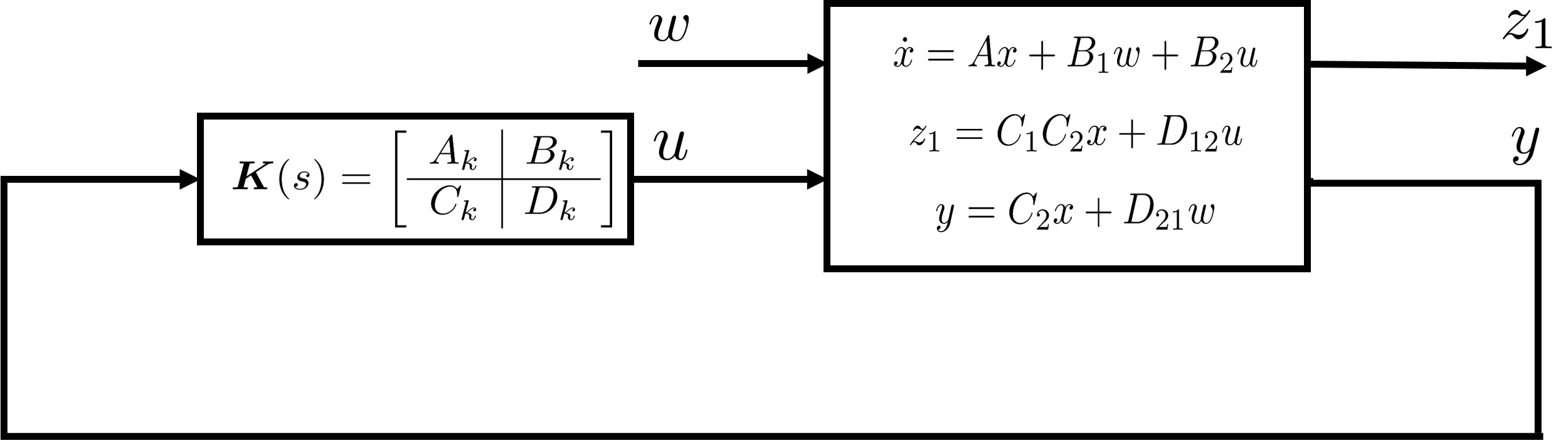
Transfer functions shall be utilized to motivate our idea, though this paper mainly works on state space. Consider a tracking control system shown in Fig. 1. Let 𝑮(s)=𝑴~1(s)𝑵~(s)\bm{G}(s)=\bm{\tilde{M}}^{-1}(s)\bm{\tilde{N}}(s) be a linear time-invariant (LTI) plant with a left coprime factorization 𝑴~(s)\bm{\tilde{M}}(s)\in{\cal RH}_{\infty} and 𝑵~(s)\bm{\tilde{N}}(s)\in{\cal RH}_{\infty}, 𝑪(s)=𝑽~1(s)𝑼~(s)\bm{C}(s)=\bm{\tilde{V}}^{-1}(s)\bm{\tilde{U}}(s) be a stabilizing controller with a left coprime factorization 𝑽~(s)\bm{\tilde{V}}(s)\in{\cal RH}_{\infty} and 𝑼~(s)\bm{\tilde{U}}(s)\in{\cal RH}_{\infty}, 𝒓(s)\bm{r}(s) be a reference signal to be tracked, and 𝒘(s)\bm{w}(s) be an uncertain or unknown disturbance signal. It is well-known that all stabilizing controllers can be characterized in the format of Youla-Kučera parameterization

𝑲=(𝑽~𝑸𝑵~)1(𝑼~+𝑸𝑴~)\displaystyle\bm{K}=(\bm{\tilde{V}}-\bm{Q}\bm{\tilde{N}})^{-1}(\bm{\tilde{U}}+\bm{Q}\bm{\tilde{M}})

for the same plant 𝑮(s)\bm{G}(s), with 𝑸(s)\bm{Q}(s)\in{\cal RH}_{\infty} and det(𝑽~()𝑸()𝑵~())0{\rm det}(\bm{\tilde{V}}(\infty)-\bm{Q}(\infty)\bm{\tilde{N}}(\infty))\neq 0 [19], [22, Chapter 5], [23]. The tracking error 𝒆(s)=𝒓(s)𝒚(s)\bm{e}(s)=\bm{r}(s)-\bm{y}(s) with either 𝑪(s)\bm{C}(s) or 𝑲(s)\bm{K}(s) is given by

𝒆\displaystyle\bm{e} =(I+𝑮𝑪)1𝒓(I+𝑮𝑪)1𝑮𝒘,\displaystyle=(I+\bm{G}\bm{C})^{-1}\bm{r}-(I+\bm{G}\bm{C})^{-1}\bm{G}\bm{w},
or𝒆\displaystyle\text{or}\;\bm{e} =(I+𝑮𝑲)1𝒓(I+𝑮𝑲)1𝑮𝒘.\displaystyle=(I+\bm{G}\bm{K})^{-1}\bm{r}-(I+\bm{G}\bm{K})^{-1}\bm{G}\bm{w}.

It can be seen that the single controller 𝑪(s)\bm{C}(s) (or 𝑲(s)\bm{K}(s)) has to be designed to deal with both the tracking performance for the reference signal 𝒓(s)\bm{r}(s) and the robustness against the disturbance 𝒘(s)\bm{w}(s) simultaneously. In practice, trade-off usually should be carried out to compromise the design difficulty of the single 𝑪(s)\bm{C}(s) (or 𝑲(s)\bm{K}(s)) between the tracking performance and the disturbance attenuation. On the other hand, considering the challenge posed for the selection of 𝑸(s)\bm{Q}(s) under a given performance expectation of 𝑲(s)\bm{K}(s), one can conclude that finding a 𝑲(s)\bm{K}(s) is not necessarily easier than designing 𝑪(s)\bm{C}(s) when both performance and robustness need to be addressed.

Refer to caption
Figure 1: Tracking control system.

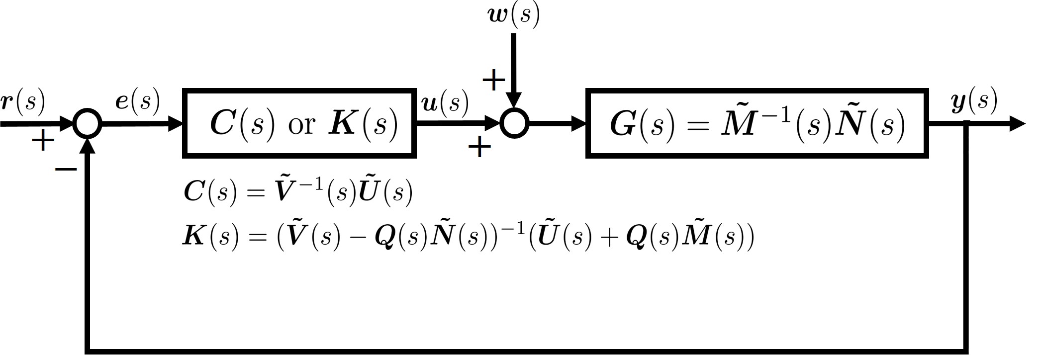
An interesting controller architecture called GIMC was proposed in [19] which provides a promising approach to overcome the trade-off in the traditional design. The GIMC is shown in Fig. 2, featuring the parameter 𝑸(s)\bm{Q}(s)\in{\cal RH}_{\infty} as a separate design factor in the structure, instead of being buried in 𝑲(s)\bm{K}(s). By direct algebra, the tracking error 𝒆(s)\bm{e}(s) in Fig. 2 can be derived as

𝒆=\displaystyle\bm{e}= (I+𝑮𝑪)1𝒓(I+𝑮𝑪)1𝑮(I𝑽~1𝑸𝑵~)𝒘.\displaystyle(I+\bm{G}\bm{C})^{-1}\bm{r}-(I+\bm{G}\bm{C})^{-1}\bm{G}(I-\bm{\tilde{V}}^{-1}\bm{Q}\bm{\tilde{N}})\bm{w}.

It is clear from the above expression that different from the control structure in Fig. 1, there are potentially two separate design degrees of freedom for tracking control in GIMC: 𝑪(s)\bm{C}(s) for tracking performance and 𝑸(s)\bm{Q}(s) for disturbance attenuation. In addition, if there is no uncertainty, i.e., 𝒘=0\bm{w}=0, then 𝒆=(I+𝑮𝑪)1𝒓\bm{e}=(I+\bm{G}\bm{C})^{-1}\bm{r} and thus the nominal tracking error signal is recovered. These attractive features motivate us to revisit MO control problems through the design of 𝑪(s)\bm{C}(s) and 𝑸(s)\bm{Q}(s), instead of the traditional design of a single controller 𝑪(s)\bm{C}(s) or 𝑲(s)\bm{K}(s). Noting that, for a given 𝑪(s)\bm{C}(s), if 𝑸(s)\bm{Q}(s) can be determined then 𝑲(s)\bm{K}(s) is derived and vice verse. Hence, design of 𝑪(s)\bm{C}(s) and 𝑸(s)\bm{Q}(s) can be reduced to the design of 𝑪(s)\bm{C}(s) and 𝑲(s)\bm{K}(s) even if 𝑲(s)\bm{K}(s) is not explicitly seen in Fig 2. It is noted that how to coordinate 𝑪(s)\bm{C}(s) and 𝑲(s)\bm{K}(s) using 𝑸(s)\bm{Q}(s) such that specified performances are achieved and rigorous performance analysis for GIMC have not systematically and profoundly been investigated so far. In [24], a solution to 𝑸(s)\bm{Q}(s) is derived in state space for a robust LQG control problem through the \mathcal{H}_{\infty} design with a modified control structure from GIMC, although it is still not clear how to systematically use 𝑸(s)\bm{Q}(s) to coordinate 𝑪(s)\bm{C}(s) and 𝑲(s)\bm{K}(s) in the Youla-Kučera parameterization.

Refer to caption
Figure 2: Generalized internal model control (GIMC) structure.

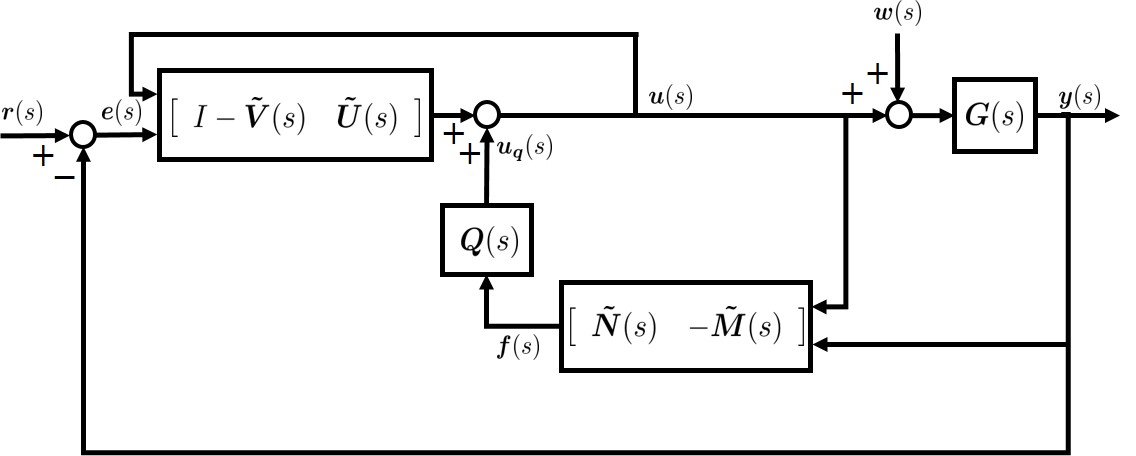
In the following sections of this paper, a two-controller structure 𝑲𝑪𝑸\bm{K_{CQ}} is proposed in state space, motivated from the analysis above. In particular, how 𝑸\bm{Q} can be constructed from two independently designed controllers 𝑪\bm{C} and 𝑲\bm{K} to coordinate 𝑪\bm{C} and 𝑲\bm{K} is explored systematically. To showcase the superior performance of this new control design framework, a tracking control problem is presented to demonstrate how 𝑪\bm{C} and 𝑲\bm{K} can be coordinated through 𝑸\bm{Q} to address MO tracking performance and robustness in a complementary way, together with a rigorous performance analysis.

Remark 1

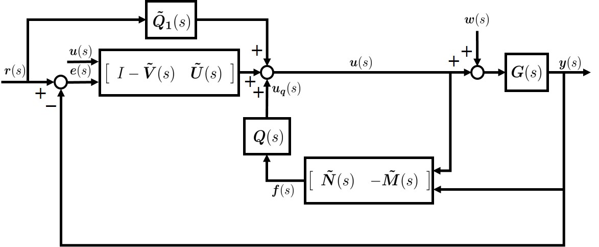
Note that the GIMC structure in Fig. 2 can be extended to an equivalent 2DoF controller structure with an additional feed-forward parameter 𝐐~𝟏(s)\bm{\tilde{Q}_{1}}(s)\in\mathcal{RH_{\infty}}, shown in Fig 3. Indeed, the controller in Fig. 3 can be deemed as 𝐮=𝐊𝟏𝐫𝐊𝟐𝐲\bm{u}=\bm{K_{1}r}-\bm{K_{2}y} with

[𝑲𝟏𝑲𝟐]=(𝑽~𝑸𝑵~)1[𝑼~+𝑸~𝟏(𝑼~+𝑸𝑴~)],\displaystyle\left[\begin{array}[]{cc}\bm{K_{1}}&\bm{K_{2}}\end{array}\right]=(\bm{\tilde{V}}-\bm{Q}\bm{\tilde{N}})^{-1}\left[\begin{array}[]{cc}\bm{\tilde{U}}+\bm{\tilde{Q}_{1}}&(\bm{\tilde{U}}+\bm{Q}\bm{\tilde{M}})\end{array}\right],

which in fact parameterizes all stabilizing 2DoF controllers in terms of free parameters 𝐐~𝟏(s)\bm{\tilde{Q}_{1}}(s)\in\mathcal{RH_{\infty}} and 𝐐(s)\bm{Q}(s)\in\mathcal{RH_{\infty}} [22, Theorem 5.6.3]. In this case, the controller 𝐂(s)\bm{C}(s) can be obtained as 𝐕~1[𝐔~+𝐐~𝟏𝐔~]\bm{\tilde{V}}^{-1}\left[\begin{array}[]{cc}\bm{\tilde{U}}+\bm{\tilde{Q}_{1}}&\bm{\tilde{U}}\end{array}\right]. Since 𝐐~𝟏(s)\bm{\tilde{Q}_{1}}(s)\in\mathcal{RH_{\infty}} occurs in the feed-forward channel, without loss of generality, the GIMC in Fig. 2 is adopted as the beginning structure in this paper. \Box

Refer to caption
Figure 3: A GIMC implementation of 2DOF controller.

III Two-Controller Structure

This section presents a new stabilizing control structure motivated by GIMC. Consider the following finite-dimensional linear time-invariant (FDLTI) system

𝑮:{x˙=Ax+B2uy=C2x,\displaystyle\bm{G}:\left\{\mspace{-6.0mu}\begin{array}[]{l}\dot{x}=Ax+B_{2}u\\ y=C_{2}x,\end{array}\right. (3)

where xnx\in\mathbb{R}^{n}, um2u\in\mathbb{R}^{m_{2}} and yp2y\in\mathbb{R}^{p_{2}} are the state, control input, and sensor output, respectively. All matrices are real constant and have compatible dimensions. The following assumption is required throughout the remainder of this paper.

Assumption 1

(A,B2)(A,B_{2}) is stabilizable and (C2,A)(C_{2},A) is detectable.

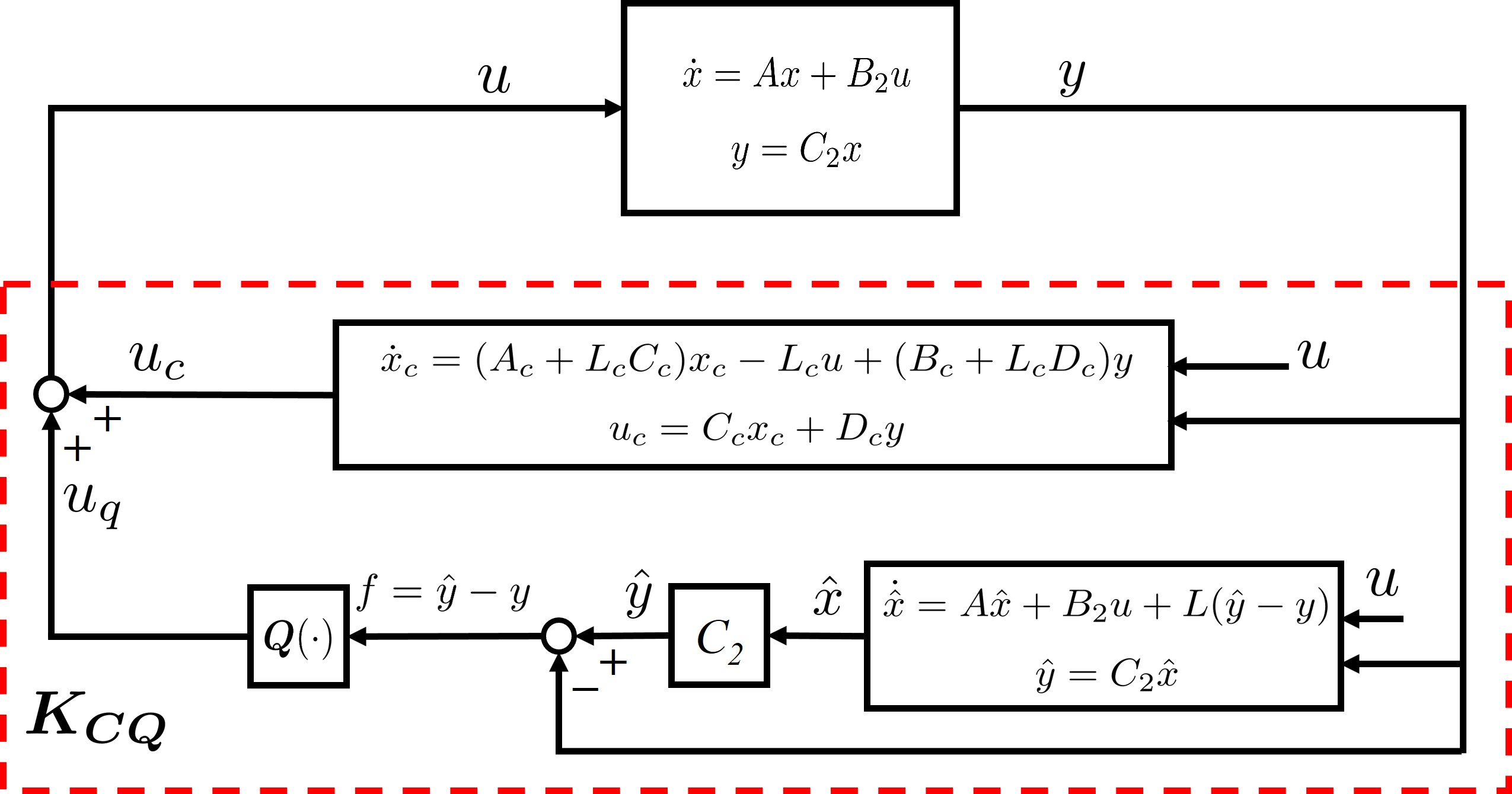
A full-order Luenberger observer for system (3) can be given by

x^˙\displaystyle\dot{\hat{x}} =Ax^+B2u+Lf,\displaystyle=A\hat{x}+B_{2}u+Lf, (4)

where f=C2x^yf=C_{2}\hat{x}-y is the residual signal and LL is any matrix such that A+LC2A+LC_{2} is stable. Note that the Luenberger observer (4) is very related to the GIMC structure in Fig. 2. Specifically, by letting 𝑮(s):=[AB2C20]\bm{G}(s):=\left[\begin{array}[]{c|c}A&B_{2}\\ \hline\cr C_{2}&0\end{array}\right] in the GIMC structure, a state-space realization of 𝑴~(s)\bm{\tilde{M}}(s) and 𝑵~(s)\bm{\tilde{N}}(s) can be obtained as

[𝑵~(s)𝑴~(s)]=[A+LC2B2LC20I],\displaystyle\left[\begin{array}[]{cc}\bm{\tilde{N}}(s)&\bm{\tilde{M}}(s)\end{array}\right]=\left[\begin{array}[]{c|cc}A+LC_{2}&B_{2}&L\\ \hline\cr C_{2}&0&I\end{array}\right],

and it is not difficult to observe that 𝒇(s)=𝑵~(s)𝒖(s)𝑴~(s)𝒚(s)\bm{f}(s)=\bm{\tilde{N}}(s)\bm{u}(s)-\bm{\tilde{M}}(s)\bm{y}(s) is the residual signal generated by the Luenberger observer (4).

For the system 𝑮\bm{G} in (3), consider a dynamic output-feedback stabilizing controller 𝑪\bm{C}:

𝑪:{x˙c=Acxc+Bcyuc=Ccxc+Dcy.\displaystyle{\bm{C}}:\left\{\mspace{-6.0mu}\begin{array}[]{l}\dot{x}_{c}=A_{c}x_{c}+B_{c}y\\ u_{c}=C_{c}x_{c}+D_{c}y.\end{array}\right. (7)

Clearly, (Ac,Bc,Cc)(A_{c},B_{c},C_{c}) is stabilizable and detectable, since 𝑪\bm{C} stabilizes 𝑮\bm{G} if and only if 𝑮\bm{G} stabilizes 𝑪\bm{C} [22, Section 5.1]. Then there exists a matrix LcL_{c}, such that Ac+LcCcA_{c}+L_{c}C_{c} is stable. Motivated from the GIMC structure in Fig. 2, we present the following composite controller 𝑲𝑪𝑸\bm{K_{CQ}}:

𝑲𝑪𝑸:{x˙c=(Ac+LcCc)xcLcu+(Bc+LcDc)yuc=Ccxc+Dcyx^˙=Ax^+B2u+Lfuq=𝑸(f)u=uc+uq\displaystyle\bm{K_{CQ}}:\left\{\mspace{-6.0mu}\begin{array}[]{l}\dot{x}_{c}=(A_{c}+L_{c}C_{c})x_{c}-L_{c}u+(B_{c}+L_{c}D_{c})y\\ u_{c}=C_{c}x_{c}+D_{c}y\\ \dot{\hat{x}}=A\hat{x}+B_{2}u+Lf\\ u_{q}={\bm{Q}}(f)\\ u=u_{c}+u_{q}\end{array}\right. (13)

based on the observer (4) and the controller 𝑪{\bm{C}} in (7), where 𝑸(){\bm{Q}}(\cdot) is a stable dynamic operator driven by the residual signal ff to be designed in the following form:

𝑸:{x˙q=Aqxq+Bqfuq=Cqxq+Dqf\displaystyle{\bm{Q}}:\left\{\mspace{-6.0mu}\begin{array}[]{l}\dot{x}_{q}=A_{q}x_{q}+B_{q}f\\ u_{q}=C_{q}x_{q}+D_{q}f\end{array}\right. (16)

with AqA_{q} stable.

The significant feature of the composite controller 𝑲𝑪𝑸\bm{K_{CQ}} is that if the output signal uqu_{q} of 𝑸{\bm{Q}} is zero, then u=ucu=u_{c} and 𝑲𝑪𝑸\bm{K_{CQ}} is the same as the controller 𝑪\bm{C} in (7). On the other hand, if uq0u_{q}\neq 0, then the composite controller 𝑲𝑪𝑸\bm{K_{CQ}} behaves like a different one. Therefore, 𝑲𝑪𝑸\bm{K_{CQ}} can be viewed as a two-controller structure to stabilize the system 𝑮\bm{G} in (3), as shown in Fig. 4.

Refer to caption
Figure 4: Two-controller structure.

Now consider another dynamic output-feedback stabilizing controller 𝑲{\bm{K}} designed in the following form:

𝑲:{x˙k=Akxk+Bkyuk=Ckxk+Dky.\displaystyle{\bm{K}}:\left\{\mspace{-6.0mu}\begin{array}[]{l}\dot{x}_{k}=A_{k}x_{k}+B_{k}y\\ u_{k}=C_{k}x_{k}+D_{k}y.\end{array}\right. (19)

Then we give the solution of 𝑸\bm{Q} in state space such that 𝑲𝑪𝑸=𝑲\bm{K_{CQ}}=\bm{K} when uq0u_{q}\neq 0, which is presented in the following proposition.

Proposition 1

Given two arbitrarily designed stabilizing controllers 𝐂\bm{C} in (7) and 𝐊\bm{K} in (19) and letting LL and LcL_{c} be any matrices such that both A+LC2A+LC_{2} and Ac+LcCcA_{c}+L_{c}C_{c} are stable, then a stable 𝐐{\bm{Q}} in (16) can be realized with

Aq\displaystyle A_{q} =[Ac+LcCc(Bc+LcDq)C2LcCk0A+B2DkC2B2Ck0BkC2Ak],\displaystyle=\left[\begin{array}[]{ccc}A_{c}+L_{c}C_{c}&(B_{c}+L_{c}D_{q})C_{2}&-L_{c}C_{k}\\ 0&A+B_{2}D_{k}C_{2}&B_{2}C_{k}\\ 0&B_{k}C_{2}&A_{k}\end{array}\right], (23)
Bq\displaystyle B_{q} =[BcLcDqLB2DkBk],\displaystyle=\left[\begin{array}[]{ccc}-B_{c}-L_{c}D_{q}\\ L-B_{2}D_{k}\\ -B_{k}\end{array}\right], (27)
Cq\displaystyle C_{q} =[CcDqC2Ck],\displaystyle=\left[\begin{array}[]{ccc}-C_{c}&-D_{q}C_{2}&C_{k}\end{array}\right], (29)
Dq\displaystyle D_{q} =DcDk,\displaystyle=D_{c}-D_{k}, (30)

such that 𝐊𝐂𝐐\bm{K_{CQ}} in (13) is stabilizing and 𝐊𝐂𝐐(s)=𝐊(s)\bm{K_{CQ}}(s)=\bm{K}(s).

𝑲𝑪𝑸(s)=[A+LC2+B2DqC2B2Cc0B2DqC2B2CkB2DkL0Ac0BcC20000Ac+LcCc(Bc+LcDq)C2LcCkBc+LcDq0B2Cc0A+B2DcC200000BkC2AkBk0Cc0DqC2CkDk]=[AkBkCkDk].\displaystyle\bm{K_{CQ}}(s)=\left[\begin{array}[]{ccccc|c}A+LC_{2}+B_{2}D_{q}C_{2}&B_{2}C_{c}&0&-B_{2}D_{q}C_{2}&B_{2}C_{k}&B_{2}D_{k}-L\\ 0&A_{c}&0&-B_{c}C_{2}&0&0\\ 0&0&A_{c}+L_{c}C_{c}&(B_{c}+L_{c}D_{q})C_{2}&-L_{c}C_{k}&B_{c}+L_{c}D_{q}\\ 0&-B_{2}C_{c}&0&A+B_{2}D_{c}C_{2}&0&0\\ 0&0&0&B_{k}C_{2}&A_{k}&B_{k}\\ \hline\cr 0&C_{c}&0&-D_{q}C_{2}&C_{k}&D_{k}\end{array}\right]=\left[\begin{array}[]{c|c}A_{k}&B_{k}\\ \hline\cr C_{k}&D_{k}\end{array}\right]. (16)

Proof:

First, AqA_{q} is obviously stable, as Ac+LcCcA_{c}+L_{c}C_{c} and [A+B2DkC2B2CkBkC2Ak]\left[\begin{array}[]{cc}A+B_{2}D_{k}C_{2}&B_{2}C_{k}\\ B_{k}C_{2}&A_{k}\end{array}\right] are both stable. Note that [A+B2DkC2B2CkBkC2Ak]\left[\begin{array}[]{cc}A+B_{2}D_{k}C_{2}&B_{2}C_{k}\\ B_{k}C_{2}&A_{k}\end{array}\right] is the closed-loop matrix for the system 𝑮\bm{G} with controller 𝑲\bm{K}. For the system 𝑮\bm{G} in (3) with the controller 𝑲𝑪𝑸\bm{K_{CQ}} in (13), by letting [xxcxqxx^]\left[\begin{array}[]{cccc}x^{\prime}&x_{c}^{\prime}&x_{q}^{\prime}&x^{\prime}-\hat{x}^{\prime}\end{array}\right]^{\prime} as the closed-loop system state, we obtain the following closed-loop matrix

[A+B2DcC2B2CcB2CqB2DqC2BcC2AcLcCqLcDqC200AqBqC2000A+LC2].\displaystyle\left[\begin{array}[]{cccc}A+B_{2}D_{c}C_{2}&B_{2}C_{c}&B_{2}C_{q}&-B_{2}D_{q}C_{2}\\ B_{c}C_{2}&A_{c}&-L_{c}C_{q}&L_{c}D_{q}C_{2}\\ 0&0&A_{q}&B_{q}C_{2}\\ 0&0&0&A+LC_{2}\\ \end{array}\right].

The above matrix is stable, as [A+B2DcC2B2CcBcC2Ac]\left[\begin{array}[]{cc}A+B_{2}D_{c}C_{2}&B_{2}C_{c}\\ B_{c}C_{2}&A_{c}\end{array}\right], AqA_{q}, and A+LC2A+LC_{2} are all stable. Thus 𝑲𝑪𝑸\bm{K_{CQ}} stabilizes 𝑮\bm{G}. Next we shall show that if 𝑸\bm{Q} is realized by (23), then 𝑲𝑪𝑸(s)=𝑲(s)\bm{K_{CQ}}(s)=\bm{K}(s). It follows from the composite controller (13) that

𝑲𝑪𝑸(s)\displaystyle\bm{K_{CQ}}(s)
=\displaystyle= [A+LC2+B2DqC2B2CcB2CqB2DkLLcDqC2AcLcCqBc+LcDqBqC20AqBqDqC2CcCqDk],\displaystyle\left[\begin{array}[]{ccc|c}A+LC_{2}+B_{2}D_{q}C_{2}&B_{2}C_{c}&B_{2}C_{q}&B_{2}D_{k}-L\\ -L_{c}D_{q}C_{2}&A_{c}&-L_{c}C_{q}&B_{c}+L_{c}D_{q}\\ B_{q}C_{2}&0&A_{q}&-B_{q}\\ \hline\cr D_{q}C_{2}&C_{c}&C_{q}&D_{k}\end{array}\right],

where the state is [x^xcxq]\left[\begin{array}[]{ccc}\hat{x}^{\prime}&x_{c}^{\prime}&x_{q}^{\prime}\end{array}\right]^{\prime}. Substituting (Aq,Bq,Cq,Dq)(A_{q},B_{q},C_{q},D_{q}) in (23) into the above formula and using the similarity transformation

X=[I00000II0000I00I00I00000I],\displaystyle X=\left[\begin{array}[]{ccccc}I&0&0&0&0\\ 0&I&-I&0&0\\ 0&0&I&0&0\\ -I&0&0&I&0\\ 0&0&0&0&I\end{array}\right],

we obtain 𝑲𝑪𝑸(s)=[AkBkCkDk]=𝑲(s)\bm{K_{CQ}}(s)=\left[\begin{array}[]{c|c}A_{k}&B_{k}\\ \hline\cr C_{k}&D_{k}\end{array}\right]={\bm{K}}(s), where the detailed derivation is shown in (16) in the bottom of the next page. ∎

Remark 2

It follows from (Aq,Bq,Cq,Dq)(A_{q},B_{q},C_{q},D_{q}) in (23) that 𝐐{\bm{Q}} in fact consists of three parts in terms of controller 𝐂\bm{C}, the Luenberger observer (4), and controller 𝐊\bm{K}. Specifically, writing xq=[xq,1xq,2xq,3]x_{q}=\left[\begin{array}[]{ccc}x_{q,1}^{\prime}&x_{q,2}^{\prime}&x_{q,3}^{\prime}\end{array}\right]^{\prime}, then 𝐐{\bm{Q}} can be described as

x˙q,1=\displaystyle\dot{x}_{q,1}= (Ac+LcCc)xq,1+(Bc+Lc(DcDk))C2xq,2\displaystyle(A_{c}+L_{c}C_{c})x_{q,1}+(B_{c}+L_{c}(D_{c}-D_{k}))C_{2}x_{q,2}
LcCkxq,3(Bc+Lc(DcDk))f,\displaystyle-L_{c}C_{k}x_{q,3}-(B_{c}+L_{c}(D_{c}-D_{k}))f,
x˙q,2=\displaystyle\dot{x}_{q,2}= (A+B2DkC2)xq,2+B2Ckxq,3+(LB2Dk)f,\displaystyle(A+B_{2}D_{k}C_{2})x_{q,2}+B_{2}C_{k}x_{q,3}+(L-B_{2}D_{k})f,
x˙q,3=\displaystyle\dot{x}_{q,3}= BkC2xq,2+Akxq,3Bkf,\displaystyle B_{k}C_{2}x_{q,2}+A_{k}x_{q,3}-B_{k}f,
uq=\displaystyle u_{q}= (DkDc)C2xq,2Ccxq,1+Ckxq,3+(DcDk)f.\displaystyle(D_{k}-D_{c})C_{2}x_{q,2}-C_{c}x_{q,1}+C_{k}x_{q,3}+(D_{c}-D_{k})f.

Considering u=uku=u_{k} in 𝐊𝐂𝐐\bm{K_{CQ}} described by (13), it is interesting to have the following relationship:

xq,1=xc,xq,2=x^,xq,3=xk,\displaystyle x_{q,1}=x_{c},\;\;x_{q,2}=\hat{x},\ \ x_{q,3}=x_{k}, (32)

which suggests that the state of 𝐐{\bm{Q}} corresponds to the states of 𝐂\bm{C}, the Luenberger observer (4), and 𝐊\bm{K}. Note that the parameters (Aq,Bq,Cq,Dq)(A_{q},B_{q},C_{q},D_{q}) in (23) can be derived by letting 𝐊𝐂𝐐(s)=𝐊(s)\bm{K_{CQ}}(s)=\bm{K}(s) and using the tool of linear fractional transformations [25, Chapter 10]. \Box

Remark 3

For the realization of 𝐐\bm{Q} in Proposition 1, if AcA_{c} is stable, we can take Lc=0L_{c}=0 in the controller 𝐊𝐂𝐐\bm{K_{CQ}} (13) for simplicity and likewise we can take L=0L=0 in the Luenberger observer (4) if AA is stable. \Box

In the sequel, two interesting cases: shared observer and static stabilizing controllers, are considered.

III-A Two-controller structure with shared observer

Now consider the controller 𝑪{\bm{C}} in (7) to be in the observer-based state-feedback structure with feedback gain FF and observer gain LoL_{o}, such that both A+B2FA+B_{2}F and A+LoC2A+L_{o}C_{2} are stable. Then, with Ac=A+B2F+LoC2A_{c}=A+B_{2}F+L_{o}C_{2}, Bc=LoB_{c}=-L_{o}, Cc=FC_{c}=F, Dc=0D_{c}=0, and Lc=B2L_{c}=-B_{2}, the dynamic output-feedback controller (7) becomes the following observer-based state-feedback form:

𝑪:{x˙c=(A+B2F+LoC2)xcLoyuc=Fxc,\displaystyle{\bm{C}}:\left\{\mspace{-6.0mu}\begin{array}[]{l}\dot{x}_{c}=(A+B_{2}F+L_{o}C_{2})x_{c}-L_{o}y\\ u_{c}=Fx_{c},\end{array}\right. (35)

and the controller 𝑲𝑪𝑸\bm{K_{CQ}} in (13) is rewritten as

𝑲𝑪𝑸:{x˙c=Axc+B2u+Lo(C2xcy)uc=Fxcx^˙=Ax^+B2u+Lfuq=𝑸(f)u=uc+uq.\displaystyle\bm{K_{CQ}}:\left\{\mspace{-6.0mu}\begin{array}[]{l}\dot{x}_{c}=Ax_{c}+B_{2}u+L_{o}(C_{2}x_{c}-y)\\ u_{c}=Fx_{c}\\ \dot{\hat{x}}=A\hat{x}+B_{2}u+Lf\\ u_{q}={\bm{Q}}(f)\\ u=u_{c}+u_{q}.\end{array}\right. (41)

Note that Ac+LcCc=A+LoC2A_{c}+L_{c}C_{c}=A+L_{o}C_{2} is stable here. A new controller structure with shared observer is proposed by forcing L=LoL=L_{o} as follows:

𝑲𝑪𝑸𝒔𝒉𝒂𝒓𝒆𝒅:{x^˙=Ax^+B2u+Lfuc=Fx^uq=𝑸(f)u=uc+uq.\displaystyle\bm{K_{CQ}^{shared}}:\left\{\mspace{-6.0mu}\begin{array}[]{l}\dot{\hat{x}}=A\hat{x}+B_{2}u+Lf\\ u_{c}=F\hat{x}\\ u_{q}={\bm{Q}}(f)\\ u=u_{c}+u_{q}.\end{array}\right. (46)

The resulting control system is shown in Fig. 5.

Refer to caption
Figure 5: Two-controller structure with shared observer.
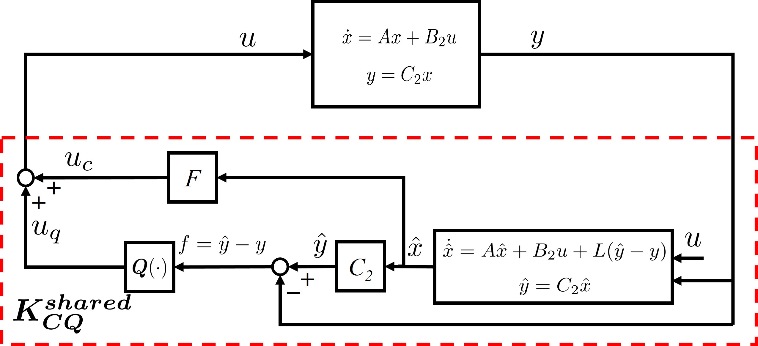
Proposition 2 (Shared Observer)

Given an observer-based state-feedback stabilizing controller 𝐂\bm{C} in (35) with Lo=LL_{o}=L and a separately and arbitrarily designed stabilizing controller 𝐊\bm{K} in (19), then a stable 𝐐{\bm{Q}} in (16) can be realized with

Aq\displaystyle A_{q} =[A+B2DkC2B2CkBkC2Ak],Bq=[LB2DkBk],\displaystyle=\left[\begin{array}[]{cc}A+B_{2}D_{k}C_{2}&B_{2}C_{k}\\ B_{k}C_{2}&A_{k}\end{array}\right],\;B_{q}=\left[\begin{array}[]{c}L-B_{2}D_{k}\\ -B_{k}\end{array}\right], (51)
Cq\displaystyle C_{q} =[DkC2FCk],Dq=Dk,\displaystyle=\left[\begin{array}[]{cc}D_{k}C_{2}-F&C_{k}\end{array}\right],\;D_{q}=-D_{k}, (53)

such that 𝐊𝐂𝐐𝐬𝐡𝐚𝐫𝐞𝐝\bm{K_{CQ}^{shared}} in (46) is stabilizing and 𝐊𝐂𝐐𝐬𝐡𝐚𝐫𝐞𝐝(s)=𝐊(s)\bm{K_{CQ}^{shared}}(s)=\bm{K}(s).

Proof:

The proof is similar to that of Proposition 1 and thus is omitted. In fact, the formulas of (Aq,Bq,Cq,Dq)(A_{q},B_{q},C_{q},D_{q}) can be obtained directly by substituting Ac=A+B2F+LC2A_{c}=A+B_{2}F+LC_{2}, Bc=LB_{c}=-L, Cc=FC_{c}=F, Dc=0D_{c}=0, and Lc=B2L_{c}=-B_{2} into (23), after removing the (stable) uncontrollable mode. ∎

Remark 4

As in Remark 2, 𝐐{\bm{Q}} in (51) can be interpreted as follows. Write xq=[xq,1xq,2]x_{q}=\left[\begin{array}[]{cc}x_{q,1}^{\prime}&x_{q,2}^{\prime}\end{array}\right]^{\prime}, such that 𝐐\bm{Q} can be described as

x˙q,1\displaystyle\dot{x}_{q,1} =(A+B2DkC2)xq,1+B2Ckxq,2+(LB2Dk)f,\displaystyle=(A+B_{2}D_{k}C_{2})x_{q,1}+B_{2}C_{k}x_{q,2}+(L-B_{2}D_{k})f,
x˙q,2\displaystyle\dot{x}_{q,2} =BkC2xq,1+Akxq,2Bkf,\displaystyle=B_{k}C_{2}x_{q,1}+A_{k}x_{q,2}-B_{k}f,
uq\displaystyle u_{q} =(DkC2F)xq,1+Ckxq,2Dkf.\displaystyle=(D_{k}C_{2}-F)x_{q,1}+C_{k}x_{q,2}-D_{k}f.

Likewise, considering u=uku=u_{k} in 𝐊𝐂𝐐𝐬𝐡𝐚𝐫𝐞𝐝\bm{K_{CQ}^{shared}} described by (46), it can be easily checked that

xq,1=x^,xq,2=xk,\displaystyle x_{q,1}=\hat{x},\ \ x_{q,2}=x_{k}, (54)

suggesting that the state of 𝐐{\bm{Q}} corresponds to the states of the Luenberger observer (4) and the controller 𝐊\bm{K}. \Box

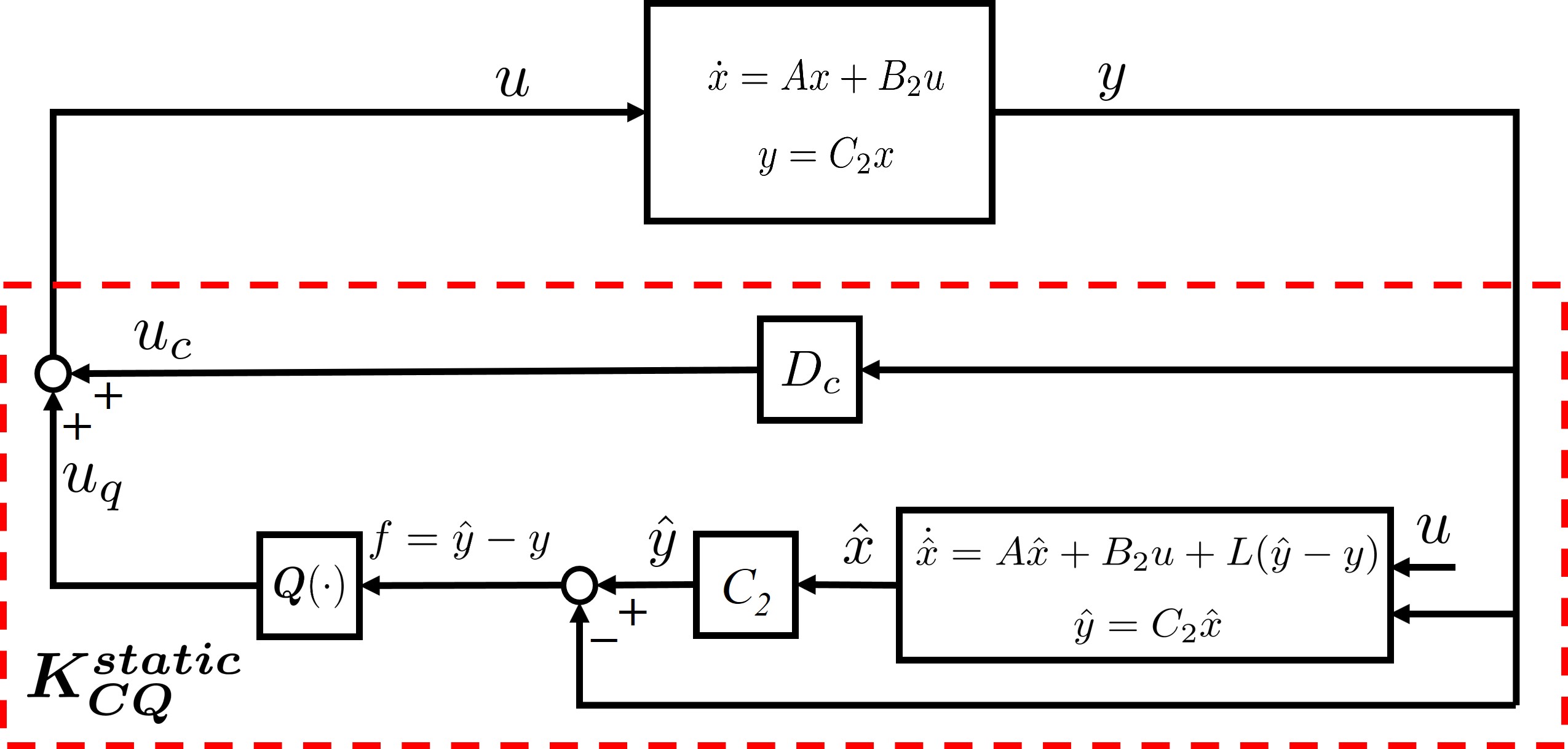
III-B Two-controller structure with static controllers

Assume that there exists a static controller stabilizing system (3). Then let controller 𝑪{\bm{C}} be static:

𝑪:uc=Dcy.\displaystyle{\bm{C}:}u_{c}=D_{c}y. (55)

The controller 𝑲𝑪𝑸\bm{K_{CQ}} in (13) becomes

𝑲𝑪𝑸𝒔𝒕𝒂𝒕𝒊𝒄:{uc=Dcyx^˙=Ax^+B2u+Lfuq=𝑸(f)u=uc+uq.\displaystyle\bm{K_{CQ}^{static}}:\left\{\mspace{-6.0mu}\begin{array}[]{l}u_{c}=D_{c}y\\ \dot{\hat{x}}=A\hat{x}+B_{2}u+Lf\\ u_{q}={\bm{Q}}(f)\\ u=u_{c}+u_{q}.\end{array}\right. (60)

The resulting control system is shown in Fig. 6. The solution to 𝑸{\bm{Q}} in state space is presented in the following proposition and its proof is similar to that of the previous two propositions and thus is omitted.

Proposition 3 (Static Controller)

Given a static stabilizing controller 𝐂\bm{C} in (55) and a separately and arbitrarily designed stabilizing controller 𝐊\bm{K} in (19), then a stable 𝐐{\bm{Q}} in (16) can be realized with

Aq\displaystyle A_{q} =[A+B2DkC2B2CkBkC2Ak],Bq=[LB2DkBk],\displaystyle=\left[\begin{array}[]{cc}A+B_{2}D_{k}C_{2}&B_{2}C_{k}\\ B_{k}C_{2}&A_{k}\end{array}\right],\;B_{q}=\left[\begin{array}[]{c}L-B_{2}D_{k}\\ -B_{k}\end{array}\right], (65)
Cq\displaystyle C_{q} =[(DkDc)C2Ck],Dq=DcDk.\displaystyle=\left[\begin{array}[]{cc}(D_{k}-D_{c})C_{2}&C_{k}\end{array}\right],\;D_{q}=D_{c}-D_{k}. (67)

such that 𝐊𝐂𝐐𝐬𝐭𝐚𝐭𝐢𝐜\bm{K_{CQ}^{static}} in (60) is stabilizing and 𝐊𝐂𝐐𝐬𝐭𝐚𝐭𝐢𝐜(s)=𝐊(s)\bm{K_{CQ}^{static}}(s)=\bm{K}(s).

If controller 𝑲{\bm{K}} is also static, i.e., uk=Dkyu_{k}=D_{k}y, then 𝑸{\bm{Q}} reduces to

Aq\displaystyle A_{q} =A+B2DkC2,Bq=LB2Dk,\displaystyle=A+B_{2}D_{k}C_{2},\;B_{q}=L-B_{2}D_{k},
Cq\displaystyle C_{q} =(DkDc)C2,Dq=DcDk.\displaystyle=(D_{k}-D_{c})C_{2},\;D_{q}=D_{c}-D_{k}. (68)

State feedback: The static state feedback is a special static case when C2=IC_{2}=I. In this case, the observer gain LL can be simply chosen as L=B2DcL=B_{2}D_{c}, as A+LC2=A+B2DcA+LC_{2}=A+B_{2}D_{c} is stable.

Refer to caption
Figure 6: Two-controller structure with static controllers.

IV Multi-Objective Complementary Control (MOCC)

In general, a typical MO control problem specifies different objectives on different channels of the closed-loop system [10, 13, 14, 2, 15, 4, 7]. The objectives under consideration can be roughly divided into two classes: performance involving commands and robustness against unknown disturbances. Performance is meant for transient process, tracking accuracy, passivity requirement [26], etc, while robustness is meant to keep healthy performance in an uncertain or partially unknown environment. It has been pointed out in the Introduction that the traditional design technique using a single controller to address multiple objectives of the closed-loop system usually renders trade-off solutions with compromised performance and robustness in some sense, and for 2DoF controllers there does not exist a general and systematic design method so far to address both performance and the robustness. In contrast, we shall show that MO control problems can be handled effectively by applying the two-controller structures presented in the previous section with two independently designed controllers operating in a naturally complementary way, leading to a MO complementary control (MOCC) framework.

In the sequel, a specific robust tracking control problem is presented to demonstrate the advantages of the proposed MOCC framework. The MO tracking problem under consideration has two objectives: tracking performance and robustness. In the new control structure, 𝑪\bm{C} is designed to address the tracking performance without disturbances, and 𝑲\bm{K} is designed to address the robustness with respect to unknown/uncertain disturbances.

Consider a perturbed FDLTI system (3), described by

{x˙=Ax+B1w+B2uz=C1(C2xr)+D12uy=C2x+D21w,\displaystyle\left\{\mspace{-6.0mu}\begin{array}[]{ll}\dot{x}\mspace{-12.0mu}&=Ax+B_{1}w+B_{2}u\\ z\mspace{-12.0mu}&=C_{1}(C_{2}x-r)+D_{12}u\\ y\mspace{-12.0mu}&=C_{2}x+D_{21}w,\end{array}\right. (72)

where xnx\in\mathbb{R}^{n} is the system state, um2u\in\mathbb{R}^{m_{2}} is the control input, yp2y\in\mathbb{R}^{p_{2}} is the measured output, wm1w\in\mathbb{R}^{m_{1}} is the unknown disturbance input, rp2r\in\mathbb{R}^{p_{2}} known or measurable reference signal, and zp1z\in\mathbb{R}^{p_{1}} consisting of tracking error and control input is an output variable evaluating the tracking performance.

Assume that an admissible tracking controller 𝑪{\bm{C}} is designed as the following form

𝑪:{x˙c=Acxc+Bc(yr)uc=Ccxc+Dc(yr),\displaystyle{\bm{C}}:\left\{\mspace{-6.0mu}\begin{array}[]{l}\dot{x}_{c}=A_{c}x_{c}+B_{c}(y-r)\\ u_{c}=C_{c}x_{c}+D_{c}(y-r),\end{array}\right. (75)

for the system in (72) with w=0w=0, i.e.,

{x˙=Ax+B2uz2=C1(C2xr)+D12uy=C2x,\displaystyle\left\{\mspace{-6.0mu}\begin{array}[]{ll}\dot{x}\mspace{-12.0mu}&=Ax+B_{2}u\\ z_{2}\mspace{-12.0mu}&=C_{1}(C_{2}x-r)+D_{12}u\\ y\mspace{-12.0mu}&=C_{2}x,\end{array}\right. (79)

as shown in Fig. 7.

Refer to caption
Figure 7: Design of the nominal tracking controller 𝑪{\bm{C}}.

On the other hand, assume that a robust controller 𝑲{\bm{K}} having the form of

𝑲:{x˙k=Akxk+Bkyuk=Ckxk+Dky\displaystyle{\bm{K}}:\left\{\mspace{-6.0mu}\begin{array}[]{l}\dot{x}_{k}=A_{k}x_{k}+B_{k}y\\ u_{k}=C_{k}x_{k}+D_{k}y\end{array}\right. (82)

is designed for the system in (72) with r=0r=0, i.e,

{x˙=Ax+B1w+B2uz1=C1C2x+D12uy=C2x+D21w,\displaystyle\left\{\mspace{-6.0mu}\begin{array}[]{ll}\dot{x}\mspace{-12.0mu}&=Ax+B_{1}w+B_{2}u\\ z_{1}\mspace{-12.0mu}&=C_{1}C_{2}x+D_{12}u\\ y\mspace{-12.0mu}&=C_{2}x+D_{21}w,\end{array}\right. (86)

as shown in Fig. 8.

Refer to caption
Figure 8: Design of the robust controller 𝑲{\bm{K}}.

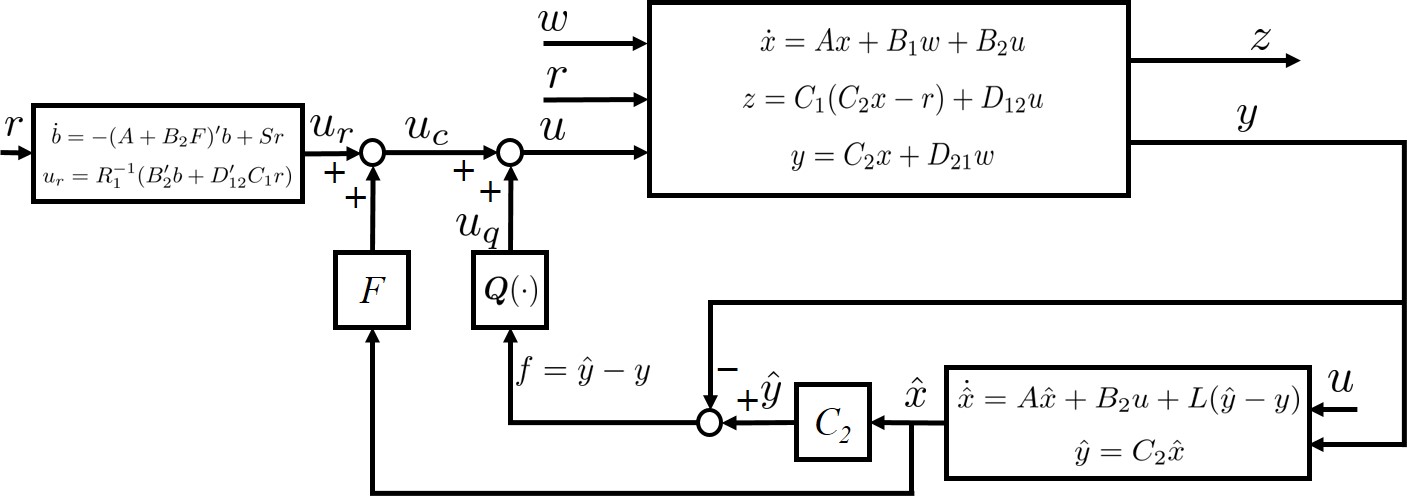
Then by applying the two-controller structure in Fig. 4, a MO tracking controller 𝑲𝑪𝑸𝑻\bm{K_{CQ}^{T}} (the superscript “TT” stands for tracking) can be obtained shown in Fig. 9, where the state-space model of 𝑸\bm{Q} is constructed as that in Proposition 1:

𝑸:{x˙q=Aqxq+Bqfuq=Cqxq+Dqf,\displaystyle{\bm{Q}}:\left\{\mspace{-6.0mu}\begin{array}[]{l}\dot{x}_{q}=A_{q}x_{q}+B_{q}f\\ u_{q}=C_{q}x_{q}+D_{q}f,\end{array}\right.

with (Aq,Bq,Cq,Dq)(A_{q},B_{q},C_{q},D_{q}) given by (23). Note that the difference between the controller 𝑲𝑪𝑸\bm{K_{CQ}} in Fig. 4 and the tracking controller 𝑲𝑪𝑸𝑻\bm{K_{CQ}^{T}} in Fig. 9 is that for 𝑲𝑪𝑸𝑻\bm{K_{CQ}^{T}}, the reference signal rr is also as an input to generate the control signal ucu_{c}. Then it follows from Proposition 1 that for the tracking control system with 𝑲𝑪𝑸𝑻\bm{K_{CQ}^{T}}, the transfer matrix from yy to uu is 𝑲(s)\bm{K}(s).

Refer to caption
Figure 9: MO tracking control system by two-controller structure.
Remark 5

As the two-controller structure studied in Section III, the tracking controller 𝐊𝐂𝐐𝐓\bm{K_{CQ}^{T}} can also have shared-observer and static structures. If the tracking controller 𝐂\bm{C} in (75) is observer-based with Ac=A+B2F+LC2A_{c}=A+B_{2}F+LC_{2}, Bc=LB_{c}=-L, Cc=FC_{c}=F, Dc=0D_{c}=0, and Lc=B2L_{c}=-B_{2}, then ucu_{c} in 𝐊𝐂𝐐𝐓\bm{K_{CQ}^{T}} becomes

uc=Fxc,x˙c=Axc+B2u+L(C2xcy+r).\displaystyle u_{c}=Fx_{c},\;\dot{x}_{c}=Ax_{c}+B_{2}u+L(C_{2}x_{c}-y+r).

Write xcx_{c} above as a sum of two terms: xc=x~c+xrx_{c}=\tilde{x}_{c}+x_{r}, such that

x~˙c\displaystyle\dot{\tilde{x}}_{c} =Ax~c+B2u+L(C2x~cy),\displaystyle=A\tilde{x}_{c}+B_{2}u+L(C_{2}\tilde{x}_{c}-y),
x˙r\displaystyle\dot{x}_{r} =(A+LC2)xr+Lr.\displaystyle=(A+LC_{2})x_{r}+Lr.

Then similar to the controller 𝐊𝐂𝐐𝐬𝐡𝐚𝐫𝐞𝐝\bm{K_{CQ}^{shared}} in (46), the tracking controller 𝐊𝐂𝐐𝐓\bm{K_{CQ}^{T}} with shared observer is described as

𝑲𝑪𝑸𝒔𝒉𝒂𝒓𝒆𝒅,𝑻:{x^˙=Ax^+B2u+Lfx˙r=(A+LC2)xr+Lruc=F(x^+xr)uq=𝑸(f)u=uc+uq.\displaystyle\bm{K_{CQ}^{shared,T}}:\left\{\mspace{-6.0mu}\begin{array}[]{l}\dot{\hat{x}}=A\hat{x}+B_{2}u+Lf\\ \dot{x}_{r}=(A+LC_{2})x_{r}+Lr\\ u_{c}=F(\hat{x}+x_{r})\\ u_{q}={\bm{Q}}(f)\\ u=u_{c}+u_{q}.\end{array}\right.

The parameters (Aq,Bq,Cq,Dq)(A_{q},B_{q},C_{q},D_{q}) of 𝐐\bm{Q} are given by Proposition 2. If the tracking controller 𝐂\bm{C} in (75) is static as uc=Dc(yr)u_{c}=D_{c}(y-r), the tracking controller 𝐊𝐂𝐐𝐓\bm{K_{CQ}^{T}} is simply given by

𝑲𝑪𝑸𝒔𝒕𝒂𝒕𝒊𝒄,𝑻:{uc=Dc(yr)x^˙=Ax^+B2u+Lfuq=𝑸(f)u=uc+uq\displaystyle\bm{K_{CQ}^{static,T}}:\left\{\mspace{-6.0mu}\begin{array}[]{l}u_{c}=D_{c}(y-r)\\ \dot{\hat{x}}=A\hat{x}+B_{2}u+Lf\\ u_{q}={\bm{Q}}(f)\\ u=u_{c}+u_{q}\end{array}\right.

with (Aq,Bq,Cq,Dq)(A_{q},B_{q},C_{q},D_{q}) given by Proposition 3. \Box

Next, we shall conduct a performance analysis for the resulting tracking controller 𝑲𝑪𝑸𝑻\bm{K_{CQ}^{T}}. It will be shown that the tracking controller 𝑲𝑪𝑸𝑻\bm{K_{CQ}^{T}} consisting of 𝑪{\bm{C}} for the nominal tracking performance and 𝑲{\bm{K}} for the robustness leads to a decoupled design and the two controllers 𝑪{\bm{C}} and 𝑲{\bm{K}} operate in a complementary way.

IV-A Performance analysis

In principle, the objective of performance analysis in this paper is to determine the closed-loop performance generated by 𝑲𝑪𝑸𝑻\bm{K_{CQ}^{T}} under certain specified criteria such as the L1L_{1} norm and L2L_{2} norm of zz. Here, we shall choose the power norm of bounded power signals, since it can be used for persistent signals and is related to the quadratic criterion and the \mathcal{H}_{\infty} norm. It is common to use the power norm of bounded power signals in the analysis of control systems, e.g. [13, 14, 4, 27, 28]. All signals considered in this paper are assumed to be deterministic. In the sequel, the notion of bounded power signals is introduced.

Given a real vector signal u(t)u(t) that is zero for t<0t<0, its asymptotically stationary autocorrelation matrix is defined as

Ruu(τ)=limT1T0Tu(t+τ)u(t)dt.\displaystyle R_{uu}(\tau)=\lim\limits_{T\to\infty}\frac{1}{T}\int_{0}^{T}u(t+\tau)u(t)^{\prime}{\rm d}t.

The Fourier transform of Ruu(τ)R_{uu}(\tau) called the (power) spectral density of uu, if exists, is

𝑺𝒖𝒖(jω):=Ruu(τ)ejωτdτ.\displaystyle\bm{S_{uu}}(j\omega):=\int_{-\infty}^{\infty}R_{uu}(\tau)e^{-j\omega\tau}{\rm d}\tau.

Then the bounded power signals are defined as follows.

Definition 1 ([13])

A signal uu is said to have bounded power if it satisfies the following conditions:

  • 1.

    u(t)\|u(t)\| is bounded for all t0t\geq 0;

  • 2.

    The autocorrelation matrix Ruu(τ)R_{uu}(\tau) exists for all τ\tau and the spectral density matrix 𝑺𝒖𝒖(jω)\bm{S_{uu}}(j\omega) exists;

  • 3.

    limT1T0Tu(t)2dt<\lim\limits_{T\to\infty}\frac{1}{T}\int_{0}^{T}\|u(t)\|^{2}{\rm d}t<\infty.

The set of all signals having bounded power is denoted by 𝒫\mathcal{P}. A seminorm can be defined on 𝒫\mathcal{P}:

u𝒫\displaystyle\|u\|_{\mathcal{P}} =limT1T0Tu(t)2dt\displaystyle=\sqrt{\lim\limits_{T\to\infty}\frac{1}{T}\int_{0}^{T}\|u(t)\|^{2}{\rm d}t}
=Trace[Ruu(0)]u𝒫.\displaystyle=\sqrt{{\rm Trace}[R_{uu}(0)]}\;\;\forall u\in\mathcal{P}. (89)

The power seminorm of a signal can also be computed from its spectral density matrix by using the inverse Fourier transform of Ruu(τ)R_{uu}(\tau):

u𝒫=12πTrace[𝑺𝒖𝒖(jω)]dω=𝒖(s)𝒫,\displaystyle\|u\|_{\mathcal{P}}=\sqrt{\frac{1}{2\pi}\int_{-\infty}^{\infty}{\rm Trace}[\bm{S_{uu}}(j\omega)]{\rm d}\omega}=\|\bm{u}(s)\|_{\cal P}, (90)

which is derived from the Parseval theorem in the average power case [29, Section 3.5.7] with 𝒖(s)\bm{u}(s) being the Laplace transform of u(t)u(t). The cross-correlation between two real signals uu and vv is defined as

Ruv(τ)=limT1T0Tu(t+τ)v(t)dt,\displaystyle R_{uv}(\tau)=\lim\limits_{T\to\infty}\frac{1}{T}\int_{0}^{T}u(t+\tau)v(t)^{\prime}{\rm d}t,

and its Fourier transform is denoted by 𝑺𝒖𝒗(jω)\bm{S_{uv}}(j\omega), called cross (power) spectral density.

Now consider the tracking control system in Fig. 9, with 𝑸\bm{Q} constructed according to Proposition 1. Both the disturbance signal ww and the reference signal rr are assumed to be bounded power signals, i.e., w,r𝒫w,r\in\mathcal{P}. The closed-loop performance will be measured in terms of the power norm of the performance output zz, i.e., z𝒫\|z\|_{\mathcal{P}}. First, the closed-loop system can be described by

𝑻:{x¯˙=A¯x¯+B¯1w+B¯rrz=C¯1x¯+Drr,\displaystyle\bm{T}:\left\{\mspace{-6.0mu}\begin{array}[]{l}\dot{\bar{x}}=\bar{A}\bar{x}+\bar{B}_{1}w+\bar{B}_{r}r\\ z=\bar{C}_{1}\bar{x}+D_{r}r,\end{array}\right. (93)

where x¯:=[xxx^xcxq]{\bar{x}}:=\left[\begin{array}[]{cccc}x^{\prime}&x^{\prime}-\hat{x}^{\prime}&x_{c}^{\prime}&x_{q}^{\prime}\end{array}\right]^{\prime} and

A¯\displaystyle\bar{A} =[A+B2DcC2B2DqC2B2CcB2Cq0A+LC200BcC2LcDqC2AcLcCq0BqC20Aq],\displaystyle=\left[\begin{array}[]{cccc}A+B_{2}D_{c}C_{2}&-B_{2}D_{q}C_{2}&B_{2}C_{c}&B_{2}C_{q}\\ 0&A+LC_{2}&0&0\\ B_{c}C_{2}&L_{c}D_{q}C_{2}&A_{c}&-L_{c}C_{q}\\ 0&-B_{q}C_{2}&0&A_{q}\\ \end{array}\right],
B¯1\displaystyle\bar{B}_{1} =[B1+B2(DcDq)D21B1+LD21(Bc+LcDq)D21BqD21],B¯r=[B2Dc0Bc0],\displaystyle=\left[\begin{array}[]{c}B_{1}+B_{2}(D_{c}-D_{q})D_{21}\\ B_{1}+LD_{21}\\ (B_{c}+L_{c}D_{q})D_{21}\\ -B_{q}D_{21}\end{array}\right],\;\bar{B}_{r}=\left[\begin{array}[]{c}-B_{2}D_{c}\\ 0\\ -B_{c}\\ 0\end{array}\right],
C¯1\displaystyle\bar{C}_{1} =[(C1+D12Dc)C2D12DqC2D12CcD12Cq],\displaystyle=\left[\mspace{-6.0mu}\begin{array}[]{ccccc}(C_{1}+D_{12}D_{c})C_{2}&-D_{12}D_{q}C_{2}&D_{12}C_{c}&D_{12}C_{q}\end{array}\mspace{-6.0mu}\right],
Dr\displaystyle D_{r} =(C1+D12Dc).\displaystyle=-(C_{1}+D_{12}D_{c}).

The following decoupled result is important in this paper, which characterizes the nature of the closed-loop system with the controller 𝑲𝑪𝑸𝑻\bm{K_{CQ}^{T}}.

𝑻(s)\displaystyle\bm{T}(s) =[𝒜1r𝒞1D1Dr]\displaystyle=\left[\begin{array}[]{c|cc}\mathcal{A}&\mathcal{B}_{1}&\mathcal{B}_{r}\\ \hline\cr\mathcal{C}_{1}&D_{1}&D_{r}\end{array}\right] (30)
=\displaystyle= [A+B2DcC20B2Cc0000B2Dc0A+LC20000B1+LD210BcC20Ac0000Bc000Ac+LcCc(Bc+LcDq)C2LcCk(Bc+LcDq)D2100000A+B2DkC2B2CkB1+B2DkD2100000BkC2AkBkD210(C1+D12Dc)C20D12Cc0(C1+D12Dk)C2D12Ck0Dr].\displaystyle\left[\begin{array}[]{cccccc|cc}A+B_{2}D_{c}C_{2}&0&B_{2}C_{c}&0&0&0&0&-B_{2}D_{c}\\ 0&A+LC_{2}&0&0&0&0&B_{1}+LD_{21}&0\\ B_{c}C_{2}&0&A_{c}&0&0&0&0&-B_{c}\\ 0&0&0&A_{c}+L_{c}C_{c}&(B_{c}+L_{c}D_{q})C_{2}&-L_{c}C_{k}&(B_{c}+L_{c}D_{q})D_{21}&0\\ 0&0&0&0&A+B_{2}D_{k}C_{2}&B_{2}C_{k}&B_{1}+B_{2}D_{k}D_{21}&0\\ 0&0&0&0&B_{k}C_{2}&A_{k}&B_{k}D_{21}&0\\ \hline\cr(C_{1}+D_{12}D_{c})C_{2}&0&D_{12}C_{c}&0&(C_{1}+D_{12}D_{k})C_{2}&D_{12}C_{k}&0&D_{r}\end{array}\right]. (38)

Lemma 1

The closed-loop system (93) can be represented as the following form of transfer matrix in terms of state-space matrices:

𝑻(s)\displaystyle\bm{T}(s) =[A¯B¯1B¯rC¯10Dr]=[𝑻𝒛𝟏𝒘(s)𝑻𝒛𝟐𝒓(s)],\displaystyle=\left[\begin{array}[]{c|cc}\bar{A}&\bar{B}_{1}&\bar{B}_{r}\\ \hline\cr\bar{C}_{1}&0&D_{r}\end{array}\right]=\left[\begin{array}[]{cc}\bm{T_{z_{1}w}}(s)&\bm{T_{z_{2}r}}(s)\end{array}\right], (97)

where

𝑻𝒛𝟏𝒘(s)\displaystyle\bm{T_{z_{1}w}}(s)\mspace{-6.0mu} =[A+B2DkC2B2CkB1+B2DkD21BkC2AkBkD21(C1+D12Dk)C2D12Ck0]\displaystyle=\mspace{-6.0mu}\left[\mspace{-6.0mu}\begin{array}[]{cc|c}A+B_{2}D_{k}C_{2}&B_{2}C_{k}&B_{1}+B_{2}D_{k}D_{21}\\ B_{k}C_{2}&A_{k}&B_{k}D_{21}\\ \hline\cr(C_{1}+D_{12}D_{k})C_{2}&D_{12}C_{k}&0\end{array}\mspace{-6.0mu}\right]
𝑻𝒛𝟐𝒓(s)\displaystyle\bm{T_{z_{2}r}}(s)\mspace{-6.0mu} =[A+B2DcC2B2CcB2DcBcC2AcBc(C1+D12Dc)C2D12Cc(C1+D12Dc)],\displaystyle=\mspace{-6.0mu}\left[\mspace{-6.0mu}\begin{array}[]{cc|c}A+B_{2}D_{c}C_{2}&B_{2}C_{c}&-B_{2}D_{c}\\ B_{c}C_{2}&A_{c}&-B_{c}\\ \hline\cr(C_{1}+D_{12}D_{c})C_{2}&D_{12}C_{c}&-(C_{1}+D_{12}D_{c})\end{array}\mspace{-6.0mu}\right],

with z1z_{1} and z2z_{2} defined in (86) and (79), respectively.

Proof:

Substituting the formulas of Aq,Bq,Cq,DqA_{q},B_{q},C_{q},D_{q} in (23) into the closed-loop system (93) and using the linear transformation χ=Xx¯\chi=X\bar{x} with

X=[II00I00I000000II00000I000I00I000000I],\displaystyle X=\left[\begin{array}[]{cccccc}I&-I&0&0&-I&0\\ 0&I&0&0&0&0\\ 0&0&I&-I&0&0\\ 0&0&0&I&0&0\\ 0&I&0&0&I&0\\ 0&0&0&0&0&I\end{array}\right],

we have

𝑻(s)\displaystyle\bm{T}(s) =[𝒜1r𝒞10Dr],\displaystyle=\left[\begin{array}[]{c|cc}\mathcal{A}&\mathcal{B}_{1}&\mathcal{B}_{r}\\ \hline\cr\mathcal{C}_{1}&0&D_{r}\end{array}\right],

where 𝒜=XA¯X1,1=XB¯1,r=XB¯r,𝒞1=C¯1X1\mathcal{A}=X\bar{A}X^{-1},\mathcal{B}_{1}=X\bar{B}_{1},\mathcal{B}_{r}=X\bar{B}_{r},\mathcal{C}_{1}=\bar{C}_{1}X^{-1} and their detailed expressions are shown in (30) in the bottom of the next page. Then, it can be readily obtained the state-space data of 𝑻𝒛𝟏𝒘(s)\bm{T_{z_{1}w}}(s) and 𝑻𝒛𝟐𝒓(s)\bm{T_{z_{2}r}}(s) in the theorem. ∎

It is clearly seen that the closed-loop transfer function 𝑻(s){\bm{T}}(s) consists of 𝑻𝒛𝟏𝒘(s)\bm{T_{z_{1}w}}(s) and 𝑻𝒛𝟐𝒓(s)\bm{T_{z_{2}r}}(s) which depend on the controller 𝑲{\bm{K}} and the controller 𝑪{\bm{C}} separately, and 𝑻(s)\bm{T}(s) does not depend on LL and LcL_{c}. Note that 𝑻𝒛𝟏𝒘(s)\bm{T_{z_{1}w}}(s) and 𝑻𝒛𝟐𝒓(s)\bm{T_{z_{2}r}}(s) are the closed-loop transfer matrices in Figs. 8 and 7, respectively. The total performance achieved by 𝑲\bm{K} and 𝑪\bm{C} is characterized in the analysis below, through the power norm of zz. Due to the neat separate transfer matrices 𝑻𝒛𝟏𝒘(s)\bm{T_{z_{1}w}}(s) and 𝑻𝒛𝟐𝒓(s)\bm{T_{z_{2}r}}(s), we shall analyze z𝒫\|z\|_{\mathcal{P}} in the frequency domain.

Defining v:=[wr]v:=\left[\begin{array}[]{cc}w\\ r\end{array}\right], then the spectral density matrix of vv can be written as

𝑺𝒗𝒗(jω)=[𝑺𝒘𝒘(jω)𝑺𝒘𝒓(jω)𝑺𝒘𝒓(jω)𝑺𝒓𝒓(jω)].\displaystyle\bm{S_{vv}}(j\omega)=\left[\begin{array}[]{cc}\bm{S_{ww}}(j\omega)&\bm{S_{wr}}(j\omega)\\ \bm{S_{wr}^{*}}(j\omega)&\bm{S_{rr}}(j\omega)\end{array}\right].

From the spectral analysis [13] and (90), we get

𝑺𝒛𝒛=[𝑻𝒛𝟏𝒘𝑻𝒛𝟐𝒓][𝑺𝒘𝒘𝑺𝒘𝒓𝑺𝒘𝒓𝑺𝒓𝒓][𝑻𝒛𝟏𝒘𝑻𝒛𝟐𝒓]\displaystyle\bm{S_{zz}}=\left[\begin{array}[]{cc}\bm{T_{z_{1}w}}&\bm{T_{z_{2}r}}\end{array}\right]\left[\begin{array}[]{cc}\bm{S_{ww}}&\bm{S_{wr}}\\ \bm{S_{wr}^{*}}&\bm{S_{rr}}\end{array}\right]\left[\begin{array}[]{c}\bm{T_{z_{1}w}^{*}}\\ \bm{T_{z_{2}r}^{*}}\end{array}\right] (104)

and

z𝒫=12πTrace[𝑺𝒛𝒛(jω)]dω.\displaystyle\|z\|_{\mathcal{P}}=\sqrt{\frac{1}{2\pi}\int_{-\infty}^{\infty}{\rm Trace}[\bm{S_{zz}}(j\omega)]{\rm d}\omega}. (105)

Generally, the disturbance signal ww and the reference signal rr could be independent or dependent on each other. Signals ww and rr are said to be orthogonal or independent if 𝑺𝒘𝒓=0\bm{S_{wr}}=0 [30, 13]. For example, any two sinusoidal signals uu and vv with different frequencies are orthogonal since the cross-correlation matrix Ruv(τ)=0,τR_{uv}(\tau)=0,\forall\tau which is the orthogonal case. The dependent case could happen when ww is induced by plant parameter uncertainties, which in turn is related to the reference signal rr in some way. Performance evaluations are carried out for both orthogonal and dependent cases and summarized in the following two theorems.

Theorem 1

Let ww and rr be orthogonal, that is, 𝐒𝐰𝐫=0\bm{S_{wr}}=0. Given any controllers 𝐂\bm{C} and 𝐊\bm{K} in (75) and (82), then the performance measure z𝒫2\|z\|_{\mathcal{P}}^{2} for the closed-loop system (93) is sum of two separate terms:

z𝒫2\displaystyle\|z\|_{\mathcal{P}}^{2} =z1𝒫2+z2𝒫2,\displaystyle=\|z_{1}\|_{\mathcal{P}}^{2}+\|z_{2}\|_{\mathcal{P}}^{2}, (106)

where

z1𝒫2\displaystyle\|z_{1}\|_{\mathcal{P}}^{2} =12πTrace[𝑻𝒛𝟏𝒘(jω)𝑺𝒘𝒘(jω)𝑻𝒛𝟏𝒘(jω)]dω,\displaystyle=\frac{1}{2\pi}\int_{-\infty}^{\infty}{\rm Trace}[\bm{T_{z_{1}w}}(j\omega)\bm{S_{ww}}(j\omega)\bm{T_{z_{1}w}}^{*}(j\omega)]{\rm d}\omega,
z2𝒫2\displaystyle\|z_{2}\|_{\mathcal{P}}^{2} =12πTrace[𝑻𝒛𝟐𝒓(jω)𝑺𝒓𝒓(jω)𝑻𝒛𝟐𝒓(jω)]dω,\displaystyle=\frac{1}{2\pi}\int_{-\infty}^{\infty}{\rm Trace}[\bm{T_{z_{2}r}}(j\omega)\bm{S_{rr}}(j\omega)\bm{T_{z_{2}r}^{*}}(j\omega)]{\rm d}\omega,

with 𝐓𝐳𝟏𝐰(s)\bm{T_{z_{1}w}}(s) and 𝐓𝐳𝟐𝐫(s)\bm{T_{z_{2}r}}(s) dependent on 𝐊{\bm{K}} and 𝐂{\bm{C}} respectively according to Lemma 1.

Proof:

The proof can be done by direct calculation. Since 𝒛=𝑻𝒛𝟏𝒘𝟏𝒘+𝑻𝒛𝟐𝒓𝒓\bm{z}=\bm{T_{z_{1}w_{1}}}\bm{w}+\bm{T_{z_{2}r}}\bm{r}, if ww and rr are orthogonal, i.e., 𝑺𝒘𝒓=0\bm{S_{wr}}=0, recalling 𝑺𝒛𝒛(jω)\bm{S_{zz}}(j\omega) and z𝒫\|z\|_{\mathcal{P}} given in (104) and (105), we immediately have

z𝒫2=\displaystyle\|z\|_{\mathcal{P}}^{2}= 12πTrace[𝑺𝒛𝒛(jω)]dω\displaystyle\frac{1}{2\pi}\int_{-\infty}^{\infty}{\rm Trace}[\bm{S_{zz}}(j\omega)]{\rm d}\omega
=\displaystyle= 12π(Trace[𝑻𝒛𝟏𝒘(jω)𝑺𝒘𝒘(jω)𝑻𝒛𝟏𝒘(jω)]\displaystyle\frac{1}{2\pi}\int_{-\infty}^{\infty}\Big{(}{\rm Trace}[\bm{T_{z_{1}w}}(j\omega)\bm{S_{ww}}(j\omega)\bm{T_{z_{1}w}^{*}}(j\omega)]
+Trace[𝑻𝒛𝟐𝒓(jω)𝑺𝒓𝒓(jω)𝑻𝒛𝟐𝒓(jω)])dω,\displaystyle+{\rm Trace}[\bm{T_{z_{2}r}}(j\omega)\bm{S_{rr}}(j\omega)\bm{T_{z_{2}r}^{*}}(j\omega)]\Big{)}{\rm d}\omega,
=\displaystyle= z1𝒫2+z2𝒫2,\displaystyle\|z_{1}\|_{\mathcal{P}}^{2}+\|z_{2}\|_{\mathcal{P}}^{2},

where z2𝒫2=12πTrace[𝑻𝒛𝟐𝒓(jω)𝑺𝒓𝒓(jω)𝑻𝒛𝟐𝒓(jω)]dω\|z_{2}\|_{\mathcal{P}}^{2}=\frac{1}{2\pi}\int_{-\infty}^{\infty}{\rm Trace}[\bm{T_{z_{2}r}}(j\omega)\bm{S_{rr}}(j\omega)\bm{T_{z_{2}r}^{*}}(j\omega)]{\rm d}\omega and z1𝒫2=12πTrace[𝑻𝒛𝟏𝒘(jω)𝑺𝒘𝒘(jω)𝑻𝒛𝟏𝒘(jω)]dω\|z_{1}\|_{\mathcal{P}}^{2}=\frac{1}{2\pi}\int_{-\infty}^{\infty}{\rm Trace}[\bm{T_{z_{1}w}}(j\omega)\bm{S_{ww}}(j\omega)\bm{T_{z_{1}w}}^{*}(j\omega)]{\rm d}\omega. ∎

Remark 6

It is clear that the nominal tracking performance is characterized in z2𝒫\|z_{2}\|_{\cal P} with respect to the reference signal rr and the impact of disturbance ww (hence, the robustness) is measured in z1𝒫\|z_{1}\|_{\cal P}. Since 𝐓𝐳𝟏𝐰\bm{T_{z_{1}w}} only depends on 𝐊\bm{K} and 𝐓𝐳𝟐𝐫\bm{T_{z_{2}r}} is only related to 𝐂\bm{C}, Theorem 1 shows that if ww and rr are orthogonal, there is no trade-off between the design of 𝐂{\bm{C}} for the nominal tracking performance z2𝒫\|z_{2}\|_{\cal P} and the design of 𝐊{\bm{K}} for the robustness. In other words, the two independently designed controllers 𝐂{\bm{C}} and 𝐊{\bm{K}} operate in a naturally complementary way, and, obviously, when w=0w=0, the nominal tracking performance can be fully kept by 𝐂\bm{C}. Furthermore, it can also be seen that, to achieve better robust tracking performance, 𝐂\bm{C} should be designed to bring z2𝒫\|z_{2}\|_{\cal P} low, while 𝐊\bm{K} can be designed to be a robust controller. For example, if 𝐊\bm{K} is designed to be an {\cal H}_{\infty} control for a given γ>0\gamma>0, then z1𝒫<γw𝒫\|z_{1}\|_{\cal P}<\gamma\|w\|_{\cal P}. In general, for a given 𝐊\bm{K}, z1𝒫𝐓𝐳𝟏𝐰(s)w𝒫\|z_{1}\|_{\cal P}\leq\|\bm{T_{z_{1}w}}(s)\|_{\infty}\|w\|_{\cal P}. In this sense, the operator 𝐐\bm{Q} obtained in Proposition 1 achieves the two objectives of nominal tracking performance and minimization of 𝐓𝐳𝟏𝐰(s)\|\bm{T_{z_{1}w}}(s)\|_{\infty} simultaneously. \Box

Remark 7

It is also noted that the controller 𝐂\bm{C} could itself be designed to address multiple optimal performance objectives such as the controller in Lemma 1 of [31] that is derived from the Youla parameter to optimize multiple costs simultaneously. Since no impact of uncertain disturbance is counted, this controller could be complemented by the 𝐐\bm{Q} constructed in the MOCC design of this paper to achieve non-compromised robust optimal performance with respect to uncertain disturbance. \Box

The performance analysis for the dependent case could be more complicated due to the complexity of dependency between ww and rr. In this paper, performance analysis is done for the case that w=𝑾(r)+w1w=\bm{W}(r)+w_{1}, where 𝑾()\bm{W}(\cdot) is assumed to be a mapping satisfying 𝑾(r)𝒫<,𝑾(0)=0,r𝒫\|\bm{W}(r)\|_{\cal P}<\infty,\;\bm{W}(0)=0,\;\forall r\in{\cal P}, and w1𝒫w_{1}\in\mathcal{P} is the orthogonal part of ww with both rr and 𝑾(r)\bm{W}(r), i.e., 𝑺𝒘𝟏𝒓=0\bm{S_{w_{1}r}}=0 and 𝑺𝒘𝟏𝑾(𝒓)=0\bm{S_{w_{1}\bm{W}(r)}}=0. The system in (72) then becomes

{x˙=Ax+B1(𝑾(r)+w1)+B2uz=C1(C2xr)+D12uy=C2x+D21(𝑾(r)+w1).\displaystyle\left\{\mspace{-6.0mu}\begin{array}[]{ll}\dot{x}\mspace{-12.0mu}&=Ax+B_{1}(\bm{W}(r)+w_{1})+B_{2}u\\ z\mspace{-12.0mu}&=C_{1}(C_{2}x-r)+D_{12}u\\ y\mspace{-12.0mu}&=C_{2}x+D_{21}(\bm{W}(r)+w_{1}).\end{array}\right. (110)

The MO tracking control system in Fig. 9 can be modified as Fig. 10.

Refer to caption
Figure 10: MO tracking control system by two-controller structure in the dependent case.

For a linear time-invariant mapping 𝑾(r)\bm{W}(r), denoting the Laplace transform of 𝑾(r)\bm{W}(r) as 𝑾𝒓(s)\bm{W_{r}}(s), then

𝑾(r)𝒫\displaystyle\|\bm{W}(r)\|_{\cal P} =12πTrace[𝑺𝑾(𝒓)𝑾(𝒓)(jω)]dω\displaystyle=\sqrt{\frac{1}{2\pi}\int_{-\infty}^{\infty}{\rm Trace}\left[\bm{S_{\bm{W}(r)\bm{W}(r)}}(j\omega)\right]{\rm d}\omega}
=𝑾𝒓(s)𝒫,\displaystyle=\|\bm{W_{r}}(s)\|_{\cal P},

and 𝒘(s)=𝑾𝒓(s)+𝒘1(s)\bm{w}(s)=\bm{W_{r}}(s)+\bm{w}_{1}(s). Now we are ready to present the following performance analysis result in the dependent case.

Theorem 2

For dependent ww and rr as in w=𝐖(r)+w1w=\bm{W}(r)+w_{1}, where 𝐖(r)\bm{W}(r) is an LTI mapping with 𝐖r(s)=𝐖(s)𝐫(s),𝐖(s)\bm{W}_{r}(s)=\bm{W}(s)\bm{r}(s),\bm{W}(s)\in\mathcal{RL}_{\infty}, and w1w_{1} is orthogonal of both rr and 𝐖(r)\bm{W}(r) in the sense that 𝐒𝐰𝟏𝐫=0\bm{S_{w_{1}r}}=0 and 𝐒𝐰𝟏𝐖(𝐫)=0\bm{S_{w_{1}\bm{W}(r)}}=0, given any controllers 𝐂\bm{C} and 𝐊\bm{K} in (75) and (82), the following equations hold:

z𝒫2=\displaystyle\|z\|_{\mathcal{P}}^{2}= z1𝒫2+z~2𝒫2,\displaystyle\|z_{1}\|_{\mathcal{P}}^{2}+\|\tilde{z}_{2}\|_{\mathcal{P}}^{2}, (111)
z𝒫2γ2w𝒫2=\displaystyle\|z\|_{\mathcal{P}}^{2}-\gamma^{2}\|w\|_{\mathcal{P}}^{2}= z1𝒫2γ2w1𝒫2\displaystyle\|z_{1}\|_{\mathcal{P}}^{2}-\gamma^{2}\|w_{1}\|_{\mathcal{P}}^{2}
+z~2𝒫2γ2𝑾(r)𝒫2,\displaystyle~{}~{}~{}~{}+\|\tilde{z}_{2}\|_{\mathcal{P}}^{2}-\gamma^{2}\|\bm{W}(r)\|_{\mathcal{P}}^{2}, (112)

where γ\gamma is a scalar level constant,

z1𝒫2\displaystyle\|z_{1}\|_{\mathcal{P}}^{2} =12πTrace[𝑻𝒛𝟏𝒘(jω)𝑺𝒘𝟏𝒘𝟏(jω)𝑻𝒛𝟏𝒘(jω)]dω\displaystyle=\frac{1}{2\pi}\int_{-\infty}^{\infty}{\rm Trace}[\bm{T_{z_{1}w}}(j\omega)\bm{S_{w_{1}w_{1}}}(j\omega)\bm{T_{z_{1}w}}^{*}(j\omega)]{\rm d}\omega
𝒛~𝟐(s)\displaystyle\bm{\tilde{z}_{2}}(s) =𝑻𝒛𝟏𝒘(s)𝑾𝒓(s)+𝑻𝒛𝟐𝒓(s)𝒓(s)\displaystyle=\bm{T_{z_{1}w}}(s)\bm{W_{r}}(s)+\bm{T_{z_{2}r}}(s)\bm{r}(s)
=𝑻𝒛𝟏𝒘(s)𝑾𝒓(s)+𝒛𝟐(s)\displaystyle=\bm{T_{z_{1}w}}(s)\bm{W_{r}}(s)+\bm{z_{2}}(s)
z2𝒫2\displaystyle\|z_{2}\|_{\mathcal{P}}^{2} =12πTrace[𝑻𝒛𝟐𝒓(jω)𝑺𝒓𝒓(jω)𝑻𝒛𝟐𝒓(jω)]dω,\displaystyle=\frac{1}{2\pi}\int_{-\infty}^{\infty}{\rm Trace}[\bm{T_{z_{2}r}}(j\omega)\bm{S_{rr}}(j\omega)\bm{T_{z_{2}r}^{*}}(j\omega)]{\rm d}\omega,

and 𝐓𝐳𝟏𝐰(s)\bm{T_{z_{1}w}}(s) and 𝐓𝐳𝟐𝐫(s)\bm{T_{z_{2}r}}(s) are derived in Lemma 1. Moreover, if 𝐊\bm{K} is designed to be an {\cal H}_{\infty} control for a given γ>0\gamma>0 such that 𝐓𝐳𝟏𝐰<γ\|\bm{T_{z_{1}w}}\|_{\infty}<\gamma, then, regardless of 𝐂\bm{C}, we have

sup𝑾(𝒔){z~2𝒫2γ2𝑾(s)𝒓(s)𝒫2}\displaystyle\sup_{\bm{W(s)}\in\mathcal{RL}_{\infty}}\left\{\|\tilde{z}_{2}\|_{\mathcal{P}}^{2}-\gamma^{2}\|\bm{W}(s)\bm{r}(s)\|_{\mathcal{P}}^{2}\right\}
=\displaystyle= z~2𝒫2γ2𝑾~𝒓(s)𝒫2\displaystyle\|\tilde{z}_{2}\|_{\mathcal{P}}^{2}-\gamma^{2}\|\bm{\widetilde{W}}\bm{r}(s)\|_{\mathcal{P}}^{2}
=\displaystyle= 12πTrace[𝑺𝒓𝒓𝑻𝒛𝟐𝒓(Iγ2𝑻𝒛𝟏𝒘𝑻𝒛𝟏𝒘)1𝑻𝒛𝟐𝒓]dω,\displaystyle\frac{1}{2\pi}\int_{-\infty}^{\infty}{\rm Trace}\big{[}\bm{S_{rr}}\bm{T_{z_{2}r}}^{*}(I-\gamma^{-2}\bm{T_{z_{1}w}}\bm{T_{z_{1}w}}^{*})^{-1}\bm{T_{z_{2}r}}\big{]}{\rm d}\omega, (113)

with the worst dependent weighting 𝐖~=(γ2I𝐓𝐳𝟏𝐰𝐓𝐳𝟏𝐰)1𝐓𝐳𝟏𝐰𝐓𝐳𝟐𝐫\bm{\widetilde{W}}=(\gamma^{2}I-\bm{T_{z_{1}w}}^{*}\bm{T_{z_{1}w}})^{-1}\bm{T_{z_{1}w}}^{*}\bm{T_{z_{2}r}}, and

supw𝒫{z𝒫2γ2w𝒫2}=supw1𝒫{z1𝒫2γ2w1𝒫2}\displaystyle\sup_{w\in\mathcal{P}}\left\{\|z\|_{\mathcal{P}}^{2}-\gamma^{2}\|w\|_{\mathcal{P}}^{2}\right\}=\sup_{w_{1}\in\mathcal{P}}\left\{\|z_{1}\|_{\mathcal{P}}^{2}-\gamma^{2}\|w_{1}\|_{\mathcal{P}}^{2}\right\}
+sup𝑾(𝒔){z~2𝒫2γ2𝑾(s)𝒓(s)𝒫2}\displaystyle~{}~{}~{}~{}~{}~{}~{}~{}~{}~{}~{}~{}+\sup_{\bm{W(s)}\in\mathcal{RL}_{\infty}}\left\{\|\tilde{z}_{2}\|_{\mathcal{P}}^{2}-\gamma^{2}\|\bm{W}(s)\bm{r}(s)\|_{\mathcal{P}}^{2}\right\}
12πTrace[𝑺𝒓𝒓𝑻𝒛𝟐𝒓(Iγ2𝑻𝒛𝟏𝒘𝑻𝒛𝟏𝒘)1𝑻𝒛𝟐𝒓]dω.\displaystyle\leq\frac{1}{2\pi}\int_{-\infty}^{\infty}{\rm Trace}\big{[}\bm{S_{rr}}\bm{T_{z_{2}r}}^{*}(I-\gamma^{-2}\bm{T_{z_{1}w}}\bm{T_{z_{1}w}}^{*})^{-1}\bm{T_{z_{2}r}}\big{]}{\rm d}\omega. (114)
Proof:

From Fig. 10, the closed-loop transfer function can be derived as:

𝒛(s)\displaystyle\bm{z}(s) =𝑻𝒛𝟏𝒘(s)𝒘(s)+𝑻𝒛𝟐𝒓(s)𝒓(s)\displaystyle=\bm{T_{z_{1}w}}(s)\bm{w}(s)+\bm{T_{z_{2}r}}(s)\bm{r}(s)
=𝑻𝒛𝟏𝒘(s)𝒘𝟏(s)+𝑻𝒛𝟏𝒘(s)𝑾𝒓(s)+𝑻𝒛𝟐𝒓(s)𝒓(s)\displaystyle=\bm{T_{z_{1}w}}(s)\bm{w_{1}}(s)+\bm{T_{z_{1}w}}(s)\bm{W_{r}}(s)+\bm{T_{z_{2}r}}(s)\bm{r}(s)
=𝒛𝟏(s)+𝒛~𝟐(s),\displaystyle=\bm{z_{1}}(s)+\bm{\tilde{z}_{2}}(s),
𝒛~𝟐(s)\displaystyle\bm{\tilde{z}_{2}}(s) =𝑻𝒛𝟏𝒘(s)𝑾𝒓(s)+𝒛𝟐(s),\displaystyle=\bm{T_{z_{1}w}}(s)\bm{W_{r}}(s)+\bm{z_{2}}(s),

noting that, if r=0𝑾(r)=0r=0\rightarrow\bm{W}(r)=0, then w=w1𝑻𝒛𝟏𝒘𝟏(s)=𝑻𝒛𝟏𝒘(s)w=w_{1}\rightarrow\bm{T_{z_{1}w_{1}}}(s)=\bm{T_{z_{1}w}}(s), and 𝑻𝒛𝟏𝒘(s)\bm{T_{z_{1}w}}(s) and 𝑻𝒛𝟐𝒓(s)\bm{T_{z_{2}r}}(s) are derived in Lemma 1. Since 𝑺𝒘𝟏𝒓=0\bm{S_{w_{1}r}}=0 and 𝑺𝒘𝟏𝑾(𝒓)=0\bm{S_{w_{1}\bm{W}(r)}}=0, we have

z𝒫2=12πTrace[𝑺𝒛𝒛(jω)]dω\displaystyle\|z\|_{\mathcal{P}}^{2}=\frac{1}{2\pi}\int_{-\infty}^{\infty}{\rm Trace}[\bm{S_{zz}}(j\omega)]{\rm d}\omega
=\displaystyle= 12πTrace[𝑻𝒛𝟏𝒘𝑺𝒘𝟏𝒘𝟏𝑻𝒛𝟏𝒘+𝑺𝒛~𝟐𝒛~𝟐]dω\displaystyle\frac{1}{2\pi}\int_{-\infty}^{\infty}{\rm Trace}[\bm{T_{z_{1}w}}\bm{S_{w_{1}w_{1}}}\bm{T_{z_{1}w}^{*}}+\bm{S_{\tilde{z}_{2}\tilde{z}_{2}}}]{\rm d}\omega
=\displaystyle= z1𝒫2+z~2𝒫2.\displaystyle\|z_{1}\|_{\mathcal{P}}^{2}+\|\tilde{z}_{2}\|_{\mathcal{P}}^{2}.

For (112), it obviously holds, as

z𝒫2γ2w𝒫2=\displaystyle\|z\|_{\mathcal{P}}^{2}-\gamma^{2}\|w\|_{\mathcal{P}}^{2}= z1𝒫2+z~2𝒫2γ2𝑾(r)+w1𝒫2\displaystyle\|z_{1}\|_{\mathcal{P}}^{2}+\|\tilde{z}_{2}\|_{\mathcal{P}}^{2}-\gamma^{2}\|\bm{W}(r)+w_{1}\|_{\mathcal{P}}^{2}

and 𝑺𝒘𝟏𝑾(𝒓)=0\bm{S_{w_{1}\bm{W}(r)}}=0.

For the LTI mapping with 𝑾𝒓(s)=𝑾(s)𝒓(s),𝑾(s)\bm{W_{r}}(s)=\bm{W}(s)\bm{r}(s),\;\bm{W}(s)\in\mathcal{RL}_{\infty}, since

z~2𝒫2\displaystyle\|\tilde{z}_{2}\|_{\mathcal{P}}^{2}- γ2𝑾(s)𝒓(s)𝒫2\displaystyle\gamma^{2}\|\bm{W}(s)\bm{r}(s)\|_{\mathcal{P}}^{2}
=12πTrace[𝑺𝒛~𝟐𝒛~𝟐γ2𝑾𝑺𝒓𝒓𝑾]dω\displaystyle=\frac{1}{2\pi}\int_{-\infty}^{\infty}{\rm Trace}[\bm{S_{\tilde{z}_{2}\tilde{z}_{2}}}-\gamma^{2}\bm{W}\bm{S_{rr}}\bm{W}^{*}]{\rm d}\omega

and

𝑺𝒛~𝟐𝒛~𝟐=(𝑻𝒛𝟏𝒘𝑾+𝑻𝒛𝟐𝒓)𝑺𝒓𝒓(𝑻𝒛𝟏𝒘𝑾+𝑻𝒛𝟐𝒓),\displaystyle\bm{S_{\tilde{z}_{2}\tilde{z}_{2}}}=\left(\bm{T_{z_{1}w}}\bm{W}+\bm{T_{z_{2}r}}\right)\bm{S_{rr}}\left(\bm{T_{z_{1}w}}\bm{W}+\bm{T_{z_{2}r}}\right)^{*},

we have

Trace[𝑺𝒛~𝟐𝒛~𝟐γ2𝑾𝑺𝒓𝒓𝑾]\displaystyle{\rm Trace}[\bm{S_{\tilde{z}_{2}\tilde{z}_{2}}}-\gamma^{2}\bm{W}\bm{S_{rr}}\bm{W}^{*}]
=\displaystyle= Trace[𝑺𝒓𝒓(𝑻𝒛𝟐𝒓𝑻𝒛𝟐𝒓+𝑾𝑻𝒛𝟏𝒘𝑻𝒛𝟐𝒓+𝑻𝒛𝟐𝒓𝑻𝒛𝟏𝒘𝟏𝑾\displaystyle{\rm Trace}\big{[}\bm{S_{rr}}\big{(}\bm{T_{z_{2}r}}^{*}\bm{T_{z_{2}r}}+\bm{W}^{*}\bm{T_{z_{1}w}}^{*}\bm{T_{z_{2}r}}+\bm{T_{z_{2}r}}^{*}\bm{T_{z_{1}w_{1}}}\bm{W}
+𝑾(𝑻𝒛𝟏𝒘𝑻𝒛𝟏𝒘γ2I)𝑾)]\displaystyle+\bm{W}^{*}(\bm{T_{z_{1}w}}^{*}\bm{T_{z_{1}w}}-\gamma^{2}I)\bm{W}\big{)}\big{]}
=\displaystyle= Trace[𝑺𝒓𝒓(𝑻𝒛𝟐𝒓(Iγ2𝑻𝒛𝟏𝒘𝑻𝒛𝟏𝒘)1𝑻𝒛𝟐𝒓\displaystyle{\rm Trace}\big{[}\bm{S_{rr}}\big{(}\bm{T_{z_{2}r}}^{*}(I-\gamma^{-2}\bm{T_{z_{1}w}}\bm{T_{z_{1}w}}^{*})^{-1}\bm{T_{z_{2}r}}
+(𝑾𝑾~)(𝑻𝒛𝟏𝒘𝑻𝒛𝟏𝒘γ2I)(𝑾𝑾~))]\displaystyle+(\bm{W}-\bm{\widetilde{W}})^{*}(\bm{T_{z_{1}w}}^{*}\bm{T_{z_{1}w}}-\gamma^{2}I)(\bm{W}-\bm{\widetilde{W}})\big{)}\big{]}

with 𝑾~=(γ2I𝑻𝒛𝟏𝒘𝑻𝒛𝟏𝒘)1𝑻𝒛𝟏𝒘𝑻𝒛𝟐𝒓\bm{\widetilde{W}}=(\gamma^{2}I-\bm{T_{z_{1}w}}^{*}\bm{T_{z_{1}w}})^{-1}\bm{T_{z_{1}w}}^{*}\bm{T_{z_{2}r}}. Hence, it can be seen that, given arbitrary w1,r𝒫w_{1},r\in{\cal P}, sup𝑾(𝒔){z𝒫2γ2w𝒫2}\sup_{\bm{W(s)}\in\mathcal{RL}_{\infty}}\left\{\|z\|_{\mathcal{P}}^{2}-\gamma^{2}\|w\|_{\mathcal{P}}^{2}\right\} is achieved at 𝑾=𝑾~\bm{W}=\bm{\widetilde{W}} since (𝑻𝒛𝟏𝒘𝑻𝒛𝟏𝒘γ2I)<0(\bm{T_{z_{1}w}}^{*}\bm{T_{z_{1}w}}-\gamma^{2}I)<0, which renders the worst dependent weighting 𝑾~\bm{\widetilde{W}}. Therefore, (2) is proved and (2) is straightforward by noting the inequality

z1𝒫2𝑻𝒛𝟏𝒘2w1𝒫2<γ2w1𝒫2.\displaystyle\|z_{1}\|_{\mathcal{P}}^{2}\leq\|\bm{T_{z_{1}w}}\|_{\infty}^{2}\|w_{1}\|_{\mathcal{P}}^{2}<\gamma^{2}\|w_{1}\|_{\mathcal{P}}^{2}.

Remark 8

If no dependence is assumed between ww and rr, that is 𝐖(r)=0\bm{W}(r)=0, then z~2=z2\tilde{z}_{2}=z_{2}, thus, resulting in Theorem 1. \Box

Remark 9

From Theorem 2, one can derive

z𝒫2=z1𝒫2+z~2𝒫2\displaystyle\|z\|^{2}_{\cal P}=\|z_{1}\|^{2}_{\cal P}+\|\tilde{z}_{2}\|^{2}_{\cal P}
=\displaystyle= 𝑻𝒛𝟏𝒘(s)𝒘𝟏(s)𝒫2+𝑻𝒛𝟏𝒘(s)𝑾𝒓(s)+𝑻𝒛𝟐𝒓(s)𝒓(s)𝒫2\displaystyle\|\bm{T_{z_{1}w}}(s)\bm{w_{1}}(s)\|^{2}_{\cal P}+\|\bm{T_{z_{1}w}}(s)\bm{W_{r}}(s)+\bm{T_{z_{2}r}}(s)\bm{r}(s)\|^{2}_{\cal P}
\displaystyle\leq 𝑻𝒛𝟏𝒘(s)2(w1𝒫2+𝑾(r)𝒫2)+z2𝒫2\displaystyle\|\bm{T_{z_{1}w}}(s)\|_{\infty}^{2}(\|w_{1}\|_{\cal P}^{2}+\|\bm{W}(r)\|_{\mathcal{P}}^{2})+\|z_{2}\|_{\mathcal{P}}^{2}
=\displaystyle= 𝑻𝒛𝟏𝒘(s)2w𝒫2+z2𝒫2,\displaystyle\|\bm{T_{z_{1}w}}(s)\|_{\infty}^{2}\|w\|_{\cal P}^{2}+\|z_{2}\|_{\mathcal{P}}^{2},

where the fact that 𝐖(r)𝒫=𝐖𝐫(s)𝒫\|\bm{W}(r)\|_{\mathcal{P}}=\|\bm{W_{r}}(s)\|_{\mathcal{P}} is applied. It can be seen that the upper bound above is a sum of two terms that depend on controllers 𝐊\bm{K} and 𝐂\bm{C} separately. Hence, it is clear that, for any w1𝒫<\|w_{1}\|_{\cal P}<\infty and 𝐖(r)𝒫<\|\bm{W}(r)\|_{\cal P}<\infty, the same observation as that from Theorem 1 can be drawn: to achieve better robust tracking performance, 𝐂{\bm{C}} should be designed to bring the nominal tracking performance z2𝒫\|z_{2}\|_{\cal P} low and 𝐊{\bm{K}} should be designed to address the robustness against w=𝐖(r)+w1w=\bm{W}(r)+w_{1}. It should be pointed out that the dependency 𝐖(r)\bm{W}(r) may not be always harmful to the tracking performance, since the case 𝐓𝐳𝟏𝐰(s)𝐖𝐫(s)+𝐓𝐳𝟐𝐫(s)𝐫(s)𝒫2<𝐓𝐳𝟐𝐫(s)𝐫(s)𝒫2\|\bm{T_{z_{1}w}}(s)\bm{W_{r}}(s)+\bm{T_{z_{2}r}}(s)\bm{r}(s)\|^{2}_{\cal P}<\|\bm{T_{z_{2}r}}(s)\bm{r}(s)\|^{2}_{\cal P} could happen. In case it poses a negative impact, Theorem 2 gives the worst possible linear dependency 𝐖(s)=𝐖~(s)\bm{W}(s)=\bm{\widetilde{W}}(s) for an {\cal H}_{\infty} controller 𝐊\bm{K}. \Box

IV-B A specific MOCC design: LQ tracking (LQT) ++\mathcal{H}_{\infty}

In this section, a specific MO complementary tracking controller is presented based on the performance analysis results in Theorems 1 and 2. That is, controllers 𝑪{\bm{C}} and 𝑲{\bm{K}} are designed according to the LQ optimal criterion and the \mathcal{H}_{\infty} criterion, respectively. Besides Assumption 1, the following standard assumption is made on the system (72) in this subsection [32, 25]:

Assumption 2

(i) [AjωIB1C2D21]\left[\begin{array}[]{cc}A-j\omega I&B_{1}\\ C_{2}&D_{21}\end{array}\right] has full row rank for all ω\omega; (ii) [AjωIB2C1C2D12]\left[\begin{array}[]{cc}A-j\omega I&B_{2}\\ C_{1}C_{2}&D_{12}\end{array}\right] has full column rank for all ω\omega; (iii) R1:=D12D12>0R_{1}:=D_{12}^{\prime}D_{12}>0 and R2=D21D21>0R_{2}=D_{21}D_{21}^{\prime}>0.

Step 1: Design controller 𝐂{\bm{C}} to be the LQ optimal tracking controller. The design of the LQ optimal tracking controller is based on the FDLTI system (72) with w=0w=0, i.e., system (79) and, is to minimize the following quadratic cost function:

J=z2𝒫2=limT1T0Tz22dt.\displaystyle J=\|z_{2}\|_{\mathcal{P}}^{2}=\lim\limits_{T\to\infty}\frac{1}{T}\int_{0}^{T}\|z_{2}\|^{2}{\rm d}t. (115)

The optimal control law, which is a 2DoF form111Though the tracking controller 𝑪\bm{C} in (75) is in the 1DoF form, there is no restriction for the proposed MOCC framework to be applied to the case of a 2DoF controller 𝑪\bm{C}, as discussed in Remark 1., is given by [33, Chapter 4][34]

{x^˙=Ax^+B2u+L(C2x^y)b˙=(A+B2F)b+Sru=Fx^R11B2bR11D12C1r\displaystyle\left\{\mspace{-6.0mu}\begin{array}[]{l}\dot{\hat{x}}=A\hat{x}+B_{2}u+L(C_{2}\hat{x}-y)\\ \dot{b}=-(A+B_{2}F)^{\prime}b+Sr\\ u=F\hat{x}-R_{1}^{-1}B_{2}^{\prime}b-R_{1}^{-1}D_{12}^{\prime}C_{1}r\end{array}\right. (119)

and the minimal cost is

J=limT1T0Tc(τ)dτ,\displaystyle J_{*}=\lim\limits_{T\to\infty}\frac{1}{T}\int_{0}^{T}c(\tau){\rm d}\tau, (120)

where LL is the observer gain matrix with A+LC2A+LC_{2} stable, F=R11(ΠB2+C2C1D12)F=-R_{1}^{-1}(\Pi B_{2}+C_{2}^{\prime}C_{1}^{\prime}D_{12})^{\prime}, S=C2C1C1(ΠB2+C2C1D12)R11D12C1S=C_{2}^{\prime}C_{1}^{\prime}C_{1}-(\Pi B_{2}+C_{2}^{\prime}C_{1}^{\prime}D_{12})R_{1}^{-1}D_{12}^{\prime}C_{1}, and c(τ)=C1r(τ)2R11/2(B2b(τ)D12C1r(τ))2c(\tau)=\|C_{1}r(\tau)\|^{2}-\|R_{1}^{-1/2}(B_{2}^{\prime}b(\tau)-D_{12}^{\prime}C_{1}r(\tau))\|^{2}. Here, Π0\Pi\geq 0 is the stabilizing solution to the following algebraic Riccati equation:

ΠA+AΠ(ΠB2+C2C1D12)R11\displaystyle\Pi A+A^{\prime}\Pi-(\Pi B_{2}+C_{2}^{\prime}C_{1}^{\prime}D_{12})R_{1}^{-1} (ΠB2+C2C1D12)\displaystyle(\Pi B_{2}+C_{2}^{\prime}C_{1}^{\prime}D_{12})^{\prime}
+C2C1C1C2=0.\displaystyle+C_{2}^{\prime}C_{1}^{\prime}C_{1}C_{2}=0.

Notice that the dynamics of b(t)b(t) in (119) is anticausal such that b(t)b(t) is bounded [33, Chapter 4].

Step 2: Design controller 𝐊{\bm{K}} to be an \mathcal{H}_{\infty} controller. Now consider the FDLTI system (72) with r=0r=0, i.e., system (86). The \mathcal{H}_{\infty} controller is designed according to the following performance criterion:

𝑻𝒛𝟏𝒘(s)<γ,\displaystyle\|\bm{T_{z_{1}w}}(s)\|_{\infty}<\gamma, (121)

where γ>0\gamma>0 is a prescribed value. It follows from [25, 32] that the central \mathcal{H}_{\infty} controller satisfying (121) is

x˙\displaystyle\dot{x}_{\infty} =Ax+By,\displaystyle=A_{\infty}x_{\infty}+B_{\infty}y,
u\displaystyle u_{\infty} =Cx,\displaystyle=C_{\infty}x_{\infty}, (122)

where

A\displaystyle A_{\infty} =A+γ2B1B1P1+B2CB(C2+γ2D21B1P1)\displaystyle=A+\gamma^{-2}B_{1}B_{1}^{\prime}P_{1}+B_{2}C_{\infty}-B_{\infty}(C_{2}+\gamma^{-2}D_{21}B_{1}^{\prime}P_{1})
B\displaystyle B_{\infty} =(Iγ2P1P2)1L\displaystyle=-(I-\gamma^{-2}P_{1}P_{2})^{-1}L_{\infty}
C\displaystyle C_{\infty} =R11(P1B2+C1D12)\displaystyle=-R_{1}^{-1}(P_{1}B_{2}+C_{1}^{\prime}D_{12})^{\prime}
L\displaystyle L_{\infty} =(C2P2+D21B1)R21.\displaystyle=-(C_{2}P_{2}+D_{21}B_{1}^{\prime})^{\prime}R_{2}^{-1}.

Here, P10P_{1}\geq 0 and P20P_{2}\geq 0 are the stabilizing solutions to the following algebraic Riccati equations:

P1A+\displaystyle P_{1}A+ AP1+γ2P1B1B1P1+C2C1C1C2\displaystyle A^{\prime}P_{1}+\gamma^{-2}P_{1}B_{1}B_{1}^{\prime}P_{1}+C_{2}^{\prime}C_{1}^{\prime}C_{1}C_{2}
(P1B2+C2C1D12)R11(P1B2+C2C1D12)=0,\displaystyle-(P_{1}B_{2}+C_{2}^{\prime}C_{1}^{\prime}D_{12})R_{1}^{-1}(P_{1}B_{2}+C_{2}^{\prime}C_{1}^{\prime}D_{12})^{\prime}=0,
P2A+\displaystyle P_{2}A^{\prime}+ AP2+γ2P2C1C1P2+B1B1\displaystyle AP_{2}+\gamma^{-2}P_{2}C_{1}^{\prime}C_{1}P_{2}+B_{1}B_{1}^{\prime}
(C2P2+D21B1)R21(C2P2+D21B1)=0.\displaystyle~{}~{}~{}~{}~{}~{}~{}-(C_{2}P_{2}+D_{21}B_{1}^{\prime})^{\prime}R_{2}^{-1}(C_{2}P_{2}+D_{21}B_{1}^{\prime})=0.

Step 3: Design of MOCC: LQT+{\rm LQT}+\mathcal{H}_{\infty} controller.

Applying the two-controller structure with shared observer (Proposition 2) gives the following MO complementary tracking controller LQT+{\rm LQT}+\mathcal{H}_{\infty}:

{x^˙=Ax^+B2u+Lfb˙=(A+B2F)b+Sruc=Fx^R11B2bR11D12C1rx˙q=Aqxq+Bqfuq=Cqxq+Dqfu=uc+uq,\displaystyle\left\{\mspace{-6.0mu}\begin{array}[]{l}\dot{\hat{x}}=A\hat{x}+B_{2}u+Lf\\ \dot{b}=-(A+B_{2}F)^{\prime}b+Sr\\ u_{c}=F\hat{x}-R_{1}^{-1}B_{2}^{\prime}b-R_{1}^{-1}D_{12}^{\prime}C_{1}r\\ \dot{x}_{q}=A_{q}x_{q}+B_{q}f\\ u_{q}=C_{q}x_{q}+D_{q}f\\ u=u_{c}+u_{q},\end{array}\right. (129)

where f=C2x^yf=C_{2}\hat{x}-y, and by (51) in Proposition 2,

Aq\displaystyle A_{q} =[AB2CBC2A],Bq=[LB],\displaystyle=\left[\begin{array}[]{cc}A&B_{2}C_{\infty}\\ B_{\infty}C_{2}&A_{\infty}\end{array}\right],\;B_{q}=\left[\begin{array}[]{c}L\\ -B_{\infty}\end{array}\right],
Cq\displaystyle C_{q} =[FC],Dq=0.\displaystyle=\left[\begin{array}[]{cc}-F&C_{\infty}\end{array}\right],\;D_{q}=0.

The diagram of LQT+{\rm LQT}+\mathcal{H}_{\infty} controller by the MOCC framework is shown in Fig. 11. Similarly, by applying the two-controller structure in the state-feedback case in subsection III-B, the LQT+{\rm LQT}+\mathcal{H}_{\infty} controller of the state-feedback version can be obtained.

Refer to caption
Figure 11: Diagram of LQT+{\rm LQT}+\mathcal{H}_{\infty} controller by the MOCC framework.

Finally, for the MO complementary tracking controller (129), it follows from Remarks 6 and 9 that the performance measure z𝒫2\|z\|_{\mathcal{P}}^{2} can be evaluated by

z𝒫2J+𝑻𝒛𝟏𝒘2w𝒫2,\displaystyle\|z\|_{\mathcal{P}}^{2}\leq J_{*}+\|\bm{T_{z_{1}w}}\|_{\infty}^{2}\|w\|_{\mathcal{P}}^{2}, (130)

where JJ_{*} is the minimal cost in the LQ optimal tracking given by (120).

Remark 10

Note that the controller 𝐊{\bm{K}} can also be designed as a mixed 2/\mathcal{H}_{2}/\mathcal{H}_{\infty} controller [4, 10] if stochastic noises need to be addressed.

V Data-driven Optimization of Performance

Theorems 1 and 2 show the total tracking performance achieved by 𝑪\bm{C} and 𝑲{\bm{K}}. Note that, if 𝑲{\bm{K}} is designed as the \mathcal{H}_{\infty} controller shown in Subsection IV-B, it is still the worst-case design. Hence, in order to further improve the robust performance, an extra gain factor α\alpha\in\mathbb{R} can be introduced into the operator 𝑸{\bm{Q}}:

𝑸𝜶:{x˙q=Aqxq+Bqfuq=αCqxq+αDqf,\displaystyle\bm{Q_{\alpha}}:\left\{\mspace{-6.0mu}\begin{array}[]{l}\dot{x}_{q}=A_{q}x_{q}+B_{q}f\\ u_{q}=\alpha C_{q}x_{q}+\alpha D_{q}f,\end{array}\right. (133)

with (Aq,Bq,Cq,Dq)(A_{q},B_{q},C_{q},D_{q}) given in (23). This α\alpha can be further optimized through a data-driven approach. Let us denote the MO tracking controller with 𝑸𝜶\bm{Q_{\alpha}} as 𝑲𝑪𝑸𝜶𝑻\bm{K_{CQ_{\alpha}}^{T}}. Apparently, the two special cases α=0\alpha=0 and α=1\alpha=1 correspond to the nominal controller 𝑪\bm{C} and the MO complementary controller 𝑲𝑪𝑸𝑻\bm{K_{CQ}^{T}}, respectively.

With [xxcxqxx^]\left[\begin{array}[]{cccc}x^{\prime}&x_{c}^{\prime}&x_{q}^{\prime}&x^{\prime}-\hat{x}^{\prime}\end{array}\right]^{\prime} being the state of the closed-loop system, the closed-loop system matrix becomes

A¯(α)=[A+B2DcC2B2CcαB2CqαB2DqC2BcC2AcαLcCqαLcDqC200AqBqC2000A+LC2].\displaystyle\bar{A}(\alpha)=\left[\mspace{-6.0mu}\begin{array}[]{cccc}A+B_{2}D_{c}C_{2}&B_{2}C_{c}&\alpha B_{2}C_{q}&-\alpha B_{2}D_{q}C_{2}\\ B_{c}C_{2}&A_{c}&-\alpha L_{c}C_{q}&\alpha L_{c}D_{q}C_{2}\\ 0&0&A_{q}&B_{q}C_{2}\\ 0&0&0&A+LC_{2}\\ \end{array}\mspace{-6.0mu}\right].

Obviously, A¯(α)\bar{A}(\alpha) is a stable matrix for all α\alpha\in\mathbb{R}, so that the stability of the closed-loop is guaranteed for any α\alpha\in\mathbb{R}. The system performance can be further improved by α\alpha through a data-driven approach. In this regard, let us consider the task of tracking a desired trajectory within a specified finite time interval, with the task repeating over multiple iterations. It is assumed that the disturbance is iteration-invariant; in other words, when the tracking task is repetitive, the unknown disturbance also repeats. This scenario closely resembles the setting in [35], where PID parameters are iteratively tuned. Thus, the performance optimization problem can be dealt with in the framework of iterative learning control (ILC) [36, 37], and the following finite-horizon cost function is introduced:

J(α)=1T0Tzm(t)2dt,\displaystyle J(\alpha)=\frac{1}{T}\int_{0}^{T}\|z_{m}(t)\|^{2}{\rm d}t, (134)

where zm=C1(yr)+D12uz_{m}=C_{1}(y-r)+D_{12}u is the measured version of zz. Then an optimal α\alpha minimizing the cost function (134) can be found by an extremum seeking (ES) algorithm [38, 39, 35], which requires the following assumption.

Assumption 3

For the closed-loop system with the controller 𝐊𝐂𝐐𝛂𝐓\bm{K_{CQ_{\alpha}}^{T}} and in the presence of a deterministic and repeating disturbance w(t),t[0,T]w(t),t\in[0,T], the cost function defined by (134) has a minimum at α=α\alpha=\alpha^{*}, and the following holds:

J(α)α|α=α=0,2J(α)α2|α=α>0.\displaystyle\frac{\partial J(\alpha)}{\partial\alpha}\bigg{|}_{\alpha=\alpha^{*}}=0,\;\frac{\partial^{2}J(\alpha)}{\partial\alpha^{2}}\bigg{|}_{\alpha=\alpha^{*}}>0. (135)

Under Assumption 3, an ES algorithm can be used to tune the parameter α\alpha for a given disturbance w(t)w(t) by repeatedly running the closed-loop system with the controller 𝑲𝑪𝑸𝜶𝑻\bm{K_{CQ_{\alpha}}^{T}} over the finite time [0,T][0,T]. ES is a data-driven optimization method which uses input-output data to seek an optimal input with respect to a selected cost [38]. The ES algorithm adopted here is in the iteration domain, which can be, for example, that presented in [35]. The overall ES tuning scheme for α\alpha is delineated in Fig. 12. By tuning the parameters of the ES algorithm appropriately, the parameter α\alpha will converge to a small neighborhood of α\alpha^{*} iteratively as shown in our work [40].

Refer to caption
Figure 12: The ES α\alpha tuning diagram: the ES algorithm updates the parameter α(k)\alpha(k) in 𝑸𝜶\bm{Q_{\alpha}} iteratively to minimize J(α)J(\alpha).

VI Example

To demonstrate the advantages of the developed MO control framework, a comparative example of tracking control is worked out. Consider the following double integrator system

x˙\displaystyle\dot{x} =[0100]x+[110]w+[01]u,\displaystyle=\left[\begin{array}[]{cc}0&1\\ 0&0\end{array}\right]x+\left[\begin{array}[]{c}1\\ 10\end{array}\right]w+\left[\begin{array}[]{c}0\\ 1\end{array}\right]u,
y\displaystyle y =[10]x+0.01w,\displaystyle=\left[\begin{array}[]{cc}1&0\end{array}\right]x+0.01w,

with the performance variable

z=[10]([10]xr)+[00.03]u.\displaystyle z=\left[\begin{array}[]{c}1\\ 0\end{array}\right](\left[\begin{array}[]{cc}1&0\end{array}\right]x-r)+\left[\begin{array}[]{c}0\\ 0.03\end{array}\right]u.

The reference signal is r=sin(πt)r=\sin(\pi t). Thus, the tracking task is to design a controller such that the first state x1x_{1} can track the reference signal rr while the control effort is taken into account. To make comparisons, four different tracking control methods are considered: the proposed MOCC in (129), LQT control in (119), \mathcal{H}_{\infty} tracking control [34], and disturbance observer-based control (DOBC) [41]. For the MO complementary controller (129),

F=[33.338.17],L=[1001000],\displaystyle F=\left[\begin{array}[]{cc}-33.33&-8.17\end{array}\right],\;L=\left[\begin{array}[]{cc}-100&-1000\end{array}\right]^{\prime},

and the robustness level is chosen as γ=0.4108\gamma=0.4108, which is the minimum γ\gamma value (tolerance of 10410^{-4}). The LQT controller uses the same FF and LL, and the \mathcal{H}_{\infty} tracking controller uses the same γ\gamma. Here, the DOBC combines a disturbance observer and a disturbance compensation gain, whose structure is similar to the proposed two-controller structure with shared observer in Fig. 5. The disturbance observer is to jointly estimate the system state and disturbance:

{χ^˙=Aχ^+B1w^+B2u+Lχ(y^y)y^=C2χ^+D21w^,\displaystyle\left\{\mspace{-6.0mu}\begin{array}[]{l}\dot{\hat{\chi}}=A\hat{\chi}+B_{1}\hat{w}+B_{2}u+L_{\chi}(\hat{y}-y)\\ \hat{y}=C_{2}\hat{\chi}+D_{21}\hat{w},\end{array}\right.
{ξ^˙=Awξ^+Lw(y^y)w^=Cwξ^,\displaystyle\left\{\mspace{-6.0mu}\begin{array}[]{l}\dot{\hat{\xi}}=A_{w}\hat{\xi}+L_{w}(\hat{y}-y)\\ \hat{w}=C_{w}\hat{\xi},\end{array}\right.

where χ^\hat{\chi} and w^\hat{w} are the estimated state and disturbance, respectively, and AwA_{w} and CwC_{w} are the preassumed disturbance model. The selection of Lx,Lw,AwL_{x},L_{w},A_{w}, and CwC_{w} needs to make the error matrix [A+LxC2B1Cw+LχD21CwLwC2Aw+LwD21Cw]\left[\begin{array}[]{cc}A+L_{x}C_{2}&B_{1}C_{w}+L_{\chi}D_{21}C_{w}\\ L_{w}C_{2}&A_{w}+L_{w}D_{21}C_{w}\end{array}\right] stable. The disturbance compensation gain can be chosen as [41, 42]

Fw=[C2(A+B2F)1B2]1C2(A+B2F)1B1.\displaystyle F_{w}=-[C_{2}(A+B_{2}F)^{-1}B_{2}]^{-1}C_{2}(A+B_{2}F)^{-1}B_{1}.

Then the tracking controller based on the DOBC method is designed to be u=Fχ^+Fww^R11B2bR11D12C1ru=F\hat{\chi}+F_{w}\hat{w}-R_{1}^{-1}B_{2}^{\prime}b-R_{1}^{-1}D_{12}^{\prime}C_{1}r.

First, we consider the scenario in the absence of disturbance. In this scenario, the DOBC is not included for comparison as no disturbance is considered. The tracking response and tracking error are shown in Fig. 13 and the average quadratic costs 1T0Tz(t)2dt\frac{1}{T}\int_{0}^{T}\|z(t)\|^{2}{\rm d}t (T=100s)(T=100s) for MOCC, LQT control, and \mathcal{H}_{\infty} tracking control are 0.0408,0.04080.0408,0.0408, and 0.11270.1127, respectively. Thus, it is verified that the MOCC has the same tracking performance as LQT control when w=0w=0, while, on the other hand, it is shown that the \mathcal{H}_{\infty} control has a significant performance loss (176%176\%) compared with the LQT control.

Refer to caption
Figure 13: Tracking response and tracking error in the absence of disturbance.

Now three different disturbances are considered:

w1\displaystyle w_{1} =sin(1.5πt),\displaystyle=\sin(1.5\pi t),
w2\displaystyle w_{2} =sin(4πt)+sin(0.2πt)+1,\displaystyle=\sin(4\pi t)+\sin(0.2\pi t)+1,
w3\displaystyle w_{3} =W(r)+w2,W˙(r)=0.01W(r)+r.\displaystyle=W(r)+w_{2},\;\dot{W}(r)=0.01W(r)+r.

For the DOBC method, the matrices AwA_{w} and CwC_{w} use the model of w1w_{1}, i.e., Aw=[012.25π20],Cw=[10]A_{w}=\left[\begin{array}[]{cc}0&1\\ -2.25\pi^{2}&0\end{array}\right],C_{w}=\left[\begin{array}[]{cc}1&0\end{array}\right]. Choosing Lx=LL_{x}=L and Lw=[2001000]L_{w}=\left[\begin{array}[]{cc}-200&-1000\end{array}\right]^{\prime} such that the eigenvalues of the error matrix [A+LxC2B1Cw+LχD21CwLwC2Aw+LwD21Cw]\left[\begin{array}[]{cc}A+L_{x}C_{2}&B_{1}C_{w}+L_{\chi}D_{21}C_{w}\\ L_{w}C_{2}&A_{w}+L_{w}D_{21}C_{w}\end{array}\right] are (88.73,11.27,1±5.59i)(-88.73,-11.27,-1\pm 5.59i). The tracking results for w1,w2,w3w_{1},w_{2},w_{3} are shown in Figs. 1416. It can be observed in Fig. 14 that the DOBC is comparable to MOCC in terms of tracking error in the presence of w1w_{1}. This is not surprising, as the DOBC uses the exact disturbance model of w1w_{1}. We can calculate the quadratic costs 1T0Tz2dt\frac{1}{T}\int_{0}^{T}\|z\|^{2}{\rm d}t (T=100sT=100s) generated by the four controllers for w1w_{1}, w2w_{2}, and w3w_{3}. Also, the robust performance of the four controllers can be compared by computing the \mathcal{H}_{\infty} norm of the closed-loop transfer matrix from ww to zz. The quadratic cost and the \mathcal{H}_{\infty} norm for the four controllers are summarized in Table I. It can be seen that the proposed MOCC method generates the minimum tracking cost for the three specific disturbances and has the minimum \mathcal{H}_{\infty} norm for robustness. In summary, the proposed MOCC method does not require a prior knowledge of the disturbance model and guarantees a certain robustness level γ\gamma compared to the LQT and the DOBC, and performs better than the \mathcal{H}_{\infty} method due to the proposed complementary structure.

TABLE I: Performance comparison for different controllers in terms of cost 1T0Tz2dt\frac{1}{T}\int_{0}^{T}\|z\|^{2}{\rm d}t (T=100sT=100s).
MOCC \mathcal{H}_{\infty} LQT DOBC
w=0w=0 0.0408\bm{0.0408} 0.11270.1127 0.04080.0408 0.04080.0408
w1w_{1} 0.1245\bm{0.1245} 0.19700.1970 0.26290.2629 0.13190.1319
w2w_{2} 0.3771\bm{0.3771} 0.44990.4499 0.66980.6698 0.47440.4744
w3w_{3} 0.6296\bm{0.6296} 0.69460.6946 1.24251.2425 0.81590.8159
\mathcal{H}_{\infty} norm 0.4108\bm{0.4108} 0.41080.4108 0.68350.6835 1.00201.0020
Refer to caption
Figure 14: Tracking response and tracking error in the presence of w1w_{1}.
Refer to caption
Figure 15: Tracking response and tracking error in the presence of w2w_{2}.
Refer to caption
Figure 16: Tracking response and tracking error in the presence of w3w_{3}.

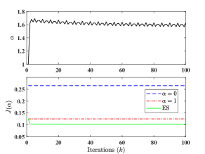
Finally, we provide a simulation to illustrate the performance optimization idea with a factor α\alpha discussed in Section V. We will use the ES algorithm in the iteration domain from [35] to find an optimal α\alpha. The quadratic cost J(α)J(\alpha) in (134) is used with T=100sT=100s. The disturbance signal w1=sin(1.5πt)w_{1}=\sin(1.5\pi t) is considered in the α\alpha tuning process and the result is shown in Fig. 17. It is seen that the parameter α\alpha converges to a small neighborhood of α=1.60\alpha^{*}=1.60 which yields a lower cost J(α=α)=0.1035J(\alpha=\alpha^{*})=0.1035 compared with the cases when α=0\alpha=0 (J(α=0)=0.2654J(\alpha=0)=0.2654, LQT performance) and α=1\alpha=1 (J(α=1)=0.1256J(\alpha=1)=0.1256, MOCC performance).

Refer to caption
Figure 17: α\alpha tuning in the presence of w1.w_{1}.

VII Conclusion

A multi-objective complementary control (MOCC) framework that can assemble two independently designed controllers in a complementary way instead of a trade-off is proposed. A state-space realization for the Youla-type operator 𝑸{\bm{Q}} is provided to manage the two controllers. In particular, an MO complementary tracking control is applied to demonstrate the advantages of MOCC. Rigorous performance analysis shows that the tracking performance and robustness can be addressed separately, especially when the disturbance signal is independent of the reference signal. Simulation results validate the advantages of MOCC, especially, when the disturbance signal is completely unknown. Furthermore, it is shown that this framework can be potentially extended to improve the total performance through a data-driven approach with an extra gain factor to 𝑸\bm{Q}.

References

  • [1] P. P. Khargonekar and M. A. Rotea, “Multiple objective optimal control of linear systems: The quadratic norm case,” IEEE Transactions on Automatic Control, vol. 36, no. 1, pp. 14–24, 1991.
  • [2] C. Scherer, P. Gahinet, and M. Chilali, “Multiobjective output-feedback control via LMI optimization,” IEEE Transactions on Automatic Control, vol. 42, no. 7, pp. 896–911, 1997.
  • [3] N. Elia and M. A. Dahleh, “Controller design with multiple objectives,” IEEE Transactions on Automatic Control, vol. 42, no. 5, pp. 596–613, 1997.
  • [4] X. Chen and K. Zhou, “Multiobjective H2{H_{2}}/H{H_{\infty}} control design,” SIAM Journal on Control and Optimization, vol. 40, no. 2, pp. 628–660, 2001.
  • [5] C. Lin and B.-S. Chen, “Achieving pareto optimal power tracking control for interference limited wireless systems via multi-objective H2/H{H}_{2}/{H}_{\infty} optimization,” IEEE Transactions on Wireless Communications, vol. 12, no. 12, pp. 6154–6165, 2013.
  • [6] L. Menini, C. Possieri, and A. Tornambè, “Algebraic methods for multiobjective optimal design of control feedbacks for linear systems,” IEEE Transactions on Automatic Control, vol. 63, no. 12, pp. 4188–4203, 2018.
  • [7] D. V. Balandin and M. M. Kogan, “Multi-objective generalized H2{H}_{2} control,” Automatica, vol. 99, pp. 317–322, 2019.
  • [8] P. Bhowmick and S. Patra, “Solution to negative-imaginary control problem for uncertain LTI systems with multi-objective performance,” Automatica, vol. 112, p. Art. no. 108735, 2020.
  • [9] H.-G. Han, C. Chen, H.-Y. Sun, and J.-F. Qiao, “Multiobjective integrated optimal control for nonlinear systems,” IEEE Transactions on Cybernetics, early access, 2022, doi: 10.1109/TCYB.2022.3204030.
  • [10] D. Bernstein and W. Haddad, “LQG control with an H{H}_{\infty} performance bound: A Riccati equation approach,” IEEE Transactions on Automatic Control, vol. 34, no. 3, pp. 293–305, 1989.
  • [11] P. P. Khargonekar and M. A. Rotea, “Mixed H2/H{H}_{2}/{H}_{\infty} control: A convex optimization approach,” IEEE Transactions on Automatic Control, vol. 36, no. 7, pp. 824–837, 1991.
  • [12] D. J. Limebeer, B. D. Anderson, and B. Hendel, “A Nash game approach to mixed H2/H{H}_{2}/{H}_{\infty} control,” IEEE Transactions on Automatic Control, vol. 39, no. 1, pp. 69–82, 1994.
  • [13] K. Zhou, K. Glover, B. Bodenheimer, and J. Doyle, “Mixed H2{H}_{2} and H{H}_{\infty} performance objectives I: Robust performance analysis,” IEEE Transactions on Automatic Control, vol. 39, no. 8, pp. 1564–1574, 1994.
  • [14] J. Doyle, K. Zhou, K. Glover, and B. Bodenheimer, “Mixed H2{H}_{2} and H{H}_{\infty} performance objectives II: Optimal control,” IEEE Transactions on Automatic Control, vol. 39, no. 8, pp. 1575–1587, 1994.
  • [15] H. A. Hindi, B. Hassibi, and S. P. Boyd, “Multiobjective H2/H{H}_{2}/{H}_{\infty}-optimal control via finite dimensional qq-parametrization and linear matrix inequalities,” in Proceedings of the 1998 American Control Conference (ACC), 1998, pp. 3244–3249.
  • [16] D. Youla and J. Bongiorno, “A feedback theory of two-degree-of-freedom optimal Wiener-Hopf design,” IEEE Transactions on Automatic Control, vol. 30, no. 7, pp. 652–665, 1985.
  • [17] J. Moore, L. Xia, and K. Glover, “On improving control-loop robustness of model-matching controllers,” Systems & Control Letters, vol. 7, no. 2, pp. 83–87, 1986.
  • [18] C. Wen, J. Lu, and W. Su, “Bi-objective control design for vehicle-mounted mobile antenna servo systems,” IET Control Theory & Applications, vol. 16, no. 2, pp. 256–272, 2022.
  • [19] K. Zhou and Z. Ren, “A new controller architecture for high performance, robust, and fault-tolerant control,” IEEE Transactions on Automatic Control, vol. 46, no. 10, pp. 1613–1618, 2001.
  • [20] J. Chen, S. Hara, and G. Chen, “Best tracking and regulation performance under control energy constraint,” IEEE Transactions on Automatic Control, vol. 48, no. 8, pp. 1320–1336, 2003.
  • [21] J. Chen, L. Qiu, and O. Toker, “Limitations on maximal tracking accuracy,” IEEE Transactions on Automatic Control, vol. 45, no. 2, pp. 326–331, 2000.
  • [22] M. Vidyasagar, Control Systems Synthesis: A Factorization Approach, Part I.   Switzerland: Springer, 2022.
  • [23] B. D. Anderson, “From Youla–Kucera to identification, adaptive and nonlinear control,” Automatica, vol. 34, no. 12, pp. 1485–1506, 1998.
  • [24] X. Chen, K. Zhou, and Y. Tan, “Revisit of LQG control–A new paradigm with recovered robustness,” in Porceedings of the IEEE 58th Conference on Decision and Control (CDC), 2019, pp. 5819–5825.
  • [25] K. Zhou, J. Doyle, and K. Glover, Robust and optimal control.   Englewood Cliffs, NJ, USA: Prentice-Hall, 1996.
  • [26] A. Q. Keemink, H. van der Kooij, and A. H. Stienen, “Admittance control for physical human–robot interaction,” Int. J. Robot. Res., vol. 37, no. 11, pp. 1421–1444, 2018.
  • [27] P. Mäkilä, J. Partington, and T. Norlander, “Bounded power signal spaces for robust control and modeling,” SIAM Journal on Control and Optimization, vol. 37, no. 1, pp. 92–117, 1998.
  • [28] Y. Wan, W. Dong, H. Wu, and H. Ye, “Integrated fault detection system design for linear discrete time-varying systems with bounded power disturbances,” International Journal of Robust and Nonlinear Control, vol. 23, no. 16, pp. 1781–1802, 2013.
  • [29] A. V. Oppenheim, A. S. Willsky, S. H. Nawab, and J.-J. Ding, Signals and systems, 2nd ed.   Upper Saddle River, NJ, USA: Prentice-Hall, 1997.
  • [30] W. A. Gardner and E. A. Robinson, Statistical spectral analysis: A nonprobabilistic theory.   Englewood Cliffs, NJ, USA: Prentice-Hall, 1988.
  • [31] F. J. Vargas, E. I. Silva, and J. Chen, “Stabilization of two-input two-output systems over SNR-constrained channels,” Automatica, vol. 49, no. 10, pp. 3133–3140, 2013.
  • [32] K. Glover and J. C. Doyle, “State-space formulae for all stabilizing controllers that satisfy an H{H}_{\infty}-norm bound and relations to relations to risk sensitivity,” Systems & Control Letters, vol. 11, no. 3, pp. 167–172, 1988.
  • [33] B. D. Anderson and J. B. Moore, Optimal control: Linear quadratic methods.   Englewood Cliffs, NJ, USA: Prentice-Hall, 1989.
  • [34] U. Shaked and C. E. de Souza, “Continuous-time tracking problems in an H{H_{\infty}} setting: A game theory approach,” IEEE Transactions on Automatic Control, vol. 40, no. 5, pp. 841–852, 1995.
  • [35] N. J. Killingsworth and M. Krstic, “PID tuning using extremum seeking: Online, model-free performance optimization,” IEEE Control Systems Magazine, vol. 26, no. 1, pp. 70–79, 2006.
  • [36] D. A. Bristow, M. Tharayil, and A. G. Alleyne, “A survey of iterative learning control,” IEEE Control Systems Magazine, vol. 26, no. 3, pp. 96–114, 2006.
  • [37] S. Z. Khong, D. Nešić, and M. Krstić, “Iterative learning control based on extremum seeking,” Automatica, vol. 66, pp. 238–245, 2016.
  • [38] K. B. Ariyur and M. Krstic, Real-time optimization by extremum-seeking control.   NJ: John Wiley & Sons, 2003.
  • [39] Y. Tan, D. Nešić, and I. Mareels, “On non-local stability properties of extremum seeking control,” Automatica, vol. 42, no. 6, pp. 889–903, 2006.
  • [40] J. Xu, Y. Tan, and X. Chen, “Robust tracking control for nonlinear systems: Performance optimization via extremum seeking,” in Proceedings of the 2023 American Control Conference (ACC), 2023, pp. 1523–1528.
  • [41] W.-H. Chen, J. Yang, L. Guo, and S. Li, “Disturbance-observer-based control and related methods—An overview,” IEEE Transactions on Industrial Electronics, vol. 63, no. 2, pp. 1083–1095, 2016.
  • [42] J. Yang, A. Zolotas, W.-H. Chen, K. Michail, and S. Li, “Robust control of nonlinear MAGLEV suspension system with mismatched uncertainties via DOBC approach,” ISA Transactions, vol. 50, no. 3, pp. 389–396, 2011.